Deep ice layer formation in an alpine snowpack: monitoring and modeling

Ice layers may form deep in the snowpack due to preferential water flow, with impacts on the snowpack mechanical, hydrological and thermodynamical properties. This detailed study at a high-altitude alpine site aims to monitor their formation and evolution thanks to the combined use of a comprehensive observation dataset at a daily frequency and state-of-the-art snow-cover modeling with improved ice formation representation. In particular, daily SnowMicroPen penetration resistance profiles enabled us to better identify ice layer temporal and spatial heterogeneity when associated with traditional snowpack profiles and measurements, while upward-looking ground penetrating radar measurements enabled us to detect the water front and better describe the snowpack wetting when associated with lysimeter runoff measurements. A new ice reservoir was implemented in the one-dimensional SNOWPACK model, which enabled us to successfully represent the formation of some ice layers when using Richards equation and preferential flow domain parameterization during winter 2017. The simulation of unobserved melt-freeze crusts was also reduced. These improved results were confirmed over 17 winters. Detailed snowpack simulations with snow microstructure representation associated with a high-resolution comprehensive observation dataset were shown to be relevant for studying and modeling such complex phenomena despite limitations inherent to one-dimensional modeling.

1 Introduction

The presence of ice layers in a snowpack may impact its mechanical, hydrological and thermodynamical properties. Monitoring the formation and evolution of ice layers is thus crucial in many research fields. Because of their low permeability (Albert and Perron, 2000), ice layers may increase the liquid water storage of the snowpack, which can substantially affect the snowpack runoff (Singh et al., 1999). In contrast, near-surface ice layers in Greenland were shown to prevent access to deeper firn layers, thus reducing meltwater storage in the firn and enhancing ice sheet mass loss (Machguth et al., 2016). The stability of a mountainous snowpack may also be affected, with a possible increased faceting of the microstructure close to ice or crusts (Jamieson, 2006; Hammonds et al., 2015; Hammonds and Baker, 2016). Moreover, retrieval algorithms for the water equivalent of snow cover and snow depth from passive microwave emissions are sensitive to the presence of ice layers (Rees et al., 2010; Roy et al., 2016). Better knowledge about their formation could help the assimilation of such data in detailed snow-cover models (Larue et al., 2018).

Ice forms in the snowpack can have different origins (Fierz et al., 2009). They can form either at the surface because of freezing rain (Quéno et al., 2018) or a firnspiegel formation process due to radiative cooling (Ozeki and Akitaya, 1998) or within the snowpack through the percolation of rain or meltwater reaching subfreezing snow (Pfeffer and Humphrey, 1998). The present study focuses on the latter case. As opposed to matrix water flow leading to a homogeneous progression of the wetting front, preferential water flow occurs through flow fingering (e.g., Schneebeli, 1995) transporting liquid water to deeper regions of the snowpack where the cold content is sufficient to refreeze it (e.g., Marsh, 2006). Preferential flow occurs in the snowpack due to its microstructural heterogeneity (density, grain size and shape) at layer transitions (Katsushima et al., 2013), which may trigger flow fingering or form hydraulic barriers (i.e., capillary or permeability barriers) where water ponds and may subsequently refreeze. Hydraulic barriers may also divert water flow and lead to lateral flow along slopes (Eiriksson et al., 2013; Webb et al., 2018a). Knowledge about water percolation in snow, and particularly preferential flow, has recently greatly expanded in terms of process understanding and numerical simulation. Using dye tracer and liquid water content (LWC) measurements, Avanzi et al. (2016) observed preferential flow and water ponding at capillary barriers for various layer transition characteristics and water input. X-ray microtomography was also used to observe wet-snow metamorphism under preferential flow (Avanzi et al., 2017). Magnetic resonance imaging observations of finger flow and lateral flow emphasized that even small differences in snow properties may form capillary barriers in dry snow (Katsushima et al., 2018, 2020). At larger scales, the effect of preferential flow on the snowpack runoff was assessed through measurements of the heterogeneity of water discharge (Yamaguchi et al., 2018; Webb et al., 2018b) or under rain-on-snow conditions (Würzer et al., 2017; Juras et al., 2017). The new insights from measurement campaigns enabled the development of multidimensional models that account for preferential flow in the snowpack (Hirashima et al., 2014, 2017, 2019; Leroux and Pomeroy, 2017, 2019). They also enabled progress in the representation of water transport in one-dimensional (1-D) models. The Richards equation was implemented in detailed snow-cover models like SNOWPACK (Wever et al., 2014) and Crocus (D'Amboise et al., 2017) as an improvement over the more simplistic bucket parameterization, enabling a more realistic representation of water transport in snow with respect to snow microstructure. Based on recent studies relating preferential flow to snow properties (Katsushima et al., 2013; Hirashima et al., 2014; Yamaguchi et al., 2012) with analogies to preferential flow in soils (DiCarlo, 2007, 2013), Wever et al. (2016) developed an original 1-D parameterization of preferential flow in SNOWPACK through a dual-domain implementation separating matrix flow and preferential flow, both of which are solved with the Richards equation.

The representation of ice layer formation in snow-cover models remains very challenging because it depends on an accurate description of the snow microstructure and water transport. Currently, most snow-cover models do not take into account the processes of ice layer formation. Quéno et al. (2018) recently modeled ice formation on the snowpack surface due to freezing precipitation in the detailed snow-cover model Crocus. Wever et al. (2016) included for the first time in a detailed snow-cover model the process of deep ice layer formation due to preferential water flow. Using the dual-domain implementation for water percolation in a subfreezing snowpack, they investigated ice layer formation at an alpine site, comparing manual snow profiles recorded every 2 weeks over 16 winter seasons with SNOWPACK simulations. Nevertheless, many research gaps remain open about deep ice layer formation in a snowpack. In particular, the present study aims at answering the following questions.

• Can daily SnowMicroPen (SMP) measurements improve the monitoring of ice layers in natural snowpacks over traditional snowpack profiling?

• How well can 1-D snow-cover models represent a multidimensional process like ice formation due to preferential flow?

• Can spatially discontinuous ice lenses be parameterized in a 1-D snow-cover model?

• Can we provide useful information on ice layer origin and evolution in alpine snowpacks for various applications based on observations and simulations?

To address these research questions, we bring several novelties in a detailed study pushing forward the investigation of Wever et al. (2016). First, a comprehensive observation dataset was gathered at the same research site in order to better determine the evolution of the snowpack and identify the formation of deep ice layers in natural conditions at a high-altitude alpine site. The originality of this dataset comes from the opportunity to monitor ice formation in natural alpine conditions during a whole winter season at daily resolution even though the present study does not include detailed observations of preferential water flow paths. This dataset is then used for a detailed assessment of the preferential flow representation in SNOWPACK, bringing complementary insights to Wever et al. (2016) and Würzer et al. (2017). As a result, we introduce a new parameterization to improve the simulation of discontinuous deep ice formation in the SNOWPACK model.

The paper is organized as follows. Section 2 describes the study site, the observation dataset, the snowpack simulation configuration and new methods. Section 3 details the results with insights on water percolation and ice layer formation from both the observation dataset and the simulations. Their benefits and limitations are discussed in Sect. 4.

2 Data and methods

2.1 Observation dataset

The site of study is the Weissfluhjoch (WFJ) measurement site, a research field dedicated to snowpack investigations which is located at an elevation of 2536 m above sea level by Davos in the eastern Swiss Alps (Marty and Meister, 2012). For comparison to simulations, we use a comprehensive observation dataset collected during winter 2017. Figure 1 indicates the location of the measurements in the research field. Traditional snowpack profiles were performed during the entire season every week (or every 2 weeks at the beginning and the end of the season) along three corridors, moving continuously along each corridor and turning into the next one once the end of the previous one had been reached. These profiles were carried out following the recommendations of Fierz et al. (2009), and they gather observations of the grain shape, grain size, layer thickness, hand hardness index and wetness through visual and manual assessments, as well as measurements of snow depth (HS), water equivalent of snow cover (SWE), snow density, snow temperature, snow hardness (Swiss ramsonde) and liquid water content with a Denoth device (Denoth, 1989). Continuous melt-freeze crusts (MFcrs) and ice layers (IFils) were identified in the snow profile, while ice lenses were most often noted additionally. There was no measurement of ice layer density as such measurements in natural conditions remain very challenging (e.g., Watts et al., 2016). Snowpack runoff measurements were provided by a 5 m² lysimeter at 10 min temporal resolution (Wever et al., 2014). Finally, thermistors at a fixed vertical interval of 20 cm provided half-hourly snow temperature profiles of the snowpack (Fierz, 2011).

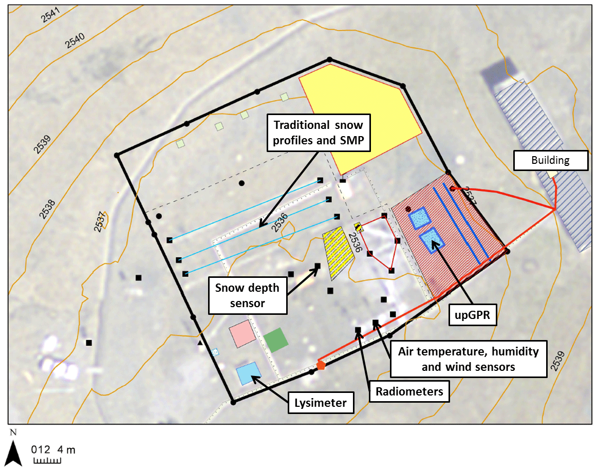
Figure 1 Overview of the WFJ research field with contour lines in orange and labels indicating the location of the measurements used in this study.

An upward-looking ground penetrating radar (upGPR) was also installed at the site (Schmid et al., 2014). The dual frequency GPR from IDS (Ingegneria Dei Sistemi, Italy) conducted measurements every 30 min and with two different frequencies, 600 MHz and 1.6 GHz. Every measurement contained 1800 traces with 1024 samples. In order to remove system ringing, a hoisting device was installed by Schmid et al. (2014) to move the GPR antennas vertically during a measurement cycle. When transmitting electromagnetic waves into snow, discontinuities result in reflections, refractions and diffractions. The amount of energy reflected at the discontinuity is proportional to the relative change across the discontinuity (Reynolds, 2011). The percolated water changes the internal properties of the snow. The boundary between wet and dry snow (called water front hereafter) appears as a distinct reflector and can then be determined by semiautomatic picking similar to the algorithm developed by Schmid et al. (2014) for snow surface picking. The picked two-way travel times of the water front are multiplied by the wave propagation velocity of 0.23 m ns⁻¹, which is a typical value for snow (Sand and Bruland, 1998; Schmid et al., 2014). During winter 2017, the water front could be derived until a technical malfunction on 9 April prevented further analysis. Due to the 45^∘ angle of beam spread of the upGPR, the footprint in the snowpack where the water front is derived enables us to identify a homogeneous state but not local flow fingers.

In addition, daily measurements of the penetration resistance were performed with a SnowMicroPen (Schneebeli et al., 1999) in the context of the RHOSSA field campaign (Calonne et al., 2020) launched in winter 2016. The SMP has a tip surface of 19.6 mm². Every day during the winter season, five to seven SMP measurements were performed moving forward by steps of about 40 cm along the corridors, with a 15 cm spacing perpendicular to the direction of the corridor providing indications of the local spatial heterogeneity of potential ice forms. A limited number of gaps in the daily measurements have to be noted, in particular from 25 to 27 March and 7 to 8 April in the wetting period.

For longer-term observations of ice layers, we gathered traditional snowpack profiles performed every 2 weeks during the winter seasons 1999/2000 to 2015/2016.

The comprehensive observation dataset of winter 2017 at WFJ is publicly available (see Code and Data Availability section).

2.2 Snowpack simulations

2.2.1 Simulation configuration

SNOWPACK simulations were performed for the WFJ study site in winter 2017. They were initialized with a traditional profile recorded on 3 January 2017 to provide a realistic base of the snowpack with a snow depth of 47 cm. The initialization date were chosen to be early enough to assess the model's ability to simulate the microstructure evolution, as well as water percolation, but to avoid early season modeling errors, for example, the formation of unobserved basal melt-freeze layers. The simulations were driven by optimal in situ meteorological measurements (Fig. 1) of air temperature and humidity (ventilated sensors), near-surface wind, and solar and longwave irradiance (WSL Institute for Snow and Avalanche Research SLF, 2015; Wever et al., 2015). The snowfall input is driven by measured snow depth increments (Wever et al., 2015) enabling direct comparisons to the measurements and outcomes of Wever et al. (2016). In addition, for air temperatures above 1.2 ^∘C, undercatch-corrected precipitation gauge measurements are considered to be rain.

Three water transport schemes implemented in SNOWPACK were evaluated. First, the bucket approach (BA) is a common method used in snow-cover models (e.g., Bartelt and Lehning, 2002; Vionnet et al., 2012), which assumes that water is transported to the next downward layer when the liquid water content exceeds the water holding capacity of a given layer (depending on the ice volumetric content of snow; Coléou and Lesaffre, 1998). Second, the Richards equation (RE) was implemented in SNOWPACK by Wever et al. (2014) to account for capillary effects. These effects are modeled taking into account the water retention curve (van Genuchten, 1980) and the hydraulic conductivity of snow (Mualem, 1976; van Genuchten, 1980; Calonne et al., 2012). Third, a dual-domain approach parameterizing preferential flow (PF) and using the Richards equation (RE/PF) was recently developed. Water exchanges between the matrix domain and the preferential flow domain are determined according to the water entry pressure head in the matrix layers and the saturation in the preferential flow domain; this implementation is described in details in Wever et al. (2016). The two tuning parameters of this scheme were chosen here according to Wever et al. (2016): the threshold in saturation of the preferential flow domain, Θ_th=0.08, and the parameter related to the number of flow paths per square meter, N=0. In particular, N=0 implies no refreezing of the preferential flow water (Wever et al., 2016). Similar to Wever et al. (2016), SNOWPACK simulations were carried out at high vertical resolution with a layer-merging threshold of 0.25 cm and new snow layer initialization of 0.5 cm. A high resolution is necessary to permit the formation of very thin high density layers.

2.2.2 Implementation of ice reservoir

A new parameterization of ice layer formation due to preferential flow was implemented as a complement to the RE/PF scheme. It is summarized in Fig. 2. In the RE/PF scheme, when the saturation in the preferential flow domain exceeds the threshold Θ_th, water flows back to the matrix domain. First, a volume of water corresponding to the available freezing capacity is instantly frozen and added uniformly to the ice content of the matrix domain. Ice lenses, in contrast, may only form locally at the base of the flow fingers. If the threshold is still exceeded, then saturations in both domains are equalized (Wever et al., 2016).

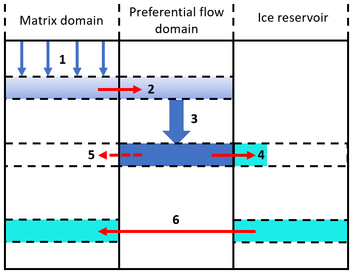
Figure 2 Scheme of the ice reservoir parameterization in SNOWPACK. Blue represents liquid water, cyan represents ice, and red arrows represent water or ice transfers to another domain. Steps 1 to 6 are described in the text.

To better reproduce the formation of continuous ice layers from discontinuous and growing ice lenses, we developed an ice reservoir parameterization. The water, which is normally transferred from the preferential flow domain to the matrix domain that freezes instantly, is stored in an ice reservoir (step 4 in Fig. 2) instead of being added to the ice volumetric content of the matrix. The ice reservoir is representative of the volumetric content of ice lenses (i.e., spatially discontinuous ice) in a given layer. The transferred water that does not freeze goes in the matrix domain, i.e., is spread homogeneously (step 5 in Fig. 2).

Furthermore, the saturation threshold in the PF domain (Wever et al., 2016) was chosen as a simple solution to the inability of the Richards equation to model the saturation overshoot present in the tip of flow fingers (DiCarlo, 2007). This simple parameterization can lead to inconsistencies due to the vertical discretization of the simulated snowpack. After water has been transferred to the matrix at the layer corresponding to the finger tip (i.e., where the saturation threshold was exceeded), the highest saturation is then more likely reached at the layer above where no water transfer occurred because water percolation from this layer to the finger tip layer only occurs at the next time step. Because of that, the water transfer from the PF domain to the matrix domain may spread over too many layers instead of being concentrated in the lowest layer (i.e., the tip of the flow finger). To overcome this issue, the ice reservoir was cumulated in the lowest layer. When the ice volumetric content of the cumulated ice reservoir plus the ice volumetric content and water volumetric content of the associated matrix layer exceed the corresponding ice density threshold of 700 kg m⁻³ in SNOWPACK, there is enough ice to consider it horizontally homogeneous; the ice content of the cumulated ice reservoir is then transferred to the associated matrix layer (step 6 in Fig. 2). As long as it is kept in the ice reservoir, the forming ice has no effect on the water transport in the matrix domain that still follows the RE/PF scheme (Wever et al., 2014, 2016). Furthermore, we neglect any impact the ice reservoir, which is interpreted as ice lenses, may have on hydraulic properties (e.g., local hydraulic barrier effect). Simulations with the ice reservoir parameterization are called RE/PF/IceR hereafter.

The implementation of the ice reservoir parameterization in the SNOWPACK source code is publicly available (see Code and Data Availability section).

3 Results

3.1 Insights from the observation dataset

3.1.1 Overview of the winter season

At WFJ, winter 2016/2017 started with a shallow snowpack of approximately 30 cm at the beginning of November, followed by a extended period of calm weather, forming a base layer made of depth hoar crystals (Richter et al., 2019). This layer was covered by new snow at the end of December, and several small snow storms led to a maximum snow depth of 205 cm on 10 March, i.e., slightly lower than the average maximum snow depth. The snowpack had entirely melted on 14 June. Overall, this winter was characterized by a lower snow depth than the long-term averages in the region.

Figure 3 represents the evolution of grain types within the snowpack as observed in traditional snow profiles. Two layers of particular interest are tracked during the whole winter. Layer 1 corresponds to surface hoar formed at the end of January. This layer is continuously identified as buried surface hoar (as primary or secondary grain) until the end of March with a grain size substantially larger than the layer above (consisting of rounded grains or faceted crystals), thus constituting a capillary barrier with a classical fine-over-coarse structure (e.g., Avanzi et al., 2016). Ice is observed above this barrier from 28 March either as a homogeneous layer or as ice lenses mixed with melt forms (red in Fig. 3). Thicknesses between 0.5 and 1 cm were reported. The presence of nearby slopes (NNW of the snow profile corridors in Fig. 1) may suggest a water input through lateral flow along the capillary barrier. Simulations (not taking into account lateral flow) may provide complementary insights to determine whether vertical preferential flow was sufficient to form an ice layer. Layer 2 corresponds to surface hoar appearing in mid-February and forming a capillary barrier once buried. An ice layer is observed at that level in most profiles after 28 March.

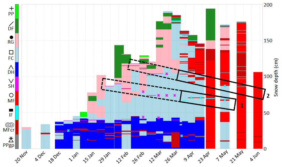
Figure 3 Visual observations of grain shapes at WFJ during winter 2017. Colors, symbols and codes are defined following the grain shape classification of Fierz et al. (2009), fuchsia crosses represent surface hoar as secondary grain shape, and cyan crosses represent ice lenses. Rectangles highlight layers 1 and 2 with dashed lines before ice formation and solid lines afterwards.

3.1.2 Water percolation and snowpack runoff

Figure 4 represents lysimeter measurements of the snowpack runoff, together with the height of the water front estimated from the upGPR measurements, from 1 March to 15 April, i.e., the transition period from dry to isothermal snowpack. Shown underneath are the snow temperature measurements in the lowest meter of the snowpack at fixed intervals of 20 cm. The height of the water front could only be derived until 8 April due to technical issues. Before 30 March (first dashed line), no snowpack runoff was observed, the water front was always higher than 1 m, and temperatures in the lowest first meter of the snowpack were all below 0 ^∘C. Between 30 March and 9 April (second dashed line), the water front remained high (mostly higher than 1 m), and a small amount of snowpack runoff was observed (less than 3 $\mathrm{kg}{\mathrm{m}}^{-\mathrm{2}}{\mathrm{d}}^{-\mathrm{1}}$). Snow temperatures gradually increased to reach 0 ^∘C by the end of the period in the lowest meter of the snowpack. From 9 April, all temperatures in the lowest meter reached 0 ^∘C, and snowpack runoff increased. Although after 9 April no more water front estimates were available from the upGPR data, it reached the lowest value (85 cm) on 8 April. The snowpack runoff is yet low compared to the more significant runoff starting in mid-May, as shown in Fig. 5; the first 20 kg m⁻² of total snowpack runoff was reached on 10 April, while the first day with a daily snowpack runoff higher than 10 $\mathrm{kg}{\mathrm{m}}^{-\mathrm{2}}{\mathrm{d}}^{-\mathrm{1}}$ was 13 May.

Figure 4 (a) Evolution of the snow depth (black line), height of the water front (blue line) and daily snowpack runoff (blue bars) from 1 March to 15 April 2017 at WFJ. (b) Measured snow temperatures at different heights above the ground are from the same period and same location. Dashed lines indicate 30 March and 9 April.

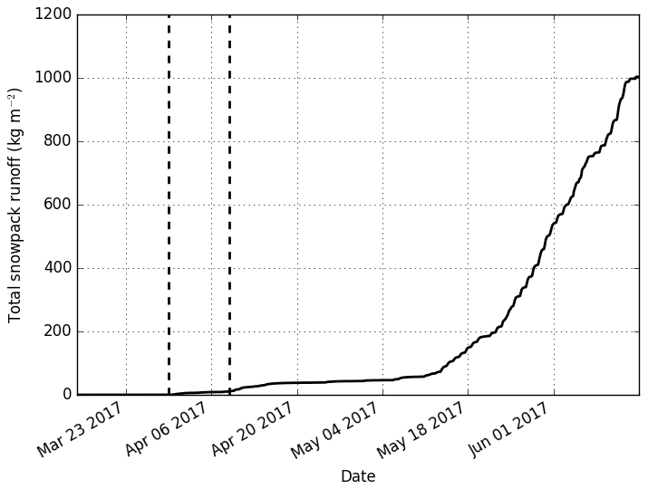
Figure 5 Total snowpack runoff from 15 March to 15 June 2017 at WFJ. Dashed lines indicate 30 March and 9 April.

These measurements give insights in the timing of water percolation in the snowpack. Before 9 April, the bottom of the snowpack was cold and dry, while the water front was still mostly above 100 cm. The low snowpack runoff values were thus likely due to preferential flow paths reaching the ground. After 9 April, the lowest meter of the snowpack reached an isothermal state at 0 ^∘C, and snowpack runoff increased markedly.

3.1.3 Capillary barriers and ice layers

To study the formation of ice through preferential flow in subfreezing snow, we focus on the lowest meter of the snowpack. In this part, the manual snow profiles enable us to identify three main capillary barriers (Fig. 3): the two layers of buried surface hoar where ice forms at the end of March (defined as layers 1 and 2 previously) and the top of the depth hoar base layer, where higher water content is observed in April and May. Layers 1 and 2 are marked by grain size heterogeneity with the overlying layers: on 28 February, 1 mm over 2.5 mm for layer 1 and 0.5 mm over 2 mm for layer 2.

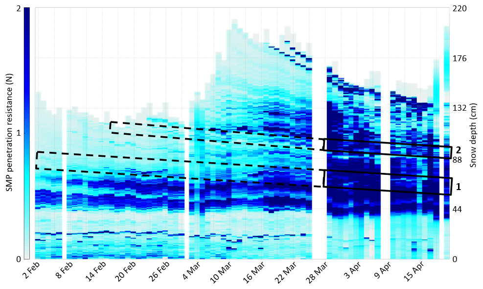
Figure 6 Daily SMP measurements of penetration resistance (mm, averaged values) at WFJ from 1 February to 19 April with one representative profile per day. Values higher than 2 N are shown with the same color. Rectangles highlight the approximate location of layers 1 and 2 with dashed lines before ice formation and solid lines afterwards.

Daily SMP measurements enable us to more clearly identify the temporal and spatial variability of ice formation. Figure 6 represents the evolution of penetration resistance from 1 February to 19 April with a scale from 0 to 2 N to highlight variations in dry snow. The deep MFcr is visible in the middle of a low-resistance depth hoar layer at approximately 20 cm. In February and March, the highest values in the middle of the snowpack correspond to dense layers of faceted crystals (Fig. 3). In March, the buried surface hoar of layer 1 is marked by a lower penetration resistance than the surrounding faceted crystals. Layer 2 exhibits less heterogeneity with surrounding layers. Overall, the penetration resistance increases substantially from the end of March onwards with the progressive wetting, particularly at the top of the snowpack where many melt-freeze crusts form. Figure 7a represents penetration resistances higher than thresholds of 5 and 10 N below 100 cm and includes all daily SMP measurements. These values were chosen after a comparison of matching traditional and SMP profiles to better highlight crusts and ice forms. Except the deep MFcr mostly visible until the end of March, two high resistance layers can be identified from 29 March; they match the visual identification of ice layers 1 and 2 (Fig. 7b). They can be tracked until mid-April but are not present in all SMP profiles.

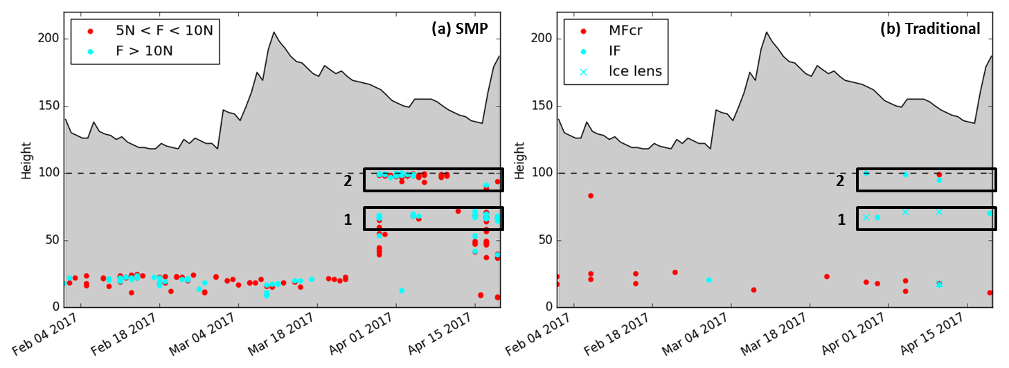
Figure 7 (a) Height of SMP penetration resistances between 5 and 10 N (red) and higher than 10 N (cyan) below 1 m from 1 February to 19 April at WFJ. (b) Visual observations of melt-freeze crusts (MFcr), ice layers (IFil) and ice lenses at the same period and location. Daily manual measurements of snow depth in solid black lines. Rectangles highlight layers 1 and 2.

The penetration resistance measured at these two layers was tracked in the SMP profiles. To identify these layers, all SMP profiles were superimposed on the traditional profile observed at the closest date. Penetration resistances were associated with observed snow layers given their grain type and hand hardness index. To identify consistent patterns, the SMP profiles of a given day were also compared among each other and with those of the previous and next days. The value of SMP penetration resistance in these layers was then visually picked. Figure 8 shows an example of this procedure for the two SMP profiles of 4 April 2017.

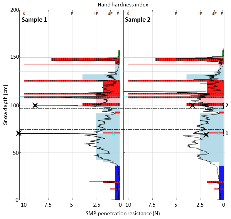
Figure 8 Two samples of SMP profiles of 4 April 2017 (black line) superimposed on the traditional snow profile of the same date. Colors referring to the grain shape and hand hardness index are defined accordingly to the classification of Fierz et al. (2009). Cyan crosses indicate ice lenses. Dashed rectangles highlight layers 1 and 2. Black crosses indicate the penetration resistance picked for each layer.

The evolution of the penetration resistance of the two tracked layers is plotted in Fig. 9 from 14 March to 19 April. For layer 1, the penetration resistance remains very low (less than 1 N) until 24 March. It corresponds to the observed layer of buried surface hoar. On 29 March, all seven SMP measurements show penetration resistances higher than 10 N, indicating the continuous presence of ice. Afterwards, values alternate between low resistance (less than 5 N) and very high resistance (more than 10 N), as visible in Fig. 8 on 4 April. This is consistent with the visual observations reporting a layer in which pure ice and melt forms are both observed. These observations suggest that water ponding at the capillary barrier did not freeze everywhere on the study plot where we performed these measurements. For layer 2, very low penetration resistances are also measured until 24 March, corresponding to the observed buried surface hoar. After 29 March, values increase (mostly higher than 5 N, often more than 10 N), indicating the formation of ice. After 9 April, no more high resistances are measured but rather low resistances corresponding to a wet layer of melt forms. The evolution of penetration resistances for layer 2 show more temporal consistency than layer 1, suggesting that the ice layer disappears totally after 9 April.

Figure 9 Evolution of the penetration resistance of (a) layer 1 and (b) layer 2, manually tracked in the SMP profiles, from 14 March to 19 April. Thresholds of 5 and 10 N are indicated in red and cyan, respectively, accordingly to Fig. 7.

3.2 Assessment of snowpack simulations

3.2.1 Assessment with different water transport schemes

Simulations of winter 2017 were first performed with the three water transport schemes existing in SNOWPACK (BA, RE and RE/PF). For the RE/PF simulation, Fig. 10 shows the grain shape and liquid water content in the PF domain for the month of February. Buried surface hoar of layer 1 (represented in fuchsia and at approximately 80 cm) is well simulated at the beginning of February. The capillary barrier of layer 2 is also well initiated in mid-February on the surface. However, a thick melt-freeze crust forms at layer 1 on 10 February (represented in hatched red, Fig. 10a). It is associated with some melting close to the surface leading to preferential water flow refreezing at the capillary barrier of layer 1 (Fig. 10b). The water transferred for refreezing in the matrix domain is spread homogeneously, which forms a crust with a density of approximately 320 kg m⁻³. The transfer spreads vertically due to the issues mentioned in Sect. 2.2.2. This thick melt-freeze crust was not observed in the manual profiles nor the SMP measurements. Other melt-freeze crusts form close to the surface from mid-February. They were observed (Fig. 3) but were thinner than the simulated ones. A little surface melting is simulated on 1 February and leads to preferential flow (Fig. 10). Contrary to later simulated melting in mid-February, it was not observed; the measured snow surface temperature remained slightly under melting point. This simulation error is likely due to excessive surface turbulent flux inputs. New simulations were run without this melt water input with no effect on the later snowpack structure due to the limited melting amount.

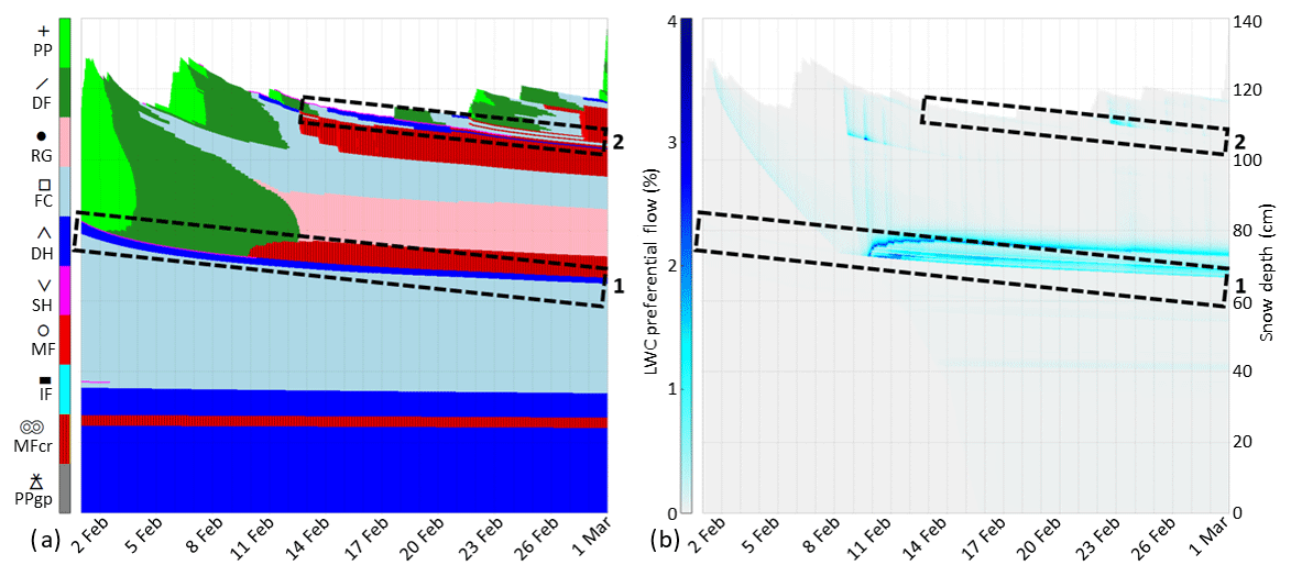
Figure 10 SNOWPACK simulation RE/PF in February 2017 at WFJ: (a) grain shape according to the classification of Fierz et al. (2009), and (b) liquid water content in the PF domain. Rectangles highlight layers 1 and 2.

Figure 11 shows the grain shape and the liquid water content in the matrix domain from 15 March to 15 April, i.e., the period of transition from dry to ripe snowpack when ice layers formed (Sect. 3.1). No ice layer forms except at the snowpack basis, which is probably due to a boundary effect at the interface between snow and soil. The thick melt-freeze crust is still present at layer 1, and thus no ice layer forms (Fig. 11a). However, a higher water retention is simulated (Fig. 11b). Due to the excessive formation of melt-freeze crusts, the simulated snow microstructure at layer 2 does not reproduce the observed snow microstructure and the capillary barrier, and thus no ice layer forms. Matrix flow reaches the ground, and the snowpack is entirely isothermal on 31 March (Fig. 11b), i.e., 9 d before the observations (Sect. 3.1.2). On 31 March, the water front was actually observed at around 100 cm (Fig. 4), hence a premature simulated water front progression.

Figure 11 SNOWPACK simulation RE/PF from 15 March to 15 April 2017 at WFJ: (a) grain shape according to the classification of Fierz et al. (2009), and (b) liquid water content in the matrix domain. Rectangles highlight layers 1 and 2.

A sensitivity study on the parameters of the dual-domain approach (Θ_th and N) was performed but could not resolve the issues about ice formation highlighted here. Simulations were also analyzed in terms of snowpack runoff confirming earlier findings (Wever et al., 2016; Würzer et al., 2017). The BA scheme underestimates the snowpack runoff, the RE scheme overestimates it, and the addition of preferential flow increases this overestimation (not shown). The onset of snowpack runoff is delayed compared to observations for BA and RE because preferential flow is not simulated, but RE/PF simulations show the onset of snowpack runoff that is too early.

3.2.2 Assessment with ice reservoir parameterization

Simulations were also performed with the ice reservoir parameterization (RE/PF/IceR) to assess its ability to improve the simulation of ice layer formation compared to the previous simulations. Figure 12 shows the grain shape and liquid water content in the PF domain for the month of February. Similar to the RE/PF simulation, the fine-over-coarse grain structure leads to water ponding in the PF domain at layer 1. Contrary to the RE/PF simulation, no melt-freeze crust forms at layer 1 (Fig. 12a); the water leaving the PF domain and refreezing has a quantity that is too low to be considered representative of the mean state of the snowpack in this layer. It is thus stored in the ice reservoir. The fine-over-coarse grain transition forming a capillary barrier is preserved. Note that the liquid water content in the PF domain (Fig. 12b) is almost not modified compared to the RE/PF simulation (Fig. 10b). Liquid water transport is similar, in particular the vertical spreading of water ponding, but ice in the reservoir is concentrated at the capillary barrier. The ice kept in the reservoir has indeed no effect on water transport and microstructural changes in the matrix. At the end of February, less melt-freeze crusts are formed than in the RE/PF simulation even though the ones surrounding layer 2 are also thicker than observed.

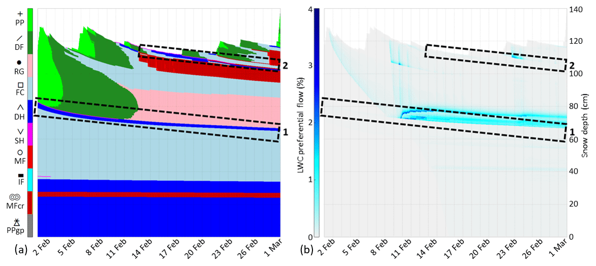
Figure 12 SNOWPACK simulation RE/PF/IceR in February 2017 at WFJ: (a) grain shape according to the classification of Fierz et al. (2009), and (b) liquid water content in the PF domain. Rectangles highlight layers 1 and 2.

Figure 13 shows the grain shape and the liquid water content in the matrix domain from 15 March to 15 April. A basal ice layer forms similarly to the RE/PF simulation. Contrary to the RE/PF simulation, the capillary barrier of layer 1 is still present (Fig. 13a). Melt forms appear at the layer transition from 22 March, and an ice layer forms in the matrix domain on 24 March, i.e., 4 to 5 d earlier than observed (Sect. 3.1.1 and 3.1.3). At this date, ice is transferred from the ice reservoir to the matrix domain (Fig. 14). The ice layer formed is 43 mm thick with a dry density of 821 kg m⁻³ and a significant volumetric liquid water content of θ_matrix=7.8 % and θ_PF=1.7 % (on 24 March 13:00 UTC). Similar to the RE/PF simulation, no ice forms at layer 2 due to the presence of melt-freeze crusts. However, fewer melt-freeze crusts are simulated in the snowpack, which is more in accordance with the observations. The matrix water flow reaches the ground on 30 March (Fig. 13b), i.e., 10 d before the observations (Sect. 3.1.2). The water front progression occurs too early, which is similar to the RE/PF simulations. The ice reservoir does not modify the snowpack runoff compared to the RE/PF simulations (not shown).

Figure 13 SNOWPACK simulation RE/PF/IceR from 15 March to 15 April 2017 at WFJ: (a) grain shape according to the classification of Fierz et al. (2009), and (b) liquid water content in the matrix domain. Rectangles highlight layers 1 and 2 with dashed lines before ice formation in the matrix domain and solid lines afterwards.

Figure 14 SNOWPACK simulation RE/PF/IceR from 15 March to 15 April 2017 at WFJ: volumetric ice content in the cumulated ice reservoir. Rectangles highlight layers 1 and 2 with dashed lines before ice formation in the matrix domain and solid lines afterwards.

3.2.3 Simulations over several winter seasons

To assess the impact of the ice reservoir parameterization on ice formation in the SNOWPACK model, simulations at WFJ are performed over 17 winters from 1999/2000 to 2015/2016 using the RE/PF and the RE/PF/IceR configurations. Only traditional snow profiles are available for evaluation, which is similar to Wever et al. (2016). Ice layers at the snow–soil interface are not taken into account because of the changing snowpack base in the observations over the winters (wooden board, gravel) and possible boundary effects in the simulations. Only simulated ice layers are verified against observations to calculate hits (number of simulated ice layers matching an observation) and false alarms (number of simulated ice layers that do not match any observation). A height difference of 20 cm is used for matching simulations and observations, which is similar to Wever et al. (2016). We assume that the formation date of an observed ice layer is between the last snowpack profile without an observed ice layer and the first profile where it is indicated. If the simulation date is more than 1 month away from the observed formation time interval or if the height difference is more than 20 cm, the event is considered a false alarm. Missed events (observed ice layers that are not simulated) are not counted. Indeed, attributing fortnightly visual ice observations to a unique observed ice layer can be very ambiguous and contrary to simulated ice layers that persist in time. Results of this multiyear evaluation are summarized in Table 1.

Table 1 Hits (HI) and False Alarms (FA) of simulated ice layers for RE/PF and RE/PF/IceR simulations at WFJ for 17 winter seasons from 1999/2000 to 2015/2016. HI (height and date): simulated ice layers that match an observed one formed at less than 20 cm of height difference and in the same time interval. HI (height only): simulated ice layers that match an observed one formed at less than 20 cm of height difference and less than 1 month away from the observed time interval. FA: simulated but not observed ice layers (or more than 1 month away from the simulated formation).

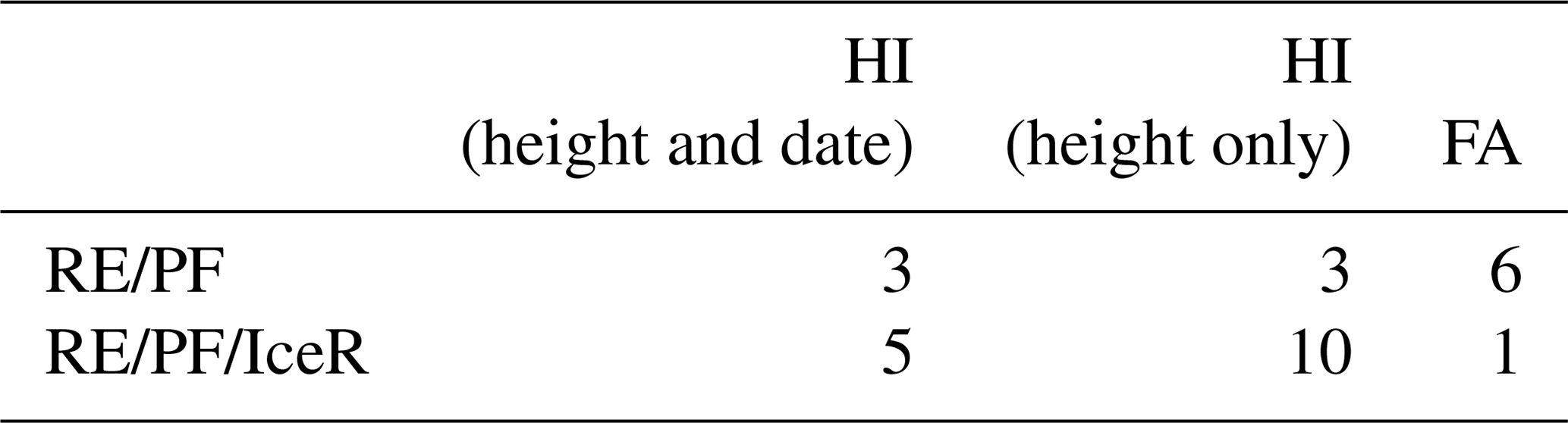
Overall, the addition of the ice reservoir parameterization to the RE/PF scheme enables it to form more ice layers with a higher number of hits (15 against 6, with a 1 month tolerance) and a lower number of false alarms (1 against 6). The simulated ice formation date is on average 22 d earlier than the observation interval for the RE/PF scheme and 4 d earlier for the RE/PF/IceR scheme. The premature ice formation with the RE/PF scheme is consistent with the overestimation of simulated early season snowpack runoff from preferential flow, as suggested by Wever et al. (2016). It is logically delayed in RE/PF/IceR simulations because the ice transits through the ice reservoir before being transferred to the matrix. The RE/PF/IceR configuration also mitigates the number of unobserved early melt-freeze crusts compared to the RE/PF configuration (not shown), as already highlighted for the 2016/2017 season (Figs. 10 and 12). However, a very high number of ground ice layers were simulated (17 for the RE/PF/IceR scheme against 8 for the RE/PF scheme). This number is probably excessive and due to possible snow-soil boundary effects.

4 Discussion

This detailed study of ice layer formation at Weissfluhjoch enables us to assess both a comprehensive observation dataset and state-of-the-art 1-D snowpack simulations for monitoring a complex process. We discuss hereafter the relevance of these methods and results.

First, the combined use of traditional snow profiles with measurements of higher temporal resolution like the SMP provides a suitable observation framework to study the transition period from dry to isothermal snowpack when ice formations appear due to preferential flow. Snowpack runoff measurements associated with snow temperature sensors and an upGPR-derived water front gave insights into the homogeneous wetting of the snowpack and the period when the bottom of the snowpack was primarily affected by preferential flow. SMP profiles of penetration resistance showed clear signals of the presence of ice, when compared to visual observations, with values higher than 10 N (Fig. 7), while penetration resistances in dry snow were mostly lower than 2 N (Fig. 6) and melt-freeze crusts were characterized by intermediate penetration resistances (usually between 5 and 10 N; Fig. 7). The identification of ice layers with several SMP profiles regularly spaced also offers a more quantitative estimate of ice heterogeneity than a subjective visual observation. However, the temporal and spatial variabilities may be complex to distinguish, as shown for layer 1 (Fig. 9). The visual layer tracking of SMP profiles is also a source of uncertainties. Hagenmuller and Pilloix (2016) developed a method matching several hardness profiles to synthesize them into one representative profile. This method was not considered relevant for the present study which focuses on the local heterogeneity of ice layers. Moreover, when ice layers are too thick, the SMP cannot go through them, as often happens in spring. For winter 2017 at WFJ, no complete SMP profile could be performed after 19 April. Finally, the difficulty in identifying the exact date of ice formation or attributing isolated, fortnightly ice layer observations in traditional snowpack profiles to a unique ice layer (Sect. 3.2.3) highlights the added value of the more comprehensive observation dataset used for winter 2016/2017. Overall, this comprehensive high-resolution dataset (also including detailed measurements of the density and specific surface area of the snow; Calonne et al., 2020) provides valuable information for a thorough validation of current and future snow-cover models.

The 1-D SNOWPACK simulations provide complementary insights into the observation dataset despite the spatial heterogeneity of ice layer formation due to preferential flow. The addition of an ice reservoir enables us to parameterize the local formation of ice at capillary barriers; it may thus be considered representative of the volumetric content of ice lenses at a given layer. These local specificities are not taken into account in the matrix domain, which is the mean state of the snowpack, until they become homogeneously spread. This parameterization, which delays microstructural changes in the matrix due to liquid water flow, is consistent with the recent findings of Hirashima et al. (2019) who showed that preferential flow paths migrate and thus gradually affect the original snow microstructure. Several limitations may be noted. The matrix flow modeled by the Richards equation occurs too early and leads to an excessive snowpack runoff, which is even more enhanced by preferential flow. This may explain the premature formation of ice layer 1; the matrix water front reaches this level on 24 March in simulations, while it is observed higher than 1 m on 24 March, and the surrounding layers are still dry on 28 March in the observations when the first ice lenses are observed. In addition, the performance of the RE/PF water transport scheme strongly depends on a good representation of the snow microstructure by SNOWPACK and particularly on the grain radius and snow density. For instance, no ice or water ponding are simulated at layer 2 during winter 2017 because the observed capillary barrier structure (rounded grains and faceted crystals above surface hoar) is not adequately represented (unobserved melt-freeze crusts above layer 2). Finally, the implementation of the ice reservoir is meant to improve the representation of ice formation within the 1-D framework of the RE/PF dual-domain approach, but it does not mitigate the limitations of the preferential flow parameterization. In particular, the vertical spreading of water flowing back from the preferential to the matrix domain is not solved; its effect on ice formation is only mitigated with the cumulated ice reservoir. Advances in preferential water flow modeling in the snowpack have recently been developed by Leroux and Pomeroy (2017, 2019) to tackle the capillary hysteresis effect and capillary pressure overshoot. They could be considered as improving the representation of preferential flow in the SNOWPACK model through a more accurate determination of capillary pressure at the tip of the preferential flow path with effects on the water transfer from preferential flow to the matrix domain.

Despite the limitations inherent to 1-D simulations of preferential flow, the dual-domain approach combined with the ice reservoir parameterization in SNOWPACK provides relevant information concerning deep ice layer formation. The ice reservoir limits the formation of unobserved early melt-freeze crusts and, overall, enables us to simulate more observed ice layers. For the detailed study of winter 2017, it gives complementary insights on the formation of ice layer 1; according to the simulations, the vertical preferential flow was sufficient to form the ice layer even though a possible contribution of lateral flow cannot be totally excluded.

5 Conclusions

We presented here a detailed study of deep ice layer formation in the snowpack due to preferential water flow at Weissfluhjoch, a high-altitude alpine site. Monitoring deep ice layers is of particular relevance for many applications but is challenging in natural snow conditions. This research proposed an approach based on the combined use of a novel comprehensive observation dataset at high temporal resolution and detailed snow-cover modeling with improved ice formation representation.

Weekly traditional snow profiles, snowpack runoff and temperature measurements, as well as upGPR-derived water front height, enabled us to better monitor the dry-to-wet transition period between mid-March and mid-April 2017. In particular, the first days of measured snowpack runoff could be attributed to preferential water flow, and the exact date of the first isothermal snowpack with matrix water flow reaching the ground could be identified. Daily penetration resistances measured with a SnowMicroPen (SMP) gave more accurate insights on ice layers, complementing the traditional visual observations. Through comparisons with the visual observations, penetration resistance thresholds of 5 and 10 N in SMP profiles could be defined for the identification of melt-freeze crusts and ice layers, respectively. Ice formation could be monitored at a higher temporal resolution, and the use of several profiles per day gave more quantitative information on the spatial discontinuity of ice. The daily succession of profiles also enabled us to track the two main capillary barriers where ice formed, providing additional information on the evolution of the layers.

The 1-D SNOWPACK simulations, including a parameterization of preferential flow, showed an overall good representation of the snowpack structure but a premature matrix wetting that is associated with an excessive snowpack runoff. The observed ice layers were not simulated due to the early formation of thick melt-freeze crusts, explained by limitations of the preferential flow scheme. We developed an ice reservoir parameterization to mitigate these limitations, with freezing water transferred from the preferential flow domain to an ice reservoir. The ice was included in the matrix domain when the layer could be considered to be continuous. This parameterization improved the simulation of winter 2017 with a limited number of unobserved early melt-freeze crusts and the formation of one ice layer. However, the early transition to a wet snowpack was not improved as the water transport was not modified. The ice reservoir scheme also showed improvements for the simulation of ice layers over past seasons.

These simulations highlighted the relevance of detailed snow-cover models for the modeling of complex phenomena like deep ice layers formed by preferential water flow since an accurate representation of the snow microstructure is necessary. Recent advances in preferential flow observations and modeling could contribute to strengthening water transport representation. This study also underlined the importance of comprehensive observation datasets for the validation of complex snow models. Collecting high-resolution data over more winter seasons will further improve the understanding of deep ice layer formation, particularly concerning their density, their impermeability and their evolution in the late melting season. Ice reservoir simulations also call for further experiments on large snowpack samples, similar to Yamaguchi et al. (2018), focusing on the formation of discontinuous ice lenses due to preferential water flow.