the Creative Commons Attribution 4.0 License.
the Creative Commons Attribution 4.0 License.
 | 09 Oct 2020
Impact of coastal East Antarctic ice rises on surface mass balance: insights from observations and modeling
Stef Lhermitte
Jan T. M. Lenaerts
Nander Wever
Mana Inoue
Frank Pattyn
Sainan Sun
Sarah Wauthy
Jean-Louis Tison
Willem Jan van de Berg
About 20 % of all snow accumulation in Antarctica occurs on the ice shelves. There, ice rises control the spatial surface mass balance (SMB) distribution by inducing snowfall variability and wind erosion due to their topography. Moreover these ice rises buttress the ice flow and represent ideal drilling locations for ice cores. In this study we assess the connection between snowfall variability and wind erosion to provide a better understanding of how ice rises impact SMB variability, how well this is captured in the regional atmospheric climate model RACMO2 and the implications of this SMB variability for ice rises as an ice core drilling site. By combining ground-penetrating radar (GPR) profiles from two ice rises in Dronning Maud Land with ice core dating, we reconstruct spatial and temporal SMB variations from 1983 to 2018 and compare the observed SMB with output from RACMO2 and SnowModel. Our results show snowfall-driven differences of up to 1.5 times higher SMB on the windward side of both ice rises than on the leeward side as well as a local erosion-driven minimum at the ice divide of the ice rises. RACMO2 captures the snowfall-driven differences but overestimates their magnitude, whereas the erosion on the peak can be reproduced by SnowModel with RACMO2 forcing. Observed temporal variability of the average SMBs, retrieved from the GPR data for four time intervals in the 1983–2018 range, are low at the peak of the easternmost ice rise (∼0.06 ), while they are higher (∼0.09 ) on the windward side of the ice rise. This implies that at the peak of the ice rise, higher snowfall, driven by orographic uplift, is balanced out by local erosion. As a consequence of this, the SMB recovered from the ice core matches the SMB from the GPR at the peak of the ice rise but not at the windward side of the ice rise, suggesting that the SMB signal is damped in the ice core.
- Article
(7119 KB) - Full-text XML
- BibTeX
- EndNote


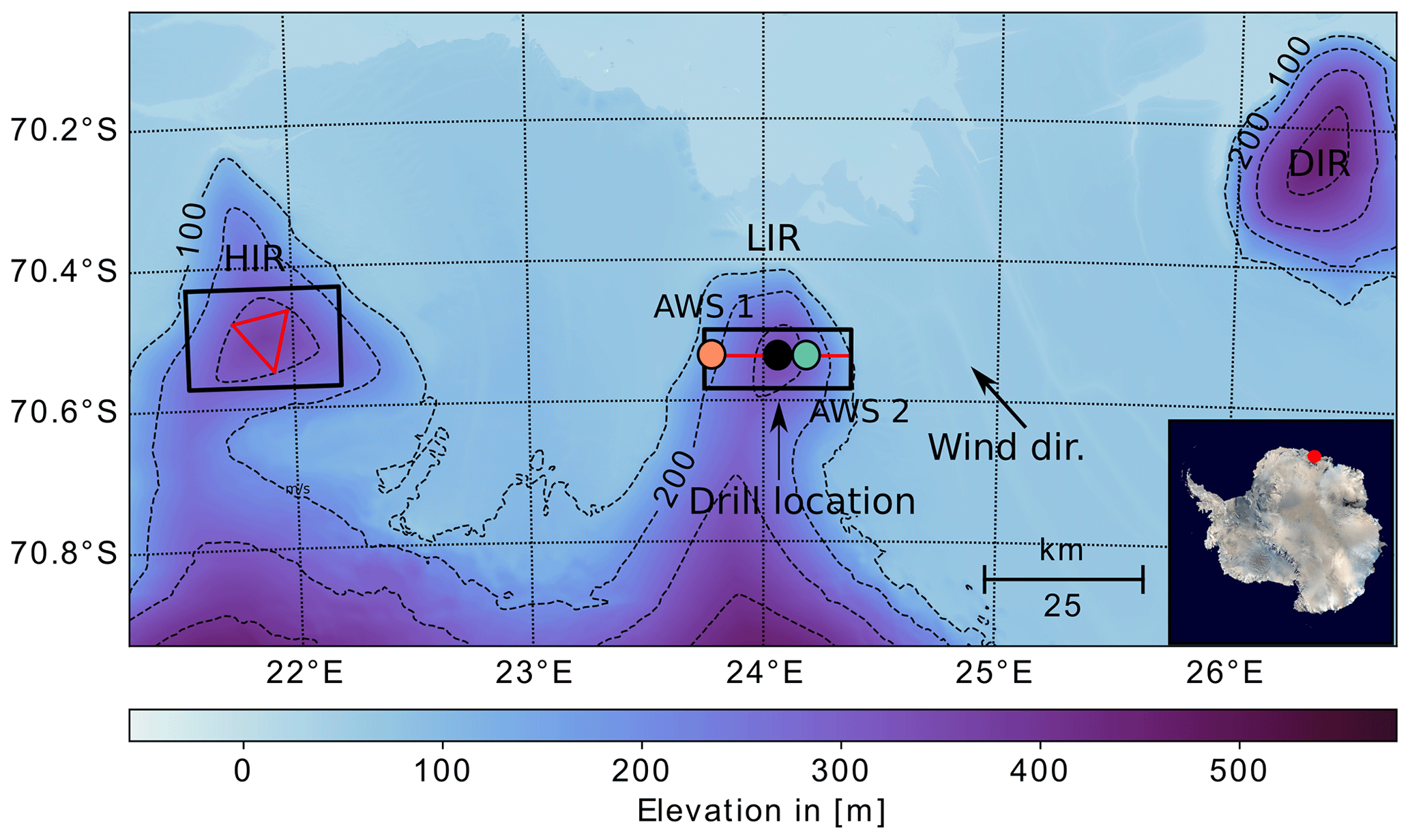
Figure 1Topography of the ice rise and the surrounding area in Dronning Maud Land, based on the 90 m TanDEM-X digital elevation model (© DLR 2018). The red lines represent the GPR profiles, the black boxes show the areas on which SnowModel was applied, and the two orange and green dots mark the locations of two AWSs installed on the eastern and western flank of the LIR. The bar plot in the lower left corner shows the wind speed and direction measured by the two AWSs between January 2018 and April 2018, where orange and green denote AWS 1 and 2, respectively.
The surface mass balance (SMB) remains one of the largest sources of uncertainty when determining the overall mass balance of Antarctica and with that Antarctica's contribution to sea level rise (Lenaerts et al., 2019; The IMBIE team, 2018; Rignot et al., 2019). The SMB of an ice sheet is commonly defined as the annual sum of all surface processes that affect the mass balance of an ice sheet. This includes snowfall, runoff of surface melt water, sublimation, drifting snow sublimation, and snow erosion and deposition, of which snowfall is the dominant component in East Antarctica (Boening et al., 2012). The SMB varies substantially in space across East Antarctica, with the highest SMB found on the coastal margins of the ice sheet and very low SMB on the East Antarctic Plateau, where the air is too cold to hold large amounts of moisture (Vaughan et al., 1999; Rotschky et al., 2007; Monaghan et al., 2006). The coastal regions of the East Antarctic Ice Sheet are characterized not only by high SMB but also by substantial interannual as well as spatial variability (Lenaerts et al., 2013, 2014).
Because of this high spatial and temporal variability, it remains challenging to determine changes in SMB of coastal East Antarctica in recent decades. For Dronning Maud Land (DML) alone, conflicting trends have been reported. For example Altnau et al. (2015) found a negative trend for the last 50 years for coastal DML using a compilation of firn cores, which matches with the results of Medley and Thomas (2019), who, even though their results show a generally positive SMB trend for East Antarctica, also found a negative SMB trend for coastal DML. On the other hand (Philippe et al., 2016) observed a positive SMB trend in a 120 m ice core in coastal DML for the last 50 years. Similar results were found by Thomas et al. (2017), who report a slightly positive trend for DML in the last 50 years, whereas the regional atmospheric climate model RACMO2 models no significant trend in the SMB for DML (Lenaerts et al., 2012b).
In order to understand these seemingly conflicting results, it is important to highlight and further investigate the high spatial SMB variability in DML. One of the main drivers for this spatial SMB variability are the numerous ice rises covering the coast of DML (Lenaerts et al., 2014). Ice rises are elevated local pinning points of the otherwise flat ice shelf, where the ice is grounded on topography and which are surrounded entirely (isles) or mostly (promontories) by the ice shelf (Matsuoka et al., 2015). Their topography influences the surrounding SMB by inducing snowfall, especially on the windward side of an ice rise, and by influencing the deposition of blowing snow by alternating the wind speed patterns (Lenaerts et al., 2014). In addition, ice rises are an ideal location to drill ice cores as they represent a local ice divide with low ice flow speeds (Matsuoka et al., 2015), which is necessary to recover past accumulation rates from a constant location in time. However, to interpret SMB rates recovered from ice cores, it is necessary to understand the impact of the ice rise on the regional and local SMB. There are two main processes by which ice rises control the SMB in coastal East Antarctica, which occur on different scales.
Firstly, in areas of steady winds, like DML, orographic uplift of moist air on upwind slopes of the ice rise leads to high snow accumulation on the windward side of the ice rise and a precipitation shadow on the leeward side of the ice rise (Lenaerts et al., 2014). This process occurs over the scale of the ice rise, which is typically 5–50 km wide in coastal East Antarctica. Here we define the scale from 5 to 50 km as the regional scale.
Secondly, local wind erosion and deposition of snow, especially around the peak of the ice rise, play a large role in the SMB distribution on the ice rise (King et al., 2004). This has been observed around local variations of the surface slope on a scale from 1 to 5 km (Black and Budd, 1964; King et al., 2004; Drews et al., 2015; Mills et al., 2019; Schannwell et al., 2019). Here we define the scale from 1 to 5 km as the local scale.
However, while both processes have been observed and modeled separately, not much is known about the relation between the two or about the importance of the two processes relative to each other. Here we aim to investigate this connection using the example of two ice rises in Dronning Maud Land (Fig. 1), with extensive field measurements as well as RACMO2, version 2.3p2 (Lenaerts et al., 2017; van Wessem et al., 2018) and the distributed high-resolution snow evolution model SnowModel (Liston and Elder, 2006). The field data were recorded during the 2017/2018 and 2018/2019 Mass2Ant field campaigns. Mass2Ant is an international project that aims to understand surface mass balance variability in space and time throughout coastal East Antarctica (Dronning Maud Land), with a focus on potential changes since 1850. The data used here include four ground-penetrating radar (GPR) tracks across two ice rises (Lokeryggen and Hammarryggen ice rises), hereafter referred to as the LIR and the HIR (Fig. 1), in the vicinity of the Belgian Princess Elisabeth Antarctica (PEA) station. Additionally, the field dataset includes data from two automatic weather stations (AWSs), installed on the eastern and on the western flank of the LIR, as well as an ice core at the center of the LIR and several firn cores along the GPR profile (Fig. 1). To connect the different scales we use the GPR data to reconstruct past accumulation rates across the two ice rises.
We combine the SMB reconstructed from the GPR data with the regional SMB distribution modeled by RACMO2 and the local SMB distribution over the ice rise modeled by SnowModel to quantify the magnitude of the local and regional effects on the SMB, what drives them and how well they are captured within the models. The goal of this study is twofold: (i) to reveal mechanisms that control the SMB on and around an ice rise and (ii) to better understand how SMB rates recovered from ice cores drilled into ice rises relate to the surrounding ice shelf.
2.1 Study area
The two ice rises are located in Dronning Maud Land in coastal East Antarctica close to the Belgian PEA station. Both ice rises are, to be specific, ice promontories and are surrounded by the ice shelf from the east, north and west and connected to the grounded ice sheet to the south (Fig. 1). The LIR is ∼350 m high and ∼25 km wide. It represents a local ice divide and neighbors the Roi Baudouin Ice Shelf to the east. On this ice rise, a 20 km east-to-west GPR profile was recorded during the 2017 Mass2Ant field campaign using a 400 MHz antenna (GSSI:SIR 3000). Along this profile, five firn cores were recovered to measure near-surface density variations in vertical direction. In addition, three 10 km GPR profiles were recorded during the 2018 Mass2Ant field campaign across the ice rise immediately west of the LIR, the HIR, which is ∼360 m high and ∼50 km wide and represents a triple junction for the ice flow (Fig. 1).
Additionally, an ice core was recovered at the center of the LIR, and two AWSs were installed on the western and on the eastern flank of the LIR (Fig. 1). The AWSs measured an average southeast wind direction of ∼132∘, which leaves the eastern flanks of the ice rises as the windward side and the western flanks of the ice rises as the leeward side.
2.2 Ice core data
A 208 m ice core (FK17) was drilled on the LIR (70.53648∘ S, 24.07036∘ E), during the 2017/2018 austral summer. We used the intermediate-depth ice core drill (ECLIPSE ice coring drill, Icefield Instruments, Inc.). A ∼2 m deep trench was excavated prior to drilling to allow the setup of the ECLIPSE ice core drill. To cover this part, a short core (∼9 m, FK18) was drilled during the following field season (2018/2019 austral summer). The cores were cut at a vertical resolution of 50 cm in the field to ease their processing. The ice cores were processed in a freezer laboratory at the Université libre de Bruxelles (Brussels, Belgium). The ice cores were cut in sticks with a clean bandsaw. The sticks ( cm) were used for trace ion measurement, and the outer part of the sticks was used for water-stable isotope measurement. Then the width, length and weight of the ice core sticks were measured 3 times and averaged to reconstruct the density profile. A total of 43 discrete sticks out of the top 125 m of the ice core were measured to obtain a density profile. Preliminary dating was achieved by counting the seasonal signal of the water-stable isotopes (δ18O and δD). Water-stable isotopes were measured using a cavity ring-down spectrometer (CRDS; Picarro, L 2130-i). Samples at 5 cm resolution were melted in a refrigerator prior to analysis. The values are expressed relative to the Vienna Standard Mean Ocean Water (VSMOW; Philippe et al., 2016; Inoue et al., 2017). Analytical precision for δ18O is <0.15 and for δD is <0.5 ‰. Note that this preliminary dating from the FK17 ice core needs to be further confirmed by multiple proxies such as trace ions (Na+, Cl−, non-sea-salt ). The annual snow accumulation record was obtained from the thickness of annual layers after ice core dating was done. The thickness of the annual layers was converted into meters of water equivalent using the density measurements of the ice core.

Figure 2(a) Interpolated surface density, (b) GPR profile across the LIR from west to east (red line on the LIR in Fig. 1) and (c) the modeled density curves together with measured density from the FK17 ice core. The surface density is linearly interpolated from firn core measurements; the black diamonds mark the location of the firn cores. The black lines in (b) show the three tracked horizons together with their dating, and the vertical black line shows the location of the FK17 ice core.
2.3 SMB from ground-penetrating radar
To study the spatial SMB distribution across the ice rise, we used a GPR. The GPR emits radar beams into the ground and records the time it takes for the signal to return after being reflected from internal layers within the snowpack. These internal reflection horizons (IRHs) are created by changes in conductivity, density and ice crystal orientation and represent former surface layers (Spikes et al., 2004; Fujita et al., 1999; Callens et al., 2016). The two-way travel time of the signal is then converted into depth by multiplying it with the radar beam velocity within the snowpack and dividing by 2. Here we employed a 400 Mhz antenna, dragged behind a Ski-Doo to survey the shallowest 50 m of the snowpack.
To reconstruct the SMB out of the GPR data, we used the shallow-layer assumption, in which snow accumulation and densification control the IRHs in the upper layers of the snow column, while vertical strain plays a larger role in the deeper layers (Waddington et al., 2007). Following this assumptions one only needs the depth of an IRH, the age of the IRH and the density profile with depth to calculate the average SMB. This is because the depth of the IRH layer tracked through the GPR profile provides information about the volume of snow which accumulated since the IRH formed the surface of the snowpack. Combined with the layer age information, this provides the volume of snow accumulated in a certain time frame. If additionally the density distribution with depth of the snowpack is known, it is possible to calculate the snow mass which accumulated since a certain point in time with the layer age information from the ice core. This value can be interpreted as the average SMB over the time period as SMB is a measure of snow mass accumulated per year.
To obtain the depth and age of the IRHs as well as the density distribution with depth for the profile across the LIR, we followed a stepwise process. The goal of this process is to reconstruct the average SMB across the profile for three time periods within the last 40 years.
-
The first step was to obtain the density distribution with depth as this is needed to (a) calculate the SMB from the layer depth and (b) calculate the increase in radar velocity with depth. In order to get the density distribution with depth, we used the Herron–Langway (Herron and Langway, 1980) firn densification model. The model requires surface density, average surface temperature and average accumulation rates as input. We used the surface density from firn cores along the GPR profile and interpolated that linearly (Fig. 2a). For the average surface temperature −17 ∘C was used, which is the average surface temperature of the last 36 years according to RACMO2. For the average accumulation rates we used an iterative procedure, where we first set the accumulation to 0.55 across the whole profile and then used the results of the first run as input for the second. This way we created an ensemble of 220 density curves along the GPR profile, one for every 100 m, to account for lateral changes in the density distribution with depth. The modeled density curves are in good agreement with the densities measured in the FK17 ice core in the center of the ice rise (Fig. 2c).
-
The second step was to trace three IRHs and date them using the age information of the 2017 Mass2Ant ice core in the center of the GPR profile (Fig. 2). The deepest IRH represents the surface from 1983, followed by the IRH representing 1994 and 2002. This layer depth was calculated from the two-way travel time using a radar velocity which increases with density following the mixing formula of Looyenga (1965). The combination of tracked layers and ice core provide the depth and age information for the SMB.
-
Finally we combined the density model, one layer depth value for every 100 m along GPR IRHs and the age dating from the ice core to calculate 220 SMB values for each time interval along the profile (Fig. 3b). Each SMB value was calculated by summing up the density between two IRHs and dividing by their age difference.
where ρ(z) is the density at depth z, Ve=1 m3 is a volume element, di is the depth of an IRH, and Ai is the age of the respective IRH. The error bars around the SMB profile represent the uncertainty due to the age measurement and the density model.
For the three profiles across the HIR (Fig. 3), a different approach without dating the tracked IRHs was used as there is not yet age information for the IRHs available as of the time of writing this study. Due to the lack of dating information, we worked with the relative spatial SMB distribution across the ice rise, which is independent of the age information. This was accomplished by tracking one continuous IRH across all three adjacent/connected profiles (Fig. 3) and assigning it the age of its average depth according to the 2017 ice core recovered at the LIR. To address the potential uncertainty as a result of this relative approach, we introduced an uncertainty of ±5 years to the age. Additionally, due to a lack of surface density measurements recorded at the HIR profiles, we set the surface density to the average value of 400 kg m−3 for the Herron–Langway density model. Consequently the SMB profiles 2, 3 and 4 across the HIR (Fig. 3d–f) can only be interpreted in terms of their relative SMB variations across the profiles while disregarding their absolute values. However, since the three profiles on the HIR are connected in a triangle, it was possible to trace the same IRH through all of them and spatially interpolate the SMB within the triangle (Fig. 3c).
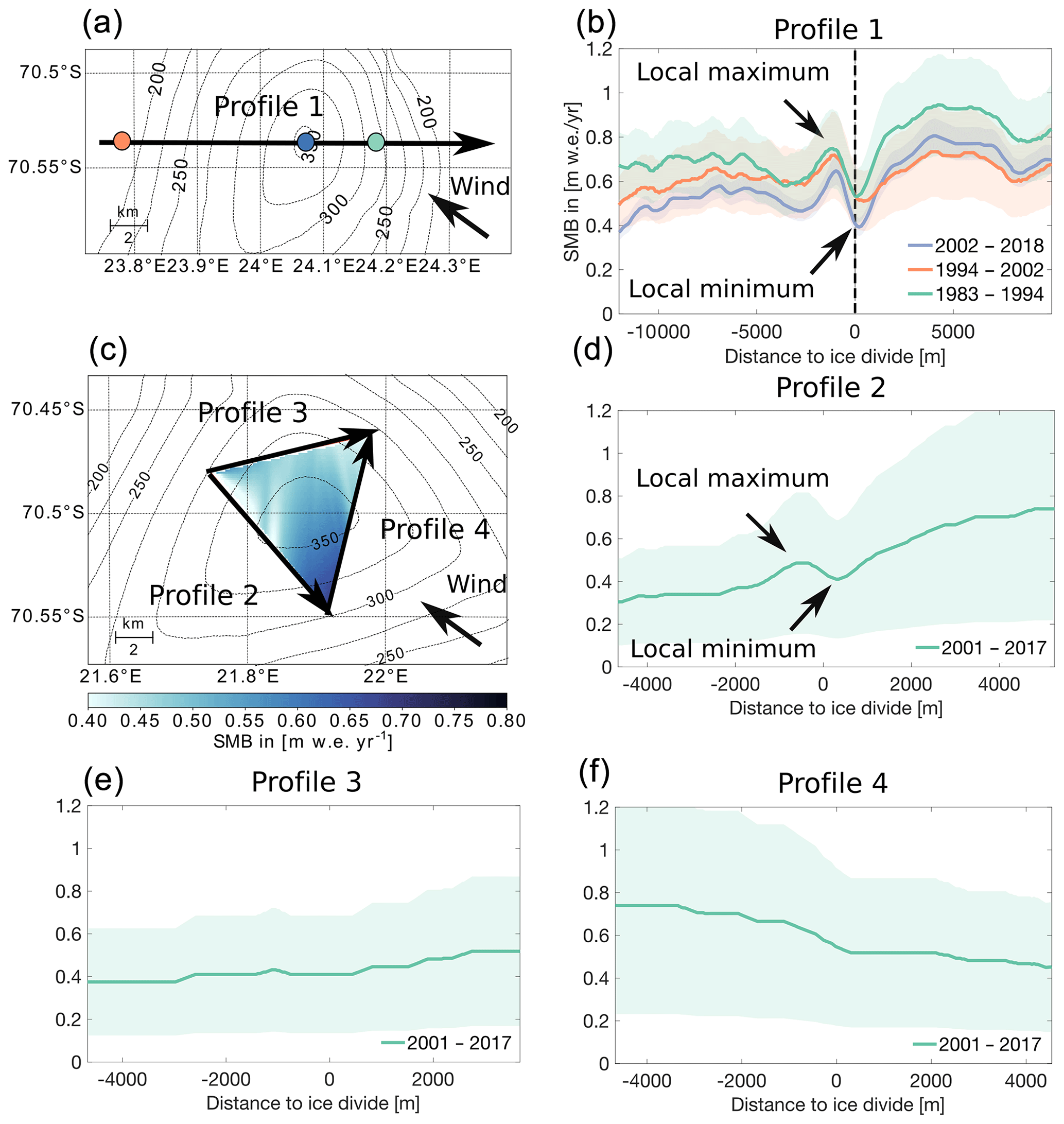
Figure 3Topography of the LIR, the location of the two AWSs (green and orange dots), the drilling site of the FK17 ice core (blue dot) and the GPR tracks recorded during the 2017 Mass2Ant field campaign (a). Also shown is the SMB reconstructed from the GPR profile on the LIR (b) as well as the topography and the GPR tracks on the HIR (c), where three SMB profiles were reconstructed from GPR profiles for a single time window (2001–2007) by tracking a single IRH of age deduced from the depth–age relationship at the LIR ice core (d, e, f). The topography of the ice rises shown in (a) and (c) is based on the 90 m TanDEM-X digital elevation model (© DLR 2018).
2.4 RACMO2
RACMO2 is a state-of-the-art regional atmospheric climate model. Similar to, for example, MAR (Agosta et al., 2019) and COSMO-CLM (Souverijns et al., 2019), it is able to provide accurate SMB simulations in polar regions. RACMO2 was developed by the Royal Netherlands Meteorology Institute (KNMI) and combines the High Resolution Limited Area Model (HIRLAM; Undén et al., 2002) numerical weather prediction model with the European Centre for Medium-Range Weather Forecasts Integrated Forecast System (IFS) physics (ECMWF, 2009; Noël et al., 2015; Lenaerts et al., 2012b). Here we are using the latest version, RACMO2.3p2, for Antarctica (van Wessem et al., 2018). RACMO2.3p2 includes a multilayer snow model that simulates the effect of heat diffusion, compaction, melt water percolation, retention and refreezing, and grain size evolution on the surface temperature and albedo. Furthermore, a bulk snowdrift model is embedded in RACMO2 (Lenaerts et al., 2012a). Here, data from a 5.5 km resolution simulation for East Antarctica covering the time span of 1979–2016 are used, of which we used the time period from 2011 to 2016.
2.5 SnowModel
SnowModel is a distributed snow evolution model (Liston and Elder, 2006). It consists of four connected modules, which model and spatially interpolate the meteorological input quantities (MicroMet), the energy balance (EnBal), the evolution of the snowpack (SnowPack), and the redistribution of blowing snow by erosion and deposition (SnowTran-3D). The spatial interpolation of the meteorological input data follows the Barnes objective-analysis scheme, which uses a Gaussian weighted average technique (Koch et al., 1983). SnowPack simulates the changes in snow depth for multiple snow layers but does not consider any snow microstructure. Here we ran SnowPack with a single snow layer for simplicity reasons. SnowTran-3D updates this snow depth depending on the amount of saltation, suspension and blowing snow sublimation (Liston and Sturm, 1998). The spatial resolution of SnowModel is limited by the spatial resolution of the digital elevation model (DEM). Here we used the TanDEM-X 90 m DEM (Lenaerts et al., 2016).
In terms of meteorological input, SnowModel relies on time series of five quantities: air temperature, relative humidity, wind speed, wind direction and snowfall for at least one point within the area of interest. Daily RACMO2 data from the grid cells surrounding the locations of the two AWSs were used as meteorological input for SnowModel.
In addition to the DEM and the meteorological variables, SnowModel requires a number of additional input parameters. The most consequential ones are the curvature length scale (distance over which curvature is calculated) of the topography, the weighting between curvature and slope for the wind model, the threshold shear velocity, and the roughness length. Regarding the weighting between curvature and slope, we focused on the effect of the curvature on the wind field, setting the curvature weighting to 1.0 and the slope weighting to 0.0. We did this to focus on processes located at the peak of the ice rise, where the ice core was drilled. At this part of the ice rise the curvature is large, while the slope is 0. For the curvature length scale we used 100 m. Another important input parameter is the roughness length, which together with the threshold shear velocity determines the wind speed necessary to create erosion. The roughness length describes the theoretical height above the surface, where the wind speed would reach 0 (Blumberg and Greeley, 1993). For both the roughness length and the threshold shear velocity, we tried different values using forward modeling. We varied the roughness length between 0.05 and 0.00005 m and the threshold shear velocity between 0.3 and 0.8 m s−1 and chose the values which qualitatively fit the reconstructed SMB values from the GPR best. This was achieved with a roughness length of 0.005 m and 0.6 m s−1 for the threshold shear velocity. Even though the chosen roughness length is an order of magnitude larger than typically reported for the Antarctic ice sheet (König-Langlo, 1985; Bintanja and Van Den Broeke, 1995) in wind-erosion-dominated environments with large sastrugi forming, larger roughness lengths have been found (Amory et al., 2017). Clifton et al. (2006) observed a strong relationship between threshold shear velocity and snow density, where values larger than 0.6 would be expected for the threshold shear velocity for a near-surface snow density of above 300 kg m−3. Combined with the chosen roughness length, a threshold shear velocity of 0.6 m s−1 results in 10 m threshold wind speeds of around 11.4 m s−1 to initiate erosion. Based on the frequency with which RACMO2 simulated wind speeds exceed 11.4 m s−1 for the ice rise and the frequency with which wind speeds observed by the AWS exceed 11.4 m s−1, we estimated that with those settings, we have an appropriate representation of erosion frequency in SnowModel. Between January and April 2018 the AWS on the windward side measured daily wind speeds exceeding 11.4 m s−1 50 % of the days. This is in agreement with observations from Amory (2020), who observed similar erosion frequencies between January and April for a site in coastal Adélie Land with a comparable elevation of 450 m.
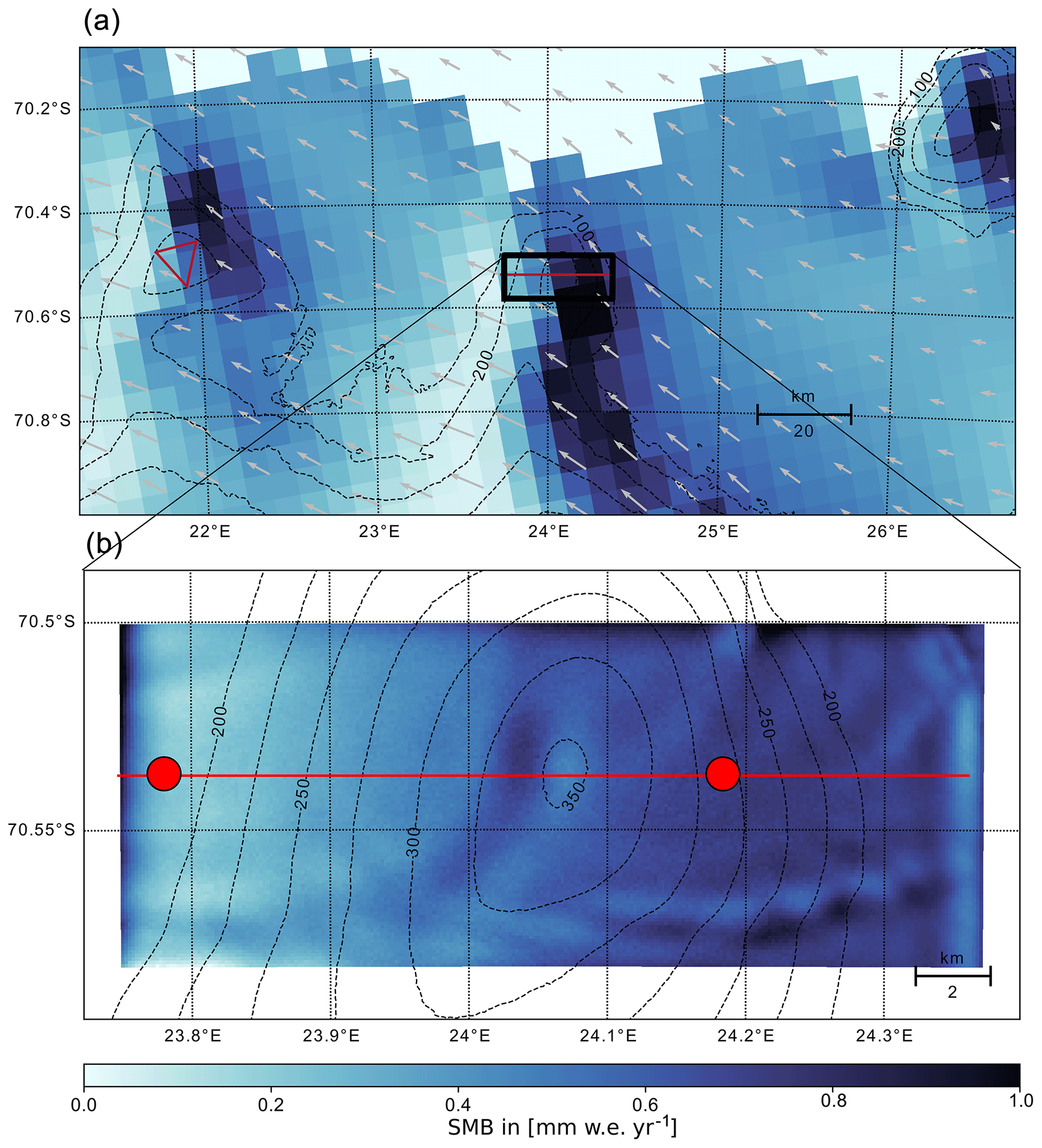
Figure 4Overlays of the SMB modeled by RACMO2 (a) and SnowModel (b) for the time period of 2011 to 2017 with topography contour lines based on the 90 m TanDEM-X digital elevation model (© DLR 2018) and RACMO2 wind vectors (gray arrows). The simulated area by SnowModel is marked in (a) with a black box. The red lines show the location of the recorded GPR tracks.
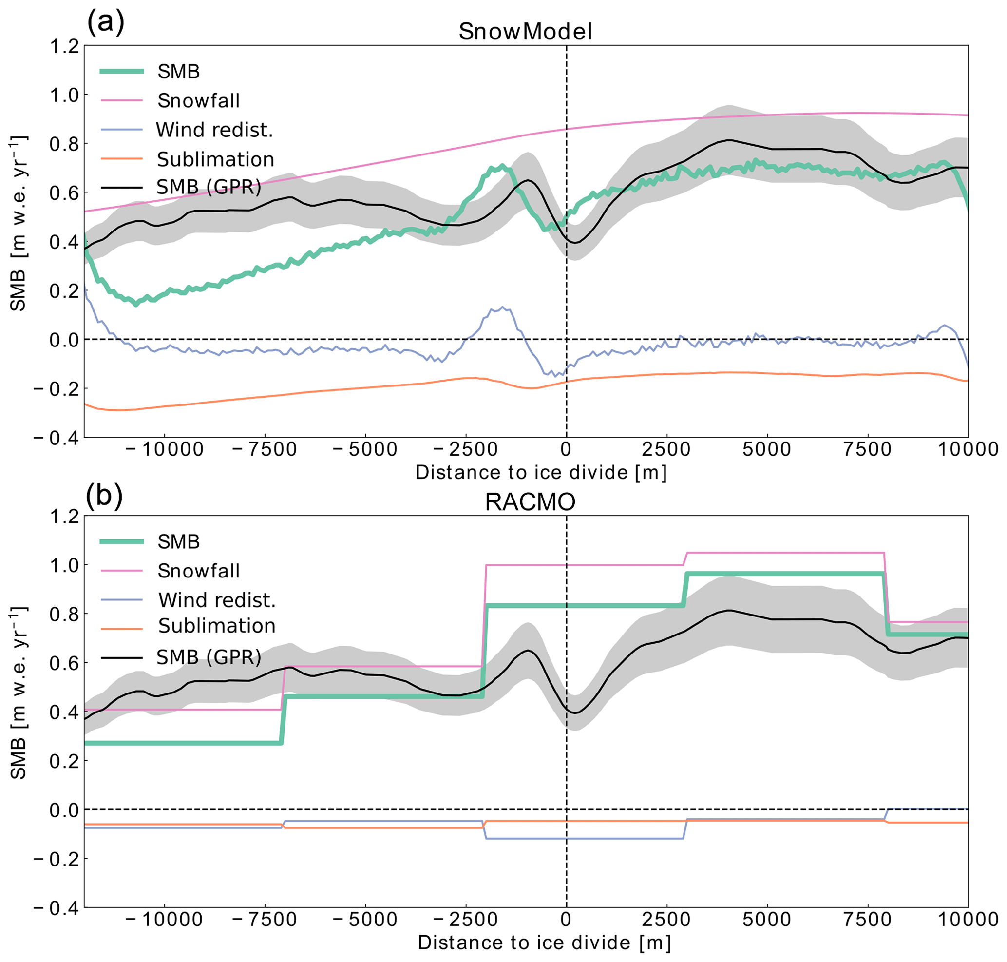
Figure 5Profiles showing the total SMB and the different components of the SMB across the west-to-east profile of the LIR modeled by (a) SnowModel and (b) RACMO2. SMB reconstructed from the GPR data is also shown together with an estimated error in light gray. The location of the profile is shown in Fig. 4.
3.1 Regional surface mass balance around the ice rises
To investigate the regional SMB around the ice rises, we utilize the SMB reconstructed by the GPR data (Fig. 3) as well as the SMB modeled by RACMO2 (Fig. 4). Both SMB datasets qualitatively agree on the SMB variability over the ice rises but differ on the amount and the contrasts between windward and leeward sides. For our region of interest in Dronning Maud Land (the whole extent of Fig. 4a), RACMO2 models an average SMB of ∼0.35 across the ice rises and ice shelf. However, along the windward flanks of the LIR, the HIR and the Derwael Ice Rise (DIR; Norwegian: Kilekollen), the modeled SMB values are substantially higher, around ∼1.0 (Fig. 4). These high SMB values on the windward flanks of the ice rises are accompanied by low SMB values on the leeward flanks of the ice rises around ∼0.2 . We can observe a similar SMB difference across the LIR in the SMB reconstructed from the GPR data. The GPR profile across the LIR (Fig. 3) shows SMB values between 0.4 and 1.0 , with an average SMB across the ice rise of ∼0.7 in the period of 1983 to 1994 and ∼0.6 between 1994 and 2002 as well as ∼0.6 in the most recent time period of 2002 to 2018. The SMB values for all three time periods are consistently higher on the windward side of the ice rise than on the leeward side of the ice rise (Fig. 3b). This windward–leeward difference is largest between 2002 and 2018, with an average SMB difference of ∼0.2 and the lowest in the period of 1994 and 2002, with ∼0.1 . However, while RACMO2 models a ∼5 times higher SMB on the windward side of the LIR than on the leeward side, the GPR profile 1 across the LIR measures at most a ∼1.5 times larger SMB on the windward side of the ice rise than on the leeward side (Fig. 5). That implies that for LIR, the difference in SMB between windward and leeward side is considerably larger in RACMO2 than in the observations (Fig. 5). This is in agreement with Agosta et al. (2019), who found that RACMO2 indeed overestimates snowfall on the windward side of topography. However, the average SMB across the ice rise (parallel to profile 1 of Fig. 3) in RACMO2 is similar to the SMB from the GPR for the observed time period of 1983 to 2018, with ∼0.54 and ∼0.7 , respectively.
For the HIR, RACMO2 models between ∼2 and ∼2.40 times higher SMB values on the windward side of the ice rise than on the leeward side. This difference is stronger in the north of the ice rise, where SMB values are around ∼0.6 , and lower in the south, where SMB values are around ∼ 0.5 (Fig. 4). Here the SMB reconstructed from the GPR data shows a similar difference of ∼2 times higher SMB values on the windward side than on the leeward side, but in contrast to RACMO2 (Fig. 4a) the highest values are found in the southeast of the ice rise instead of the northeast (Fig. 3c). Now one would intuitively expect SMB to be highest in the southeast sector of the ice rise, where rising air provides enhanced precipitation.
In general, the regional difference in SMB between the windward and the leeward side of the LIR seems to be largely driven by a difference in snowfall. We can observe this in the distribution of the modeled SMB components across the ice rise (Fig. 5a). In Fig. 5a we see that the SMB curve across the ice rise largely follows the snowfall curve. Sublimation and wind redistribution also play a role for the SMB, but sublimation is relatively constant in space and does not seem to contribute to the SMB difference between the windward and the leeward side of the ice rise. Wind erosion also seems to only play a negligible role in creating the large-scale SMB difference between the windward and the leeward side of the ice rise (Fig. 5) as RACMO2 models relatively constant erosion across the whole ice rise. In RACMO2, this eroded snow is then deposited downwind of the ice rise on the surrounding ice shelf (Lenaerts et al., 2014). However, with sublimation and wind redistribution being relatively constant across the LIR, the difference in snowfall seems to be the controlling factor for the difference in SMB. This confirms the narrative that the large-scale difference in SMB is a result of orographic precipitation on the windward side of the ice rise (Lenaerts et al., 2014).
3.2 Local surface mass balance at the ice divide
Local minima in SMB can be identified in the GPR data at the ice divide (the highest point of the ice rise) as well as local SMB maxima within the first 2000 m west of the ice divide in the SMB profile across the LIR (Fig. 3b). These large amplitudes in the GPR layers may be the result of accumulation differences and therefore represent local SMB differences, but they may also be the result of internal ice deformation resulting from higher vertical velocities at the flow divide compared to the flanks, the so-called Raymond effect or Raymond bump (Raymond, 1983). To test whether or not this anomaly around the peak of the ice rise is an accumulation feature controlled by the SMB or the result of the Raymond effect, we used a technique described by Vaughan et al. (1999). If the amplitudes of the arches in the GPR data increase linearly in size with depth, it is the result of snow accumulation, whereas if the amplitudes increase quadratically, it is the result of internal deformation (Raymond effect). As shown in Fig. 6, the amplitudes in our data increase linearly in size with depth for profile 1 and are therefore interpreted as a result of accumulation. This argument is supported by the results of Drews et al. (2015), who applied the same method at the neighboring DIR and also came to the conclusion that the shallow arches found in their GPR data are a result of accumulation differences and not internal deformation.
This anomaly of low SMB at the divide and high SMB west of it is consistent through all three time periods observed at the LIR and has an average amplitude of ∼0.2 . The SMB values at the ice divide are ∼0.4 during the most recent time period of 2002 to 2018, ∼0.5 from 1994 to 2002 and ∼0.5 from 1983 to 1994. These values agree with the average accumulation rates for the same time periods determined from the ice core at the center of the ice rise of ∼0.40, ∼0.50 and ∼0.48 , respectively (Fig. 7). We also observe a similar SMB minimum at the ice divide in profile 2 across the HIR as well as a local SMB maximum within 2000 m downwind of it. However, there the SMB minimum is ∼500 m southeast of the ice divide (Fig. 3d). The SMB varies by ∼0.1 between the minimum at the divide and the downwind maximum, which is substantially smaller than at the LIR. In addition to this, the anomaly is only present in profile 2 of the three profiles across the HIR (profiles 2, 3, 4; Fig. 3) even though all profiles cross a local ice divide.
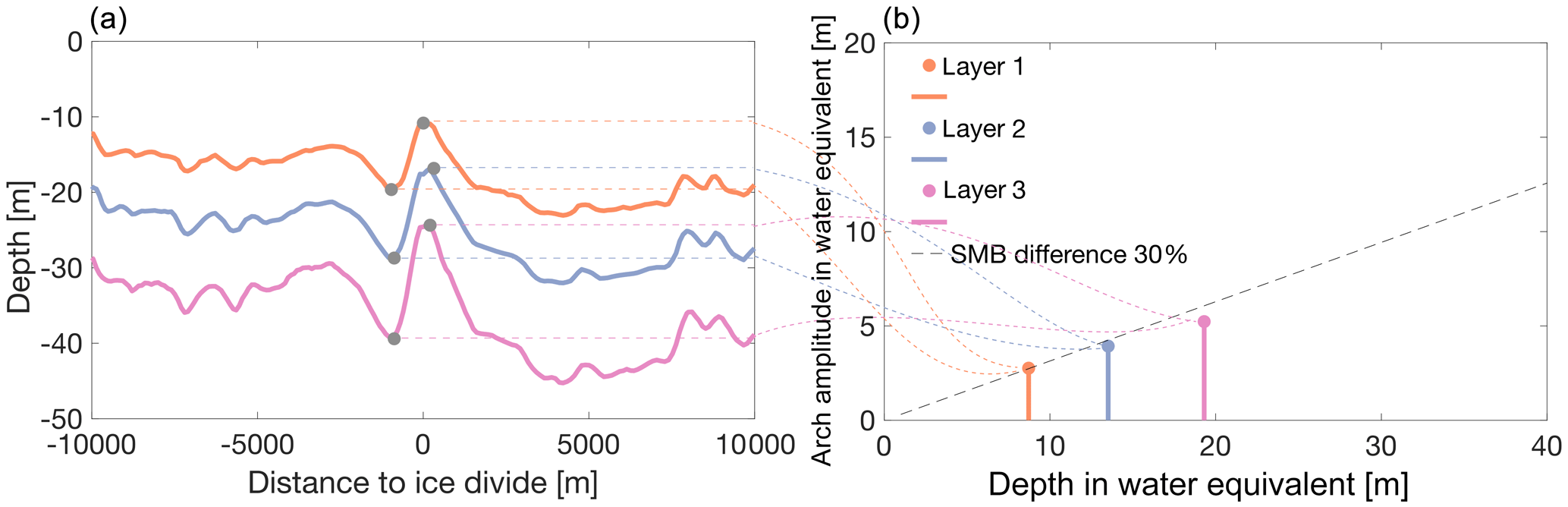
Figure 6Panel (a) shows the depth of the tracked IRH from the GPR data (Fig. 3) across the LIR. Panel (b) shows the arch amplitudes around the ice divide (in water equivalent) versus the depth of the arches. The dashed line shows the theoretical size of the arch amplitudes with depth for an SMB difference of 30 %.
To investigate the role of snow redistribution by wind, we use SnowModel with RACMO2 forcing for the area on the LIR. SnowModel reproduces the anomaly of low SMB on the peak of the ice rise and a local maximum west of the peak (Fig. 5). Furthermore, SnowModel provides the individual SMB components, which reveal that this anomaly in the SMB is a result of high negative wind redistribution (erosion) at the peak and high positive wind redistribution (deposition) within the next 2 km west of the peak. This indicates that snow is eroded at the top of the ice rise, where wind speeds are high, and deposited within 2 km leeward of the ice divide. This is in agreement with the observations made by King et al. (2004), who observed similar local SMB variations across the Lyddan Ice Rise in Antarctica and explained them as a result of snow redistribution by wind. The absence of the local minima at the ice divide on profiles 3 and 4 across the HIR (Fig. 3) provides further evidence that this is a wind-driven accumulation feature and not a result of internal deformation. All three profiles cross one of the ridges of the ice rise at a similar elevation; however, only the one parallel to the dominant wind direction (profile 2) shows the local SMB minimum and maximum near the peak of the profile (Fig. 3). Therefore, it seems that positive curvature of the topography, parallel to the dominant wind direction, is necessary to create this erosion and deposition feature.

Figure 7The SMB in time recovered from the FK17 ice core (dashed black line) as well as the SMB recovered from the FK17 ice core averaged for the three time periods (1983–1994, 1994–2002, 2002–2015; solid black line). The solid orange line is the SMB for the same three time periods reconstructed from GPR profile 1 at the peak of the LIR, whereas the solid pink line is the average SMB on the windward side, the light green solid line is the average SMB on the leeward side, and the blue line is the average SMB across the whole GPR profile 1 for the same three time periods.
Overall the SMB of an ice rise seems to be controlled by two different mechanisms: a larger-scale systematic difference of higher snowfall at the windward side of an ice rise, which affects the SMB of the ice rise as a whole, and a localized effect of wind erosion and deposition around the peak of the ice rise. This is in agreement with Drews et al. (2015), who observed similar effects on the neighboring DIR, explaining the large-scale difference as a result of higher snowfall on the windward side and suggesting wind redistribution as a driving force of the small-scale variations. However, they mention that this might not be a generic ice rise feature as Vaughan et al. (1999) and Conway (1999) did not find any evidence for wind erosion at Fletcher Promontory and Roosevelt Island, respectively. However, those studies used low-frequency radar with high penetration depth to investigate internal structures within the ice, which consequently had low resolution near the surface such that it is possible that the effect of wind erosion on the peak of the ice rise was not resolved. Since we found these effects to occur on both ice rises, congruent with studies from other locations (Derwael and Lyddan ice rises; Drews et al., 2015; King et al., 2004), we conclude that these features are likely generic for ice rise features in at least East Antarctica, possibly all of coastal Antarctica.
To investigate the implications of these two processes for ice rises as ice core drilling locations, we can compare the SMB recovered from FK17 to the SMB from GPR across the LIR and to the SMB form the GPR at the location of FK17. The ice core at the center of the LIR yields an average SMB of ∼0.45 between 1983 and 2015. This is in agreement with the average SMB reconstructed from the GPR at the ice core location of ∼0.5 for the same time period (Fig. 7). However, as we showed earlier, the center of the ice rise is affected by substantial erosion. This results in the SMB being lower at the ice core location than the average SMB of the ice rise across profile 1 for the same time period, which is ∼0.7 . However, the average SMB along profile 1 of the LIR is substantially larger than the general SMB of the surrounding ice shelf due to the high amount of snowfall on the windward flank of the ice rise. Even the average SMB values on the leeward side of the LIR of ∼0.6 are still well above what RACMO2 models for the average SMB of the surrounding ice shelf area, with ∼0.35 . So unlike in RACMO2, where SMB values are as low as ∼0.27 on the leeward side of the ice rise, we do not observe a strong precipitation shadow on the leeward side of the LIR in the GPR data. This means that the peak of the ice rise represents the location within GPR profile 1 where the reconstructed SMB is closest to what one would expect for the surrounding ice shelf. Therefore, in the case of the LIR, it seems like the erosion at the ice divide partially cancels out the higher SMB values due to orographic uplift and results in an overall lower SMB at the ice core location, which better resembles the surrounding shelf.
This is likely a generic feature for ice rises of all shapes as the orographic enhanced precipitation scales with the slope of the ice rise, the erosion at the peak of the ice rise scales with the curvature of the ice rise, and both processes are generally opposed to each other. However, the magnitude of each process individually might vary strongly between ice rises as both processes also scale with other factors like wind speed and atmospheric moisture content in addition to the topography.
The observed difference between the local SMB minimum at the peak of the ice rise, where the snow gets eroded, and the SMB maximum just downwind of the peak, where the snow gets deposited, is very large at the LIR (∼0.2 ) compared to the neighboring HIR and DIR. At both of these locations, this erosion and deposition feature has an amplitude of ∼0.1 . Surprisingly this is the case despite the generally lower average wind speeds of ∼8.8 m s−1 across the LIR compared to ∼9.6 m s−1 across the HIR (according to RACMO2). Also at the LIR, the erosion and deposition feature was largest in the time period from 2002 to 2018, when the average wind speed was slightly lower than from 1983 to 1994 and 1994 to 2002, according to RACMO2. Therefore it seems that wind speed is not the only determining factor for the local erosion feature.
Theoretically erosion occurs if the local wind speed exceeds a certain wind speed threshold, which in itself depends on the surface roughness length and the threshold shear velocity (Clifton et al., 2006). In addition it seems that threshold shear velocity is largely dependent on near-surface snow density (Clifton et al., 2006). Therefore a possible explanation for the higher erosion at the LIR could be that the magnitude of the erosion feature depends on the overall snowfall, where higher snowfall would create larger erosion by enhancing the availability of fresh low-density snow, which in turn is easier to erode as it has a lower threshold shear velocity. However, in SnowModel the threshold shear velocity does not change with snowfall, and more advanced models (e.g., Alpine3D; Lehning et al., 2006) which include snow microstructure would be necessary to model the effect of a changing threshold shear velocity with snowfall. In fact, there is observational evidence for an increase in erosion with snowfall. For example a recent study by Souverijns et al. (2018), who used a set of remote-sensing instruments at a study site close to PEA station, found that snowfall events only led to accumulation 60 % of the time, while leading to ablation 40 % of the time due to the erosion of the freshly fallen snow, and confirmed earlier studies in that the availability of fresh snow is more important for erosion to occur than high wind speeds (Gallée et al., 2001).
Another indicator for the increase in erosion with snowfall is that the SMB variability on the windward side of the LIR between the three observed time periods is higher (∼0.09 at maximum) than the temporal SMB variability at the peak of the ice rise (∼0.06 at maximum). This would imply that locally, around the peak of the ice rise, the regional processes of high SMB on the windward side due to higher snowfall would be partially canceled out by the erosion process. A consequence of this is that the absolute accumulation values measured from the ice core at the peak of the ice rise resemble more closely the SMB values expected for the surrounding ice shelf but also that they show less sensitivity to the temporal snowfall variability on the ice rise itself. This becomes evident when looking at the temporal SMB evolution on the windward side of the ice rise compared to the SMB evolution at the peak of the ice rise or the leeward side (Fig. 7). While the SMB at the peak of the ice rise and on the leeward side decreases with time, the SMB on the windward side decreases only until 2002 but then increases in the latest time period, from 2002 to 2018. This shows a disconnect between the SMB evolution at the peak of the ice rise (where the ice core is recovered) and the windward side of the ice rise, where snowfall is highest. Now since we observe high SMB on the windward side of an ice rise and erosion at the peak of an ice rise on other ice rises too, it is not unlikely that this disconnect between SMB evolution at the peak and on the windward side is also a generic ice rise feature. A consequence of this would be that an SMB record from an ice core at the peak of an ice rise alone would only be sufficient to derive the SMB at the very peak of the ice rise and the leeward side but would fail to capture the SMB evolution on the windward side of the same ice rise. However, for now we have only observed this at the LIR since we do not have a temporal resolution for the HIR data to test this in more detail. More observations at other ice rises, where GPR data and ice core data are combined, would be needed to confirm this hypothesis. A possible candidate for this would be the neighboring DIR, where all these datasets were collected. In any case our results highlight the value of GPR data around an ice core to put SMB values recovered from the ice core into context.
Here we combine in situ GPR measurements and ice core data with state-of-the-art modeling results to investigate the spatial variations across two ice rises in Dronning Maud Land as well as the spatial and temporal variations across one of the ice rises for the time period of 1983 to 2018. We identify two main processes which influence the SMB across the ice rises: a regional snowfall-driven process of higher SMB on the windward side of the ice rises due to orographic uplift and a local wind-driven erosion process, where snow is eroded at the peak of the ice rise and deposited within a couple of kilometers downwind of the peak. At the LIR, where we have both GPR data and an ice core available, the SMB reconstructed from the GPR shows that both processes play a role for the SMB at the drilling location. For this ice rise the erosion at the peak of the ice rise locally evens out the higher snowfall values on the windward side of the ice rise. Not only does the erosion at the peak reduce the higher snowfall values due to orographic uplift on the windward side, it also compensates for the higher temporal variability in snowfall on the windward side as the erosion values are higher when more freshly fallen snow is available. As a result of this, the absolute SMB values from the ice core are closer to the average SMB values of the surrounding ice shelf as they are less affected by the high SMB values created by orographic uplift on the windward side of the ice rise. On the other hand, however, this means that they fail to capture the temporal changes in snowfall which are present on the windward side of the ice rise.
Data are available on request from Thore Kausch (t.kausch@tudelft.nl).
TK, SL, JTML, JLT and NW conceived this study. TK led the writing of the manuscript and performed the analysis of the data. FP, JLT, MI, SW, NW, SL, JTML and SS gathered the field data. WJvdB and JTML contributed to the development of RACMO2.3 and provided the dataset. JLT, MI and SW analyzed the ice core, and MI and SW wrote the respective method chapter about the ice core. All authors contributed to discussions on writing the manuscript.
The authors declare that they have no conflict of interest.
We thank the two reviewers for their comments, which improved the quality of this paper substantially. Sarah Wauthy is a research fellow of F.R.S.-FNRS. In addition, we would like to thank the German Aerospace Center (DLR) for providing the 90 m TanDEM-X DEM and Glen E. Liston for developing and providing SnowModel. Finally we thank the International Polar Foundation (IPF) for the logistic support during the Mass2Ant field campaigns.
This research has been supported by the Netherlands Organisation for Scientific Research (grant no. ALWPT.2016.4), the Belgian Federal Science Policy Office (grant no. BR/165/A2:Mass2Ant), and the National Aeronautics and Space Administration (grant no. 80NSSC18K0201).
This paper was edited by Benjamin Smith and reviewed by two anonymous referees.
Agosta, C., Amory, C., Kittel, C., Orsi, A., Favier, V., Gallée, H., van den Broeke, M. R., Lenaerts, J. T. M., van Wessem, J. M., van de Berg, W. J., and Fettweis, X.: Estimation of the Antarctic surface mass balance using the regional climate model MAR (1979–2015) and identification of dominant processes, The Cryosphere, 13, 281–296, https://doi.org/10.5194/tc-13-281-2019, 2019. a, b
Altnau, S., Schlosser, E., Isaksson, E., and Divine, D.: Climatic signals from 76 shallow firn cores in Dronning Maud Land, East Antarctica, The Cryosphere, 9, 925–944, https://doi.org/10.5194/tc-9-925-2015, 2015. a
Amory, C.: Drifting-snow statistics from multiple-year autonomous measurements in Adélie Land, East Antarctica, The Cryosphere, 14, 1713–1725, https://doi.org/10.5194/tc-14-1713-2020, 2020. a
Amory, C., Gallée, H., Naaim-Bouvet, F., Favier, V., Vignon, E., Picard, G., Trouvilliez, A., Piard, L., Genthon, C., and Bellot, H.: Seasonal variations in drag coefficient over a sastrugi-covered snowfield in coastal East Antarctica, Bound.-Lay. Meteorol., 164, 107–133, https://doi.org/10.1007/s10546-017-0242-5, 2017. a
Bintanja, R. and Van Den Broeke, M. R.: Momentum and scalar transfer coefficients over aerodynamically smooth Antarctic surfaces, Bound.-Lay. Meteorol., 74, 89–111, https://doi.org/10.1007/BF00715712, 1995. a
Black, H. P. and Budd, W.: Accumulation in the Region of Wilkes, Wilkes Land, Antarctica, J. Glaciol., 5, 3–15, https://doi.org/10.3189/S0022143000028549, 1964. a
Blumberg, D. G. and Greeley, R.: Field studies of aerodynamic roughness length, J. Arid Environ., 25, 39–48, https://doi.org/10.1006/jare.1993.1041, 1993. a
Boening, C., Lebsock, M., Landerer, F., and Stephens, G.: Snowfall-Driven Mass Change on the East Antarctic Ice Sheet, Geophys. Res. Lett., 39, L21501, https://doi.org/10.1029/2012GL053316, 2012. a
Callens, D., Drews, R., Witrant, E., Philippe, M., and Pattyn, F.: Temporally Stable Surface Mass Balance Asymmetry across an Ice Rise Derived from Radar Internal Reflection Horizons through Inverse Modeling, J. Glaciol., 62, 525–534, https://doi.org/10.1017/jog.2016.41, 2016. a
Clifton, A., Rüedi, J.-D., and Lehning, M.: Snow Saltation Threshold Measurements in a Drifting-Snow Wind Tunnel, J. Glaciol., 52, 585–596, https://doi.org/10.3189/172756506781828430, 2006. a, b, c
Conway, H.: Past and Future Grounding-Line Retreat of the West Antarctic Ice Sheet, Science, 286, 280–283, https://doi.org/10.1126/science.286.5438.280, 1999. a
Drews, R., Matsuoka, K., Martín, C., Callens, D., Bergeot, N., and Pattyn, F.: Evolution of Derwael Ice Rise in Dronning Maud Land, Antarctica, over the Last Millennia: DREWS ET AL, J. Geophys. Res.-Earth Surf., 120, 564–579, https://doi.org/10.1002/2014JF003246, 2015. a, b, c, d
ECMWF: Part IV: Physical Processes, no. 4 in IFS Documentation, ECMWF, available at: https://www.ecmwf.int/node/9227 (last access: 2 October 2020, operational implementation: 3 June 2008), 2009. a
Fujita, S., Maeno, H., Uratsuka, S., Furukawa, T., Mae, S., Fujii, Y., and Watanabe, O.: Nature of Radio Echo Layering in the Antarctic Ice Sheet Detected by a Two-Frequency Experiment, J. Geophys. Res.-Sol. Ea., 104, 13013–13024, https://doi.org/10.1029/1999JB900034, 1999. a
Gallée, H., Guyomarc'h, G., and Brun, E.: Impact Of Snow Drift On The Antarctic Ice Sheet Surface Mass Balance: Possible Sensitivity To Snow-Surface Properties, Bound.-Lay. Meteorol., 99, 1–19, https://doi.org/10.1023/A:1018776422809, 2001. a
Herron, M. M. and Langway, C. C.: Firn densification: an empirical model, J. Glaciol., 25, 373–385, https://doi.org/10.3189/S0022143000015239, 1980. a
Inoue, M., Curran, M. A. J., Moy, A. D., van Ommen, T. D., Fraser, A. D., Phillips, H. E., and Goodwin, I. D.: A glaciochemical study of the 120 m ice core from Mill Island, East Antarctica, Clim. Past, 13, 437–453, https://doi.org/10.5194/cp-13-437-2017, 2017. a
King, J. C., Anderson, P. S., Vaughan, D. G., Mann, G. W., Mobbs, S. D., and Vosper, S. B.: Wind-Borne Redistribution of Snow across an Antarctic Ice Rise, J. Geophys. Res., 109, D11104, https://doi.org/10.1029/2003JD004361, 2004. a, b, c, d
Koch, S. E., DesJardins, M., and Kocin, P. J.: An interactive Barnes objective map analysis scheme for use with satellite and conventional data, J. Climate Appl. Meteorol., 22, 1487–1503, https://doi.org/10.1175/1520-0450(1983)022<1487:AIBOMA>2.0.CO;2, 1983. a
König-Langlo, G.: Roughness length of an Antarctic ice shelf, Polarforschung, 55, 27–32, 1985. a
Lehning, M., Völksch, I., Gustafsson, D., Nguyen, T. A., Stähli, M., and Zappa, M.: ALPINE3D: A Detailed Model of Mountain Surface Processes and Its Application to Snow Hydrology, Hydrol. Process., 20, 2111–2128, https://doi.org/10.1002/hyp.6204, 2006. a
Lenaerts, J. T., Brown, J., Van Den Broeke, M. R., Matsuoka, K., Drews, R., Callens, D., Philippe, M., Gorodetskaya, I. V., Van Meijgaard, E., Reijmer, C. H., Pattyn, F., and Van Lipzig, N. P.: High Variability of Climate and Surface Mass Balance Induced by Antarctic Ice Rises, J/ Glaciol/, 60, 1101–1110, https://doi.org/10.3189/2014JoG14J040, 2014. a, b, c, d, e, f
Lenaerts, J. T. M., van den Broeke, M. R., Déry, S. J., van Meijgaard, E., van de Berg, W. J., Palm, S. P., and Sanz Rodrigo, J.: Modeling Drifting Snow in Antarctica with a Regional Climate Model: 1. Methods and Model Evaluation: DRIFTING SNOW IN ANTARCTICA, 1, J. Geophys. Res.-Atmos., 117, D05108, https://doi.org/10.1029/2011JD016145, 2012a. a
Lenaerts, J. T. M., van den Broeke, M. R., van de Berg, W. J., van Meijgaard, E., and Kuipers Munneke, P.: A New, High-Resolution Surface Mass Balance Map of Antarctica (1979–2010) Based on Regional Atmospheric Climate Modeling: SMB ANTARCTICA, Geophys. Res. Lett., 39, L04501, https://doi.org/10.1029/2011GL050713, 2012b. a, b
Lenaerts, J. T. M., van Meijgaard, E., van den Broeke, M. R., Ligtenberg, S. R. M., Horwath, M., and Isaksson, E.: Recent Snowfall Anomalies in Dronning Maud Land, East Antarctica, in a Historical and Future Climate Perspective: EAST ANTARCTIC SNOWFALL ANOMALIES, Geophys. Res. Lett., 40, 2684–2688, https://doi.org/10.1002/grl.50559, 2013. a
Lenaerts, J. T. M., Lhermitte, S., Drews, R., Ligtenberg, S. R. M., Berger, S., Helm, V., Smeets, P., van den Broeke, M. R., van de Berg, W. J., van Meijgaard, E., Eijkelboom, M., Eisen, O., and Pattyn, F.: TanDEM-X elevation model of Roi Baudoin ice shelf, link to GeoTIFF, https://doi.org/10.1594/PANGAEA.868109. a
Lenaerts, J. T. M., Lhermitte, S., Drews, R., Ligtenberg, S. R. M., Berger, S., Helm, V., Smeets, C. J. P. P., van den Broeke, M. R., van de Berg, W. J., van Meijgaard, E., Eijkelboom, M., Eisen, O., and Pattyn, F.: Meltwater Produced by Wind–Albedo Interaction Stored in an East Antarctic Ice Shelf, Nat. Clim. Change, 7, 58–62, https://doi.org/10.1038/nclimate3180, 2017. a
Lenaerts, J. T. M., Medley, B., Broeke, M. R., and Wouters, B.: Observing and Modeling Ice Sheet Surface Mass Balance, Rev. Geophys., 57, 376–420, https://doi.org/10.1029/2018RG000622, 2019. a
Liston, G. E. and Elder, K.: A Distributed Snow-Evolution Modeling System (SnowModel), J. Hydrometeorol., 7, 1259–1276, https://doi.org/10.1175/JHM548.1, 2006. a, b
Liston, G. E. and Sturm, M.: A snow-transport model for complex terrain, J. Glaciol., 44, 498–516, https://doi.org/10.3189/S0022143000002021, 1998. a
Looyenga, H.: Dielectric Constants of Heterogeneous Mixtures, Physica, 31, 401–406, https://doi.org/10.1016/0031-8914(65)90045-5, 1965. a
Matsuoka, K., Hindmarsh, R. C., Moholdt, G., Bentley, M. J., Pritchard, H. D., Brown, J., Conway, H., Drews, R., Durand, G., Goldberg, D., Hattermann, T., Kingslake, J., Lenaerts, J. T., Martín, C., Mulvaney, R., Nicholls, K. W., Pattyn, F., Ross, N., Scambos, T., and Whitehouse, P. L.: Antarctic Ice Rises and Rumples: Their Properties and Significance for Ice-Sheet Dynamics and Evolution, Earth-Sci. Rev., 150, 724–745, https://doi.org/10.1016/j.earscirev.2015.09.004, 2015. a, b
Medley, B. and Thomas, E. R.: Increased Snowfall over the Antarctic Ice Sheet Mitigated Twentieth-Century Sea-Level Rise, Nat. Clim. Change, 9, 34–39, https://doi.org/10.1038/s41558-018-0356-x, 2019. a
Mills, S. C., Le Brocq, A. M., Winter, K., Smith, M., Hillier, J., Ardakova, E., Boston, C. M., Sugden, D., and Woodward, J.: Testing and Application of a Model for Snow Redistribution (Snow_Blow) in the Ellsworth Mountains, Antarctica, J. Glaciol., pp. 1–14, https://doi.org/10.1017/jog.2019.70, 2019. a
Monaghan, A. J., Bromwich, D. H., and Wang, S.-H.: Recent Trends in Antarctic Snow Accumulation from Polar MM5 Simulations, Philosophical T. Roy. Soc. A, 364, 1683–1708, https://doi.org/10.1098/rsta.2006.1795, 2006. a
Noël, B., van de Berg, W. J., van Meijgaard, E., Kuipers Munneke, P., van de Wal, R. S. W., and van den Broeke, M. R.: Evaluation of the updated regional climate model RACMO2.3: summer snowfall impact on the Greenland Ice Sheet, The Cryosphere, 9, 1831–1844, https://doi.org/10.5194/tc-9-1831-2015, 2015. a
Philippe, M., Tison, J.-L., Fjøsne, K., Hubbard, B., Kjær, H. A., Lenaerts, J. T. M., Drews, R., Sheldon, S. G., De Bondt, K., Claeys, P., and Pattyn, F.: Ice core evidence for a 20th century increase in surface mass balance in coastal Dronning Maud Land, East Antarctica, The Cryosphere, 10, 2501–2516, https://doi.org/10.5194/tc-10-2501-2016, 2016. a, b
Raymond, C. F.: Deformation in the vicinity of ice divides, J. Glaciol., 29, 357–373, https://doi.org/10.3189/S0022143000030288, 1983. a
Rignot, E., Mouginot, J., Scheuchl, B., van den Broeke, M., van Wessem, M. J., and Morlighem, M.: Four Decades of Antarctic Ice Sheet Mass Balance from 1979–2017, P. Natl. Acad. Sci. USA, 116, 1095–1103, https://doi.org/10.1073/pnas.1812883116, 2019. a
Rotschky, G., Holmlund, P., Isaksson, E., Mulvaney, R., Oerter, H., Van Den Broeke, M. R., and Winther, J.-G.: A New Surface Accumulation Map for Western Dronning Maud Land, Antarctica, from Interpolation of Point Measurements, J. Glaciol., 53, 385–398, https://doi.org/10.3189/002214307783258459, 2007. a
Schannwell, C., Drews, R., Ehlers, T. A., Eisen, O., Mayer, C., and Gillet-Chaulet, F.: Kinematic response of ice-rise divides to changes in ocean and atmosphere forcing, The Cryosphere, 13, 2673–2691, https://doi.org/10.5194/tc-13-2673-2019, 2019. a
Souverijns, N., Gossart, A., Gorodetskaya, I. V., Lhermitte, S., Mangold, A., Laffineur, Q., Delcloo, A., and van Lipzig, N. P. M.: How does the ice sheet surface mass balance relate to snowfall? Insights from a ground-based precipitation radar in East Antarctica, The Cryosphere, 12, 1987–2003, https://doi.org/10.5194/tc-12-1987-2018, 2018. a
Souverijns, N., Gossart, A., Demuzere, M., Lenaerts, J. T. M., Medley, B., Gorodetskaya, I. V., Vanden Broucke, S., and van Lipzig, N. P. M.: A New Regional Climate Model for POLAR-CORDEX: Evaluation of a 30-Year Hindcast with COSMO-CLM 2 Over Antarctica, J. Geophys. Res.-Atmos., 124, 1405–1427, https://doi.org/10.1029/2018JD028862, 2019. a
Spikes, V. B., Hamilton, G. S., Arcone, S. A., Kaspari, S., and Mayewski, P. A.: Variability in Accumulation Rates from GPR Profiling on the West Antarctic Plateau, Ann. Glaciol., 39, 238–244, https://doi.org/10.3189/172756404781814393, 2004. a
The IMBIE team: Mass Balance of the Antarctic Ice Sheet from 1992 to 2017, Nature, 558, 219–222, https://doi.org/10.1038/s41586-018-0179-y, 2018. a
Thomas, E. R., van Wessem, J. M., Roberts, J., Isaksson, E., Schlosser, E., Fudge, T. J., Vallelonga, P., Medley, B., Lenaerts, J., Bertler, N., van den Broeke, M. R., Dixon, D. A., Frezzotti, M., Stenni, B., Curran, M., and Ekaykin, A. A.: Regional Antarctic snow accumulation over the past 1000 years, Clim. Past, 13, 1491–1513, https://doi.org/10.5194/cp-13-1491-2017, 2017. a
Undèn, P., Rontu, L., Järvinen, H., Lynch, P., Calvo, J., Cats, G., Cuxart, J., Eerola, K., Fortelius, C., Garcia-Moya, J. A., Jones, C., Lenderlink, G., Mcdonald, A., Mcgrath, R., Navascues, B., Nielsen, N. W., Degaard, V., Rodriguez, E., Rummukainen, M., Sattler, K., Sass, B. H., Savijarvi, H., Schreur, B. W., Sigg, R., and The, H.: HIRLAM-5, Scientific Documentation, Technical Report, 2002. a
van Wessem, J. M., van de Berg, W. J., Noël, B. P. Y., van Meijgaard, E., Amory, C., Birnbaum, G., Jakobs, C. L., Krüger, K., Lenaerts, J. T. M., Lhermitte, S., Ligtenberg, S. R. M., Medley, B., Reijmer, C. H., van Tricht, K., Trusel, L. D., van Ulft, L. H., Wouters, B., Wuite, J., and van den Broeke, M. R.: Modelling the climate and surface mass balance of polar ice sheets using RACMO2 – Part 2: Antarctica (1979–2016), The Cryosphere, 12, 1479–1498, https://doi.org/10.5194/tc-12-1479-2018, 2018. a, b
Vaughan, D. G., Corr, H. F. J., Doake, C. S. M., and Waddington, E. D.: Distortion of Isochronous Layers in Ice Revealed by Ground-Penetratingradar, Nature, 398, 323–326, https://doi.org/10.1038/18653, 1999. a, b, c
Waddington, E. D., Neumann, T. A., Koutnik, M. R., Marshall, H.-P., and Morse, D. L.: Inference of Accumulation-Rate Patterns from Deep Layers in Glaciers and Ice Sheets, J. Glaciol., 53, 694–712, https://doi.org/10.3189/002214307784409351, 2007. a