the Creative Commons Attribution 4.0 License.
the Creative Commons Attribution 4.0 License.
 | 02 Oct 2020
Temporal and spatial variability in surface roughness and accumulation rate around 88° S from repeat airborne geophysical surveys
Michael Studinger
Brooke C. Medley
Kelly M. Brunt
Kimberly A. Casey
Nathan T. Kurtz
Serdar S. Manizade
Thomas A. Neumann
Thomas B. Overly
We use repeat high-resolution airborne geophysical data consisting of laser altimetry, snow, and Ku-band radar and optical imagery acquired in 2014, 2016, and 2017 to analyze the spatial and temporal variability in surface roughness, slope, wind deposition, and snow accumulation at 88∘ S, an elevation bias validation site for ICESat-2 and potential validation site for CryoSat-2. We find significant small-scale variability (<10 km) in snow accumulation based on the snow radar subsurface stratigraphy, indicating areas of strong wind redistribution are prevalent at 88∘ S. In general, highs in snow accumulation rate correspond with topographic lows, resulting in a negative correlation coefficient of between accumulation rate and MSWD (mean slope in the mean wind direction). This relationship is strongest in areas where the dominant wind direction is parallel to the survey profile, which is expected as the geophysical surveys only capture a two-dimensional cross section of snow redistribution. Variability in snow accumulation appears to correlate with variability in MSWD. The correlation coefficient between the standard deviations of accumulation rate and MSWD is r2=0.48, indicating a stronger link between the standard deviations than the actual parameters. Our analysis shows that there is no simple relationship between surface slope, wind direction, and snow accumulation rates for the overall survey area. We find high variability in surface roughness derived from laser altimetry measurements on length scales smaller than 10 km, sometimes with very distinct and sharp transitions. Some areas also show significant temporal variability over the course of the 3 survey years. Ultimately, there is no statistically significant slope-independent relationship between surface roughness and accumulation rates within our survey area. The observed correspondence between the small-scale temporal and spatial variability in surface roughness and backscatter, as evidenced by Ku-band radar signal strength retrievals, will make it difficult to develop elevation bias corrections for radar altimeter retrieval algorithms.
- Article
(17248 KB) - Full-text XML
- BibTeX
- EndNote


Polar ice sheets play a critical role in Earth's climate system. Measurements from satellites and aircraft reveal that the ice sheets of Greenland and Antarctica are changing at an accelerating rate, suggesting increasing rates of global sea-level rise as the ice sheets melt (e.g., Vaughan et al., 2013). To project future rates of sea-level rise, numerical models of an ice sheet's response to climate forcing require input data of the surface mass balance and its spatial and temporal variability. Observing changes in ice surface elevation from satellite and airborne platforms has long been recognized as a powerful tool for assessing and quantifying ice sheet mass balance (e.g., Abdalati et al., 2010; Krabill et al., 2000; Thomas and Investigators, 2001; Zwally et al., 2002).
The southern convergence of all Ice, Cloud, and land Elevation Satellite-2 (ICESat-2; Markus et al., 2017) and CryoSat-2 (Wingham et al., 2006) ground reference tracks is at 88∘ S. Because of the density of tracks, the small impact of surface processes, and the region's relative quiescence, 88∘ S is the primary ICESat-2 land–ice validation site in the Southern Hemisphere (Brunt et al., 2019a, b). Both radar and laser altimeters are potentially prone to elevation biases related to surface roughness and slope. For laser altimeters such as ICESat-2, increased surface roughness causes broadening of the return signal, which can cause elevation biases up to 0.2 m (Smith et al., 2019). When surface roughness changes seasonally, the elevation biases will also change with time (Smith et al., 2019). For radar altimeters such as CryoSat-2, smoother surfaces will have larger return signal strength compared to rougher surfaces, which also changes the shape of the return waveform, potentially causing elevation biases (Kurtz et al., 2014). Since radar altimeters penetrate below the ice surface, volume backscatter from subsurface firn will also impact the return signal waveform (e.g., Nilsson et al., 2016). Radar extinction with depth depends on the dielectric permittivity of firn, which is primarily a function of firn density (Kovacs et al., 1995). Changes in firn density are often related to changes in snow accumulation rates (e.g., Grima et al., 2014), making radar elevation biases potentially a function of spatial changes in accumulation rates. Furthermore, wind-induced anisotropic features of firn can introduce azimuth-dependent elevation biases (Armitage et al., 2014).
Previous Antarctic studies have reported relationships between surface slope, roughness, and snow accumulation rates (e.g., Arcone et al., 2012; Dattler et al., 2019; Fahnestock et al., 2000; Grima et al., 2014; Hamilton, 2004; King et al., 2004). To better understand potential correlations between altimetry elevation biases and geophysical parameters of the ice surface, we are specifically studying the spatial and temporal variability of surface roughness and accumulation rate over the ICESat-2 validation site at 88∘ S. We use repeat high-resolution airborne data consisting of laser altimetry, snow and Ku-band radar, and natural color imagery acquired as part of the National Aeronautics and Space Administration's (NASA) Operation IceBridge (OIB) mission to analyze spatial and temporal variability in surface roughness, slope, accumulation rate, and Ku-band radar backscatter along a 1400 km circle around 88∘ S (Fig. 1). We start with a description of the survey area and the data sets we use (Sect. 2). We then focus on surface roughness in Sect. 3, first describing its relevance to cryospheric research, the methods we use to estimate surface roughness, and by a description of temporal and spatial variations in surface roughness that we observe in our data. We then describe in Sect. 4 how we estimate snow accumulation rates, followed by a description of the spatial variability we observe in snow accumulation rates in our survey area in Sect. 5. Section 6 explores the relationship between surface, slope, and wind direction. The impact of surface roughness on radar backscatter and therefore elevation bias in radar altimeter measurements is discussed in Sect. 7. Section 8 concludes the paper.

Figure 1Location map with survey area around 88∘ S (yellow line). Surface elevation is from Helm et al. (2014a). Rock outcrops from the Antarctic Digital Database are marked in red. SP marks the geographic South Pole, TD is Titan Dome, and FIS is Filchner Ice Shelf.
Our survey area is situated on the East Antarctic plateau in the hinterland of the Transantarctic Mountains (Fig. 1). The ice surface elevation along the 1400 km long survey line around 88∘ S varies between 2450 and 3100 m, with bedrock elevations ranging from −1450 to 1785 m (Morlighem et al., 2020, and Fig. 4). The thinnest ice along 88∘ S is 1190 m thick and the thickest ice reaches 4100 m (Fig. 4). Ice surface velocities in our survey area are generally below 10 m yr−1 (Mouginot et al., 2019). Accumulation measurements from snow pits and shallow firn cores are sparse (Favier et al., 2013; Picciotto et al., 1971). The survey area is in a region of low snow accumulation (7–10 cm annual water equivalent) (Arthern et al., 2006; McConnell et al., 1997; Mosley-Thompson et al., 1999; Winski et al., 2019) and low surface slope (0.11∘ ± 0.10∘, Fig. A1a) (Helm et al., 2014a). Together with the low snow accumulation rate and low ice surface velocities, this makes it an ideal area for calibration and validation of spaceborne altimeters (Brunt et al., 2019a, b).
Accumulation of snow on the Antarctic ice sheet is primarily the result of precipitation of snow. The precipitated distribution of accumulated snow is subsequently modified spatially by wind-driven erosion and deposition. Sublimation of accumulated snow in the form of both wind-driven sublimation of airborne snow particles and surface sublimation removes accumulated snow and therefore mass from the surface and further modifies the initial deposition pattern resulting from precipitation (e.g., Frezzotti et al., 2007, and references therein). For slopes ≥0.002, Das et al. (2013) found wind–scoured areas in East Antarctica with negative surface mass balance similar to the wind-glaze area described by Scambos et al. (2012). Using European Centre for Medium-Range Weather Forecasts (ECMWF) reanalysis data, Casey et al. (2014) estimate that around half of the snow accumulation at the South Pole comes from periodic moisture-bearing storms traversing the Filchner–Ronne and Ross Ice Shelves towards the pole from West Antarctica. It is likely that the percentage of snow accumulation from such cyclonic events is even higher at 88∘ S near the Transantarctic Mountains compared to the South Pole since the area is closer to the source of moisture, complicating the relationship between surface slope, wind direction, and snow accumulation. Therefore, there is no simple relationship between surface slope, wind direction, and snow accumulation rates.
We use airborne geophysical data collected during six NASA OIB survey flights in 2014, 2016, and 2017. The data consists of high-resolution laser altimetry, natural color imagery, and snow and Ku-band radar data and are available from the National Snow and Ice Data Center (NSIDC).
2.1 Laser altimeters
2.1.1 Airborne Topographic Mapper (ATM)
The ATM is a conically scanning laser altimeter that measures the surface topography of a swath beneath the aircraft at a 15∘ off-nadir angle (Krabill et al., 2002). The range from the laser altimeter to the surface is converted to geographic position by integration with the platform Global Positioning System (GPS) and attitude/inertial measurement unit (IMU) measurement subsystems. The conical scan geometry results in a near-constant angle of incidence, and intersecting laser footprints allow for pointing biases to be determined over any type of surface (Harpold et al., 2016; Martin et al., 2012). The two generations of instruments used in this study, T4 and T6, have a pulse repetition frequency of 3000 Hz, a wavelength of 532 nm, and a pulse width of 6 ns full width at half maximum (FWHM). The ATM scanner has a swath width of 240 m at a nominal flight elevation of 460 m above ground level (a.g.l.) and a footprint diameter of ∼0.8 m. As a result of the conical scan pattern, the density of spot elevation measurements varies across the swath from 0.03 footprints per square meter at the center to 0.37 footprints per square meter at the edge. At a nominal aircraft speed of 130 m s−1 the average spacing between point elevation measurements is ∼5 m in the center of the scan and <1 m near the edge. The vertical accuracy of an individual laser spot measurement is estimated to be 7 cm with a vertical shot-to-shot precision of 3 cm (Martin et al., 2012). We use both the L1B and L2 (ICESSN) data products (Studinger, 2013, updated 2018, 2014, updated 2018).
2.1.2 Riegl LMS–Q240i laser altimeter
The University of Alaska, Fairbanks (UAF) operates a commercially available Riegl LMS-Q240i airborne laser scanner together with IMU and dual-frequency GPS subsystems for attitude and precise position. The system is a near-infrared linear, unidirectional scanner that scans the surface in parallel lines. The system acquires measurements at 10 000 Hz with a footprint size of 1.0 m at 460 m a.g.l. and at a ±30∘ off-nadir scan angle. The average spacing of laser footprints both along track and across track is ∼1 m at 460 m a.g.l. and the ground speed is 85 m s−1 (Johnson et al., 2013; Larsen, 2010, updated 2018). Results over 20 % of our study area at 88∘ S show that two flights from a 2017 UAF laser altimetry survey had a <10 cm bias and a surface measurement precision of <10 cm (Brunt et al., 2019a).
2.2 Snow and Ku-band radar
The snow radar is an ultra-wideband microwave radar that operates over the 2–8 GHz frequency range and is developed and operated by the Center for Remote Sensing of Ice Sheets (CReSIS) at the University of Kansas (KU). The system is a frequency-modulated continuous-wave (FMCW) radar that images the stratigraphy in the upper ∼40 m of the ice sheet with a bandwidth-limited range resolution of 2.6 cm in firn with a density of 550 kg m−3 and 3.8 cm in air (Leuschen, 2014, updated 2018; Panzer et al., 2013; Rodriguez-Morales et al., 2014). At these low-accumulation sites, preservation of reflection horizons is greatly reduced due to a slow rate of burial. Also, the ambient conditions required to generate seasonal reflections might not always be present (such as depth hoar). At the nominal flight elevation of 460 m a.g.l. the snow radar has a footprint size of approximately 10 m across track and 14.5 m along track (Panzer et al., 2013). A nine-by-four (range bin-by-trace) median filter is applied to the data to minimize noise. The Ku-band radar altimeter is identical in design but operates over the frequency range of 12–18 GHz for mapping subsurface stratigraphy in the upper 10 m of polar firn (Gomez-Garcia et al., 2012; Paden et al., 2014, updated 2018; Rodriguez-Morales et al., 2014). Since both radars have the same bandwidth (6 GHz) the bandwidth-limited range resolution of the Ku-band radar is the same as that of the snow radar.
2.3 Digital Mapping System natural color imagery
The Digital Mapping System (DMS) is a digital camera that acquires natural color, high-resolution images at 10 cm pixel size at the nominal flight elevation of 460 m a.g.l. (Dominguez, 2010, updated 2018) (Fig. 2). The camera is operated by NASA's Airborne Sensor Facility located at the Ames Research Center. Images are approximately 380 m across swath and 570 m along swath and cover the entire ATM swath width. A combined IMU and GPS system for precise position and attitude information is part of the instrument package. DMS images are acquired with overlap between consecutive images to ensure data continuity. The difference in geolocation between distinct elongated snow surface features (sastrugi) between overlapping, orthorectified images is on the order of several meters. The DMS images are referenced to the RADARSAT 200 m digital elevation model (DEM) (Liu et al., 2015).
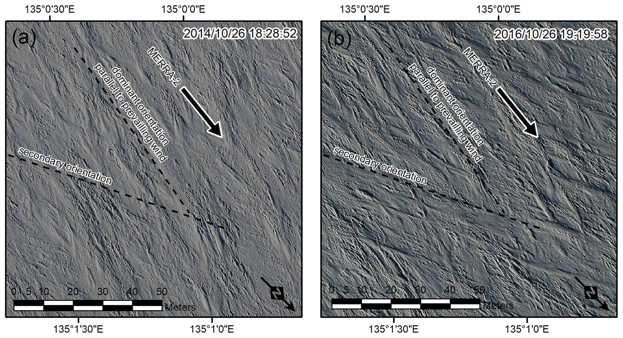
Figure 2DMS natural color images of the same area at 88∘ S and 135∘ E. The location is indicated in Fig. 3b. The two aerial images are nadir-looking, geolocated, and orthorectified color photographs of a sun-illuminated snow surface taken from 460 m a.g.l. The two photographs were taken on the same day of year 2 years apart. The low-angle sun illuminates the elongated, elevated surface features (sastrugi) facing the sun and creates dark shadows in the opposite direction behind the elevated features. For the 2014 image the sun is 11.5∘ above the horizon (accounting for refraction through the atmosphere) and for the 2016 image it is 12.1∘. The orientations of sastrugi, indicated by dashed lines, are determined by visually following transitions of elongated bright, sun-illuminated features and corresponding shadows. Both images show a dominant sastrugi orientation parallel to the 26-year averaged 10 m wind field from MERRA-2 (e.g., Gelaro et al., 2017) and a secondary orientation that appears to be less pronounced in 2014 compared to 2016.
2.4 Survey flights
Between 2014 and 2017 six NASA OIB airborne geophysical survey flights were completed to acquire data around 88∘ S (Table 1). Two flights are necessary to complete the entire small circle around 88∘ S with the platforms and bases of operations used. Snow and Ku-band radar data and DMS images are only available for 2014 and 2016 years. The combination of simultaneous laser altimetry, snow radar stratigraphy, and natural color imagery on a regional scale provides a unique data set to study small-scale deposition and erosional processes and their temporal and spatial variability.
Table 1Science instruments and airborne platforms of six NASA OIB aerogeophysical survey flights at 88∘ S.

n/a: not applicable.
3.1 Background
The surface roughness of polar ice sheets is primarily a result of ice dynamics and surface–atmosphere interactions on varying temporal and spatial scales. In general, ice flow over rugged bedrock topography causes roughness features that can extend from several hundreds of kilometers to a few kilometers depending on ice thickness, flow speed, and basal conditions (e.g., Smith et al., 2006, and references therein). These large-scale variations in ice surface topography caused by ice dynamics are not the topic of this analysis. Here, we focus on small-scale surface roughness or surface texture that spans from several meters to hundreds of meters and is primarily the result of ice–atmosphere interactions, such as wind deposition and wind-induced ablation or erosion, the predominant types of surface–atmosphere interactions in the area of 88∘ S. Sastrugi are the dominant form of small-scale surface roughness in the interior of polar ice sheets and are known to form parallel to the prevailing wind direction. Their orientation can therefore be used to infer time-averaged prevailing wind directions (e.g., Bromwich et al., 1990; Gow, 1965). Lister and Pratt (1959) describe sastrugi on the order of 20–30 m along the route of the Commonwealth Trans-Antarctic Expedition that also crossed 88∘ S. Figure 2 shows natural color DMS images of the same area at 88∘ S and 135∘ E taken 2 years apart. The dominant sastrugi orientation matches the 26-year average (1980–2016) of the 10 m wind direction from MERRA-2 (Modern-Era Retrospective Analysis for Research and Applications; e.g., Gelaro et al., 2017) (Fig. 3a). The ice surface on the East Antarctic plateau often has a dominant sastrugi orientation with sometimes two or three populations of sastrugi forming a crossing network of ridges that reflects seasonal changes in wind orientation (e.g., Warren et al., 1998) (Fig. 2). These seasonal changes are not captured in our averaged MERRA-2 wind direction. The good agreement between the dominant sastrugi orientation and the MERRA-2 long-term average, however, suggests that a single dominant wind direction is a good representation of the conditions in the survey area (Fig. 2).

Figure 3(a) Ice surface elevation from CryoSat-2 (Helm et al., 2014a) and 26-year 10 m average wind speed from MERRA-2 (e.g., Gelaro et al., 2017). The red line marks the location of 88S∘ S airborne geophysical data collection. TD is Titan Dome. (b) Ice surface roughness from 2014 ATM data (Studinger, 2014, updated 2018). The background image is a MODIS mosaic of Antarctica 2013–2014 (Haran et al., 2014) using MODIS data between November 2013 and March 2014. Locations of megadune fields are marked in orange, and roughness features A, B, and C refer to Fig. 4b. The location of the segment with a smooth surface in 2016 and 2017 between 175∘ W and 60∘ E that is discussed in Sect. 3.4 and shown in Fig. 4 is marked by a green line.
In recent decades, especially in the rapidly warming West Antarctic region, synoptic heat- and moisture-bearing storms have reached the South Pole area (e.g., Harris, 1992; Nicolas and Bromwich, 2011). Such storms and cyclonic events have been less common, though they still occur in the interior of East Antarctica (e.g., Gorodetskaya et al., 2014; Hirasawa et al., 2000). Individual sastrugi can be eroded and reform during a single storm (Warren et al., 1998). Most changes, however, occur as a result of seasonal changes between summer and winter months (e.g., Gow, 1965). Gow (1965) shows that sastrugi form during winter months, resulting in a rough surface, and subsequently get eroded during the summer by sublimation and deflation at the South Pole. This effect mostly results in a flattening of the subsurface layer stratigraphy and therefore does not affect our surface roughness results.
3.2 Relevance of surface roughness and slope for altimetry and surface mass balance
The surface roughness and slope of ice sheets affect several processes that are relevant for ice sheet mass balance (e.g., Gow, 1965, and references therein; van der Veen et al., 2009). King et al. (2004) describe small-scale variations in accumulation rate on the order of 1 km that appear to be associated with wind-borne redistribution as a function of slope. Hamilton (2004) found significant variability in snow accumulation rates due to the interaction of prevailing winds with meter-scale surface topography, where, for example, a concave depression can receive up to 18 % more accumulation than adjacent steeper snow surface topography. Similarly, Arcone et al. (2012) mapped accumulation patterns in East Antarctica that are created by wind-blown deposition on windward and leeward slopes. Slope-dependent accumulation is also related to spatial variations in firn density (Grima et al., 2014), which impacts mass balance estimates from altimetry data. Small-scale roughness contributes to noise in firn core records and therefore accumulation rate estimates (van der Veen et al., 1998, 2009). Studies by van der Veen et al. (1998, 2009) used ATM roughness estimates over Greenland to determine the uncertainty in water equivalent (w.e.) accumulation estimates from shallow firn cores.
Surface roughness also affects the albedo and bidirectional reflectance distribution function of ice sheets (Leroux and Fily, 1998; Warren et al., 1998). Nolin et al. (2002) used ATM roughness estimates to calibrate Multi-angle Imaging SpectroRadiometer (MISR) roughness estimates, and Nolin and Payne (2007) then derived relationships between ice surface roughness and near-infrared albedo using ATM and MISR data. Ongoing satellite and modeling investigations on radiative impacts of surface roughness and sastrugi continue to illuminate angular relationships and parameterizations that can be key to quantifying bidirectional reflectance distribution function and albedo sensitivities in ice surface studies (e.g., Corbett and Su, 2015; Kokhanovsky and Zege, 2004; Larue et al., 2020). As ice sheet surface roughness mapping and modeling capabilities improve, it will be possible to more accurately include the radiative effects of surface roughness. Surface roughness furthermore affects thermodynamic fluxes because it affects boundary layer processes through the aerodynamic roughness and therefore the surface energy balance (Boisvert et al., 2017; Chambers et al., 2019; Nolin and Mar, 2018; Palm et al., 2017).
3.3 Surface roughness estimates – methods
There are several diverse approaches to quantifying topographic irregularity or surface roughness (e.g., Smith, 2014, and references therein). In general, roughness metrics are not only scale, and orientation-dependent, but also impacted by the spatial resolution, footprint size, and sample spacing of the input data. One commonly used metric for surface roughness is the standard deviation σ of small-scale elevation fluctuations from a mean or de-trended surface in a given area or over a given length (e.g., Das et al., 2013; Smith, 2014, and references therein). In order to minimize potential effects from anisotropy in surface roughness over different length scales and orientations, we have calculated surface roughness over an area roughly square in size common to both laser altimeters. Individual spot elevation measurements are binned into 0.06∘ longitude segments (240 m in length at 88∘ S). We then fit a third-order polynomial regression model through all spot elevation measurements within a longitude segment. We define the standard deviation σ of the residuals as a metric for surface roughness.
For estimation of surface roughness from snow radar data, we pick an initial surface for each radar trace record (every ∼5 m along track) by finding the maximum slope in the radar return power across nine discrete time intervals called range bins. The size of a range bin in firn with a density of 550 kg m−3 is 1.8 cm. Starting at the initial surface pick, we keep sliding the surface pick one range bin deeper (or later in time) while the slope for the range bin remains above 3 standard deviations of the mean, which provides our final surface. Next, surface picks that lie outside of a 15-range bin window from a smoothed surface are discarded and set to the smoothed surface; however, very few data points are discarded (1.8 %). Surface roughness is estimated from residuals to the smoothed surface fit. Specifically, surface roughness for a given location is calculated as the standard deviation in surface range-bin residuals for locations within a 250 m radius. This radius was selected to ensure consistency with laser-altimeter-derived roughness values. Finally, the range-bin roughness is converted to heights by using the radar wave velocity in air (2.998×10⁸ m s−1).
For a closer look at very fine-scale spatial and temporal changes in surface roughness around 88∘ S, we use roughness estimates contained in the ATM Level 2 smoothed ice surface data product, known as ICESSN. The ICESSN data product includes slope and roughness estimates in overlapping 80 m×80 m platelets across the swath (Studinger, 2014, updated 2018). The root mean square of the residuals of a plane fit through the platelets is an estimate of the surface roughness. Removing the mean results in the root mean square being equivalent to the standard deviation σ.
Figure 4 shows the surface roughness estimates around 88∘ S latitude from three different instruments and over the course of 3 different years. In general, there is good agreement between the roughness estimated using the ATM laser altimeter and the synchronous roughness estimates from the snow radar (Fig. 4b, c). Because of the smaller footprint size and higher sampling density, the ATM laser-derived roughness estimates are slightly larger than the radar estimates, with few exceptions. The radar estimates also reveal more scatter, probably caused by the much lower range resolution of the radar compared to the ATM laser altimeter. The mean difference of the laser minus snow radar roughness estimates is 0.6±1.9 cm for 2014 and 1.6±2.1 cm for 2016; however, the spatial patterns, which are of main interest for this study, are nearly indistinguishable. There are no obvious spatial patterns in the roughness difference between laser and radar that would reflect a geophysical signal. Because of the higher point density, roughness derived from the UAF Riegl system is larger than the ATM roughness estimates. The mean difference between the 2017 UAF minus 2016 ATM laser estimates is 1.2±2.4 cm.
A 370 km long segment between 150∘ W and 100∘ E was repeated in 2017 within 3 d with the same instrument. It is unlikely that the surface was significantly altered within 3 d, and therefore the difference between the two estimates can be used as an approximate estimate of the instrument-specific accuracy and precision of the laser-derived roughness estimates. The mean surface roughness for the first east-bound flight is 9.5±1.5 and 10.1±2.0 cm for the later west-bound flight. The mean μ of the difference in surface roughness between the two 2017 flights is 0.02 cm with a σ of 0.7 cm. For comparison, a separate study by Das et al. (2013) over Dome Argus with a Riegl LMS–Q240i scanner shows a similar range of roughness as our measurements around 88∘ S.
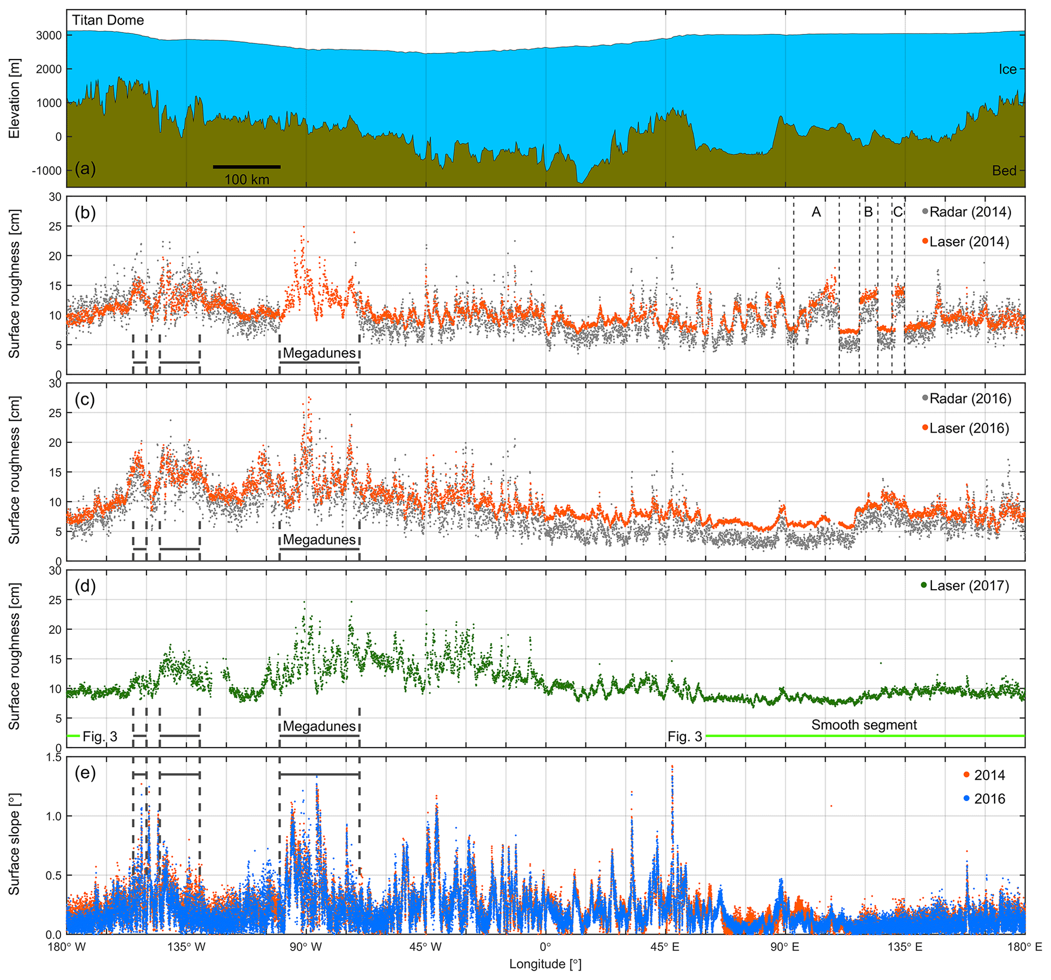
Figure 4(a) Ice surface elevation from 2014 ATM data (Studinger, 2014, updated 2018) and bedrock topography from 2014 CReSIS Multichannel Coherent Radar Depth Sounder (MCoRDS) data (Leuschen et al., 2010, updated 2018). The profile starts at Titan Dome (TD) and moves clockwise around 88∘ S. (b) Surface roughness from 2014 ATM laser and snow radar data. A 14 min disk failure of the snow radar in 2014 resulted in a data gap over the megadunes. (c) Same for 2016. (d) Surface roughness from 2017 UAF laser data. The location of the smooth segment between 175∘ W and 60∘ E that is discussed in Sect. 3.4 and also shown in Fig. 3b is indicated by a green line. (e) Surface slope from 2014 and 2016 ATM ICESSN data using only the nadir platelet (Studinger, 2014, updated 2018). Heavy dashed lines in (b)–(e) mark megadune areas, and thin dashed lines in (b) indicate distinct abrupt changes in surface roughness in 2014.
3.4 Surface roughness, slope, and elevation around 88∘ S – results
In order to distinguish ice surface roughness features caused by ice dynamics from roughness features that are a result of ice–atmosphere interactions, the proximity of the ice surface to bedrock topography and bedrock roughness must be understood (Fig. 4a). The large ice thickness (Fig. 4) and slow ice flow velocities (<10 m yr−1; Mouginot et al., 2019) in the survey area, combined with the small window size we use to calculate the roughness make it unlikely that any of the roughness features we observe are ice dynamic related. Thus, we interpret the roughness characteristics shown in Figs. 3 and 4 as caused by ice–atmosphere interactions.
Figures 3b and 4 show several spatially coherent segments with distinct roughness characteristics around 88∘ S that appear not to be related to ice dynamics. In general, the surface roughness estimated from snow radar and laser altimetry data varies between 2 and 25 cm. The smoothest surface in 2016 and 2017 is between 175∘ W and 60∘ E and includes Titan Dome. The location of this segment is indicated by green lines in Figs. 3b and 4d. The smooth segment also coincides with the highest ice surface elevations and shallowest surface slopes around 88∘ S (Fig. 4).
The segment between 70 and 100∘ W shows a pronounced increase in roughness in 2014 (Fig. 4b). The MODIS Mosaic of Antarctica (MOA; Haran et al., 2014) shows that this segment is near the edge of a megadune field that is mostly north of 88∘ S (Fig. 3b). Megadunes are long-wavelength surface ripples (Fahnestock et al., 2000) with amplitudes on the order of a few meters (peak to trough) and wavelengths of several kilometers (Fahnestock et al., 2000; Scambos and Fahnestock, 1998). The typical elevation pattern of megadunes is not visible in the 88∘ S laser altimetry data. The likely reasons for this are that the airborne geophysical data were collected at the edge of the dune field, and the orientation of the dune crests is subparallel to the airborne geophysical data. The orientation of dune crests between 70 and 100∘ W is approximately perpendicular to the prevailing surface wind direction from MERRA-2 (Fig. 3a) consistent with findings from Fahnestock et al. (2000).
A second megadune field can be seen between 130–145 and 150–155∘ W (Figs. 3 and 4). The surface of this dune field is less rough in 2017 compared to 2014 and 2016. Data for MOA were collected between November 2013 and March 2014. The temporal stability of megadune fields remains poorly understood. Fahnestock et al. (2000) found 60 m of dune migration over a 34-year period for a megadune field in the vicinity of Vostok Station, approximately 1100 km from the dune field discussed here. Therefore dune migration rates could vary significantly between the two sites. Since our survey area is near the edge of the dune field, we cannot rule out that over the course of 4 years the edge of the dune field has migrated out of the coverage of the airborne geophysical data.
The slope of the ATM ICESSN nadir platelets shows many distinct peaks that are aligned very well between the 2014 and 2016 data, indicating that these features are stable in location (Fig. 4e). The mean μ and standard deviation σ of the surface slope around 88∘ S are 0.20∘ ± 0.16∘ and never exceed 1.5∘.
3.5 Temporal changes in surface roughness – results
We use ATM Level 2 ICESSN roughness estimates for a closer look at multiyear temporal changes in surface roughness around 88∘ S (Fig. 5) because they are calculated over 80 m×80 m platelets. The 2014 data reveal several areas where surface roughness doubles over very short spatial scales of only a few hundred meters (Fig. 4a). These features, labeled A, B, and C in Fig. 4b, are several tens of kilometers wide and appear to be oriented parallel to the main sastrugi direction visible in simultaneously collected ATM spot elevation data and Digital Mapping System (DMS) imagery. Figure 5 shows a close-up of one of the features (C). The rougher surface features are also present in the simultaneously collected CReSIS snow radar data (Fig. 5a, c).
These areas of increased surface roughness disappear in 2016 or seem to be significantly reduced in amplitude with the sharpness of the edges significantly blurred. Both the laser-derived surface roughness and the roughness estimated from snow radar data seem to be slightly lower than the smooth area. In 2017, the segments labeled A, B, and C appear to have no distinct roughness anomaly (Fig. 4d) compared to the surrounding areas.
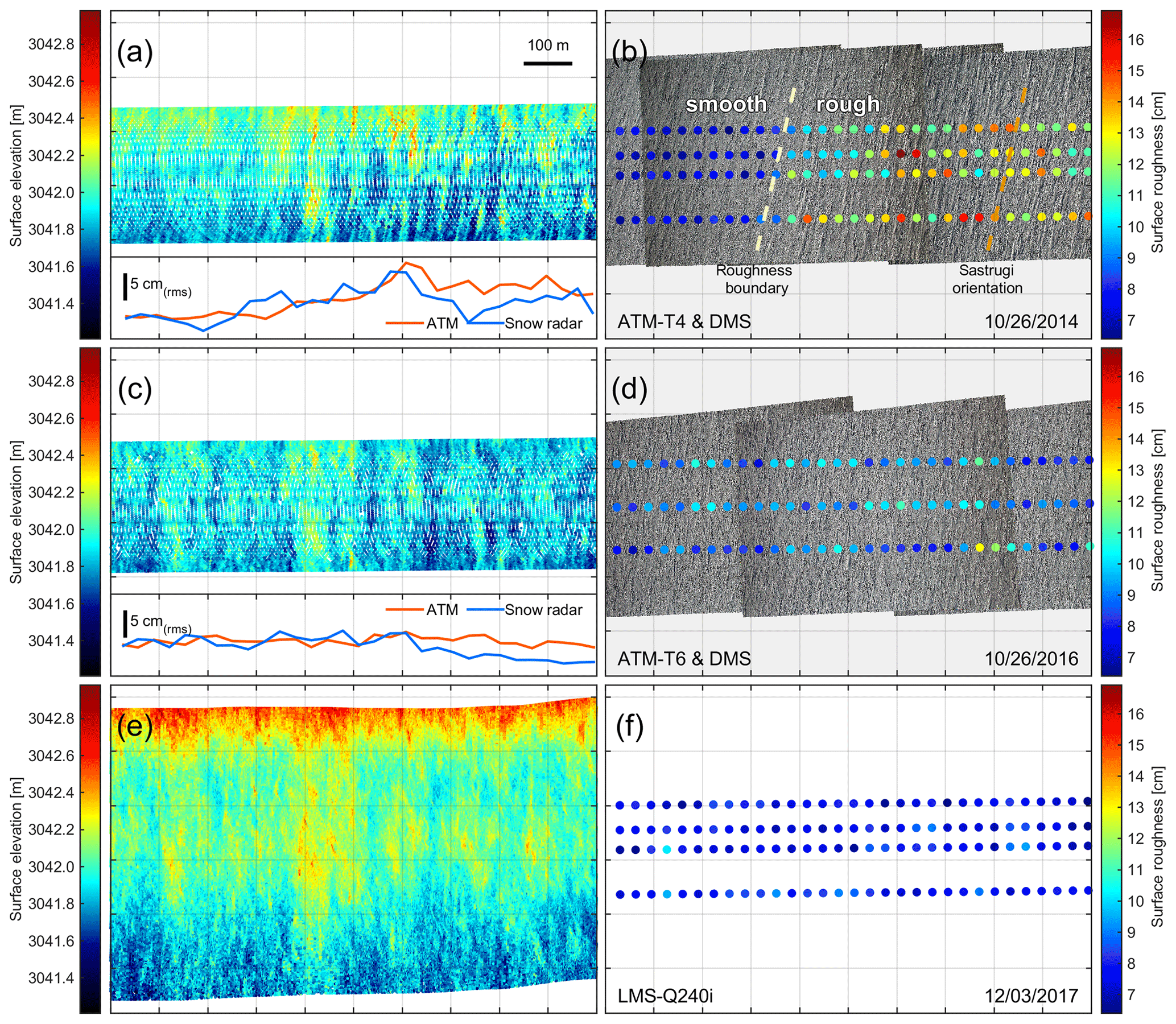
Figure 5Laser spot elevation measurements and DMS imagery over roughness feature “C” (Fig. 4b). The center of all map panels is at 88.97∘ S, 135∘ E. All panels cover the exact same area on the ground and are shown in a local coordinate system parallel to the aircraft trajectory. Panels (a), (c), and (e) show laser spot elevation measurements in 2014, 2016, and 2017. Inset plots in (a) and (c) show surface roughness from ATM and snow radar at the center of the scan/nadir position. Panels (a) and (c) show small (centimeter level) semicircular elevation biases that are a result of occasional variations in scan azimuth speed (Yi et al., 2015). The peak-to-peak amplitude of these biases is an order of magnitude smaller than the ice surface topography. Panels (b), (d), and (f) show corresponding DMS imagery (b and d only) and surface roughness from laser altimetry in 2014, 2016, and 2017. The darkening towards the edge of the DMS frames in (b) and (d) is caused by vignetting from the lens and not related to geophysical changes. ATM roughness is from ICESSN data, and the UAF Riegl data from 2017 have been calculated in the same way as ATM ICESSN data to make them compatible. A distinct change in roughness can be seen in 2014 that is visible in both the laser-derived surface roughness and the length of the shadows in DMS imagery (b). The roughness doubles over a distance of ∼200 m (a). The orientation of the boundary is parallel to the dominant sastrugi orientation (b). In 2016 and 2017 the distinct change in roughness seems to have been smoothened out.
For snow-radar-derived accumulation calculations, we first stack traces to an approximate along-track separation of 100 m (∼18 traces), which largely reduces noise in the return power, especially at depth. These stacked echograms are then combined into segments of ∼100 km. A single radar reflection horizon, assumed isochronous, is tracked through the 100 km segment. The actual horizon picked will likely vary from segment to segment because we chose to map the strongest and most continuous reflection within that segment. The horizon is picked semiautomatically. First, the user visually selects the horizon of interest. The range bin with the strongest return power within a 15-bin window is then selected as the horizon “pick” for that trace. That pick is extended laterally across all traces by finding the strongest return power in adjacent traces within the 15-bin window. The user can then modify the picks if they deviate from their visual interpretation. The user can also eliminate portions of a given horizon if visual inspection deems horizon differentiation impossible. The spatial variability in accumulation rates and the varying strength of signal return prevent the calculation of temporally consistent accumulation rate from a single continuous horizon around the entirety of 88∘ S. Thus, the accumulation rates estimated for each 100 km segment will span differing time intervals; however, because of the relatively low accumulation rates, the majority span several decades, minimizing the impact of interannual variability.
For each 100 km segment, we estimate the spatial variability in snow accumulation using the aforementioned horizon picks. Typically, radar-derived accumulation rates rely on knowledge of the horizon age as well (e.g., Medley et al., 2013, 2014), but a lack of nearby dated ice core stratigraphy or clearly defined annual horizons restricts our ability to assign an age to our horizon picks. Because our work is focused on evaluating the spatial variability in snow accumulation, we develop a method that approximates the age of a given horizon through combination of horizon depths and MERRA-2 mean annual precipitation minus evaporation (P−E). In such a manner, our large-scale mean accumulation rates are forced to large-scale MERRA-2 P−E; however, rates are allowed to vary on <1 km length scales from our radar horizon picks. We detail the methodology below.
Assuming each horizon pick within a given segment is isochronous, we need to determine a way to approximate the age of that horizon. To do so, we begin by determining the mean accumulation rate and 2 m air temperature from MERRA-2 over the entire segment and use those variables to model steady-state firn density and age profiles using Herron and Langway (1980). The two-way travel time (τ) between the surface and the horizon pick is converted into depth (d) assuming
where c is the speed of light and ε is the integrated dielectric permittivity of the material above the horizon and x is the distance along the flight line. Specifically, we use the modeled depth–density profile to generate depth-dielectric permittivity based on Kovacs et al. (1995), which is then used to relate depth and two-way travel time with a depth-varying radar-wave velocity. Using this model, we interpolate horizon two-way travel time to depth. Depths vary along track (as our layer pick varies), but our large-scale depth–age model from Herron and Langway (1980) does not; thus, we will estimate a variable along-track age of the radar horizon. The use of a single firn density model for the entire 88∘ S circle is justified because the difference between the minimum and maximum accumulation rates is relatively small. The along-track variability is counter to our initial assumption that the radar horizons are isochronous; however, when we take the average age along track, we effectively force the overall mean accumulation rate for the segment to the large-scale MERRA-2 mean. We then use this age to calculate spatially varying accumulation rates along the entire segment as outlined by Medley et al. (2015). In such a manner, we force the large-scale mean accumulation rates to those prescribed by MERRA-2 but allow for small-scale variability derived from the snow radar horizon picks in the absence of independent estimates of firn depth–age profiles (Dattler et al., 2019). For comparison we have plotted all existing accumulation measurements of Favier et al. (2013) in Fig. 6c over our MERRA-2 and radar-derived accumulation rates. These snow pit measurements include data from the 1962–1963 South Pole Traverse (Taylor, 1971). While there is general agreement, it should be pointed out that Favier et al. (2013) applied the quality rating of Magand et al. (2007), which identifies all snow pit data points shown in Fig. 6c as low quality and subsequently excludes these data points from the quality-controlled version presented in Favier et al. (2013). Further limitations of the comparison are the long time between the snow pit measurements and airborne data and the large variability in snow accumulation rates on length scales of 10 km that can be seen in the radar-derived snow accumulation rates.
Previous work used the mean slope in the mean wind direction (MSWD) for studying relationships between surface slope and spatial variability in snow accumulation rates (e.g., Das et al., 2013; Dattler et al., 2019; Scambos et al., 2012). MSWD is defined as the scalar dot product between the surface slope with the mean wind direction (Scambos et al., 2012). Here, we use the time-averaged zonal and meridional wind components u and v from MERRA-2, transformed in to a Cartesian polar-stereographic projection, to calculate the mean wind direction. Analyzing relationships between surface slope, accumulation rates, and mean wind direction at 88∘ S is limited by the latitudinal resolution of the MERRA-2 reanalysis model, which is 0.5∘ or 55 km, as well as the cross-sectional nature of the geophysical surveys (i.e., the data represent a two-dimensional cross section). Given the narrow swath width of the ATM laser data (240 m), we use the ice surface slope derived from the CryoSat-2 DEM (Helm et al., 2014a) at 1 km resolution to calculate the MSWD. The slope south of 88∘ S is only weakly constrained due to the absence of elevation data imposing further limitations on the analysis. The MERRA-2 26-year 10 m wind field is interpolated to the CryoSat-2 DEM grid cell locations. The difference in spatial resolution between the surface DEM and MERRA-2 will result in MSWD uncertainty from oversampling the wind field. Because of the small slopes in the study area, however, we do not anticipate complex wind fields where actual wind orientation would significantly deviate from the MERRA-2 reanalysis model. Small topographic features, however, are not represented by the 10 m surface wind field as will be discussed later.
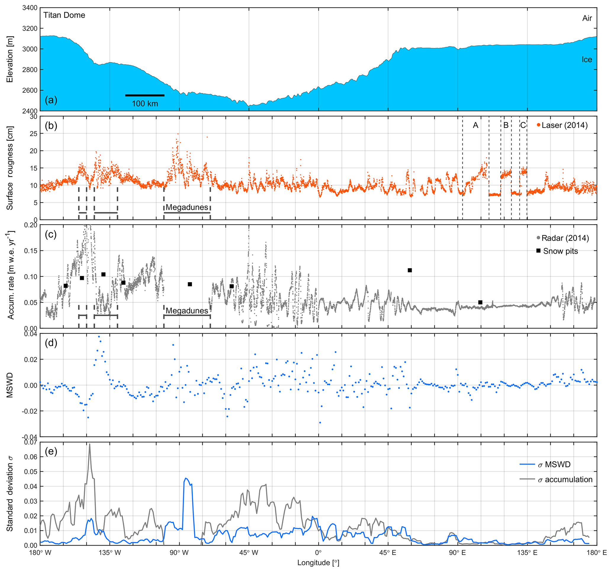
Figure 6(a) Ice surface elevation around 88∘ S from ATM laser altimetry. (b) Surface roughness from ATM laser altimetry. (c) Snow accumulation rate derived from 2014 snow radar data and tied to MERRA-2. A 14 min disk failure of the snow and Ku-band radars in 2014 resulted in a data gap over the megadunes and therefore the accumulation rate. Squares indicate accumulation measurements from snow pit data within 10 km of 88∘ S (Favier et al., 2013; Taylor, 1971). (d) Mean slope in the mean wind direction (MSWD) in 1∘ longitude bins (4 km). (e) Standard deviation σ of the MSWD and snow accumulation rate estimated over 20 km long segments.
In general, annual snow accumulation is around 5 cm w.e. yr−1 and is highest near the backside of the Transantarctic Mountains near 150∘ W, a region that is influenced by precipitation from cyclonic events penetrating the area from the Bellingshausen Sea and Ross Sea sectors (Casey et al., 2014; Nicolas and Bromwich, 2011) (Fig. 6). The highest accumulation rates (up to 20 cm w.e. yr−1) near 150∘ W coincide with a megadune field (Fig. 3b) and appear to be in a local topographic low at the flank of Titan Dome that trends perpendicular to the aerogeophysical survey profile around 88∘ S (Figs. 6a and A1a). The surface depression coincides with a 1000 m deep and 25 km wide bedrock low perpendicular to the profile (Studinger et al., 2006, and Fig. 3a). The dominant wind direction is near perpendicular to the survey profile and follows the trend of the ice surface low (Fig. 3a). The high-accumulation area also shows high surface roughness combined with steep slopes (Figs. 4 and A1). Another area with relatively high snow accumulation rates is located between 45∘ W and 0∘ longitude and is also exposed to precipitation from the Weddell Sea sector (e.g., Casey et al., 2014).
The snow accumulation rate at 88∘ S is spatially highly variable over very short length scales of several kilometers (Fig. 6c). Based on visual inspection small-scale variability in snow accumulation rate correlates with small-scale variability in ice surface elevation (Fig. 6a), suggesting that wind-driven erosion and deposition is a primary process of snow accumulation. The relatively constant surface elevation between 60 and 150∘ E shows very little variation in snow accumulation. In contrast, the short-scale (<10 km) undulations in ice surface elevation between 75∘ W and 45∘ E correspond to a highly variable (0–20 cm w.e. yr−1) snow accumulation pattern with a similar length scale (Figs. 6a, c and A2). The dominant wind direction in the western segment is subparallel to the profile (Fig. A2). Here, several pronounced peaks in snow accumulation rate correspond to topographic depressions in ice surface elevation (grey dashed lines in Fig. A2), indicating windblown deposition of snow. The eastern part of the profile has a wind direction oblique or perpendicular to the profile. However, several peaks in snow accumulation rate still correlate with topographic depressions. Near 90∘ E the wind direction is parallel to the profile (Fig. 3). A pronounced peak in snow accumulation rate at 90∘ E correlates with a 20 m deep depression in surface topography that is several kilometers wide (Fig. A3). Accumulation decreases on the lee side of the topographic high at the western shoulder of the depression and increases towards the lowest part of the depression where it reaches its highest point (Fig. A3). The general correlation of highs in accumulation rate with lows in topography results in an overall negative correlation coefficient of between accumulation rate and MSWD (Fig. 7a). DMS natural color imagery and laser altimetry data typically shows two dominant wind directions (Fig. 2). Our MERRA-2 wind direction is an average over seasonal variations in wind speed and likely reflects a wind direction somewhere between the two dominant orientations of sastrugi. Since we have no knowledge of when a particular layer of snow has been deposited during a year, it is not possible to do a more detailed analysis.
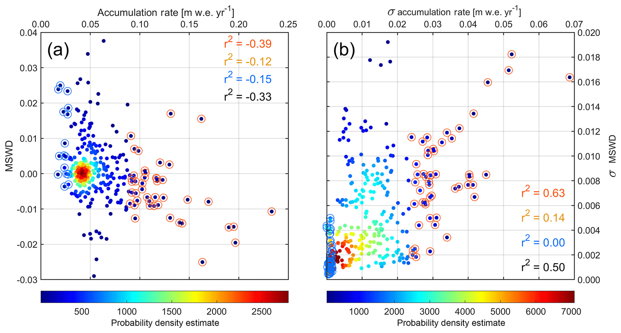
Figure 7(a) Mean slope in the mean wind direction (MSWD) versus snow accumulation rate around 88∘ S in 1∘ longitude bins (4 km). Since monochrome scatter plots can be misleading, we have used color coding to indicate regions with higher point density. Higher probability density estimates, calculated using a kernel estimate, are shown in warmer colors and indicate regions with higher point density. The probability density estimate is for visual clarity only and is not used for analysis or interpretation. Pearson's correlation coefficient for the entire data set. (b) Same for the standard deviation σ of the MSWD and snow accumulation rate with r2=0.50. σ is estimated over 20 km long moving windows. Data points below μ−σ are indicated with blue circles and r2 values are listed in blue. The upper subset consists of data points above μ+σ and is marked by red circles and red r2 values. The remaining data points fall within ±σ from μ, with r2 shown in orange (data points are not marked for clarity).
The surface roughness derived from ATM laser altimetry reflects roughness on a scale of <250 m and does not reflect ice surface slope changes on length scales of several kilometers. However, the MSWD (Fig. 6d) shows the same pattern of high variability between 75∘ W and 45∘ E and fairly constant values between 60 and 150∘ E. To quantify the relationship between variability in surface slope, wind direction, and accumulation rates, we use the standard deviation σ of the MSWD and snow accumulation rate calculated over a 20 km long moving window (Fig. 6e). Figure 6e shows the standard deviation of the MSWD and accumulation rate. In general, higher σ in accumulation rate generally occurs in areas with higher σ in MSWD. The match is strongest near 90∘ E where wind orientation is parallel to the profile.
The correlation coefficient between the standard deviations of the accumulation rate and the MSWD is r2=0.50, indicating a stronger link between these variables than the actual parameters (Fig. 7b). The magnitude of the correlation coefficient, however, is dependent on the length scale used to calculate the standard deviation. Dattler et al. (2019) find a similar behavior between σ accumulation rate and σ MSWD. Visual inspection of Fig. 7 suggests that the relationship between accumulation rate and MSWD and the σ of accumulation rate and σ of MSWD is more pronounced for larger magnitudes of the variables. A kernel density estimate quantifies the probability density estimate of nearby points and allows visualization of the point density using a color scale for the data points (Fig. 7). We divide the data set into three subsets using the mean μ and σ: the lower end is defined by values below μ−σ, while the upper end is values above μ+σ. The remaining points that are within ±σ from μ form the center subset. We have calculated correlation coefficients r2 for all subsets. In general, the correlation is strongest for the upper subsets, while the lower subsets show weak correlation. This is different from the results of Dattler et al. (2019), who find that the lower end also shows a strong correlation. The upper tenth percentile of our data have an r2 of 0.85 similar to the results of Dattler et al. (2019). Most of the data of Dattler et al. (2019) are located over high-accumulation areas in West Antarctica. A possible explanation for the weak correlation could be the very low accumulation rates in our area, combined with very small slopes and low wind speed. Noise in the elevation data will have a stronger impact on MSWD calculation, and similarly, subtle changes in surface slope are likely below the resolution of MERRA-2, therefore resulting in a noisier and thus uncorrelated lower subset.
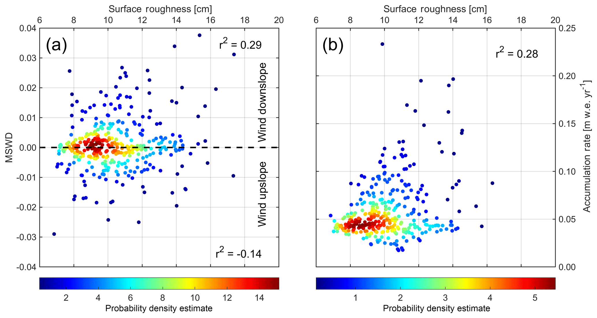
Figure 8(a) ATM-derived surface roughness versus mean slope in the mean wind direction (MSWD) around 88∘ S in 1∘ longitude bins (4 km). Color indicates the probability density estimate of nearby points using a kernel density estimate. Pearson's correlation coefficients r2 are calculated for upslope winds (MSWD<0) and downslope winds (MSWD>0). (b) Same for surface roughness versus accumulation rate.
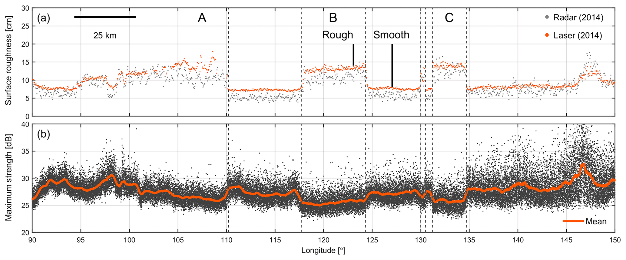
Figure 9(a) Surface roughness from 2014 ATM laser and CReSIS Ku-band radar data over roughness features “A”, “B”, and “C” (Fig. 4b). Vertical black lines mark the locations of radar waveforms over smooth and rough surfaces shown in Fig. A4. (b) Maximum of relative return signal strength from 2014 snow radar data. The red line is a running mean calculated over 350 radar traces (∼2 km), which is similar in size to the 1.65 km CryoSat-2 footprint in low-resolution mode (LRM) over smooth surfaces (Scagliola, 2013). The strength of the surface return is around 3 dB weaker over rough areas compared to smooth areas.
Wind-related deposition and ablation processes could cause spatial roughness variations depending on surface slope and wind direction. For example, windblown deposition of snow into concave surface depressions and ablation on upslope areas could create spatial surface roughness patterns that correlate with slope and wind direction. We use the MSWD to determine if slopes that are exposed to uphill winds have different surface roughness than slopes experiencing primarily downhill winds (Fig. 8a). We calculate r2 for upslope winds (MSWD<0) and downslope winds (MSWD>0). Neither the upslope winds () nor downslope winds (r2=0.29) show any statistically significant correlation between surface roughness and slope as can be seen in the scatter plot (Fig. 8a). Similarly, the surface roughness does not seem to be correlated with snow accumulation rates (r2=0.28), indicating that there is also no statistically significant slope-independent relationship between surface roughness and accumulation rates within our survey area (Fig. 8b). Correlations may exist in smaller local areas, but our data show that there is no consistent relationship between surface roughness, slope and wind direction on a regional scale within our survey area. However, our analysis is constrained by using two-dimensional high-resolution roughness estimates and correlating them with three-dimensional wind fields and surface slope with much lower spatial resolution.
Surface roughness impacts the return signal of radar altimeters and can therefore cause elevation biases (e.g.,van der Veen et al., 2009, and references herein) similar to slope-dependent errors in altimetry data (Helm et al., 2014a; Slater et al., 2018). Radar backscatter in radar altimeters such as CryoSat-2 is a function of surface roughness. Surface roughness at the length scales of the radar wavelength (2.2 cm) predominantly contributes to radar backscatter, which cannot be resolved by our laser data. Changes in surface roughness cause changes in radar backscatter through changes of the echo waveform, which can introduce range biases in the retrieval of surface elevation (Arthern et al., 2001; Kurtz et al., 2014). Figure 9 shows the maximum of the Ku-band radar return signal strength over the distinct roughness features identified from laser altimetry data (see Sect. 3.5). The maximum return energy over rougher surface areas is about 3 dB lower than over the smooth areas in between. The difference in return signal strength is even more pronounced for the snow radar (4 dB, not shown). Stacked Ku-band waveforms shown in Fig. A4 show 3 dB higher surface return power at 3.053 µs over a smooth surface compared to the rough surface. The amplitude of the subsurface backscatter below 3.06 µs, however, is similar in strength over smooth and rough areas (Fig. A4). This observation is consistent with the finding of Gow (1965) that heat from radiation causes crystal growth on the flanks of sastrugi, resulting in loosely bonded crystals that are prone to erosion by moderate winds (Gow, 1965). This differential sublimation–deflation-driven redistribution of snow flattens the surface topography at the end of the summer, resulting in relatively flat subsurface stratigraphy compared to the surface topography. The difference in waveform shapes between smooth and rough surfaces suggests that radar altimeters are potentially prone to elevation errors when threshold or leading edge trackers are being used for range retrieval. The Ku-band radar's relatively wide bandwidth and small footprint size allow resolution of the surface and subsurface layers and thus accurate tracking of the surface elevation. However, the reduced bandwidth and significantly larger footprint size of CryoSat-2 LRM returns does not allow for the resolution of individual layers, but instead leads to a pronounced broadening of the return waveform when the total cumulative backscatter of the sub-surface layers is close to, or exceeds, the backscatter from the surface layer.
The relatively small-scale nature and temporal variability of these features would require the use of more sophisticated retrieval techniques to better account for differences caused by the lower relative surface backscatter of rough areas. The elevation biases caused by temporal and spatial variability in surface roughness are in addition to elevation biases caused by wind-induced anisotropy in the firn that have been identified from crossover analysis (Armitage et al., 2014).
We have mapped the spatial and temporal variability in surface roughness and snow accumulation rate on a regional scale along a 1400 km circle around 88∘ S. We find significant small-scale variability (<10 km) in snow accumulation based on snow radar subsurface stratigraphy, indicating areas of strong wind redistribution are prevalent at 88∘ S. The observed small-scale variability in snow accumulation rates is not captured by existing reanalysis models such as MERRA-2, which have low spatial resolution. Our analysis shows that there is no simple relationship between surface slope, wind direction, and snow accumulation rates for the entire survey area. Previous studies have primarily focused on smaller regions, often showing good correlation between surface slope and accumulation rates, and are often used to falsely extrapolate parameters and relationships to larger regions beyond the study area. While we also observe these local correlations between surface slope, wind direction, and accumulation rates, our results show that even for a homogenous area like the East Antarctic plateau near the South Pole such simple relationships do not exist on a regional scale. At the same time, we note that our accumulation rate measurements are a simple two-dimensional view; until we have three-dimensional mapping of accumulation rates, these relationships might remain elusive. Our results underline the importance of regional-scale studies to derive accurate regional-scale parameterizations and relationships in light of expanding data sets, advances in high-performance computing, and sophistication in model development. Similarly, we find high variability in surface roughness derived from laser altimetry measurements on length scales smaller than 10 km, sometimes with very distinct and sharp transitions. These areas also show significant temporal variability over the course of the 3 survey years. We also find that surface roughness does not seem to be correlated with snow accumulation rates. There seems to be no statistically significant slope-independent relationship between surface roughness and accumulation rates within our survey area. The observed small-scale temporal and spatial variability in surface roughness will make it difficult to develop elevation bias corrections for radar altimeter retrieval algorithms.
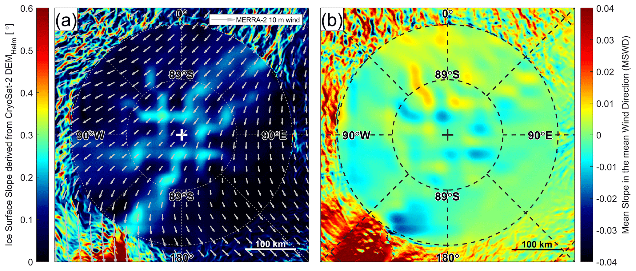
Figure A1(a) Ice surface slope in degrees derived from CryoSat-2 (Helm et al., 2014a) and 26-year 10 m wind average from MERRA-2 (e.g., Gelaro et al., 2017). (b) Mean slope in the mean wind direction (MSWD).
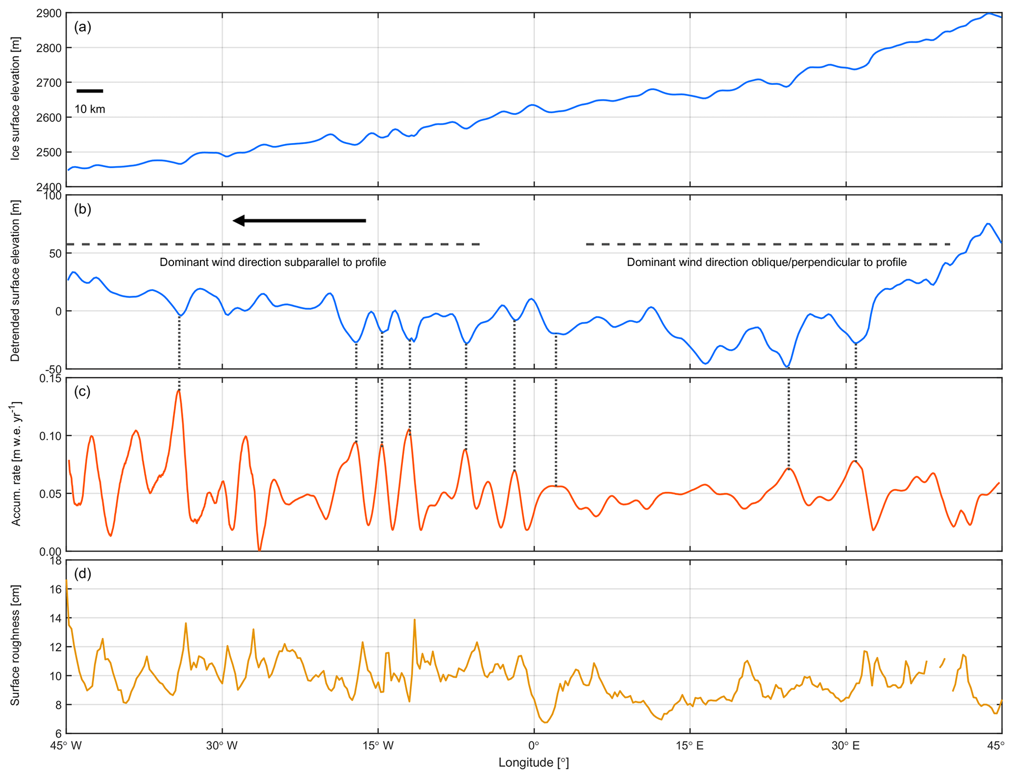
Figure A2(a) Ice surface elevation at 88∘ S between 45∘ W and 45∘ E from ATM laser altimetry. (b) Ice surface elevation with linear trend removed. (c) Snow accumulation rate. Several prominent peaks that spatially correlate with topographic depressions are marked by grey dashed lines. (d) ATM-derived ice surface roughness.
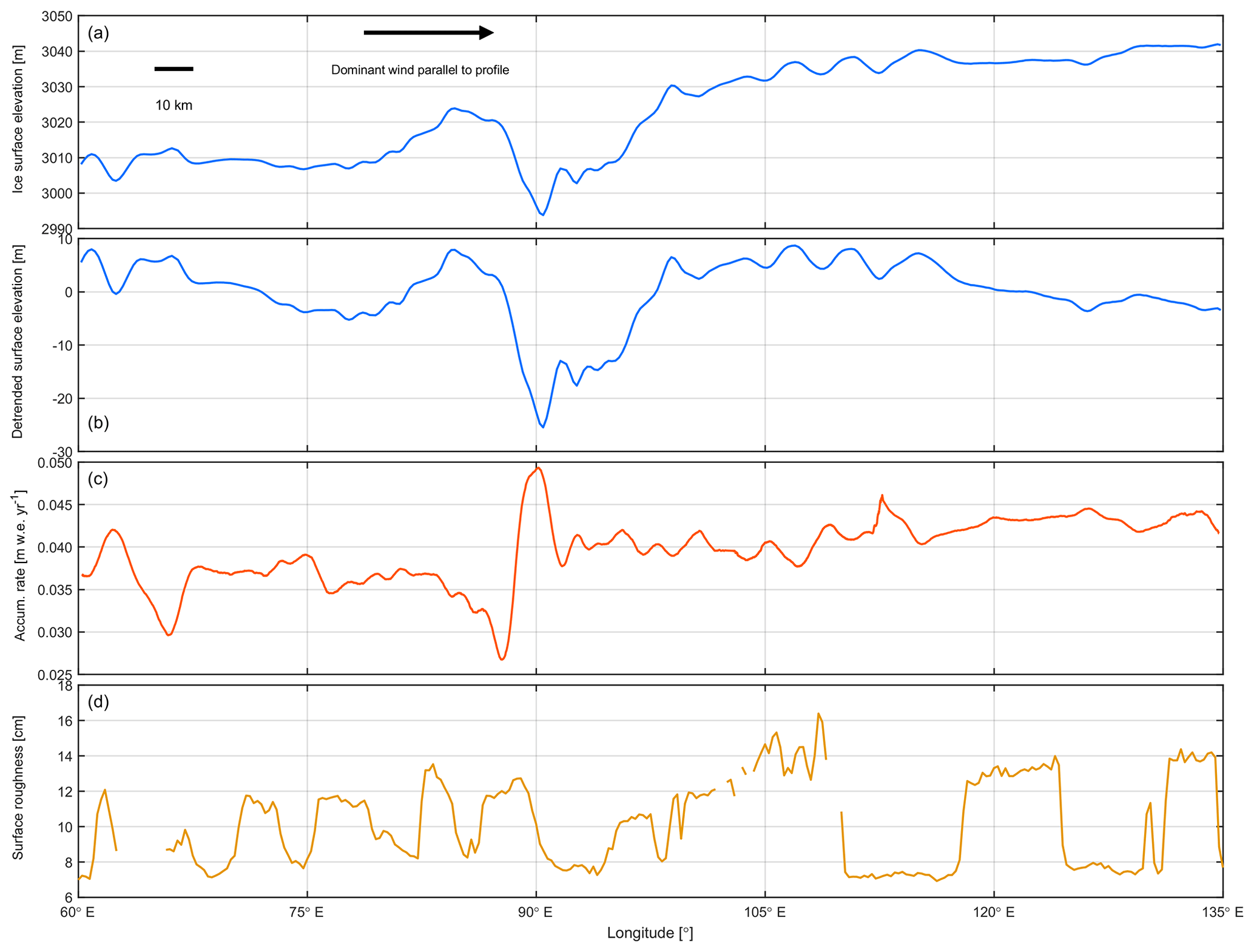
Figure A3(a) Ice surface elevation between 60 and 135∘ E from ATM laser altimetry. The dominant wind direction from MERRA-2 is parallel to the profile segment. (b) Ice surface elevation with linear trend removed. (c) Snow accumulation rate where the pronounced peak at 90∘ E corresponds to the topographic depression in the ice surface. (d) ATM-derived ice surface roughness.
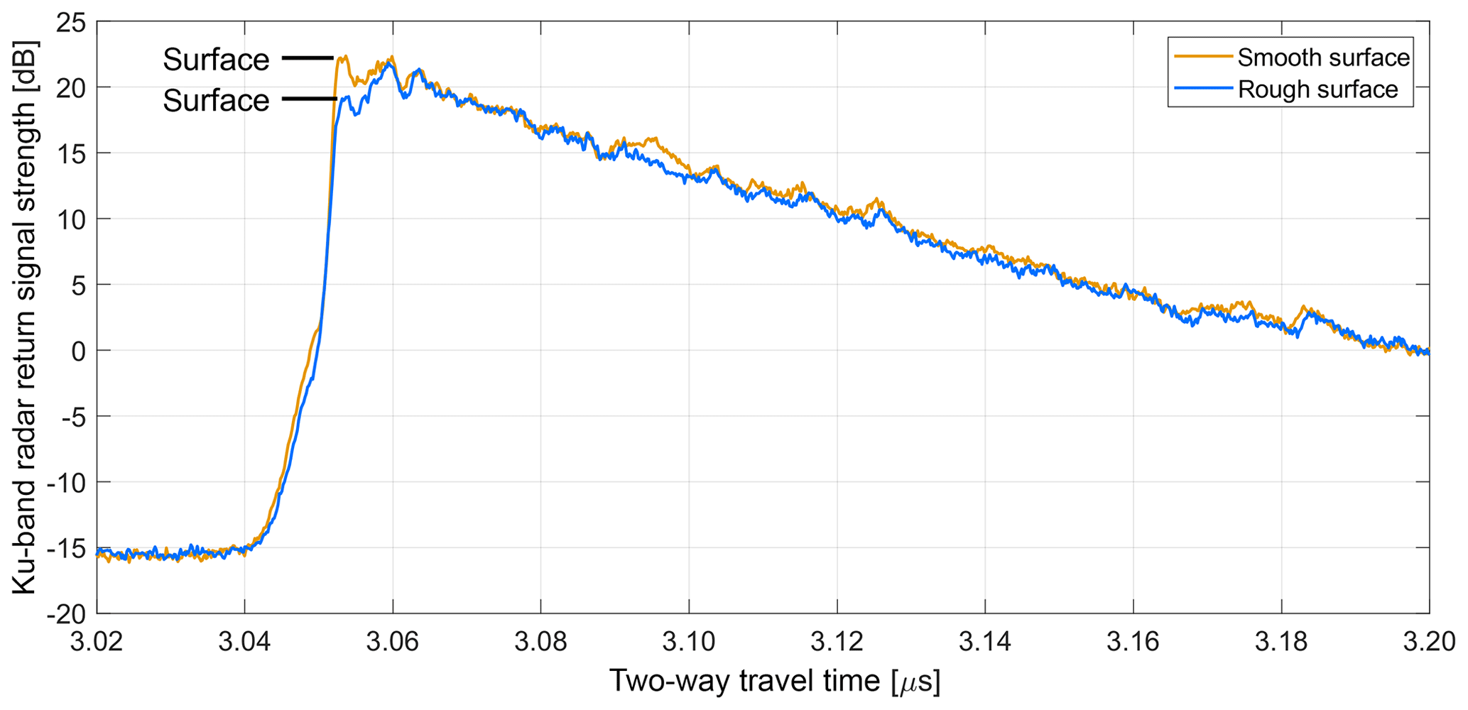
Figure A4Relative Ku-band radar return signal strength over smooth and rough surfaces. A total of 100 traces were stacked for the averaged waveforms. For location see Fig. 9. The difference between the radar waveforms indicates that radar altimeters are potentially prone to elevation errors when threshold or leading edge trackers are being used for range retrieval.
All NASA Operation IceBridge data used in this study are freely available at the National Snow and Ice Data Center (NSIDC, 2019) at https://nsidc.org/icebridge/portal (last access: 2019). The CryoSat-2 DEM from Helm et al. (2014a) is available at https://doi.org/10.1594/PANGAEA.831392 (Helm et al., 2014b). The MODIS Mosaic of Antarctica (MOA; Haran et al., 2014) is available from NSIDC at https://nsidc.org/data/nsidc-0730 (last access: 2019) (Haran et al., 208, updated 2019, https://doi.org/10.5067/RNF17BP824UM). MERRA-2 data are available at https://gmao.gsfc.nasa.gov/reanalysis/MERRA-2/data_access/ (last access: 2018). The Antarctic Digital Database is available at https://www.add.scar.org/ (last access: 2020).
MS led the analysis of the laser altimetry, optical imagery, and integration of results and prepared the manuscript with contributions from all co-authors. BCM derived surface roughness and accumulation rates from snow radar data and MERRA-2 and wrote the corresponding manuscript sections. KMB, KAC, and TAN contributed to the analysis and interpretation of surface roughness and accumulation rates. NTK and TBO contributed to the interpretation of radar backscatter and surface roughness. SSM contributed to the analysis and interpretation of the ATM laser altimetry data. All authors helped write the paper.
The authors declare that they have no conflict of interest.
We thank the Operation IceBridge instrument teams and flight crews for 11 years of data collection that made this study possible. Richard Cullather is thanked for discussions about MERRA-2. Mark Fahnestock is thanked for discussions about surface roughness, slope, and accumulation rates. We thank the reviewers Neil Ross and Joshua Chambers and the editor Nanna Bjørnholt Karlsson for constructive reviews that helped improve the manuscript.
This research has been supported by the NASA Cryospheric Sciences Program.
This paper was edited by Nanna Bjørnholt Karlsson and reviewed by Joshua Chambers and Neil Ross.
Abdalati, W., Zwally, H. J., Bindschadler, R., Csatho, B., Farrell, S. L., Fricker, H. A., Harding, D., Kwok, R., Lefsky, M., Markus, T., Marshak, A., Neumann, T., Palm, S., Schutz, B., Smith, B., Spinhirne, J., and Webb, C.: The ICESat-2 Laser Altimetry Mission, Proc. IEEE, 98, 735–751, https://doi.org/10.1109/jproc.2009.2034765, 2010.
Arcone, S. A., Jacobel, R., and Hamilton, G.: Unconformable stratigraphy in East Antarctica: Part I. Large firn cosets, recrystallized growth, and model evidence for intensified accumulation, J. Glaciol., 58, 240–252, https://doi.org/10.3189/2012JoJ11J044, 2012.
Armitage, T. W. K., Wingham, D. J., and Ridout, A. L.: Meteorological Origin of the Static Crossover Pattern Present in Low-Resolution-Mode CryoSat-2 Data Over Central Antarctica, Geosci. Remote Sens. Lett., IEEE, 11, 1295–1299, https://doi.org/10.1109/LGRS.2013.2292821, 2014.
Arthern, R. J., Wingham, D. J., and Ridout, A. L.: Controls on ERS altimeter measurements over ice sheets: Footprint-scale topography, backscatter fluctuations, and the dependence of microwave penetration depth on satellite orientation, J. Geophys. Res.-Atmos., 106, 33471–33484, https://doi.org/10.1029/2001jd000498, 2001.
Arthern, R. J., Winebrenner, D. P., and Vaughan, D. G.: Antarctic snow accumulation mapped using polarization of 4.3-cm wavelength microwave emission, J. Geophys. Res.-Atmos., 111, D06107, https://doi.org/10.1029/2004jd005667, 2006.
Boisvert, L. N., Lee, J. N., Lenaerts, J. T. M., Noël, B., Broeke, M. R., and Nolin, A. W.: Using remotely sensed data from AIRS to estimate the vapor flux on the Greenland ice sheet: Comparisons with observations and a regional climate model, J. Geophys. Res.-Atmos., 122, 202–229, https://doi.org/10.1002/2016JD025674, 2017.
Bromwich, D. H., Parish, T. R., and Zorman, C. A.: The confluence zone of the intense katabatic winds at Terra Nova Bay, Antarctica, as derived from airborne sastrugi surveys and mesoscale numerical modeling, J. Geophys. Res.-Atmos., 95, 5495–5509, https://doi.org/10.1029/JD095iD05p05495, 1990.
Brunt, K. M., Neumann, T. A., and Larsen, C. F.: Assessment of altimetry using ground-based GPS data from the 88S Traverse, Antarctica, in support of ICESat-2, The Cryosphere, 13, 579–590, https://doi.org/10.5194/tc-13-579-2019, 2019a.
Brunt, K. M., Neumann, T. A., and Smith, B. E.: Assessment of ICESat-2 Ice Sheet Surface Heights, Based on Comparisons Over the Interior of the Antarctic Ice Sheet, Geophys. Res. Lett., 46, 13072–13078, https://doi.org/10.1029/2019gl084886, 2019b.
Casey, K. A., Fudge, T. J., Neumann, T. A., Steig, E. J., Cavitte, M. G. P., and Blankenship, D. D.: The 1500 m South Pole ice core: recovering a 40 ka environmental record, Ann. Glaciol., 55, 137–146, https://doi.org/10.3189/2014AoG68A016, 2014.
Chambers, J. R., Smith, M. W., Quincey, D. J., Carrivick, J. L., Ross, A. N., and James, M. R.: Glacial aerodynamic roughness estimates: uncertainty, sensitivity and precision in field measurements, J. Geophys. Res.-Earth Surf., e2019JF005167, https://doi.org/10.1029/2019JF005167, 2019.
Corbett, J. and Su, W.: Accounting for the effects of sastrugi in the CERES clear-sky Antarctic shortwave angular distribution models, Atmos. Meas. Tech., 8, 3163–3175, https://doi.org/10.5194/amt-8-3163-2015, 2015.
Das, I., Bell, R. E., Scambos, T. A., Wolovick, M., Creyts, T. T., Studinger, M., Frearson, N., Nicolas, J. P., Lenaerts, J. T. M., and van den Broeke, M. R.: Influence of persistent wind scour on the surface mass balance of Antarctica, Nat. Geosci., 6, 367, https://doi.org/10.1038/ngeo1766, 2013.
Dattler, M. E., Lenaerts, J. T. M., and Medley, B.: Significant Spatial Variability in Radar-Derived West Antarctic Accumulation Linked to Surface Winds and Topography, Geophys. Res. Lett., 46, 13126–13134, https://doi.org/10.1029/2019gl085363, 2019.
Dominguez, R. T.: IceBridge DMS L1B Geolocated and Orthorectified Images, Version 1. [2014, 2016]: NASA National Snow and Ice Data Center Distributed Active Archive Center, https://doi.org/10.5067/OZ6VNOPMPRJ0, 2010, updated 2018.
Fahnestock, M. A., Scambos, T. A., Shuman, C. A., Athern, R. J., Winebrenner, D. P., and Kwok, R.: Snow megadune fields on the East Antarctic Plateau: extreme atmosphere-ice interaction, Geophys. Res. Lett., 27, 3719–3722, 2000.
Favier, V., Agosta, C., Parouty, S., Durand, G., Delaygue, G., Gallée, H., Drouet, A.-S., Trouvilliez, A., and Krinner, G.: An updated and quality controlled surface mass balance dataset for Antarctica, The Cryosphere, 7, 583–597, https://doi.org/10.5194/tc-7-583-2013, 2013.
Frezzotti, M., Urbini, S., Proposito, M., Scarchilli, C., and Gandolfi, S.: Spatial and temporal variability of surface mass balance near Talos Dome, East Antarctica, J. Geophys. Res.-Earth Surf., 112, F02032, https://doi.org/10.1029/2006jf000638, 2007.
Gelaro, R., McCarty, W., Suárez, M. J., Todling, R., Molod, A., Takacs, L., Randles, C. A., Darmenov, A., Bosilovich, M. G., Reichle, R., Wargan, K., Coy, L., Cullather, R., Draper, C., Akella, S., Buchard, V., Conaty, A., Silva, A. M. D., Gu, W., Kim, G.-K., Koster, R., Lucchesi, R., Merkova, D., Nielsen, J. E., Partyka, G., Pawson, S., Putman, W., Rienecker, M., Schubert, S. D., Sienkiewicz, M., and Zhao, B.: The Modern-Era Retrospective Analysis for Research and Applications, Version 2 (MERRA-2), J. Climate, 30, 5419–5454, https://doi.org/10.1175/jcli-d-16-0758.1, 2017.
Gomez-Garcia, D., Rodriguez-Morales, F., Leuschen, C., and Gogineni, S.: KU-Band radar altimeter for surface elevation measurements in polar regions using a wideband chirp generator with improved linearity, 2012 IEEE International Geoscience and Remote Sensing Symposium, 4617–4620, 2012.
Gorodetskaya, I. V., Tsukernik, M., Claes, K., Ralph, M. F., Neff, W. D., and Van Lipzig, N. P. M.: The role of atmospheric rivers in anomalous snow accumulation in East Antarctica, Geophys. Res. Lett., 41, 6199–6206, https://doi.org/10.1002/2014gl060881, 2014.
Gow, A. J.: On the Accumulation and Seasonal Stratification Of Snow at the South Pole, J. Glaciol., 5, 467–477, https://doi.org/10.3189/S002214300001844X, 1965.
Grima, C., Blankenship, D. D., Young, D. A., and Schroeder, D. M.: Surface slope control on firn density at Thwaites Glacier, West Antarctica: Results from airborne radar sounding, Geophys. Res. Lett., 41, 6787–6794, https://doi.org/10.1002/2014GL061635, 2014.
Hamilton, G. S.: Topographic control of regional accumulation rate variability at South Pole and implications for ice-core interpretation, Ann. Glaciol., 39, 214–218, https://doi.org/10.3189/172756404781814050, 2004.
Haran, T., Bohlander, J., Scambos, T. A., Painter, T. H., and Fahnestock, M. A.: MODIS Mosaic of Antarctica 2008–2009 (MOA2009) Image Map 2009: NASA National Snow and Ice Data Center Distributed Active Archive Center, https://doi.org/10.7265/N5KP8037, 2014.
Haran, T., Klinger, M., Bohlander, J., Fahnestock, M., Painter, T., and Scambos, T.: MEaSUREs MODIS Mosaic of Antarctica 2013–2014 (MOA2014) Image Map, Version 1, NASA National Snow and Ice Data Center Distributed Active Archive Center, Boulder, Colorado, USA, https://doi.org/10.5067/RNF17BP824UM, 2018, updated 2019.
Harpold, R., Yungel, J., Linkswiler, M., and Studinger, M.: Intra-scan intersection method for the determination of pointing biases of an airborne altimeter, Int. J. Remote Sens., 37, 648–668, https://doi.org/10.1080/01431161.2015.1137989, 2016.
Harris, J. M.: An analysis of 5-day midtropospheric flow patterns for the South Pole: 1985–1989, Tellus B, 44, 409–421, https://doi.org/10.1034/j.1600-0889.1992.00016.x, 1992.
Helm, V., Humbert, A., and Miller, H.: Elevation and elevation change of Greenland and Antarctica derived from CryoSat-2, The Cryosphere, 8, 1539–1559, https://doi.org/10.5194/tc-8-1539-2014, 2014a.
Helm, V., Humbert, A., and Miller, H/: Elevation Model of Antarctica derived from CryoSat-2 in the period 2011 to 2013, links to DEM and uncertainty map as GeoTIFF, PANGAEA, https://doi.org/10.1594/PANGAEA.831392, 2014b.
Herron, M. M. and Langway, C. C.: Firn Densification: An Empirical Model, J. Glaciol., 25, 373–385, https://doi.org/10.3189/S0022143000015239, 1980.
Hirasawa, N., Nakamura, H., and Yamanouchi, T.: Abrupt changes in meteorological conditions observed at an inland Antarctic Station in association with wintertime blocking, Geophys. Res. Lett., 27, 1911–1914, https://doi.org/10.1029/1999gl011039, 2000.
Johnson, A. J., Larsen, C. F., Murphy, N., Arendt, A. A., and Zirnheld, S. L.: Mass balance in the Glacier Bay area of Alaska, USA, and British Columbia, Canada, 1995–2011, using airborne laser altimetry, J. Glaciol., 59, 632–648, https://doi.org/10.3189/2013JoG12J101, 2013.
King, J. C., Anderson, P. S., Vaughan, D. G., Mann, G. W., Mobbs, S. D., and Vosper, S. B.: Wind-borne redistribution of snow across an Antarctic ice rise, J. Geophys. Res.-Atmos., 109, D11104, https://doi.org/10.1029/2003JD004361, 2004.
Kokhanovsky, A. A. and Zege, E. P.: Scattering optics of snow, Appl. Optics, 43, 1589–1602, https://doi.org/10.1364/AO.43.001589, 2004.
Kovacs, A., Gow, A. J., and Morey, R. M.: The in-situ dielectric constant of polar firn revisited, Cold Reg. Sci. Technol., 23, 245–256, https://doi.org/10.1016/0165-232X(94)00016-Q, 1995.
Krabill, W., Abdalati, W., Frederick, E., Manizade, S., Martin, C., Sonntag, J., Swift, R., Thomas, R., Wright, W., and Yungel, J.: Greenland ice sheet: High-elevation balance and peripheral thinning, Science, 289, 428–430, https://doi.org/10.1126/science.289.5478.428, 2000.
Krabill, W. B., Abdalati, W., Frederick, E. B., Manizade, S. S., Martin, C. F., Sonntag, J. G., Swift, R. N., Thomas, R. H., and Yungel, J. G.: Aircraft laser altimetry measurement of elevation changes of the greenland ice sheet: technique and accuracy assessment, J. Geodynam., 34, 357–376, https://doi.org/10.1016/s0264-3707(02)00040-6, 2002.
Kurtz, N. T., Galin, N., and Studinger, M.: An improved CryoSat-2 sea ice freeboard retrieval algorithm through the use of waveform fitting, The Cryosphere, 8, 1217–1237, https://doi.org/10.5194/tc-8-1217-2014, 2014.
Larsen, C. F.: IceBridge UAF Lidar Scanner L1B Geolocated Surface Elevation Triplets, Version 1. [2017], NASA National Snow and Ice Data Center Distributed Active Archive Center, https://doi.org/10.5067/AATE4JJ91EHC, 2010, updated 2018.
Larue, F., Picard, G., Arnaud, L., Ollivier, I., Delcourt, C., Lamare, M., Tuzet, F., Revuelto, J., and Dumont, M.: Snow albedo sensitivity to macroscopic surface roughness using a new ray-tracing model, The Cryosphere, 14, 1651–1672, https://doi.org/10.5194/tc-14-1651-2020, 2020.
Leroux, C. and Fily, M.: Modeling the effect of sastrugi on snow reflectance, J. Geophys. Res.-Planets, 103, 25779–25788, https://doi.org/10.1029/98JE00558, 1998.
Leuschen, C.: IceBridge Snow Radar L1B Geolocated Radar Echo Strength Profiles, Version 2. [2014, 2016], NASA National Snow and Ice Data Center Distributed Active Archive Center, https://doi.org/10.5067/FAZTWP500V70, 2014, updated 2018.
Leuschen, C., Gogineni, P., Rodriguez-Morales, F., Paden, J., and Allen, C.: IceBridge MCoRDS L2 Ice Thickness, Version 1: NASA National Snow and Ice Data Center Distributed Active Archive Center, https://doi.org/10.5067/GDQ0CUCVTE2Q, 2010, updated 2018.
Lister, H. and Pratt, G.: Geophysical Investigations of the Commonwealth Trans-Antarctic Expedition, The Geographical Journal published by The Royal Geographical Society (with the Institute of British Geographers), 125, 343–354, 1959.
Liu, H., Jezek, K., Li, B., and Zhao, Z.: Radarsat Antarctic Mapping Project Digital Elevation Model, Version 2, NASA National Snow and Ice Data Center Distributed Active Archive Center, https://doi.org/10.5067/8JKNEW6BFRVD, 2015.
Magand, O., Genthon, C., Fily, M., Krinner, G., Picard, G., Frezzotti, M., and Ekaykin, A. A.: An up-to-date quality-controlled surface mass balance data set for the 90∘–180∘ E Antarctica sector and 1950–2005 period, J. Geophys. Res.-Atmos., 112, D12106, https://doi.org/10.1029/2006jd007691, 2007.
Markus, T., Neumann, T., Martino, A., Abdalati, W., Brunt, K., Csatho, B., Farrell, S., Fricker, H., Gardner, A., Harding, D., Jasinski, M., Kwok, R., Magruder, L., Lubin, D., Luthcke, S., Morison, J., Nelson, R., Neuenschwander, A., Palm, S., Popescu, S., Shum, C. K., Schutz, B. E., Smith, B., Yang, Y., and Zwally, J.: The Ice, Cloud, and land Elevation Satellite-2 (ICESat-2): Science requirements, concept, and implementation, Remote Sens. Environ., 190, 260–273, https://doi.org/10.1016/j.rse.2016.12.029, 2017.
Martin, C. F., Krabill, W. B., Manizade, S. S., Russell, R. L., Sonntag, J. G., Swift, R. N., and Yungel, J. K.: Airborne Topographic Mapper Calibration Procedures and Accuracy Assessment, NASA Goddard Space Flight Center, Greenbelt, MD, report number NASA/TM-2012-215891, GSFC.TM.5893.2012, available at: https://ntrs.nasa.gov/citations/20120008479 (last access: September 2020), 2012.
McConnell, J. R., Bales, R. C., and Davis, D. R.: Recent intra-annual snow accumulation at South Pole: Implications for ice core interpretation, J. Geophys. Res.-Atmos., 102, 21947–21954, https://doi.org/10.1029/97jd00848, 1997.
Medley, B., Joughin, I., Das, S. B., Steig, E. J., Conway, H., Gogineni, S., Criscitiello, A. S., McConnell, J. R., Smith, B. E., van den Broeke, M. R., Lenaerts, J. T. M., Bromwich, D. H., and Nicolas, J. P.: Airborne-radar and ice-core observations of annual snow accumulation over Thwaites Glacier, West Antarctica confirm the spatiotemporal variability of global and regional atmospheric models, Geophys. Res. Lett., 40, 3649–3654, https://doi.org/10.1002/grl.50706, 2013.
Medley, B., Joughin, I., Smith, B. E., Das, S. B., Steig, E. J., Conway, H., Gogineni, S., Lewis, C., Criscitiello, A. S., McConnell, J. R., van den Broeke, M. R., Lenaerts, J. T. M., Bromwich, D. H., Nicolas, J. P., and Leuschen, C.: Constraining the recent mass balance of Pine Island and Thwaites glaciers, West Antarctica, with airborne observations of snow accumulation, The Cryosphere, 8, 1375–1392, https://doi.org/10.5194/tc-8-1375-2014, 2014.
Medley, B., Ligtenberg, S. R. M., Joughin, I., Van den Broeke, M. R., Gogineni, S., and Nowicki, S.: Antarctic firn compaction rates from repeat-track airborne radar data: I. Methods, Ann. Glaciol., 56, 155–166, https://doi.org/10.3189/2015AoG70A203, 2015.
Morlighem, M., Rignot, E., Binder, T., Blankenship, D., Drews, R., Eagles, G., Eisen, O., Ferraccioli, F., Forsberg, R., Fretwell, P., Goel, V., Greenbaum, J. S., Gudmundsson, H., Guo, J., Helm, V., Hofstede, C., Howat, I., Humbert, A., Jokat, W., Karlsson, N. B., Lee, W. S., Matsuoka, K., Millan, R., Mouginot, J., Paden, J., Pattyn, F., Roberts, J., Rosier, S., Ruppel, A., Seroussi, H., Smith, E. C., Steinhage, D., Sun, B., Broeke, M. R. V. D., Ommen, T. D. V., Wessem, M. V., and Young, D. A.: Deep glacial troughs and stabilizing ridges unveiled beneath the margins of the Antarctic ice sheet, Nat. Geosci., 13, 132–137, https://doi.org/10.1038/s41561-019-0510-8, 2020.
Mosley-Thompson, E., Paskievitch, J. F., Gow, A. J., and Thompson, L. G.: Late 20th Century increase in South Pole snow accumulation, J. Geophys. Res.-Atmos., 104, 3877–3886, https://doi.org/10.1029/1998jd200092, 1999.
Mouginot, J., Rignot, E., and Scheuchl, B.: Continent-Wide, Interferometric SAR Phase, Mapping of Antarctic Ice Velocity, Geophys. Res. Lett., 46, 9710–9718, https://doi.org/10.1029/2019gl083826, 2019.
Nicolas, J. P. and Bromwich, D. H.: Climate of West Antarctica and Influence of Marine Air Intrusions, J. Climate, 24, 49–67, https://doi.org/10.1175/2010jcli3522.1, 2011.
Nilsson, J., Gardner, A., Sandberg Sørensen, L., and Forsberg, R.: Improved retrieval of land ice topography from CryoSat-2 data and its impact for volume-change estimation of the Greenland Ice Sheet, The Cryosphere, 10, 2953–2969, https://doi.org/10.5194/tc-10-2953-2016, 2016.
Nolin, A. W. and Payne, M. C.: Classification of glacier zones in western Greenland using albedo and surface roughness from the Multi-angle Imaging SpectroRadiometer (MISR), Remote Sens. Environ., 107, 264–275, https://doi.org/10.1016/j.rse.2006.11.004, 2007.
Nolin, A. W., Fetterer, F. M., and Scambos, T. A.: Surface roughness characterizations of sea ice and ice sheets: case studies with MISR data, IEEE T. Geosci. Remote, 40, 1605–1615, https://doi.org/10.1109/TGRS.2002.801581, 2002.
Nolin, A. W. and Mar, E.: Arctic Sea Ice Surface Roughness Estimated from Multi-Angular Reflectance Satellite Imagery, Remote Sensing, 11, 50, 2018.
NSIDC: Operation IceBridge Data Portal, available at: https://nsidc.org/icebridge/portal, last access: 2019.
Paden, J., Li, J., Leuschen, C., Rodriguez-Morales, F., and Hale, R.: IceBridge Ku-Band Radar L1B Geolocated Radar Echo Strength Profiles, Version 2., NASA National Snow and Ice Data Center Distributed Active Archive Center, https://doi.org/10.5067/D7DX7J7J5JN9, 2014, updated 2018.
Palm, S. P., Kayetha, V., Yang, Y., and Pauly, R.: Blowing snow sublimation and transport over Antarctica from 11 years of CALIPSO observations, The Cryosphere, 11, 2555–2569, https://doi.org/10.5194/tc-11-2555-2017, 2017.
Panzer, B., Gomez-Garcia, D., Leuschen, C., Paden, J., Rodriguez-Morales, F., Patel, A., Markus, T., Holt, B., and Gogineni, P.: An ultra-wideband, microwave radar for measuring snow thickness on sea ice and mapping near-surface internal layers in polar firn, J. Glaciol., 59, 244–254, https://doi.org/10.3189/2013JoG12J128, 2013.
Picciotto, E., Crozaz, G., and De Breuck, W.: Accumulation on the South Pole – Queen Maud Land Traverse, 1964–1968, in: Antarctic Snow and Ice Studies II, edited by: Crary, A. P., Antarctic Research Series, 16, American Geophysical Union, Washinton, D.C., 257–315, 1971.
Rodriguez-Morales, F., Gogineni, S., Leuschen, C. J., Paden, J. D., Jilu, L., Lewis, C. C., Panzer, B., Gomez-Garcia Alvestegui, D., Patel, A., Byers, K., Crowe, R., Player, K., Hale, R. D., Arnold, E. J., Smith, L., Gifford, C. M., Braaten, D., and Panton, C.: Advanced Multifrequency Radar Instrumentation for Polar Research, Geoscience and Remote Sensing, IEEE Transactions, 52, 2824–2842, https://doi.org/10.1109/TGRS.2013.2266415, 2014.
Scagliola, M.: CryoSat footprints, Technical Note, ESA Document XCRY-GSEG-EOPG-TN-13-0013, 2013.
Scambos, T. A. and Fahnestock, M. A.: Improving digital elevation models over ice sheets using AVHRR-based photoclinometry, J. Glaciol., 44, 97–103, https://doi.org/10.3189/S0022143000002392, 1998.
Scambos, T. A., Frezzotti, M., Haran, T., Bohlander, J., Lenaerts, J. T. M., Van Den Broeke, M. R., Jezek, K., Long, D., Urbini, S., Farness, K., Neumann, T., Albert, M., and Winther, J. G.: Extent of low-accumulation “wind glaze” areas on the East Antarctic plateau: implications for continental ice mass balance, J. Glaciol., 58, 633–647, https://doi.org/10.3189/2012JoG11J232, 2012.
Slater, T., Shepherd, A., McMillan, M., Muir, A., Gilbert, L., Hogg, A. E., Konrad, H., and Parrinello, T.: A new digital elevation model of Antarctica derived from CryoSat-2 altimetry, The Cryosphere, 12, 1551–1562, https://doi.org/10.5194/tc-12-1551-2018, 2018.
Smith, B., Fricker, H. A., Holschuh, N., Gardner, A. S., Adusumilli, S., Brunt, K. M., Csatho, B., Harbeck, K., Huth, A., Neumann, T., Nilsson, J., and Siegfried, M. R.: Land ice height-retrieval algorithm for NASA's ICESat-2 photon-counting laser altimeter, Remote Sens. Environ., 233, 111352, https://doi.org/10.1016/j.rse.2019.111352, 2019.
Smith, B. E., Raymond, C. F., and Scambos, T.: Anisotropic texture of ice sheet surfaces, J. Geophys. Res.-Earth Surf., 111, F01019, https://doi.org/10.1029/2005JF000393, 2006.
Smith, M. W.: Roughness in the Earth Sciences, Earth-Sci. Rev., 136, 202–225, https://doi.org/10.1016/j.earscirev.2014.05.016, 2014.
Studinger, M.: IceBridge ATM L1B Elevation and Return Strength, Version 2. [2014, 2016], NASA National Snow and Ice Data Center Distributed Active Archive Center, https://doi.org/10.5067/19SIM5TXKPGT, 2013, updated 2018.
Studinger, M.: IceBridge ATM L2 ICESSN Elevation, Slope, and Roughness, Version 2. [2014, 2016], NASA National Snow and Ice Data Center Distributed Active Archive Center, https://doi.org/10.5067/CPRXXK3F39RV, 2014, updated 2018.
Studinger, M., Bell, R. E., Fitzgerald, P. G., and Buck, W. R.: Crustal architecture of the Transantarctic Mountains between the Scott and Reedy Glacier region and South Pole from aerogeophysical data, Earth Planet. Sc. Lett., 250, 182–199, https://doi.org/10.1016/j.epsl.2006.07.035, 2006.
Taylor, L. D.: Glaciological studies on the South Pole Traverse 1962–1963, in: Antarctic Snow and Ice Studies II, edited by: Crary, A. P., Antarctic Research Series, 16, American Geophysical Union, Washington, D.C., 209–224, 1971.
Thomas, R. H. and Investigators, P.: Program for arctic regional climate assessment (PARCA): Goals, key findings, and future directions, J. Geophys. Res.-Atmos., 106, 33691–33705, https://doi.org/10.1029/2001jd900042, 2001.
van der Veen, C. J., Krabill, W. B., Csatho, B. M., and Bolzan, J. F.: Surface roughness on the Greenland ice sheet from airborne laser altimetry, Geophys. Res. Lett., 25, 3887–3890, https://doi.org/10.1029/1998gl900041, 1998.
van der Veen, C. J., Ahn, Y., Csatho, B. M., Mosley-Thompson, E., and Krabill, W. B.: Surface roughness over the northern half of the Greenland Ice Sheet from airborne laser altimetry, J. Geophys. Res.-Earth Surf., 114, F01001, https://doi.org/10.1029/2008jf001067, 2009.
Vaughan, D. G., Comiso, J. C., Allison, I., Carrasco, J., Kaser, G., Kwok, R., Mote, P., Murray, T., Paul, F., Ren, J., Rignot, E., Solomina, O., Steffen, K., and Zhang, T.: Observations: Cryosphere, in: Climate Change 2013: The Physical Science Basis. Contribution of Working Group I to the Fifth Assessment Report of the Intergovernmental Panel on Climate Change, edited by: Stocker, T. F., Qin, D., Plattner, G.-K., Tignor, M., Allen, S. K., Boschung, J., Nauels, A., Xia, Y., Bex, V., and Midgley, P. M., Cambridge University Press, Cambridge, United Kingdom and New York, NY, USA 2013.
Warren, S. G., Brandt, R. E., and O'Rawe Hinton, P.: Effect of surface roughness on bidirectional reflectance of Antarctic snow, J. Geophys. Res.-Planets, 103, 25789–25807, https://doi.org/10.1029/98JE01898, 1998.
Wingham, D. J., Francis, C. R., Baker, S., Bouzinac, C., Brockley, D., Cullen, R., de Chateau-Thierry, P., Laxon, S. W., Mallow, U., Mavrocordatos, C., Phalippou, L., Ratier, G., Rey, L., Rostan, F., Viau, P., and Wallis, D. W.: CryoSat: A mission to determine the fluctuations in Earth's land and marine ice fields, in: Natural Hazards and Oceanographic Processes from Satellite Data, edited by: Singh, R. P. and Shea, M. A., Adv. Space Res.-Series, 4, 841–871, 2006.
Winski, D. A., Fudge, T. J., Ferris, D. G., Osterberg, E. C., Fegyveresi, J. M., Cole-Dai, J., Thundercloud, Z., Cox, T. S., Kreutz, K. J., Ortman, N., Buizert, C., Epifanio, J., Brook, E. J., Beaudette, R., Severinghaus, J., Sowers, T., Steig, E. J., Kahle, E. C., Jones, T. R., Morris, V., Aydin, M., Nicewonger, M. R., Casey, K. A., Alley, R. B., Waddington, E. D., Iverson, N. A., Dunbar, N. W., Bay, R. C., Souney, J. M., Sigl, M., and McConnell, J. R.: The SP19 chronology for the South Pole Ice Core – Part 1: volcanic matching and annual layer counting, Clim. Past, 15, 1793–1808, https://doi.org/10.5194/cp-15-1793-2019, 2019.
Yi, D., Harbeck, J. P., Manizade, S. S., Kurtz, N. T., Studinger, M., and Hofton, M.: Arctic Sea Ice Freeboard Retrieval With Waveform Characteristics for NASA's Airborne Topographic Mapper (ATM) and Land, Vegetation, and Ice Sensor (LVIS), Ieee T. Geosci. Remote, 53, 1403–1410, https://doi.org/10.1109/tgrs.2014.2339737, 2015.
Zwally, H. J., Schutz, B., Abdalati, W., Abshire, J., Bentley, C., Brenner, A., Bufton, J., Dezio, J., Hancock, D., Harding, D., Herring, T., Minster, B., Quinn, K., Palm, S., Spinhirne, J., and Thomas, R.: ICESat's laser measurements of polar ice, atmosphere, ocean, and land, J. Geodynam., 34, 405–445, https://doi.org/10.1016/s0264-3707(02)00042-x, 2002.
- Abstract
- Introduction
- Data sets and survey area
- Ice surface roughness
- Snow accumulation rates derived from snow radar data and MERRA-2 – methods
- Spatial variability in snow accumulation rates – results
- Relationship between surface roughness, slope, and wind direction – results
- Radar backscatter and surface roughness
- Conclusions
- Appendix A
- Data availability
- Author contributions
- Competing interests
- Acknowledgements
- Financial support
- Review statement
- References