A protocol for calculating basal melt rates in the ISMIP6 Antarctic ice sheet projections

Climate model projections have previously been used to compute ice shelf basal melt rates in ice sheet models, but the strategies employed – e.g., ocean input, parameterization, calibration technique, and corrections – have varied widely and are often ad hoc. Here, a methodology is proposed for the calculation of circum-Antarctic basal melt rates for floating ice, based on climate models, that is suitable for ISMIP6, the Ice Sheet Model Intercomparison Project for CMIP6 (6th Coupled Model Intercomparison Project). The past and future evolution of ocean temperature and salinity is derived from a climate model by estimating anomalies with respect to the modern day, which are added to a present-day climatology constructed from existing observational datasets. Temperature and salinity are extrapolated to any position potentially occupied by a simulated ice shelf. A simple formulation is proposed for a basal melt parameterization in ISMIP6, constrained by the observed temperature climatology, with a quadratic dependency on either the nonlocal or local thermal forcing. Two calibration methods are proposed: (1) based on the mean Antarctic melt rate (MeanAnt) and (2) based on melt rates near Pine Island's deep grounding line (PIGL). Future Antarctic mean melt rates are an order of magnitude greater in PIGL than in MeanAnt. The PIGL calibration and the local parameterization result in more realistic melt rates near grounding lines. PIGL is also more consistent with observations of interannual melt rate variability underneath Pine Island and Dotson ice shelves. This work stresses the need for more physics and less calibration in the parameterizations and for more observations of hydrographic properties and melt rates at interannual and decadal timescales.

1 Introduction

The Antarctic ice sheet has been losing mass over the last decades, amounting to a net contribution to global sea-level rise of 7.6±3.9 mm from 1992 to 2017 (Shepherd et al., 2018), approximately two-thirds of which occurred between 2007 and 2017 (Shepherd et al., 2018; Bamber et al., 2018; Rignot et al., 2019). About 20 % of this ice loss has occurred in the Antarctic Peninsula, where the acceleration, thinning, and retreat of glaciers have followed the collapse of ice shelves caused by atmospheric warming and the associated increase in surface melting (Vaughan et al., 2003; van den Broeke, 2005; Scambos et al., 2009) and possibly by decreasing sea ice cover (Massom et al., 2018). The bulk of the remaining ice loss is attributed to dynamic changes triggered by increased ocean-induced melting under the ice shelves (basal melting hereafter) due to warmer ocean waters (Jacobs et al., 2011; Rintoul et al., 2016; Jenkins et al., 2018). The role of the ocean as a critical driver of ice loss is supported by numerical ice sheet simulations forced by ad hoc basal melt perturbations that can trigger marine ice sheet instability and irreversible grounding line retreat in West Antarctica (e.g., Favier et al., 2014; Joughin et al., 2014). The implication is that an appropriate representation of basal melting and its future evolution is key to projecting future ice loss from Antarctica.

In principle, these projections could be achieved through fully coupled ice sheet–ocean-atmosphere models (De Rydt and Gudmundsson, 2016; Seroussi et al., 2017). However, no such models can currently be run at a planetary scale over centuries. This is due both to the challenges presented by coupled ice sheet–ocean models and to the still poor representation of ocean dynamics along the Antarctic margins in global ocean models. Indeed, most global climate simulations that rely on ocean–atmosphere–sea ice coupled models, including those participating in the latest Coupled Model Intercomparison Project (CMIP6; Eyring et al., 2016), do not include ice shelf cavities and therefore cannot provide projections of ocean properties beneath the ice shelves and in their vicinity (Timmermann and Goeller, 2017; Donat-Magnin et al., 2017).

A few studies have made projections based on stand-alone ocean models capable of representing ocean properties under ice shelves and forced by CMIP atmospheric outputs. They have shown that melt rates could increase by a factor of 2 to 3 by the end of the 21st century, depending on the CMIP model and ice shelf under consideration (Timmermann and Hellmer, 2013; Timmermann and Goeller, 2017; Naughten et al., 2018a). In these models, enhanced access of warm Circumpolar Deep Water to presently cooler continental-shelf regions drives the largest increase in melting, but these findings vary widely across different models. Furthermore, these simulations present significant biases, in particular in the Amundsen Sea, where present-day melt rates are largely underestimated (see also Naughten et al., 2018b).

Only a handful of studies have produced ice sheet projections forced by global climate simulations under various emission scenarios. Amongst these, Ritz et al. (2015) have parameterized grounding line retreat with an onset date inferred from expert judgment and stand-alone ocean projections (Hellmer et al., 2012; Timmermann and Hellmer, 2013), while the majority of recent ice sheet projections have utilized basal melt parameterizations (see review by Asay-Davis et al., 2017). Although relatively complex parameterizations have recently been developed from box and plume models (Reese et al., 2018a; Lazeroms et al., 2018, 2019; Pelle et al., 2019), so far most scenario-driven ice sheet projections have relied on simple functions of ocean temperature. These simple parameterizations are based on empirical and poorly documented choices of calibration parameters, ocean data, and the depth at which they were considered (Asay-Davis et al., 2017). Furthermore, the parameterized melt rates are usually tuned to match observational estimates for a subset of ice shelves, and to date their response to changing ocean temperature and ice shelf geometry has only been evaluated in a single study, in a highly idealized framework (Favier et al., 2019).

In this paper, we propose a new methodology to derive basal melt rates for Antarctic ice sheet models from century-scale climate model simulations. The methodology requires projections of ocean temperature and salinity around Antarctica, which, in this effort, is derived from CMIP models. This effort was developed as part of the Ice Sheet Model Intercomparison Project for CMIP6 (ISMIP6; Nowicki et al., 2016), aimed at providing ice sheet mass balance projections for the 6th Assessment Report of the IPCC (Intergovernmental Panel on Climate Change). ISMIP6 follows similar initiatives, such as SeaRISE (Bindschadler et al., 2013; Nowicki et al., 2013) and ice2sea (Pattyn et al., 2013; Gillet-Chaulet et al., 2012; Goelzer et al., 2013), that seek to bring together a number of ice sheet models and scientists from different disciplines to better estimate the uncertainty of future ice mass loss projections from the two polar ice sheets. In contrast to other efforts targeting ice sheet–ocean coupling, ISMIP6 projections are driven offline by changes in ocean properties drawn from a subset of CMIP models. Full details of the ISMIP6 project can be found in Nowicki et al. (2016) and on the ISMIP6 web page (http://www.climate-cryosphere.org/mips/ismip6, last access: 28 August 2020).

This paper focuses on the methodology employed to calculate basal melt rates for Antarctic ice sheet models taking part in ISMIP6. The aim is to provide a physically based yet technically feasible and consistent protocol to translate far-field ocean conditions provided by the CMIP models into a plausible range of melt rates. An important requirement is that this protocol can be utilized by ice sheet models with a moving ice shelf–ocean interface and that the methodology is simple enough to be used by all participating ice sheet models. The paper is structured as follows: first, we present our approach and the rationale for our decisions (Sect. 2); then, we present our method for obtaining the ocean thermal forcing at the base of evolving ice shelves (Sect. 3); next, we introduce a basal melt parameterization and a calibration method (Sect. 4). After this, we provide an example of present and future parameterized melt rates to illustrate our overall methodology (Sect. 5), followed by some discussion and concluding remarks (Sect. 6).

2 Approach

While variation in ice shelf basal melting is not the only external forcing that can affect the Antarctic ice sheet, the loss of buttressing due to ice shelf thinning from increased basal melting, in particular of deep ice near the grounding line, is thought to be the primary driver of the increased ice discharge (e.g., Pritchard et al., 2012; Gudmundsson, 2013; Seroussi et al., 2014). Other ocean-driven changes, such as calving induced by ocean waves (MacAyeal et al., 2006; Massom et al., 2018), may also influence ice shelf stability, but there is presently little evidence of their impact on long-term variations in the ice sheet mass balance. Some ice shelves may also potentially be destabilized by future atmospheric warming and subsequent snow or ice melting (van den Broeke, 2005; Scambos et al., 2009; Pollard et al., 2015), and a dedicated ISMIP6 experiment has been designed to represent these processes (Nowicki et al., 2020). Thus, in this paper, we focus on basal melting.

The objective of this study is to formulate a reasonable estimate of basal melting under modeled ice shelves and its variability in time, despite numerous impediments: (1) ocean properties have not been observed in most ice shelf cavities around Antarctica; (2) CMIP Atmosphere–Ocean General Circulation Models (AOGCMs) are characterized by significant biases around Antarctica (Little and Urban, 2016), and they do not represent the ocean circulation in these cavities; and (3) coupled ice sheet–ocean models are not ready to be used with CMIP boundary conditions at the pan-Antarctic scale. This effort aims to develop an oceanic forcing that (1) takes into account the present state of knowledge of basal melting around Antarctica, (2) can be implemented by the vast majority of ice sheet models given the ISMIP6 and IPCC-AR6 time constraints, and (3) can be derived from CMIP model output for anthropogenic emission scenarios.

The rate of melting under ice shelves is largely controlled by the properties of the ocean waters in contact with the ice and the turbulent processes that regulate the heat exchange across the ice–ocean interface (e.g., Holland and Jenkins, 1999). In all but the highest-resolution models, which resolve processes down to the Kolmogorov scale, melting is parameterized by estimating the heat available for melting. This is often derived from the in situ “far-field” (i.e., beneath some kind of top boundary layer) ocean temperature, the in situ freezing temperature of sea water at a given pressure, and often the far-field ocean velocity that modulates the turbulence (Holland and Jenkins, 1999; Jenkins et al., 2010; Dansereau et al., 2014). In simple basal melt parameterizations used in ice sheet models, the melt rate is typically proportional to the thermal forcing: the difference between the in situ far-field ocean temperature (not modified by the buoyant plume) and the in situ freezing temperature. Because of the turbulence modulation by the ocean circulation, basal melt should also be proportional to the ocean velocity. Since, upon first approximation, the buoyancy-driven circulation increases linearly with the thermal forcing (Jourdain et al., 2017), it follows that basal melt will be proportional to the thermal forcing squared (Holland et al., 2008).

Given that coupled ice sheet–ocean models are not ready for ISMIP6 and that CMIP models do not represent the ocean underneath ice shelves, we need to formulate melting at the base of ice shelves by using a parameterization that can take CMIP model ocean properties as an input and yield basal melt rates as an output. The most sophisticated of these parameterizations are designed to represent the ocean overturning circulation within the ice shelf cavities, i.e., the advection of ocean heat into the cavity and the subsequent transformation of ocean properties within a meltwater plume that flows from the grounding line to the ice front along the ice shelf base (Reese et al., 2018a; Lazeroms et al., 2018, 2019; Pelle et al., 2019). While these more complex parameterizations do capture some characteristics of observed melt rates around Antarctica, alternative parameterizations expressing melting as a simple quadratic function of the thermal forcing, as proposed by Holland et al. (2008), have demonstrated similar skill in an idealized study (Favier et al., 2019) and are easier to implement in a large number of ice sheet models. Therefore, in the ISMIP6 core experiments, we recommend the use of such a quadratic parameterization (see description in Sect. 4). Given that parameterizations depend on coefficients that are not well established, it is also important to calibrate them in a way to reproduce as well as possible present-day observational melt rates and to obtain a meaningful sensitivity to ocean warming at the scale of Antarctica. We therefore investigate calibration methods in Sect. 4.

Since neither the CMIP ocean models nor the simpler parameterizations account for the advection of heat and salt into cavities or the subsequent transformation of ocean properties by the melt plume along the ice shelf base, the implementation of this approach requires extrapolating the coastal ocean properties into ice shelf cavities. The extrapolation is also needed to account for future ocean water intrusions into regions which are currently occupied by ice. Unlike earlier studies which extrapolated a single ocean temperature for an entire cavity or region (e.g., the near-sea-floor temperature averaged over the nearby continental shelf, as in Cornford et al., 2015, and DeConto and Pollard, 2016), here we retain the vertical structure of the ocean temperature. This is consistent with studies indicating that the depth of the thermocline is an important control of basal melt rates (Dutrieux et al., 2014; De Rydt et al., 2014).

The resolution of CMIP models varies from a few tens to hundreds of kilometers around Antarctica, which is largely inadequate to resolve processes on the continental shelves (Stewart et al., 2018; St-Laurent et al., 2013). Furthermore, these models do not include ice shelf cavities or the transformation of ocean water masses by ice shelf–ocean interactions; therefore, we do not expect them to accurately represent water masses on continental shelves. There is also a relatively wide spread in the distribution of water masses simulated by the CMIP models, even in their modern-day representation (Sallée et al., 2013). Because of these considerations, the approach taken here is to use CMIP outputs to derive for every year a spatial distribution of anomalies in annual-mean ocean properties (temperature and salinity) around Antarctica, where anomalies are defined with respect to a common modern period for each model. These anomaly projections will then be added to a modern-day ocean climatology from observations to obtain absolute temperature and salinity to be extrapolated into the cavities and into locations currently occupied by ice.

This procedure has several advantages. It guarantees the same initial conditions for the ice sheet model simulations, and it removes model-dependent offsets. The large-scale patterns of model biases tend to remain unchanged throughout the CMIP projections (at least in the atmosphere component), even under the strongest scenario (Krinner and Flanner, 2018). This stationarity of biases suggests that it is appropriate to use anomalies, removing (by subtraction) a part of the biases in ocean projections. A caveat of this approach is that we may overestimate warming in regions that are already relatively warm but that switch from cold to warm conditions in the CMIP models. As ice shelves act as low-pass filters (Snow et al., 2017), we do not attempt to represent seasonal variability in the ocean forcing, e.g., we do not represent melting by seasonally warming Antarctic Surface Water. Because of the quadratic formulation, accounting for the seasonal variability might change the average melt rates, but we are unsure whether the observational datasets can accurately represent the seasonal cycle (mostly due to the lack of observations in winter), and we leave this for future developments.

In summary, the approach used in this study involves the following steps:

• construction, from observations, of a reasonable present-day climatology of three-dimensional temperature and salinity on the continental shelf outside of ice shelf cavities;

• extraction of three-dimensional CMIP temperature and salinity time series on the Antarctic continental shelf;

• extrapolation of both the observation-based climatology and the CMIP temperature and salinity into locations with missing data, including the cavities and areas below sea level currently occupied by ice (extrapolation is performed separately in 17 regions to prevent mixing of distinct water masses);

• derivation of CMIP temperature and salinity anomalies with respect to the modern day to be added to the present-day observational climatology;

• computation of the basal melting through a parameterization that takes the extrapolated ocean properties as an input;

• calibration of the parameters used in the parameterization and assessment of the associated uncertainty.

Each step is detailed in the following sections.

For simplicity, all the fields that will be provided as part of the ISMIP6 ocean forcing are produced on a standard grid. We choose a polar stereographic grid with a resolution of 8 km horizontally (identical to the standard ISMIP6 Antarctica grid; Seroussi et al., 2019) and 60 m vertically, which represents an acceptable compromise for ISMIP6 ice sheet modelers between accuracy and manageable data volume.

3 Thermal forcing along the simulated ice drafts

This section describes how temperature, salinity, and thermal forcing fields for the present and future are obtained inside present and future ice shelf cavities.

3.1 Contemporary ocean climatology and CMIP anomalies

Constraining Antarctic coastal ocean properties is a formidable challenge given that the Southern Ocean remains a huge data desert (Meredith, 2019). In particular the continental-shelf regions are sparsely sampled, with large biases toward the sea-ice-free summer season. Ice shelf cavities are even more sparsely sampled and are not included in continental- or global-scale datasets. Therefore, observation-based products often have biases near the coast, particularly when they have been interpolated or extrapolated to fill data gaps. Ocean reanalyses and model products also have trouble properly representing coastal water masses, mostly because of scales that are not properly resolved (Naughten et al., 2018a; Nakayama et al., 2014).

Meanwhile, significant advances in hydrographic observations around the Antarctic continent have been made through the use of sensor-equipped marine mammals that yielded thousands of temperature and salinity profiles in coastal waters, including significant spatial coverage during wintertime conditions (Roquet et al., 2013). Whereas data from Argo floats, ship cruises, and satellites are incorporated into most traditional ocean climatology products, observations from marine mammals were not yet included in these products at the time this project began. Fortunately, the Marine Mammals Exploring Oceans from Pole to Pole (MEOP) community had recently released a publicly available, standardized, and quality-controlled global dataset (Roquet et al., 2013, 2014; Treasure et al., 2017).

Thus, to obtain an improved estimate of present-day, three-dimensional fields of temperature and salinity of the coastal ocean around Antarctica, we begin by combining data from two traditional ocean climatologies: a prerelease from September 2018 of the NOAA World Ocean Atlas 2018 dataset (WOA18p; Locarnini et al., 2019; Zweng et al., 2019) and the Met Office EN4 subsurface ocean profiles (EN4; Good et al., 2013) with the complementary MEOP data. We use the “statistical mean” (average of all available values at each standard depth level in each 1^∘ square) rather than the “objectively analyzed mean” (interpolation from irregularly spaced locations to a fixed grid) values for WOA18p and EN4 because we wanted to perform interpolation and extrapolation ourselves after combining the datasets. The WOA18p data have already been binned by the creators of the dataset on the native WOA18p grid (0.25^∘ bins in latitude and longitude). We interpolate these data (first conservatively in the vertical and then bilinearly in the horizontal) to the ISMIP6 standard grid. Since the EN4 and MEOP data are provided at their original locations without binning, we are able to bin-average these datasets directly on the standard grid. A simple average of the three datasets is then performed. Since the WOA18p and EN4 products rely to some extent on the same data source, some data sources may be double-counted and have extra influence on the bin average. This is not likely to have a significant adverse affect on the results as double-counting would only be a problem in areas with an abundance of data, whereas the larger problem we face is the large data gaps when we use any one of these datasets on its own. The result is a combined climatology on the standard grid that still contains significant data gaps (though less than we would have with any one of the three data sources on its own). The combined product is then interpolated and extrapolated to generate continuous fields that also extend inside the ice shelf cavities, as described below.

We note that the temporal coverage of the datasets differ from one another, possibly skewing the temporal coverage of the climatology toward the second half of the 23 years spanned by the three datasets. For the WOA18p and EN4 datasets, we only use data from 1995 to 2017, while the MEOP record spans from 2004 to 2018. We further note that there is a mismatch between this time period and the 2003–2009 time frame, over which the satellite-derived basal melt observations used to calibrate the melt parameterization were obtained (Rignot et al., 2013). Estimates of interannual variability of ocean properties exist only for a handful of coastal regions around Antarctica. Based on Jenkins et al. (2018), we believe that the uncertainties due to temporal variability between these two time periods are smaller than those due to the spatial interpolation and extrapolation. Additionally, due to the higher frequency of summer observations, the combined climatology likely has significant seasonal biases. However, we expect these effects to have limited influence on the decadal-scale variability of subsurface ocean properties, which are expected to have the most influence on melt rates. The uncertainty due to large spatial gaps in observations and the resulting need for interpolation and extrapolation is likely to swamp the error resulting from any temporal bias.

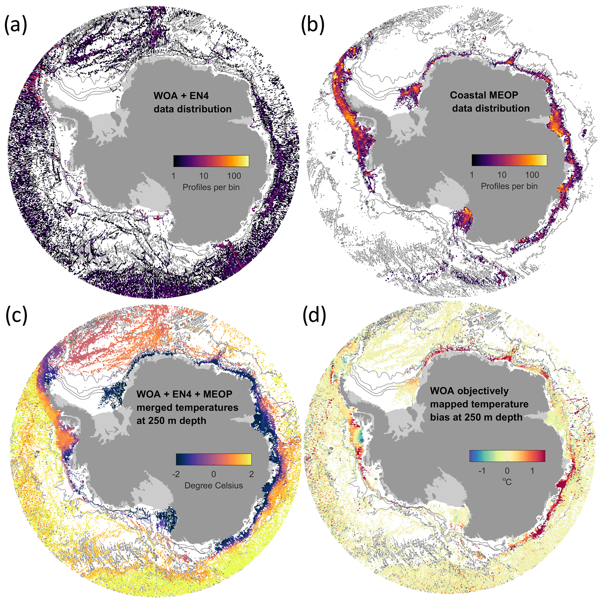
Figure 1 Circum-Antarctic coastal subsurface data distribution counted in 0.25^∘ bins from (a) combined World Ocean Atlas 2018 prerelease (WOA18p) and EN4 datasets and (b) MEOP seal profiles over areas shallower than 2500 m depth. (c) These datasets are combined to produce a sparse, merged climatological temperature dataset. (d) The difference between the WOA18p objectively analyzed temperature and the merged climatology reveals biases (mostly warm) on the Antarctic continental shelf in the former.

Data density maps and comparisons of the merged product with objectively analyzed WOA18p fields show significantly increased data coverage and reduction in bias in certain regions (Fig. 1). In particular, large parts of the narrow continental-shelf region surrounding East Antarctica show a subsurface warm bias on the order of 1 ^∘C in the WOA18p data, while a similar cold bias is evident in the Bellingshausen Sea sector. Obviously, those biases will affect parameterized melt rates that largely depend on the coastal ocean temperatures. In July 2019, well after this project was underway, a final version of the World Ocean Atlas 2018 was released (Locarnini et al., 2019) that also incorporated the MEOP observations. While the new WOA18 statistical means are close to those in our merged dataset, the objective analysis provided in WOA18 does not seem able to account for the strong horizontal gradients over the very narrow continental shelf of East Antarctica, which suggests that our merged dataset may be more adequate for providing continental-shelf properties for these regions (Fig. S1 in the Supplement).

Besides providing a reference of contemporary Antarctic coastal ocean temperature and salinity, the climatology obtained in the above method is used when computing the projected thermal forcing based on the CMIP future model anomalies. For this purpose, CMIP potential temperatures are converted to in situ temperature using the Gibbs SeaWater Oceanographic Toolbox of TEOS-10 (McDougall and Barker, 2011). Then, temperature and salinity fields are interpolated onto the standard grid. Anomalies are calculated as the difference between CMIP annual means and the CMIP 1995–2014 average and added to the observed climatology. This general methodology can be used to obtain ocean temperature and salinity anomalies for any CMIP model under any emission scenario, while the general strategy to select the CMIP5 models used in the ISMIP6 experiments is described in Barthel et al. (2020).

3.2 Extrapolation of ocean properties into the ice shelf cavities

The CMIP ocean model components typically include a coarse representation of the open ocean on the Antarctic continental shelf but do not explicitly resolve the circulation inside ice shelf cavities. Basal melt parameterizations such as those we propose for ISMIP6 require knowledge of the “ambient” ocean properties (i.e., ocean temperature and salinity unaffected by interactions with the melt plume), preferably as functions of depth within the ice shelf cavity. In addition, bathymetric features are known to control ocean properties in ice shelf cavities (De Rydt et al., 2014; De Rydt and Gudmundsson, 2016); deep troughs will make it easier for warmer, deeper water masses to reach into the cavity, while sills will tend to block them. Our goal is to allow temperature and salinity fields from the observed climatology and CMIP projections to flood into the ice shelf cavities and regions below sea level that are presently covered by glacial ice while accounting for topographic barriers.

To accomplish this, ocean model and observational data are first conservatively interpolated in the vertical to a 20 m regular grid, then bilinearly remapped in the horizontal onto the ISMIP6 standard grid. Next, the extrapolation algorithm described below is applied first in the open ocean (outside of present-day ice shelf cavities) and then in ice-covered regions of each of the 16 independent sectors (see Sect. 4.1 and Fig. 2). We assume that ice shelf cavities in separate sectors will remain disconnected from one another over the timescales of ISMIP6 runs so ocean properties are not interpolated across sectors. Note that because we perform extrapolation first in the open ocean and then in each basin, we do not use the portions of each basin in Fig. 2 that have been extended into the open ocean. The basins have only been extended for use by ISMIP6 ice sheet modelers, who may need the basins as part of the parameterizations described in Sect. 4.

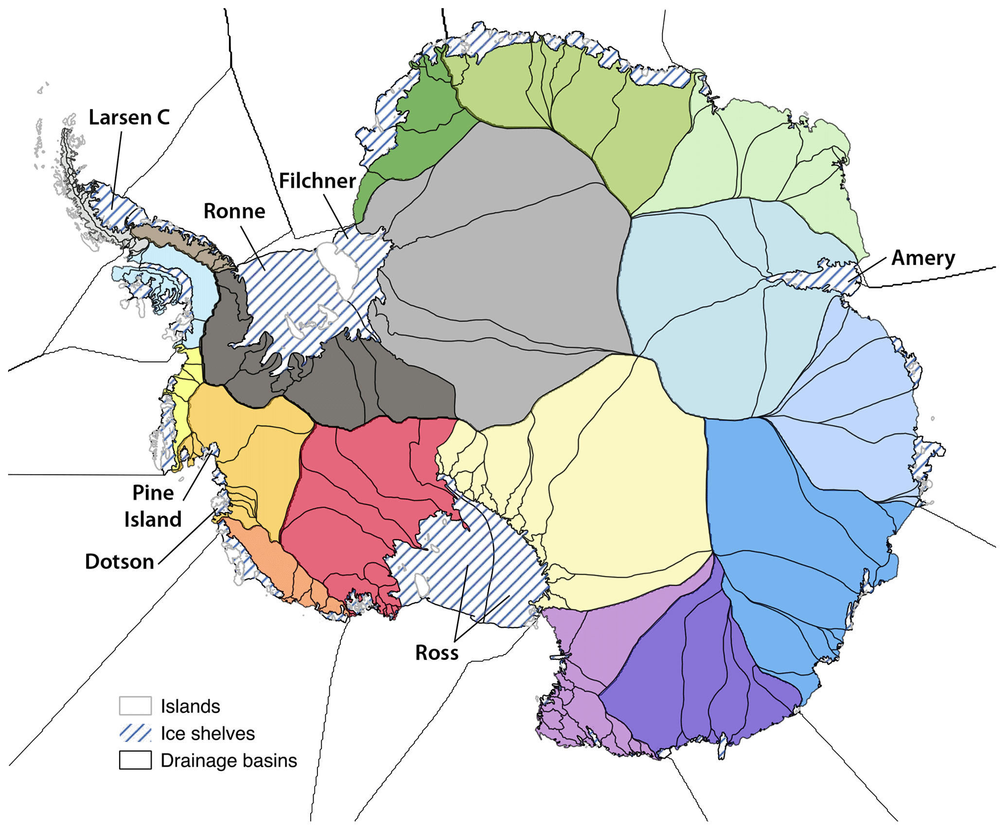
Figure 2 Eighteen Antarctic sectors (colors) defined by Mouginot et al. (2017) and Rignot et al. (2019). Individual drainage basins (black contours) are shown but are not used in this study.

In each basin, and separately in each horizontal layer, we convolve the resulting fields with a 2-D Gaussian kernel with a 1σ radius of 8 km to smooth the data at the grid scale and fill in missing values in open ocean. We allow this smoothing to extend the reach of the valid data by up to 12 km. This “flooding” only applies to regions where the bedrock topography, taken from Bedmap2 (Fretwell et al., 2013), is below the depth of the layer, meaning that bathymetric sills can block access of water masses deeper than the sill. This extrapolation via Gaussian smoothing is performed repeatedly, each time extending the reach of “valid” data by an additional 12 km, until no further cells with missing data can be reached. “Valid” data are only smoothed once in this process and are held fixed in subsequent iterations of the extrapolation process. We discovered that extrapolation by more than ∼12 km in one iteration results in unphysical mixing of qualitatively different water masses over narrow topographic features, including across the Antarctic Peninsula.

Deep ice shelf cavities blocked by sills will not be reached by purely horizontal extrapolation, so these deeper regions are filled in by copying the in situ temperature and salinity from overlying layers. Since ice sheet models will not necessarily use the Bedmap2 topography on the ISMIP6 standard grid as we have, we also copy ocean properties vertically below the bathymetry. This ensures that valid (and reasonable) values of ocean properties are available at all depths. To reduce the size of the final dataset, we conservatively interpolate from the 20 m vertical grid to a 60 m vertical grid.

We note that, in retrospect, we should have performed vertical extrapolation (that is, copying) using conservative temperature rather than in situ temperature because conservative temperature is the more appropriate quantity to remain constant with vertical advection. However, we estimate that this difference introduces an error in thermal forcing of no more than 0.1 K, which is certainly much smaller than other sources of uncertainty (observational errors, extrapolation, projection uncertainty, approximation error in the melt parameterization, etc.).

The extrapolation algorithm provides continuous, three-dimensional ocean fields that can be interpolated to any possible depth of the ice shelf base for use in the basal melt parameterization of the ISMIP6 models. This method keeps the same vertical structure inside ice shelf cavities as in the “ambient ocean” of observations or CMIP5 anomalies, which omits several physical processes. For example, the extrapolated “ambient” temperature inside of some of the large ice shelf cavities (e.g., Ross and Ronne–Filchner) are typically warmer than observed temperatures, which are often below the surface freezing point as a result of the high pressure and entrainment of meltwater. These processes are not represented in CMIP ocean models, which have no cavities, and there is no simple way of accounting for these in our extrapolation. Furthermore, the heat loss and freshwater input from ice shelf melting itself, the topographic steering by the ice draft topography, and the interaction of the buoyancy-driven flow in the cavity with the circulation outside of the cavity may result in feedback mechanisms that may increase or decrease the on-shore heat transport as a response to ice shelf melting (e.g., Swingedouw et al., 2008; Hattermann and Levermann, 2010; Jourdain et al., 2017; Hellmer et al., 2017; Bronselaer et al., 2018; Hattermann, 2018). Again, there is no simple way of including these processes in this effort. Finally, poor knowledge of bathymetry beneath many ice shelves may affect the accuracy of the extrapolated ocean properties (e.g., Schaffer et al., 2016; Millan et al., 2017). The resulting thermal forcing along the current ice shelf drafts is shown in Sect. 4.

4 Basal melting parameterization

As explained in Sect. 2, we suggest a relatively simple parameterization for the ISMIP6 standard experiments. The current understanding of ice–ocean interactions suggests that the total ice shelf basal melt increases quadratically as the ocean, offshore of the ice front, warms (Holland et al., 2008). However, ice sheet models require melt rates at each location underneath ice shelves, not just the total melt rate. A first possibility is to make the melt rate proportional to the square of the local thermal forcing. Such a “local” parameterization implicitly assumes that the melt-induced circulation develops locally to reinforce turbulence and subsequent melting. However, there is evidence that the melt-induced circulation develops at the scale of the ice shelf cavity (e.g., Jourdain et al., 2017). For this reason, Favier et al. (2019) suggested parameterizing melt rates as the product of the local thermal forcing (to keep the influence of ocean stratification) and the nonlocal thermal forcing (i.e., averaged over the entire ice shelf base to account for the cavity-scale, melt-induced circulation). For simplicity and consistency with Favier et al. (2019), we refer to this parameterization as “nonlocal,” although it includes a mix of local and nonlocal thermal forcing. A fully nonlocal parameterization would be similar to that of DeConto and Pollard (2016): a single ocean temperature used to calculate the melt rates at every point of the ice shelf base.

The optimal parameterization identified for this effort is the nonlocal parameterization, which was found to best reproduce the results from coupled ice sheet–ocean models in an idealized context (Favier et al., 2019). Because of its nonlocal nature, however, the implementation of this parameterization in ice sheet models may be complicated (mostly because of parallel computations). As a result, for ice sheet models unable to implement this nonlocal parameterization, the recommendation is to use the local version instead. These two basal melt parameterizations are described below. We first start by defining regional sectors used to calibrate the parameters.

4.1 Regional sectors

Given that melt rates have been estimated for more than 60 individual ice shelves (Rignot et al., 2013), we could in theory calibrate the parameterizations with different parameters in each cavity. However, ice sheet models have evolving cavities, and their present-day ice shelves and ice flows do not necessarily correspond to the observed ones, depending on their initialization method (Seroussi et al., 2019). Furthermore, two initially distinct ice shelves may merge at some future time (e.g., Pine Island and Thwaites), leading to melt discontinuities if parameters are set at the scale of individual drainage basins. Therefore, we choose to calibrate parameters at the scale of larger sectors.

We start from the 18 sectors used in the latest ice sheet mass balance inter-comparison exercise (IMBIE) assessment (Shepherd et al., 2018) and based on drainage basin boundaries defined from satellite ice sheet surface elevation and velocities (Mouginot et al., 2017; Rignot et al., 2019). To obtain continuous melt rates underneath all the ice shelves, we merge the two sectors feeding the Ross ice shelf and the two sectors feeding the Ronne–Filchner ice shelf (Fig. 2). To allow simulated ice shelves to be larger than currently observed, the 16 remaining sectors are then extended into the open ocean over the full ISMIP6 standard grid by finding the basin of the closest ice-covered point to a given point in the open ocean.

4.2 Nonlocal quadratic melting parameterization

Melt rates in the common ISMIP6 experiments are derived using a slightly modified version of the nonlocal quadratic parameterization proposed by Favier et al. (2019). The parameterization is explicitly defined over regional sectors rather than for a single ice shelf, and it includes a temperature correction:

$$\begin{array}{}\text{(1)}& \begin{array}{rl}m(x,y)& ={\mathit{\gamma }}_{\mathrm{0}}\times {\left({\displaystyle \frac{{\mathit{\rho }}_{\mathrm{sw}}{c}_{\mathrm{pw}}}{{\mathit{\rho }}_{\mathrm{i}}{L}_{\mathrm{f}}}}\right)}^{\mathrm{2}}\\ & \times \left(\mathrm{TF}(x,y,z_{\mathrm{draft}})+\mathit{\delta }{T}_{\mathrm{sector}}\right)\\ & \times \left|\langle \mathrm{TF}{\rangle }_{\mathrm{draft}\in \mathrm{sector}}+\mathit{\delta }{T}_{\mathrm{sector}}\right|,\end{array}\end{array}$$

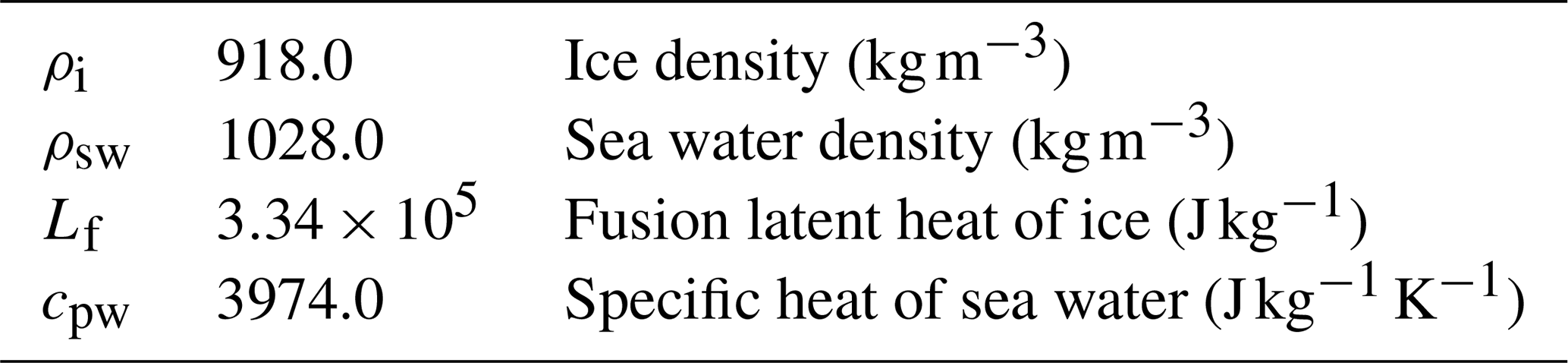
where $\mathrm{TF}(x,y,z_{\mathrm{draft}})$ is the thermal forcing at the ice–ocean interface, and 〈TF〉_{draft∈sector} is the thermal forcing averaged over all the ice shelves of an entire sector. The uniform coefficient γ₀, with units of velocity, is somewhat similar to the exchange velocity commonly used to calculate ice–ocean heat fluxes (e.g., Holland and Jenkins, 1999; Jenkins et al., 2010). The temperature correction δT_sector for each sector is needed to reproduce observation-based melt rates (at the scale of a sector) from observation-based thermal forcing. The other constants are given in Table 1.

Table 1 Physical constants used in the melt parameterizations.

The temperature correction is introduced to account for biases in observational products, ocean property changes from the continental shelf to the ice shelf base (not accounted for in the aforementioned extrapolation), tidal effects, and other missing physics. A similar correction was used by Lazeroms et al. (2018). Because of the quadratic dependency of parameterized melt to thermal forcing, the melting sensitivity to ocean warming (i.e., the derivative) linearly depends on the present-day thermal forcing, which is a strong incentive to apply a temperature correction. Without temperature correction, a sector-dependent γ coefficient would be required to simulate the observation-derived melt rates in each sector. This approach would lead to γ ranging from 500 to 60 000 m yr⁻¹ in the different sectors, which seems difficult to justify with physical arguments. Differences across ice shelves in how efficiently available heat is converted to melting are expected as the melt-induced circulation may respond differently to a given thermal forcing depending on its specific geometry (e.g., Jenkins, 1991; Little et al., 2009; Jourdain et al., 2017) and on regional contrasts in the amplitude of tides (Padman et al., 2018). However, tides and cavity geometry unlikely account for efficiencies across ice shelves that differ by 2 orders of magnitude. Furthermore, as γ explains most of the melt sensitivity to increasing thermal forcing (see Eq. 1), an approach with sector-dependent γ would produce sensitivities to future ocean warming that would be strongly influenced by the regional biases in the observational products used to estimate γ. For these reasons, we think that a constant γ₀ for all of Antarctica is preferable for ISMIP6.

4.3 Local quadratic melting parameterization

The nonlocal parameterization involves spatial integration, which may not be straightforward to implement for all the modeling groups. For those models which cannot implement the nonlocal parameterization, we propose a local version:

$$\begin{array}{}\text{(2)}& \begin{array}{rl}m(x,y)& ={\mathit{\gamma }}_{\mathrm{0}}\times {\left({\displaystyle \frac{{\mathit{\rho }}_{\mathrm{sw}}{c}_{\mathrm{pw}}}{{\mathit{\rho }}_{\mathrm{i}}{L}_{\mathrm{f}}}}\right)}^{\mathrm{2}}\\ & \times {\left\{\max \left[\mathrm{TF}(x,y,z_{\mathrm{draft}})+\mathit{\delta }{T}_{\mathrm{sector}},\mathrm{0}\right]\right\}}^{\mathrm{2}},\end{array}\end{array}$$

in which the max function is preferred to the absolute value of the last term on the right in order to avoid extreme melt rates when adjusting parameters in areas with both melting and refreezing.

4.4 Calibration of γ₀ and δT_sector and related uncertainty

We propose two calibration methods that provide both present-day, sector-integrated melt rates equal to observational estimates and different melt patterns and sensitivities to ocean warming. These two calibration methods are applied to both the local and nonlocal parameterizations. For both methods, the calibration is done in two stages. First, it is assumed that δT_sector=0 in every sector, and we estimate γ₀ based on observational constraints specific to each method. Then we calibrate δT_sector to obtain present-day, sector-integrated melt rates equal to observational estimates. For all these estimates, we use temperatures and salinity from the climatological dataset described in Sect. 3 and the ice shelf geometry from Bedmap2 (Fretwell et al., 2013).

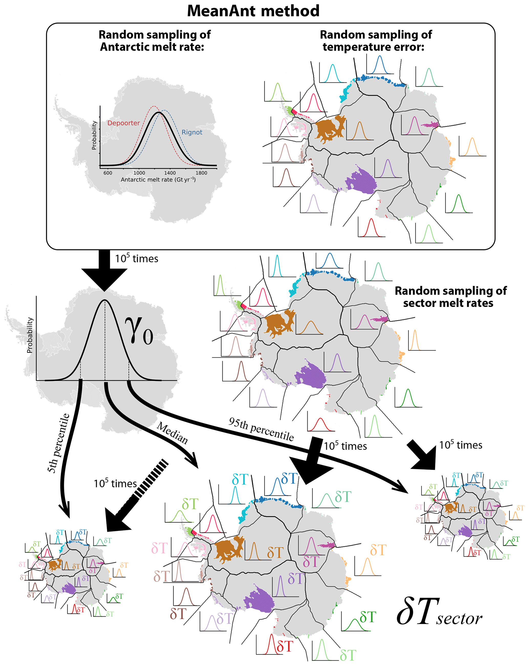
Figure 3 The MeanAnt method used to calibrate γ₀ and δT_sector. The γ₀ coefficient is obtained from distributions of the total Antarctic ice shelf basal mass loss and of thermal forcing with coherent normal errors in each sector (upper frame). For each resulting γ₀ value, the δT coefficients are introduced to obtain the ice shelf basal mass loss in individual Antarctic sectors.

In the “MeanAnt” method, γ₀ is calibrated in such a way that the parameterization reproduces the total Antarctic melt rate with no thermal forcing correction, i.e., 1325±175 Gt yr⁻¹ (Rignot et al., 2013) or 1193±163 Gt yr⁻¹ (Depoorter et al., 2013), where ± indicates standard deviation. To estimate a distribution of possible γ₀ values, we take 10⁵ random samples in both the total Antarctic melt rate and the error in thermal forcing using normal distributions based on the aforementioned melt values (equally sampling Rignot and Depoorter's datasets; Rignot et al., 2013; Depoorter et al., 2013) and assuming an uncertainty of 0.17 K for the ocean thermal forcing. Using 10⁵ samples gives percentiles of the γ₀ distribution that converge with three significant digits. The 0.17 K uncertainty was calculated as the average temperature standard deviation at 500 m depth, between 80 and 60^∘ S, only considering locations with more than three valid points in the original dataset (Sect. 3) and neglecting the uncertainty in salinity in the calculation of freezing temperature. The random error applied to the ocean thermal forcing is sampled once per sector, i.e., we assume coherent errors at the scale of a sector, and the sector random error is added to the grid point thermal forcing. The MeanAnt method is summarized in Fig. 3.

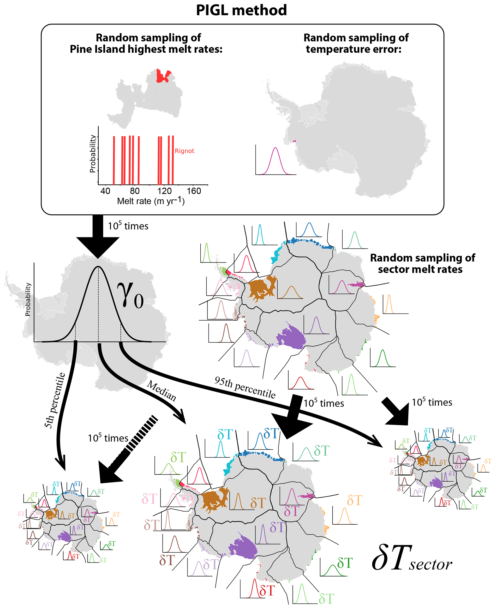
Figure 4 PIGL method used to calibrate γ₀ and δT_sector. The γ₀ coefficient is obtained by randomly sampling 1 of the 10 grid points with highest melt rates (red area in the upper left figure) beneath the Pine Island ice shelf (gray area in the upper left figure) and normally distributed thermal forcing. For each resulting γ₀ value, the δT coefficients are then introduced to obtain the ice shelf basal mass loss in individual Antarctic sectors.

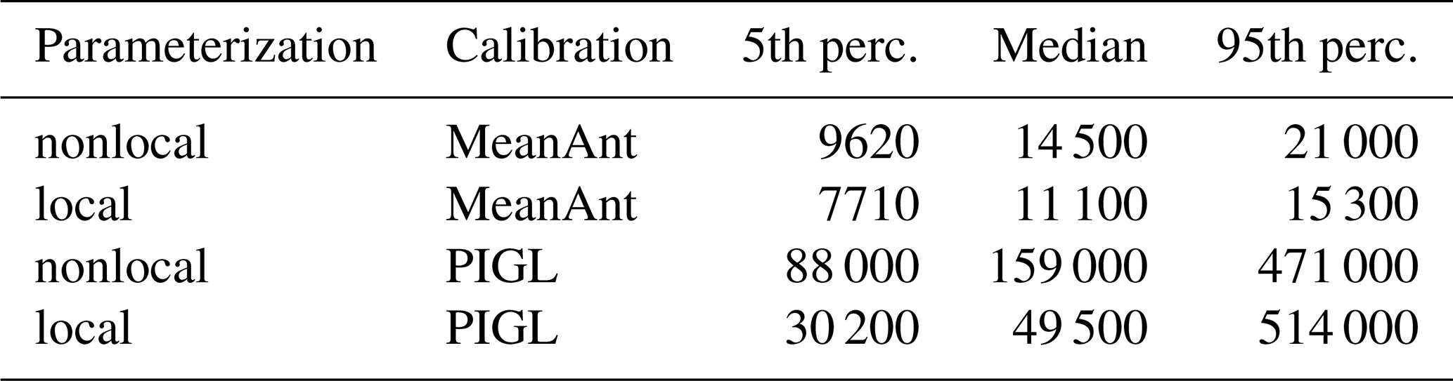
The idea behind the second method, hereafter “PIGL”, is that total Antarctic melt rate may be less relevant than melt rates near deep grounding lines for ice sheet dynamics (Reese et al., 2018b). We assume that the highest melt rates of Antarctica, found near Pine Island's deep grounding line, as well as the relatively high number of ocean observations in the Amundsen Sea provide a constraint on how Antarctic melt rates could respond to strong future ocean warming. In the PIGL method, we therefore use the spatial pattern of melt rates provided byRignot et al. (2013; here version 2.1 of their product is used), and we estimate γ₀ by randomly sampling one of the 10 grid points with the highest melt rates (with equal probability) and associated thermal forcing (normally distributed uniform error over the entire Amundsen basin) underneath the Pine Island ice shelf. This is repeated 10⁵ times to obtain the median, 5th, and 95th percentiles of γ₀. The PIGL method is summarized in Fig. 4. The values obtained through the PIGL method are an order of magnitude greater than through the MeanAnt method, and the two distributions do not overlap (Table 2). The PIGL median and 5th percentile γ₀ values are 3 times higher for the nonlocal than for the local parameterization, which can be explained by the presence of refreezing in the first case, requiring a large γ₀ to compensate small sector-averaged thermal forcing. For PIGL local, the 95th percentile γ₀ takes values as large as the nonlocal case because δT corrections become strongly negative and make the max function in Eq. (2) produce zero melt at numerous grid points.

Table 2 Calibrated γ₀ values for the two quadratic parameterizations and the two calibration methods (m yr⁻¹).

In the following, the parameterizations and calibration methods are sometimes referred to as “nonlocal MeanAnt” and “nonlocal PIGL” and similarly for the local version.

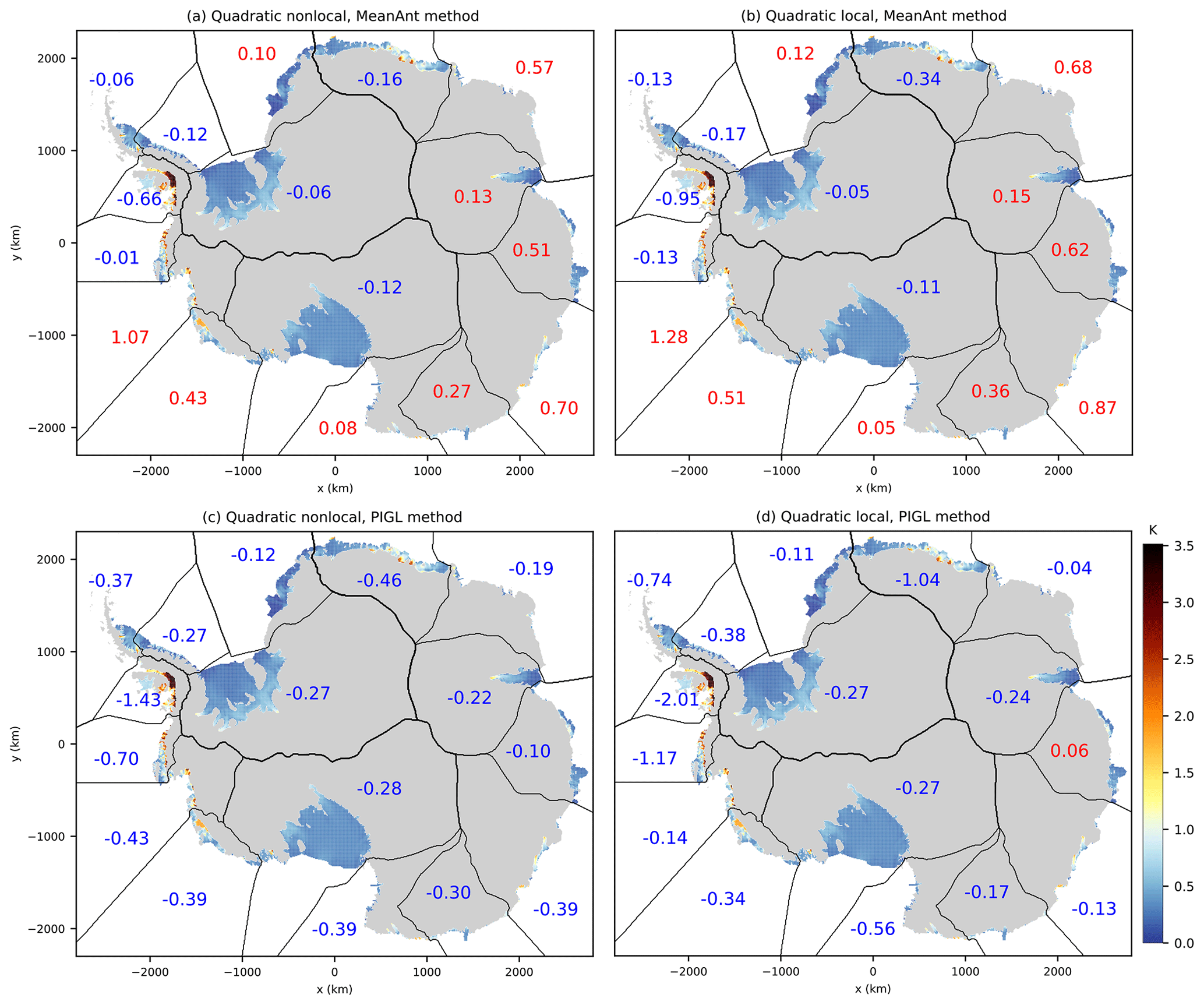
Figure 5 Thermal forcing along the ice shelf bases (shaded) and median δT corrections in each sector (numbers; negative in blue, positive in red) associated with median γ₀ estimates for the two proposed parameterizations and two calibration methods.

Then, we determine δT in each sector by iterations. For each specific γ₀ value (e.g., median), we estimate δT 10⁵ times by randomly sampling the sector-integrated melt rates (Gt yr⁻¹) in normal distributions. Random errors are sampled independently for each ice shelf within a sector when using the melt rates from Rignot et al. (2013), with a normal distribution defined by the means and standard deviations given in their Table 1. When using melt rates from Depoorter et al. (2013), random errors are sampled independently for each sector described in their supplementary Table 1. The median δT values corresponding to the median of the γ₀ distributions are shown in Fig. 5. We note that MeanAnt δT values are positive and negative by construction, while PIGL δT values are negative, as expected if this correction represents changes in water mass properties along the ice draft (keeping in mind that it also likely accounts for missing physics). Median δT values corresponding to the 5th and 95th percentiles of the γ₀ distributions are provided in the ISMIP6 repository (see data availability section).

After this two-stage calibration, we have a distribution of γ₀ for the whole ice sheet and distributions of δT for each sector. The ISMIP6 protocol (Nowicki et al., in preparation) explicitly requires exploration of the sensitivity of ice sheet projections to γ₀ using various γ₀ values from Table 2 but taking the median δT values obtained for a given value of γ₀. These experiments will thus highlight the uncertainty in the sensitivity of melting to ocean warming but for experiments that all start from the median observed melt rates. To further explore parameter uncertainty (beyond ISMIP6 experiments), it could be interesting to randomly sample δT independently in each sector and for each γ₀ value to obtain a range of possible melt rates for their initial states, which would require running a much larger number of experiments to really sample the uncertainty in the different sectors.

To summarize, we suggest using either the nonlocal or the local quadratic parameterization in ISMIP6. For any of them, we recommend using two sets of parameters to account for the large uncertainty in parameterized melt rates: (i) the MeanAnt parameters, giving a sensitivity to ocean warming based on the present-day relationship between temperatures and the mean Antarctic melt rate, and (ii) the PIGL parameters, giving a sensitivity to ocean warming based on present-day high thermal forcing and melt rates near Pine Island's grounding line.

5 Results

5.1 Present-day melt rates

To illustrate the differences between the two calibration methods, we first consider the example of the nonlocal parameterization applied to the Ronne–Filchner and Amundsen sectors that are cold and warm, respectively (Fig. 6a). Without applying the thermal forcing correction (i.e., considering δT=0), the MeanAnt method produces melt rates in good agreement with observations between 400 and 1000 m in the Ronne–Filchner sector (dashed light-blue line in Fig. 6b) but underestimates melt rates at all depths in the warm cavities of the Amundsen sector by 1 order of magnitude (dashed red line in Fig. 6b) and in the deepest parts of Ronne–Filchner. Adding δT=1.07 K brings the Amundsen Sea sector-averaged value close to the observational estimate (solid light-red line in Fig. 6b), while no substantial correction is needed for Ronne–Filchner. Without δT correction, the PIGL method fits the highest melt value of Pine Island but overestimates melt rates in all cavities, imposing δT<0 almost everywhere (Fig. 5). The MeanAnt method underestimates melt rates near the deepest parts of grounding lines for both the Amundsen and Ronne–Filchner sectors even after the thermal forcing correction. On the other hand, the PIGL method produces higher melt rates in the deepest parts of ice shelf cavities, which is in better agreement with observational estimates but yields to significantly underestimated melt rates at shallower depths (Fig. 6c).

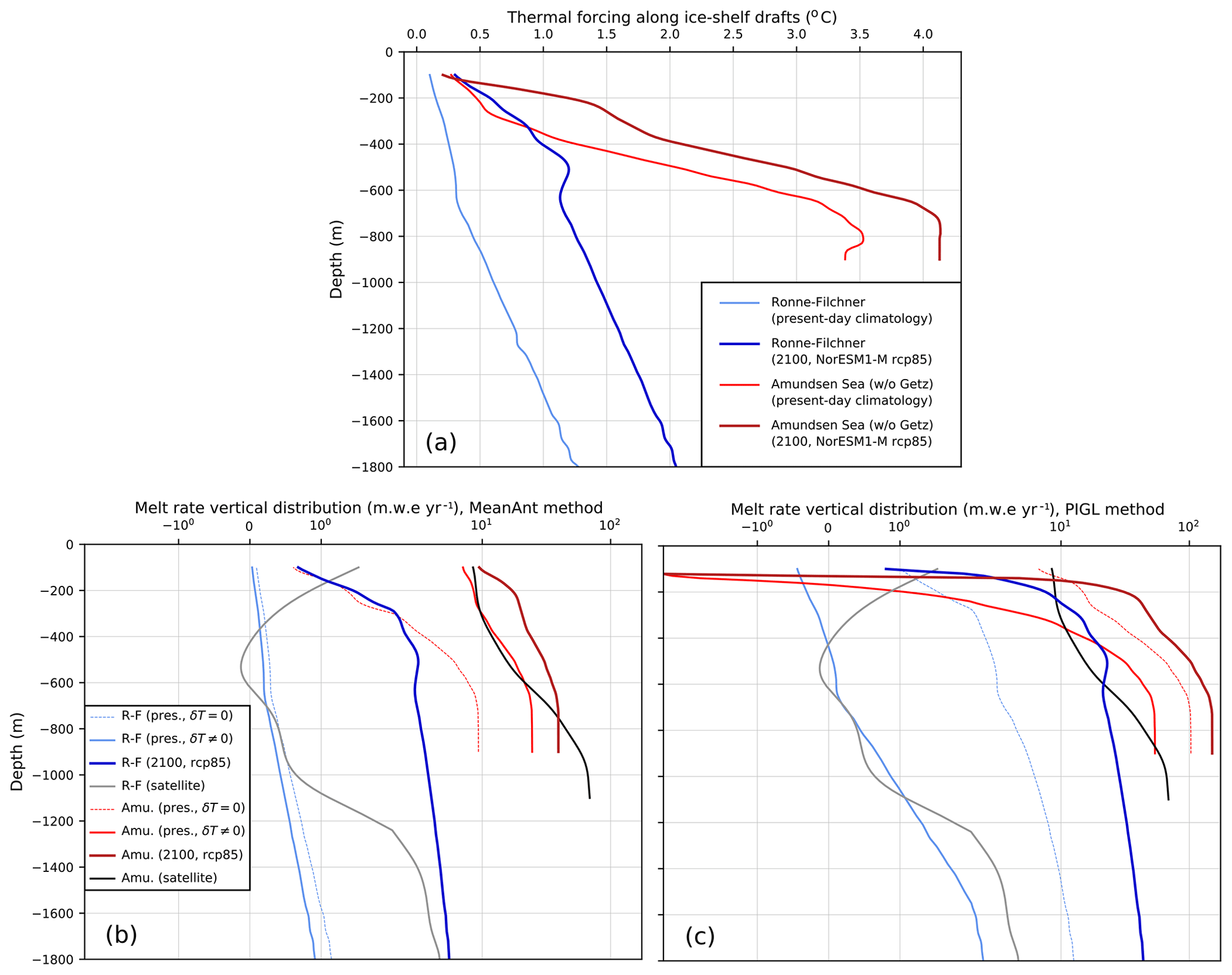
Figure 6 (a) Vertical distribution of present-day and future thermal forcing interpolated on the ice shelf bases for the Ronne–Filchner sector (blue) and the Amundsen sector, covering the ice shelves from Cosgrove to Dotson, i.e., not including Getz (red). Dark colors indicate projections. (b, c) Vertical distribution of present-day and future parameterized melt rates; the parameterized values obtained with no thermal forcing correction (δT=0) are shown as dashed lines; the equivalent distribution for satellite-based estimates (Rignot et al., 2013; update v2.1) is shown in gray (Ronne–Filchner) and black (Amundsen). The two panels illustrate the nonlocal parameterization for the two calibration methods. The mean profiles are estimated through a Gaussian kernel density estimate.

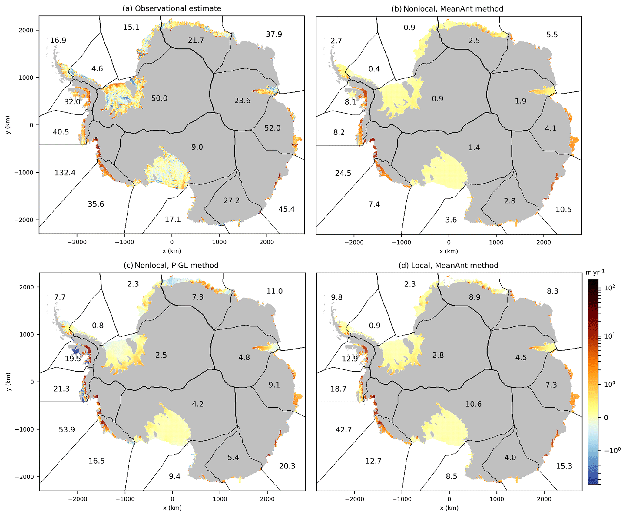
Figure 7 Present-day melt rates from (a) the observational estimate obtained by Rignot et al. (2013; update v2.1), (b) the quadratic nonlocal parameterization with the MeanAnt calibration method, (c) the quadratic nonlocal parameterization with the PIGL calibration method, and (d) the quadratic local parameterization with the MeanAnt calibration method. The numbers indicate maximum melt rates in individual sectors. The grounded ice sheet is shown in gray, and the black contours indicate the sectors used in this study.

We now assess parameterized melt rate patterns for the entire Antarctic ice sheet in comparison to the observational melt patterns from Rignot et al. (2013), as shown in Fig. 7a. The general picture is that nonlocal MeanAnt produces relatively uniform melt rates within individual sectors, with maximum present-day melt rates below 25 m yr⁻¹ (Fig. 7b). Nonlocal PIGL produces sharper gradients, with significantly larger maximum values near grounding lines (up to 54 m yr⁻¹; Fig. 7c). As in the observational product, nonlocal PIGL produces refreezing areas in some sectors but generally not at exactly the same location (e.g., Ronne, Dröning Maud Land). In the Bellingshausen Sea, areas of significant refreezing (3–4 m yr⁻¹) are produced by nonlocal PIGL, while observations suggest no significant refreezing in that sector. The local version produces sharper gradients than the nonlocal with no refreezing (by construction in Eq. 2), and maximum melt rates reach 43 m yr⁻¹ for the MeanAnt method (Fig. 7d) and 93 m yr⁻¹ for the PIGL method (not shown) in the Amundsen Sea sector.

While melt patterns are often used to assess basal melting parameterizations, assessing their ability to capture the interannual variability of melt rates is also valuable. The only region where both measured T,S profiles and observational estimates of cavity melt rates are available for multiple years (thus allowing an assessment of interannual variability) is the Amundsen Sea, in particular the Pine Island (Dutrieux et al., 2014) and Dotson (Jenkins et al., 2018) ice shelves. We use these T,S profiles to parameterize melt rates based on the aforementioned methods and compare them to observational estimates (based on meltwater fluxes estimated from T,S sections under the geostrophic assumption). This comparison is not a perfect evaluation of the ISMIP6 protocol as there is no observation to estimate the average thermal forcing over the entire Amundsen sector, and we therefore need to apply the parameterization over a single cavity rather than a larger sector. This affects the sector-averaged thermal forcing in the nonlocal case, with 1.40 ^∘C and 1.09 ^∘C for Pine Island and Dotson, respectively, vs. 1.07 ^∘C for the Amundsen sector as a whole. Therefore, δT needs to be recalibrated to get the present-day melt rate and the correct sensitivity to ocean warming (see Sect. 4.2). Another reason to recalibrate δT in this comparison is that the observational conductivity, temperature, and depth (CTD) profiles give much higher cavity-mean thermal forcing (2.27 and 1.62 ^∘C for Pine Island and Thwaites, respectively) than in the new climatological dataset (1.40 and 1.09 ^∘C). Using the ISMIP6 thermal corrections would lead to an overestimation of both present-day melting and sensitivity to temperature variations. The comparison is nonetheless useful to assess the behavior of such simple quadratic formulations and the γ₀ values used in the ISMIP6 protocol. For Pine Island, there is little agreement between the parameterized and observational variabilities, e.g., the parameterizations do not reproduce the observational peak in 2007 (Fig. 8a). In contrast, the parametrizations capture the increasing melt rate from 2000 to 2009 in Dotson, followed by a decrease and relatively stable melt rate over 2012–2016 (Fig. 8b). For both cavities, the MeanAnt method significantly underestimates the amplitude of interannual variability, while the PIGL method is close to the observational amplitude. These results are somewhat consistent with Favier et al. (2019), who tuned γ₀ without thermal correction to reproduce the mean melt rate of an idealized warm cavity and obtained γ₀ values in between the MeanAnt and PIGL values.

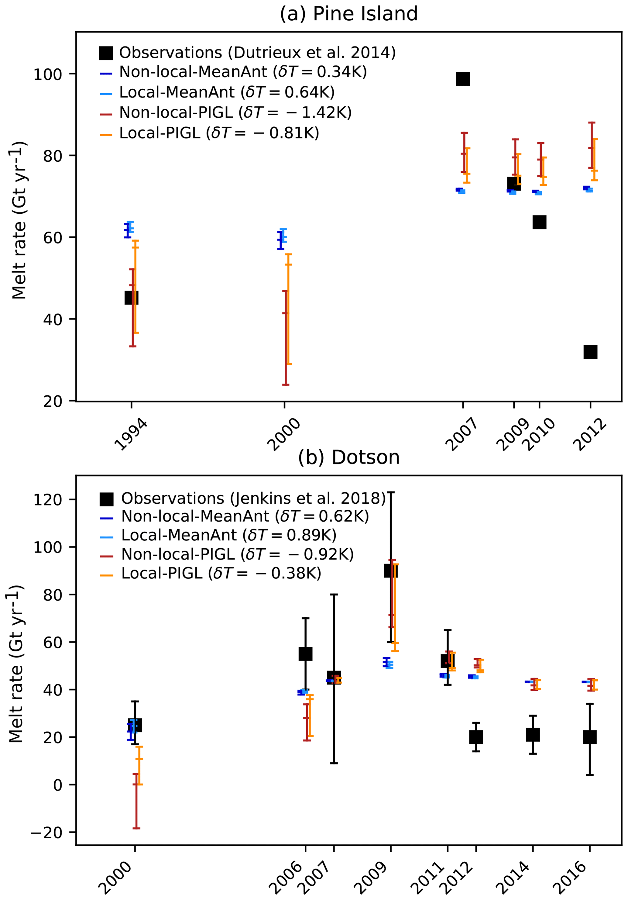
Figure 8 Interannual variability of observational and parameterized mean melt rates for (a) Pine Island and (b) Dotson cavities. Parameterized melt rates are calculated from the temperature and salinity profiles shown in Fig. 2a of Dutrieux et al. (2014) and Fig. 2a, b of Jenkins et al. (2018). For this figure, γ₀ has the standard values that are calculated for the whole Antarctic ice sheet. Keeping the δT previously determined for the Amundsen sector would not make sense as sector-averaged thermal forcing must be replaced by ice-shelf-averaged thermal forcing for this comparison. Therefore, for this plot, δT is calibrated to match the mean observational cavity melt rate, and the sector-averaged thermal forcing used in the nonlocal parameterizations is replaced with the cavity-averaged thermal forcing. The error bars of parameterized melt rates arise from the use of γ₀'s 5th, 50th, and 95th percentiles.

5.2 Example of future melt rates

Here we illustrate the ocean forcing protocol by deriving future melt rates under the Antarctic ice shelves from six CMIP5 models, considering the r1i1p1 ensemble member of CCSM4, CSIRO-mk3-6-0, HadGEM2-ES, IPSL-CM5A-MR, MIROC-ESM-CHEM, and NorESM1-M. These projections are to be considered as zero-order approximations because the depth and extent of ice shelves in the ice sheet simulations are expected to change in response to the evolving ice dynamics as well as basal and surface mass balance, which is not taken into account here. The changing geometry will be accounted for in the final ISMIP6 ice sheet projections, with all forcings combined to ice sheet dynamics (Nowicki et al., in preparation).

As illustrated in Fig. 9 for a single CMIP5 model (NorESM1-M; Iversen et al., 2013), the mean Antarctic ice shelf melt rate can be estimated throughout the historical period (1850–2005) and for Representative Concentration Pathway (RCP) scenarios (2006–2100), accounting for parameter uncertainty. The early part of the historical period is close to the preindustrial state and can be used for the long spin-up period that is sometimes needed to initialize ice sheet models. For the NorESM1-M model, the mean melt rate remains close to the observational estimate (0.85 m w.e. yr⁻¹) under the rcp26 scenario. In contrast, the mean melt rate is strongly enhanced at the end of the 21st century under rcp85, reaching ∼6 m w.e. yr⁻¹ with nonlocal MeanAnt and ∼40 m w.e. yr⁻¹ with nonlocal PIGL (median values).

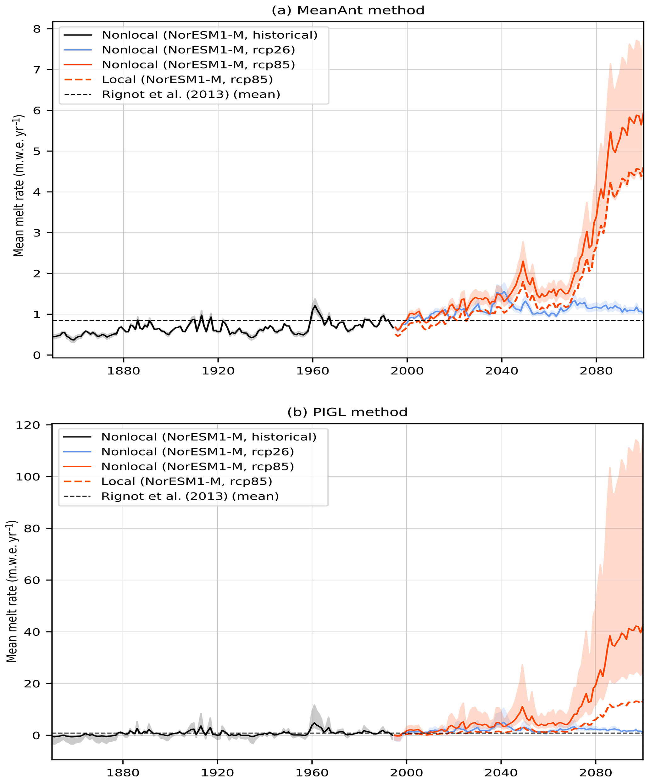
Figure 9 Time series of mean Antarctic ice shelf basal melt rates (using the nonlocal parameterization and assuming a static ice sheet geometry) based on the nonlocal parameterization, calibrated following (a) the MeanAnt method and (b) the PIGL method and obtained from the NorESM1-M CMIP5 simulations. The semitransparent area indicates the 5–95th percentile range related to the uncertainty in γ₀. Note the different amplitudes for the melt rates.

Returning to Fig. 6, we can see how the calibration method affects projected melt rates in the Ronne–Filchner and Amundsen sectors, which both undergo ∼0.75 ^∘C warming at depth: as for present day, the PIGL method produces much stronger future melt rates at depth than the MeanAnt method (43 vs. 5 m yr⁻¹ for Ronne–Filchner at 1800 m depth and 150 vs. 39 m yr⁻¹ for Pine Island at 900 m depth).

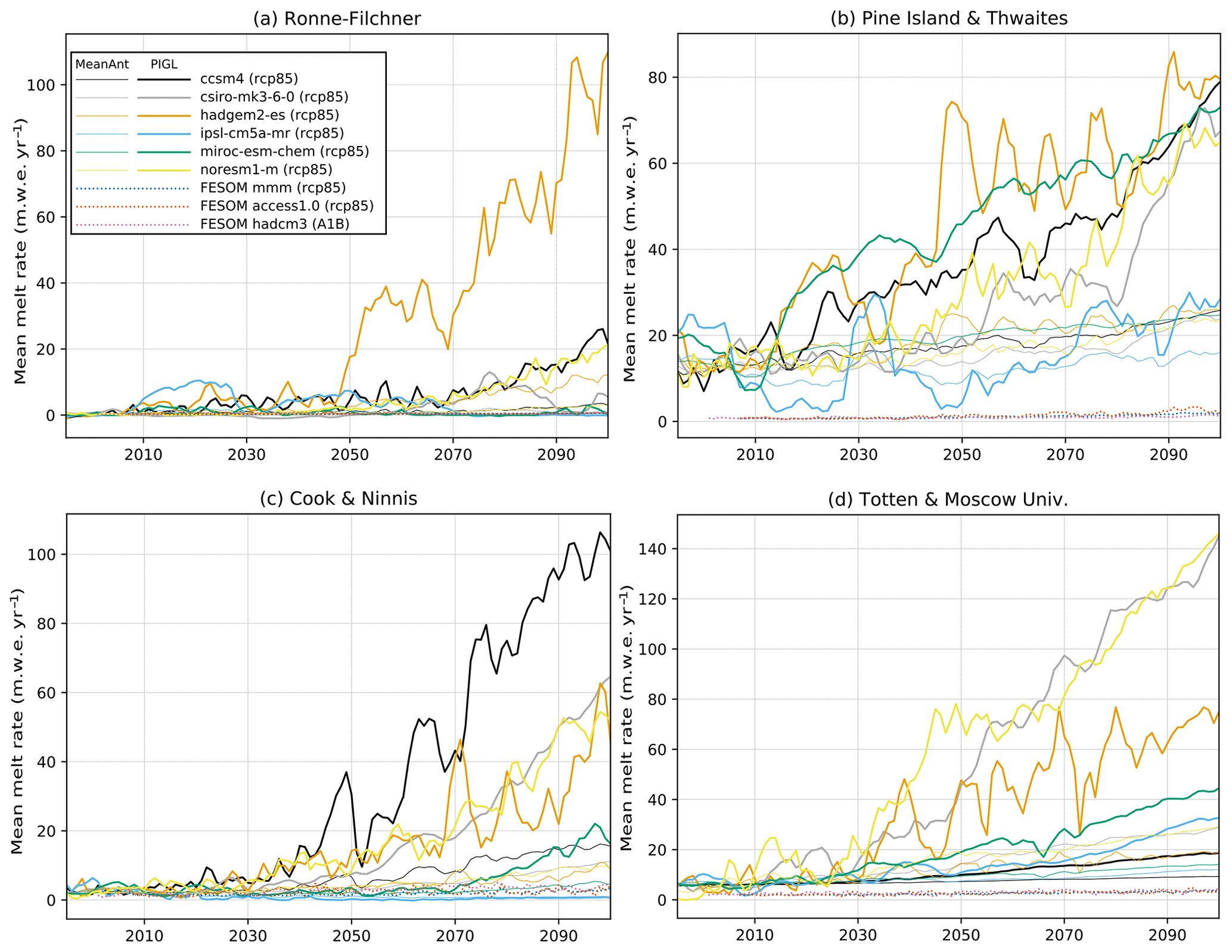
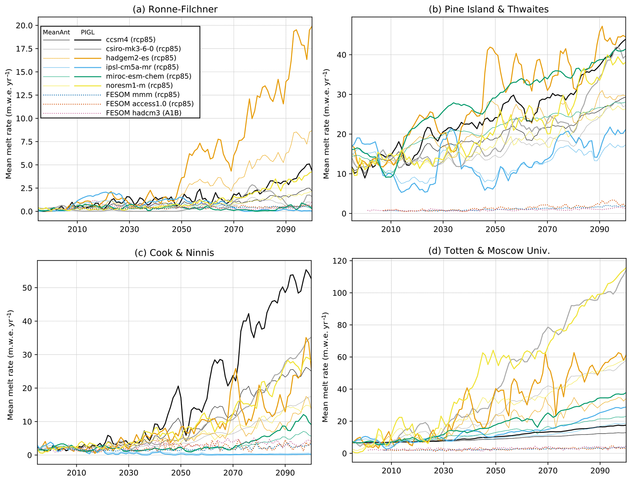
Figure 10 Time series of mean cavity basal melt rates over the 21st century under the rcp85 scenario for (a) Ronne–Filchner, (b) Pine Island and Thwaites, (c) Cook and Ninnis, and (d) Totten and Moscow University. The projection is shown for six CMIP5 models with both the MeanAnt (thin lines) and PIGL (thick lines) calibrations. The average over 1995–2014 corresponds to the observational estimates. Three projections from the FESOM ocean model (resolving ice shelf cavities) are included; they are forced by atmospheric fields from either the ACCESS-1.0 or the CMIP5 multimodel mean (MMM) as described by Naughten et al. (2018a) or from the CMIP3 HadCM3 model as described by Timmermann and Hellmer (2013).

We now consider projections from six CMIP5 models under the rcp85 scenario in four different regions where ice shelves buttress a large volume of ice grounded below sea level, here only considering the nonlocal parameterization (Fig. 10). For Pine Island and Thwaites, all models but IPSL-CM5A-MR indicate an increase in mean melt rate by a factor of ∼1.5 (MeanAnt) to ∼4.5 (PIGL) in 2100. The relative increase for the three other regions is much larger: based on PIGL parameters, a majority of CMIP5 models give projected melt rates exceeding the present-day Pine Island and Thwaites mean values (∼17 m yr⁻¹) before 2100, even exceeding 100 m yr⁻¹ for some models. The MeanAnt parameters give weaker increases for these three regions, with melt rates underneath Ronne–Filchner remaining below 3 m yr⁻¹ in all models but HadGEM2-ES and half of the models reaching ∼10 m yr⁻¹ underneath Cook and Ninnis and ∼20 m yr⁻¹ underneath Totten and Moscow University by 2100.

Comparing these results to projections from ocean models that represent ice shelf cavities can be used to assess projections from the proposed parameterizations. Such model projections were done for CMIP3 and CMIP5 models by Timmermann and Hellmer (2013) and Naughten et al. (2018a), respectively, using the Finite Element Sea Ice–Ocean Model (FESOM). The FESOM simulations produce realistic present-day melt rates beneath Ronne–Filchner, and their projected melt rates are close to the low end of the CMIP5 distribution for nonlocal MeanAnt. By contrast, half of the CMIP5 models used through nonlocal PIGL give melt rates above 20 m yr⁻¹, which is far above FESOM projections for 2100 (Fig. 10a), and still far above the 6 m yr⁻¹ in 2200 under much warmer conditions (Timmermann and Hellmer, 2013). This could suggest that our melting parameterization is too sensitive to warming (overestimated γ₀), although this is not what is suggested by our previous analysis of Dotson and Pine Island interannual variability (Fig. 8). Alternatively, it could mean that projected ocean warming is largely overestimated by some CMIP5 models in the Weddell Sea.

In contrast to Ronne–Filchner, present-day melt rates produced by FESOM were significantly underestimated in other cavities, as reported by Timmermann and Hellmer (2013) and Naughten et al. (2018a). For example, the underestimation reached a factor of 10 beneath Pine Island and Thwaites as well as beneath Totten and Moscow University (see dotted lines in Fig. 10), mostly due to overly strong convection and to the subsequent presence of cold water in these regions, as discussed by Naughten et al. (2018b, a). These strong present-day biases make it difficult to use these ocean simulations as a reference to assess projections from the proposed parameterizations.

FESOM is the only model so far that has been used to build CMIP-based projections of ice shelf melting. Seroussi et al. (2017) have run more idealized projections, adding +0.5 ^∘C to the initial state and lateral boundary conditions of a regional ocean simulation centered on the eastern Amundsen Sea. We use their simulation to evaluate the sensitivity of melt rates to warming beneath Thwaites glacier (Fig. 11). The comparison is made by adding +0.5 ^∘C to the present-day thermal forcing in the entire Amundsen sector and using the standard ISMIP6 values for γ₀ and δT. It is again not easy to conclude which parameterization performs better. First of all, the present-day parameterized values are underestimated compared to Seroussi et al. (2017) and to the observations. MeanAnt seems to be in better agreement with Seroussi et al. (2017) in terms of relative increase for both average and high-end values, but the warm state of nonlocal PIGL is quite close to the warm state in Seroussi et al. (2017). The change in melt rates is probably more relevant for ISMIP6 than the initial value as the ISMIP6 results are presented with respect to control simulations (Seroussi et al., 2020), which would suggest that the MeanAnt sensitivity is correct in the Amundsen Sea.

Figure 11 (a) Mean basal melt rate beneath Thwaites at present day (blue) and with a +0.5 ^∘C anomaly (dark red), as simulated over the first 20 years of Seroussi et al. (2017)'s simulation, and as parameterized through the ISMIP6 protocol. (b) Same as panel (a) but showing the 90th percentile of the melt spacial distribution. The diagram represent median values, and the black bars indicate the 5th and 95th percentiles. Note that the 90th percentile of the melt spacial distribution can be zero due to the max function used in the local parameterization.

6 Discussion and conclusion

In this paper, we have combined three available datasets (MEOP, WOA18 prerelease, EN4) to provide reasonable present-day ocean properties along the Antarctic ice sheet margins. These data, as well as future–present anomalies from CMIP models, have been regridded onto a common grid and extrapolated to any location that may be occupied by ocean waters in ice sheet model projections. We have then selected a quadratic formulation as an optimal choice to parameterize basal melting in ISMIP6 Antarctic projections, following either a nonlocal or a local formulation. The calibration of these parameterizations determines to a large extent future basal melt rates in a given CMIP projection, and we have proposed two calibration methods to represent the related uncertainty in ISMIP6 projections, the first one calibrated globally using mean Antarctic melt rate estimates and the second one calibrated with the highest melt rates estimated today in a region where direct observations of ocean conditions are available (Pine Island). In the examples analyzed in this paper, there is typically an order of magnitude difference between the lower and upper estimates of melt rates at the end of the 21st century.

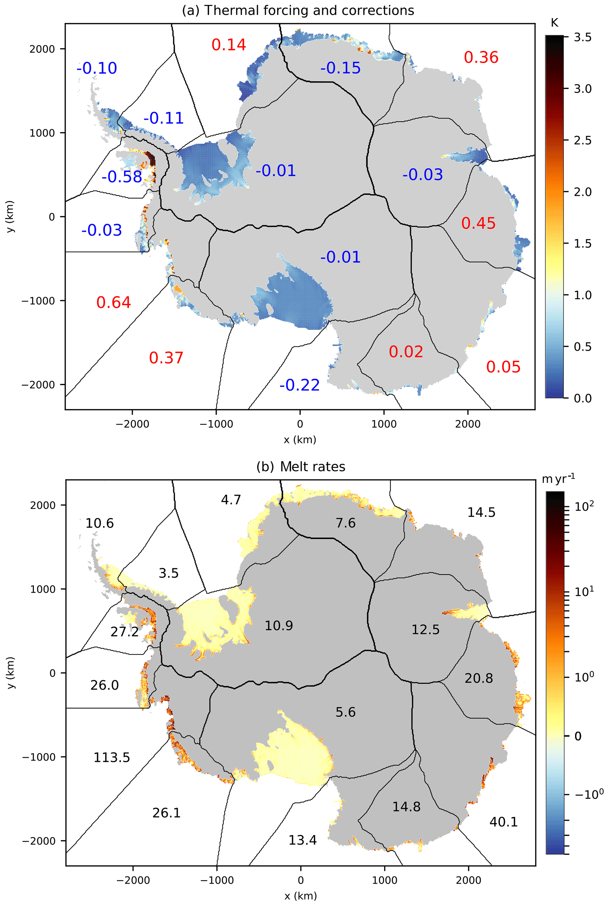
Figure 12 (a) Thermal forcing (shaded) and its corrections (blue and red numbers indicating negative and positive δT, respectively) applied to each sector for nonlocal MeanAnt with a slope dependency (Eq. 1 multiplied by sin θ). (b) Present-day melt rates for nonlocal MeanAnt with a slope dependency. Black numbers indicate melt maxima in individual sectors.

Figure 13 Same as Fig. 10 but using a slope dependency (Eq. 1 multiplied by sin θ).

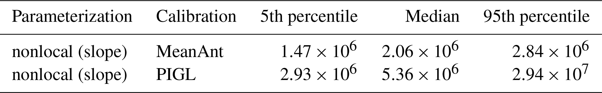
The simple approach of this paper was chosen to facilitate implementation in the wide range of ice sheet models participating in ISMIP6. More complex formulations (e.g., Reese et al., 2018a; Lazeroms et al., 2018; Pelle et al., 2019) involve calculating distances and ice draft slopes, which may not be straightforward for all groups given the short time constraints of ISMIP6 and IPCC-AR6. However, using parameterizations that were derived from analytical physical expressions (e.g., Lazeroms et al., 2019) would make them less dependent on empirical calibration methods and should therefore be encouraged for future ice sheet projections, although further evaluation will also be required. There are also ways to slightly increase the complexity of our approach, for example by including a dependency on the local slope in our simple formulations (Eq. 1 multiplied by sin θ), as suggested by Little et al. (2009) and Jenkins et al. (2018). Applied to nonlocal MeanAnt, this method produces much more realistic melt rates near grounding lines (Fig. 12b), with smaller thermal forcing corrections (Fig. 12a) than without slope dependency (Fig. 5). Introducing the slope dependency also strongly reduces differences between the two calibration methods (Table 3), thereby reducing uncertainty in projected melt rates (Fig. 13). Interestingly, the ice shelf basal mass loss from the slope-dependent version of PIGL is generally significantly lower than from the standard PIGL method (Fig. 13). This parameterization would nonetheless need to be evaluated through an ice sheet model in a similar way as Favier et al. (2019) to make sure that the slope dependency does not produce unstable behaviors and that the temperature dependency is well represented. While we encourage testing this parameterization, it is not part of the ISMIP6 standard protocol.

Table 3 Calibrated γ₀ values (m yr⁻¹) for the quadratic nonlocal parameterization including a dependency on the local slope (Eq. 1 multiplied by sin θ).

The assessment of basal melting parameterizations is strongly limited by the lack of observational temperature and salinity profiles as well as meltwater fluxes at interannual and decadal timescales. The only places where such assessment is possible are the Pine Island and Dotson ice shelves. We have shown that the proposed parameterizations reproduce the general behavior of interannual melt variations for Dotson but not for Pine Island. The calibration method based on the highest melt rates near Pine Island's grounding line (PIGL) produces a range of melt values closer to observational estimates than the alternative method (MeanAnt). Nonetheless, such an assessment remains limited to small, warm cavities. In contrast, the MeanAnt parameters give melt rates that are in better agreement with FESOM ice shelf–ocean projections, at least for Ronne–Filchner. Large present-day biases for warm cavities in FESOM make it useless to assess projections in these environments. It should also be noted that cavity-averaged melt rates are not what ice sheet models are most sensitive to, and melt rates near grounding lines are more relevant (e.g., Reese et al., 2018b).

Beyond the parameterization itself, another limitation of the ISMIP6 ocean forcing is the use of CMIP models to provide the regional ocean warming signal. Indeed, the CMIP models have important biases in the Southern Ocean region in terms of sea ice cover (Turner et al., 2013), westerly winds (Bracegirdle et al., 2013), and ocean temperatures (Little and Urban, 2016; Barthel et al., 2020). These biases likely affect the ice shelf melt projections, even if our anomaly approach is expected to remove a part of the mean-state biases. There are also structural errors in the CMIP models, notably their coarse resolution, which prevents representation of important processes on the Antarctic continental shelf, and the absence of feedbacks between freshwater released through ice shelf and iceberg melting and the ocean components of CMIP models. Recent studies have suggested that the ocean subsurface may warm by a few tenths of a degree by 2100 in response to large freshwater released by the Antarctic Ice Sheet (Bronselaer et al., 2018; Golledge et al., 2019; Schloesser et al., 2019). There are also more local feedbacks that are not represented in our framework. For example, increased ice shelf melting can lead to more advection of offshore circumpolar deep water towards the grounding lines and thereby create a positive feedback to melt rates (Hellmer et al., 2017; Timmermann and Goeller, 2017; Donat-Magnin et al., 2017).

All these feedbacks and the difficulty in parameterizing melt rates clearly point towards ice sheet–ocean coupling as the best way forward for centennial simulations such as ISMIP6. Ideally, ice sheet models would be embedded in the ocean–atmosphere coupled system. However, resolving the ocean circulation in ice shelf cavities at the resolution required to capture all these processes is costly and so far not possible for millennial or large-ensemble simulations. Hence, parameterizations will remain critical, and more work will be needed to assess (i) their ability to reproduce observed melt patterns, (ii) their sensitivity to changing ocean temperature, and (iii) their sensitivity to changing ice draft (slope, size).