the Creative Commons Attribution 4.0 License.
the Creative Commons Attribution 4.0 License.
 | 17 Sep 2020
The future sea-level contribution of the Greenland ice sheet: a multi-model ensemble study of ISMIP6
Sophie Nowicki
Anthony Payne
Eric Larour
Helene Seroussi
William H. Lipscomb
Jonathan Gregory
Ayako Abe-Ouchi
Andrew Shepherd
Erika Simon
Cécile Agosta
Patrick Alexander
Andy Aschwanden
Alice Barthel
Reinhard Calov
Christopher Chambers
Youngmin Choi
Joshua Cuzzone
Christophe Dumas
Tamsin Edwards
Denis Felikson
Xavier Fettweis
Nicholas R. Golledge
Ralf Greve
Angelika Humbert
Philippe Huybrechts
Sebastien Le clec'h
Victoria Lee
Gunter Leguy
Chris Little
Daniel P. Lowry
Mathieu Morlighem
Isabel Nias
Aurelien Quiquet
Martin Rückamp
Nicole-Jeanne Schlegel
Donald A. Slater
Robin S. Smith
Fiamma Straneo
Lev Tarasov
Roderik van de Wal
Michiel van den Broeke
The Greenland ice sheet is one of the largest contributors to global mean sea-level rise today and is expected to continue to lose mass as the Arctic continues to warm. The two predominant mass loss mechanisms are increased surface meltwater run-off and mass loss associated with the retreat of marine-terminating outlet glaciers. In this paper we use a large ensemble of Greenland ice sheet models forced by output from a representative subset of the Coupled Model Intercomparison Project (CMIP5) global climate models to project ice sheet changes and sea-level rise contributions over the 21st century. The simulations are part of the Ice Sheet Model Intercomparison Project for CMIP6 (ISMIP6). We estimate the sea-level contribution together with uncertainties due to future climate forcing, ice sheet model formulations and ocean forcing for the two greenhouse gas concentration scenarios RCP8.5 and RCP2.6. The results indicate that the Greenland ice sheet will continue to lose mass in both scenarios until 2100, with contributions of 90±50 and 32±17 mm to sea-level rise for RCP8.5 and RCP2.6, respectively. The largest mass loss is expected from the south-west of Greenland, which is governed by surface mass balance changes, continuing what is already observed today. Because the contributions are calculated against an unforced control experiment, these numbers do not include any committed mass loss, i.e. mass loss that would occur over the coming century if the climate forcing remained constant. Under RCP8.5 forcing, ice sheet model uncertainty explains an ensemble spread of 40 mm, while climate model uncertainty and ocean forcing uncertainty account for a spread of 36 and 19 mm, respectively. Apart from those formally derived uncertainty ranges, the largest gap in our knowledge is about the physical understanding and implementation of the calving process, i.e. the interaction of the ice sheet with the ocean.
- Article
(5166 KB) - Full-text XML
-
Supplement
(22408 KB) - BibTeX
- EndNote


The aim of this paper is to estimate the contribution of the Greenland ice sheet (GrIS) to future sea-level rise until 2100 and the uncertainties associated with such projections. The work builds on a worldwide community effort of ice sheet modelling groups that are organized in the framework of the Ice Sheet Model Intercomparison Project for CMIP6 (ISMIP6), which is endorsed by the Coupled Model Intercomparison Project (CMIP6). This is the first time that process-based projections of the ice sheet sea-level contribution are systematically organized for the entire global ice sheet modelling community, extending earlier initiatives that were separated between the USA (SeaRISE, http://websrv.cs.umt.edu/isis/index.php/SeaRISE_Assessment, last access: 15 August 2020) and Europe (ice2sea, https://www.ice2sea.eu, last access: 15 August 2020). In addition to the actual projections, the less tangible but equally important achievement of ISMIP6 is the building of a community and the creation and design of an intercomparison infrastructure that has not existed before. The link with CMIP illustrates the ambition to bring community ice sheet model projections to the level of existing initiatives, e.g. in the field of coupled climate model simulations (Eyring et al., 2016). The project output and timeline are oriented towards providing input for the sixth assessment cycle of the Intergovernmental Panel on Climate Change (IPCC), where earlier assessments (Church et al., 2013; Oppenheimer et al., 2019) had to rely on input from various sources to provide ice sheet sea-level change projections. The present results are complemented by another paper on Antarctic ice sheet projections (Seroussi et al., 2020).
The overall mass balance of the GrIS is governed by the surface mass balance (SMB) that determines the amount of mass that is added by snow accumulation and removed by meltwater run-off and sublimation and by the amount of mass that is lost through a large number of marine-terminating outlet glaciers. Over the period 1992–2018, the ice sheet has lost mass at an average rate of ∼ 140 Gt yr−1, which is equivalent to a sea-level contribution of ∼ 0.4 mm yr−1 (The IMBIE Team, 2019). The contribution of SMB-related changes to these figures is ∼ 52 %, with the remaining 48 % being due to increased discharge of outlet glaciers (The IMBIE Team, 2019).
Process-based future ice sheet projections rely on numerical models that simulate the gravity-driven flow of ice under a given environmental forcing, subject to boundary conditions at the surface, base and at the lateral boundaries. In our stand-alone modelling approach that connects to CMIP, the atmospheric and oceanic forcing is derived from CMIP Global Climate Model (GCM) output.
This work continues from an earlier ISMIP6 project (initMIP-Greenland; Goelzer et al., 2018) that compared the initialization techniques used by different ice sheet modelling groups. In many cases, the ice sheet projections presented here are directly based on modelling work that entered that earlier comparison. Differences between ice sheet models and, in particular, different ways of using the models are a large source of uncertainty (Goelzer et al., 2018). The specific contribution of the present analysis to the range of existing future sea-level change projections lies therefore in the quantification of ice sheet model (ISM) uncertainty, which is done here for the first time in a consistent framework.
In the following we discuss the approach and experimental set-up in Sect. 2 and briefly present the participating models in Sect. 3. We analyse the modelled initial state (Sect. 4.1), the 21st-century projections (Sect. 4.2) and associated uncertainties (Sect. 4.3) and close with a discussion and conclusions (Sect. 5). The two appendices give more detailed information about the participating models (Appendix A) and list the model results (Appendix B).
In this section we describe the approach and experimental set-up for GrIS sea-level change projections performed within the framework of ISMIP6. While focused on the scientific aims described in the introduction, the experimental framework is designed to be inclusive to a wide number of modelling approaches. We allow modelling groups to participate with more than one submission to explore modelling choices like different horizontal grid resolution or initialization techniques with the same model. We also accommodate models from the same code base but used by different groups, knowing that modelling decisions (e.g. the chosen initialization strategy) can be more important for the results than the underlying numerical scheme. The result is a heterogeneous set of ice sheet models that can be understood as an ensemble of opportunity. In the following we refer to each of the 21 individual submissions as a “model”, encompassing the code base as well as the modelling decisions (parameter choices, applied approximations, initialization strategy).
The experimental design of ISMIP6-Greenland projections extends the protocol of earlier ISMIP6 initiatives (Nowicki et al., 2016; Goelzer et al., 2018; Seroussi et al., 2019) and is described in detail in a separate publication (Nowicki et al., 2020). Here we only summarize the most important aspects and refer to detailed descriptions elsewhere. The actual ice sheet projections for the period 1 January 2015–31 December 2100 are tightly defined in terms of forcing and how to apply it, while the preceding ice sheet initialization and historical run are largely up to the individual modeller.
Ice sheet model (ISM) initialization to the present-day state is a critical aspect of any future ice sheet projection (Goelzer et al., 2017, 2018). It consists of defining the prognostic model state with the overall aim here to represent the present-day dynamic state of the GrIS as well as possible. In some cases modellers may initialize to a recent state of the ice sheet during the satellite era for which a large number of detailed observations of velocity and ice thickness are available. In other cases, the models may be initialized using spin-up techniques or steady-state assumptions at some earlier stage of the ice sheet history or hybrid approaches that combine features of optimization and spin-up (e.g. Pollard and DeConto, 2012). See Goelzer et al. (2017, 2018) for a comparison and an overview of different initialization strategies currently used in the ice sheet modelling community.
The experimental set-up of the initialization and the historical experiment leading up to the projections is left free to be decided by the modellers (see Appendix A). The only requirement is that the model state at the end of the historical run should represent the state of the GrIS at the end of 2014 as a starting point for future projections. This time frame is set by CMIP6 requirements (Eyring et al., 2016). The length of the historical runs will consequently differ based on the initialization strategy of each individual model.
Being an officially endorsed sub-project of CMIP6, the experimental design of ISMIP6 projections builds heavily on output of CMIP GCMs that are used to produce the forcing for ice sheet models over the 21st century. While ISMIP6 has proposed ice sheet model projections based on CMIP6 GCM output as part of its extended experimental design (Nowicki et al., 2020), the results discussed in this paper focus solely on CMIP5-based forcing. Working with CMIP5 output has allowed us to select GCMs from a well-defined ensemble and sample the CMIP5 ensemble range in a controlled way, while CMIP6 model results are still being produced. For the core experiments that are the main focus of this paper, we have selected three CMIP5 GCMs that perform well over the historical period and maximize the spread in future projections of a number of key climate change metrics relevant for GrIS evolution (Barthel et al., 2020). Three additional CMIP5 GCMs were selected using the same principle to extend the ensemble. We use the two scenarios RCP8.5 and RCP2.6 to cover a wide range of possible future climate evolution scenarios with particular focus on RCP8.5 (see Table 1). Exploring other scenarios was deprioritized in favour of a feasible workload for the ice sheet modellers and for producing forcing data.
Table 1List of GCM-forced experiments for ISMIP-Greenland projections. Climate model uncertainty is sampled with three core GCMs and three additional extended GCMs. Two different scenarios (RCP8.5, RCP2.6) are evaluated for model MIROC5. Sensitivity to the ocean forcing is sampled with three experiments under scenario RCP8.5. Forcing for the historical experiment is defined by each individual modeller (not shown). Experiment “ctrl_proj” applies zero SMB anomalies, no SMB-height feedback and a fixed retreat mask (not shown).

* Experiments exp01–exp04 are open-framework experiments not listed here with the same GCM forcing as exp05–exp08. See text for details.
The GCM output is used to separately derive ice sheet model forcing for the interaction with the atmosphere and the ocean.
Interaction with the atmosphere is incorporated in the models by prescribing surface mass balance (and temperature) anomalies relative to the period 1960–1989, for which the ice sheet is assumed to be in balance with the forcing (e.g. Mouginot et al., 2019). The forcing is produced with the regional climate model MAR version v3.9 (Fettweis et al., 2013, 2017) that locally downscales the GCM forcing to the GrIS surface (Fig. 1a, b). We take into account changes in the SMB due to elevation changes using a parameterization based on MAR output for the same simulation (Nowicki et al., 2020). In cases where the modelled initial ice sheet differs substantially from the observed, we remap the SMB anomalies from the observed geometry to the modelled geometry using a technique developed specifically for that purpose (Goelzer et al., 2020b).
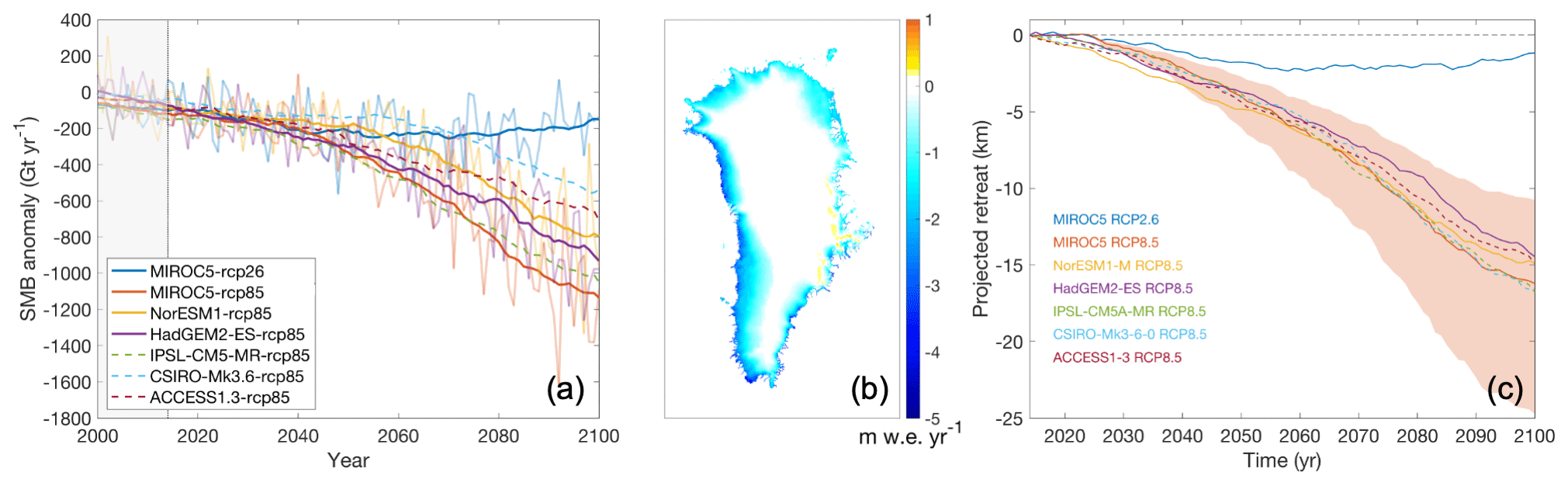
Figure 1Illustration of atmospheric and oceanic forcing. (a) Greenland-wide SMB anomaly for projections starting at 2015. Strong lines are 10-year running mean values for the core experiments (solid) and extended CMIP5 experiments (dashed), plotted over the full time series in the background (omitted for the extended experiments for clarity). (b) spatial pattern of the average MIROC5-RCP8.5 SMB anomaly for the period 2091–2100. (c) Greenland-wide average of prescribed tidewater glacier retreat (Slater et al., 2019, 2020). The shading gives the range of ocean sensitivity sampled with two more experiments in MIROC5-RCP8.5-high and MIROC5-RCP8.5-low.
The standard approach for ocean forcing is based on an empirically derived retreat parameterization for tidewater glaciers (Slater et al., 2019, 2020) that is forced by MAR run-off and ocean temperature changes in seven drainage basins around Greenland. The forcing is illustrated as Greenland-wide average of prescribed tidewater glacier retreat in Fig. 1c. In this retreat implementation, retreat and advance of marine-terminating outlet glaciers in the ISMs are prescribed as a yearly series of maximum ice front positions (Nowicki et al., 2020). This approach is a strong simplification of the complex interaction between marine-terminating outlet glaciers and the ocean, for which physically based solutions are in development but not available for all models. The retreat parameterization is designed to be used in the wide variety of models under consideration. Uncertainty in the parameterization is translated into a set of three ocean sensitivities (medium, high, low) covering the median, 75 % and 25 % percentiles of sensitivity parameter κ that controls the amount of retreat given ocean temperature change and ice sheet run-off (Slater et al., 2019, 2020). Results are explored with the last two core experiments (Table 3).
For some ISMs of high spatial resolution that incorporate a physical calving model, future evolution of marine-terminating outlet glacier is alternatively forced directly by changes in ocean temperature and run-off derived from the GCM and Regional Climate Model (RCM) output (Slater et al., 2020). Simulations performed with this submarine melt implementation are considered as a contribution to the open framework of the exercise, designed to allow exploration of novel modelling techniques that cannot be implemented in all models. We have decided to include model results from this open framework in our main analysis since they represent a source of additional uncertainty in the way the forcing is applied. For this group of models, the last two experiments that sample uncertainty due to ocean forcing are not defined (Table 3).
Model output for the ISMIP6 experiments is initially produced by the participating groups on the individual native grid of their models, then conservatively interpolated to a standard regular grid with a resolution close to the native grid for submission to our archive and finally conservatively interpolated to a common 5 km×5 km regular diagnostic grid for analysis. In a few models, the native grid is identical to the diagnostic grid. All results presented in this paper are based on data on the common diagnostic grid.
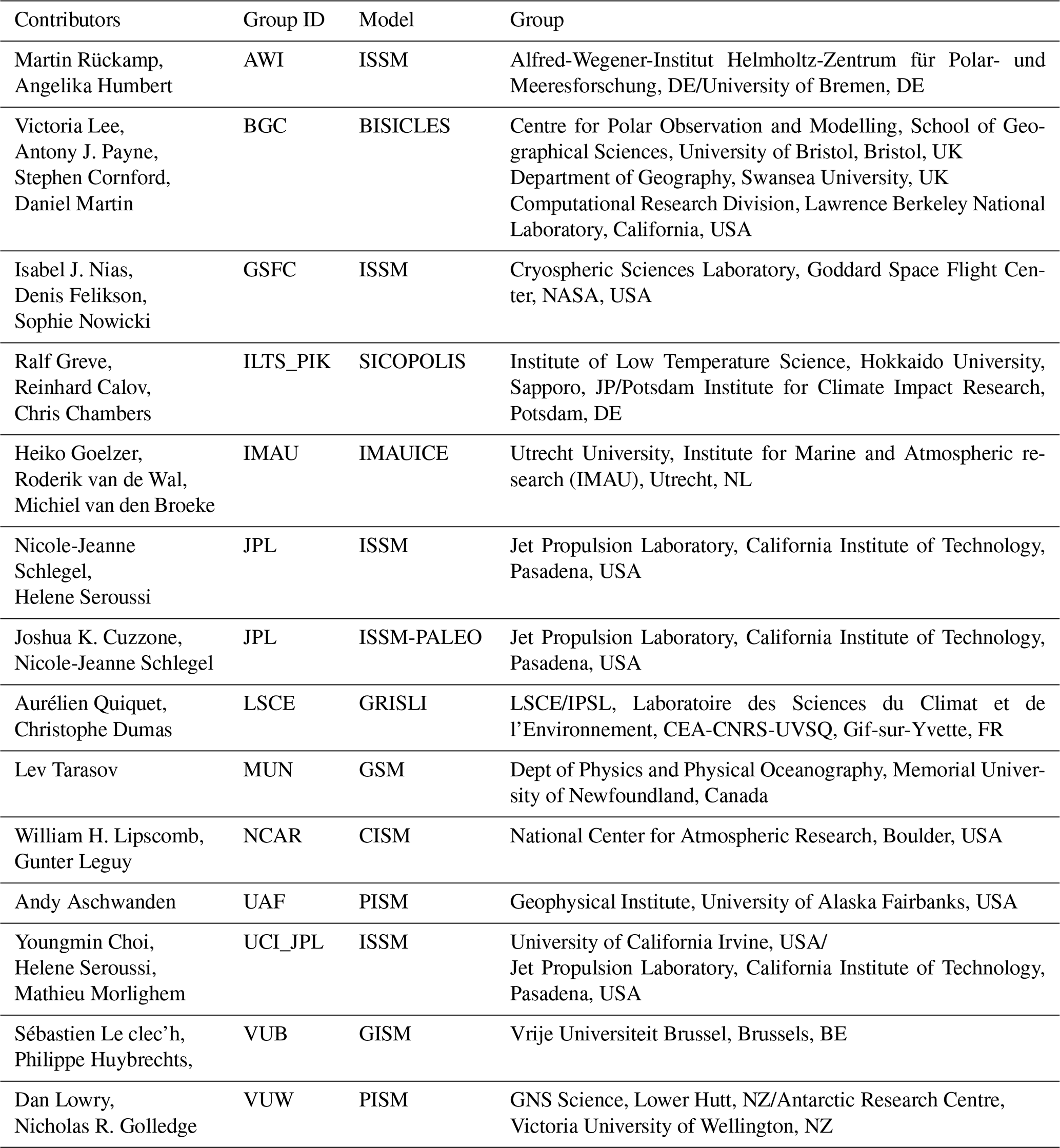
Table 2Participants, modelling groups and ice sheet models in ISMIP6-Greenland projections.
One of the main results presented below is the projected sea-level contribution of the GrIS to 21st-century sea-level rise. In all cases, we calculate sea-level changes based on the evolving ice sheet geometry, taking into account the model specific densities for ice and sea water and correcting for the map projection error following Goelzer et al. (2020a). In agreement with the GlacierMIP exercise (http://www.climate-cryosphere.org/mips/glaciermip/about-glaciermip, last access: 15 August 2020), we have attempted to remove the contribution of loosely connected glaciers and ice caps in the periphery of Greenland from our mass change estimates to avoid double-counting in global sea-level change assessments. This has been done by correcting the ice sheet mass change per grid cell by the area fraction of the glaciers (level 0–1) in the Randolph Glacier Inventory (RGI Consortium, 2017). The assumed constant ocean area for conversion from ice mass above flotation to sea-level equivalent (SLE) is 3.625×10¹⁴ m2 (Cogley, 2012; Gregory et al., 2019), which implies that 1 mm SLE equals 362.5 Gt ice mass. For cases where the model simulates isostatic adjustment, we have assumed that corrections of the ice mass above flotation due to bedrock changes are negligible on the centennial timescale (Goelzer et al., 2020a). All sea-level contributions are corrected for model drift by subtracting the sea-level contribution from a control experiment (ctrl_proj) and are therefore relative to the year 2014. This correction implies that the reported numbers have to be interpreted as the ice sheet response to future forcing in addition to a background evolution that arises from forcing before 2014, sometimes called the committed sea-level contribution (e.g. Price et al., 2011). This committed contribution is expected to be positive for Greenland but much lower than the observed trend before 2014 (The IMBIE team, 2019) because the mass loss rate rapidly decreases in absence of additional forcing (Price et al., 2011). For ensemble statistics we report mean (μ) and the 2× standard deviation (2σ) range to quantify the uncertainty unless stated differently in the text.
We have 21 submissions from 14 modelling groups, covering a wide range of the global ice sheet modelling community (Table 2). Compared to initMIP-Greenland (Goelzer et al., 2018) the number of participating modelling groups has slightly decreased with some removals and some new additions, but the range of represented models is still broad. A detailed description of the individual models and initialization techniques is given in Appendix A together with a table of important model characteristics (Table 4). The total range of horizontal grid resolution is between 0.2 and 30 km, where extreme values come from finite element models with adaptive grid resolution that have high resolution near the margins to resolve narrow outlet glaciers and low resolution inland. All participating models use either a form of data assimilation or nudging techniques of different degrees to improve the match with present-day observations (Table 4).
All groups have contributed a complete set of core experiments (Table 3), which form the basis of the analysis for this paper. The submissions are identified by the group ID and model name (Table 2) and a counter to distinguish several submissions from the same group (Table 3). Four models have used the non-standard open forcing framework (BGC-BISICLES, UAF-PISM2, UCIJPL-ISSM2, VUW-PISM), which does not define the ocean sensitivity experiments exp09 and exp10. In the BGC-BISICLES case, they have been replaced by their own interpretation of high and low ocean forcing. The two models MUN-GSM1 and MUN-GSM2 have used remapped SMB anomalies (Goelzer et al., 2020b) to optimize the forcing for their initial geometry, which differs more from the observations compared to other models.
Table 3Experiment overview. List of experiments that have been performed by the participating groups.
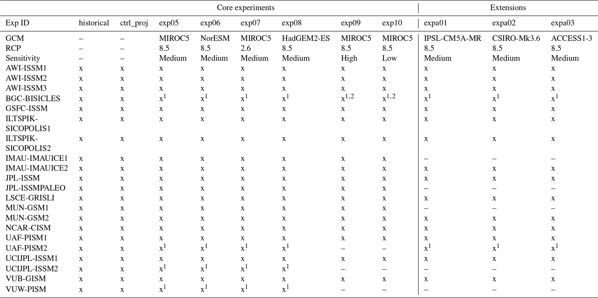
1 Open format not using the retreat parameterization. 2 Own strategy to produce high and low ocean forcing.
In this section we first present ice sheet modelling results for the end of the historical run, forming the starting point of sea-level change projections over the 21st century. This is followed by the results of the projections, with a focus on the GrIS sea-level contribution and associated uncertainties.
4.1 Historical run and initial state
The initial model states at the end of 2014 differ among the models in the ensemble as a result of different initialization strategies, forcing and parameter choices. Figure 2 illustrates the diversity of modelled initial ice sheet area by showing the sum of grounded ice coverage across the ensemble. Disagreement in the periphery is partially related to a choice left deliberately to the individual modellers: which part of the ice-covered area of Greenland should be modelled. While some modellers target the entire observed ice-covered area, others mask out unconnected or loosely connected glaciers, ice caps and ice fields in an attempt to avoid double-counting of those features in global assessments (see modelled ice masks for individual models in Fig. S4 in the Supplement).
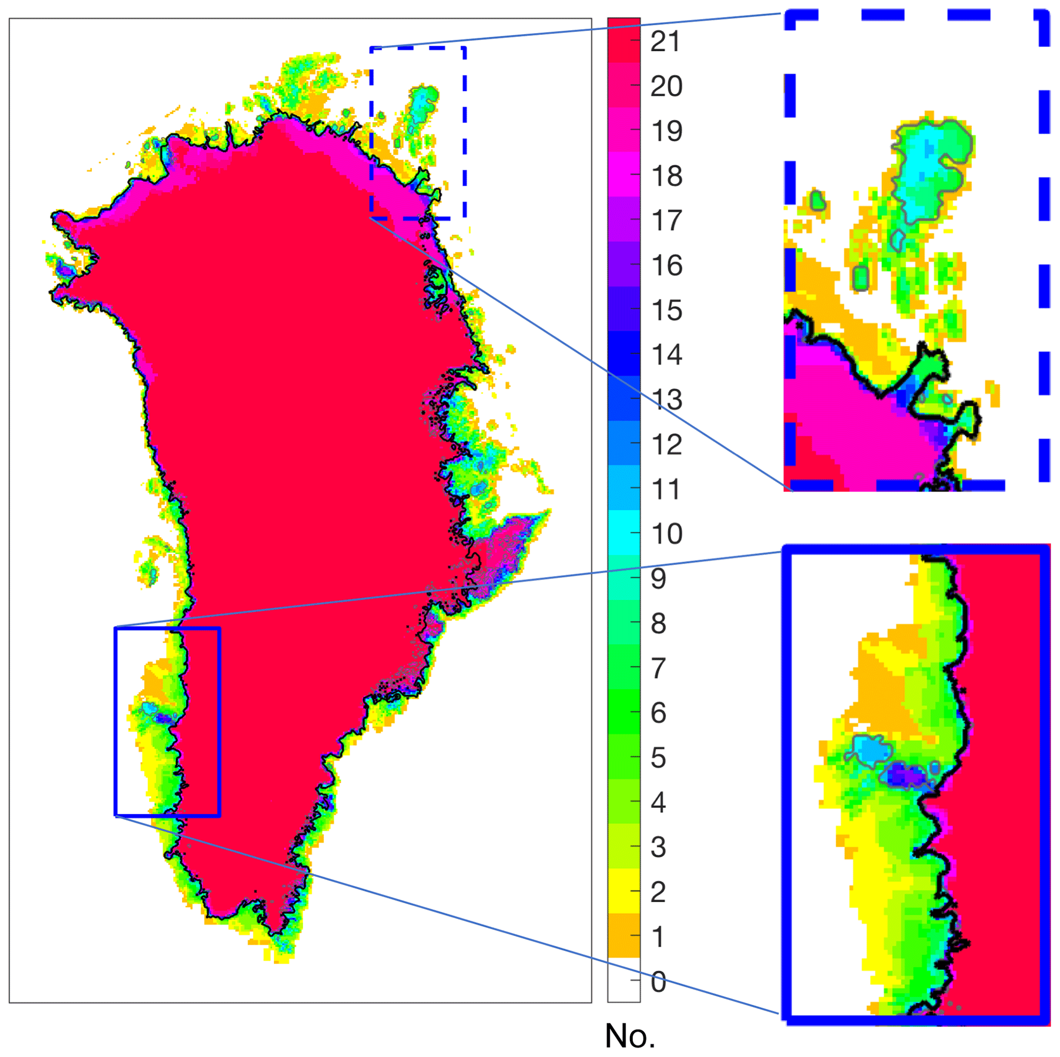
Figure 2Common initial ice mask of the ensemble of models in the intercomparison. The colour code indicates the number of models (out of 21 in total) that simulate ice at a given location. Outlines of the observed main ice sheet (Rastner et al., 2012) and all ice-covered regions (i.e. main ice sheet plus small ice caps and glaciers; Morlighem et al., 2017) are given as black and grey contour lines, respectively. A complete set of figures displaying individual model results is given in the Supplement.
Another view on the model spread for the initial state can be seen in Fig. 3, which shows the grounded ice area and grounded volume for all models in the ensemble. In comparison we show two different observed values that equally depend on the choice of which part of the ice-covered area to include in the estimate. This notably leads to a large range in area between a low estimate (main ice sheet; Rastner et al., 2012) and high estimate (all ice-covered area; Morlighem et al., 2017), while the volume difference is relatively small due to the limited thickness of peripheral glaciated areas. Compared to initMIP-Greenland (cf. Fig. 2 in Goelzer et al., 2018, but note the different-coloured map), the spread in initial states has been considerably reduced, which is partially related to ongoing improvements of the modelling techniques of individual groups and partly because some extreme models are not part of the ensemble anymore.
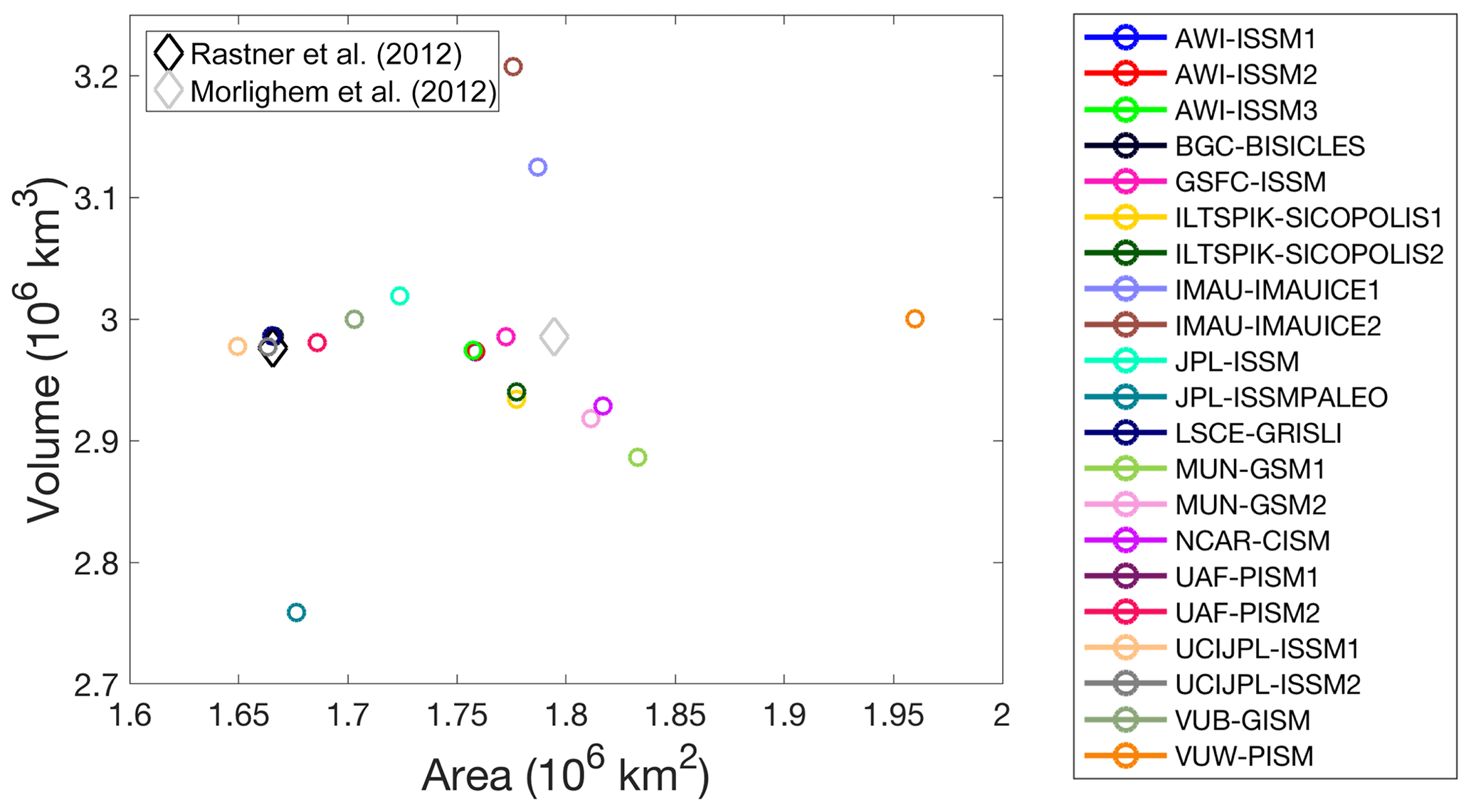
Figure 3Grounded ice area and grounded volume for all models (circles). Observed values (Morlighem et al., 2017) are given for the entire ice-covered region (light-grey diamond) and for the region of the main ice sheet (black diamond) where loosely connected glaciers and ice caps are removed (Rastner et al., 2012).
The initial model state at the end of 2014 is the result of a model-specific initialization that includes a short historical run. We display the ice mass evolution for this experiment followed by a standardized control experiment (ctrl_proj) for the same period as the projections but assuming zero SMB anomalies and a fixed retreat mask from 2015 onwards (Fig. 4). In most models the ice sheet experiences a mass loss during the historical period, but the magnitude often falls below the observed range. In some cases this discrepancy is explained by the fact that the ice sheet is exposed to GCM forcing over the historical period which does not exhibit the observed interannual and interdecadal variability. In other cases, the historical run is not specifically forced, rather representing the background evolution arising as an artefact of the initialization. In any case, representing the historical mass loss accurately was not a strong priority for our experimental set-up, where any background evolution is effectively removed by subtracting results of experiment ctrl_proj.
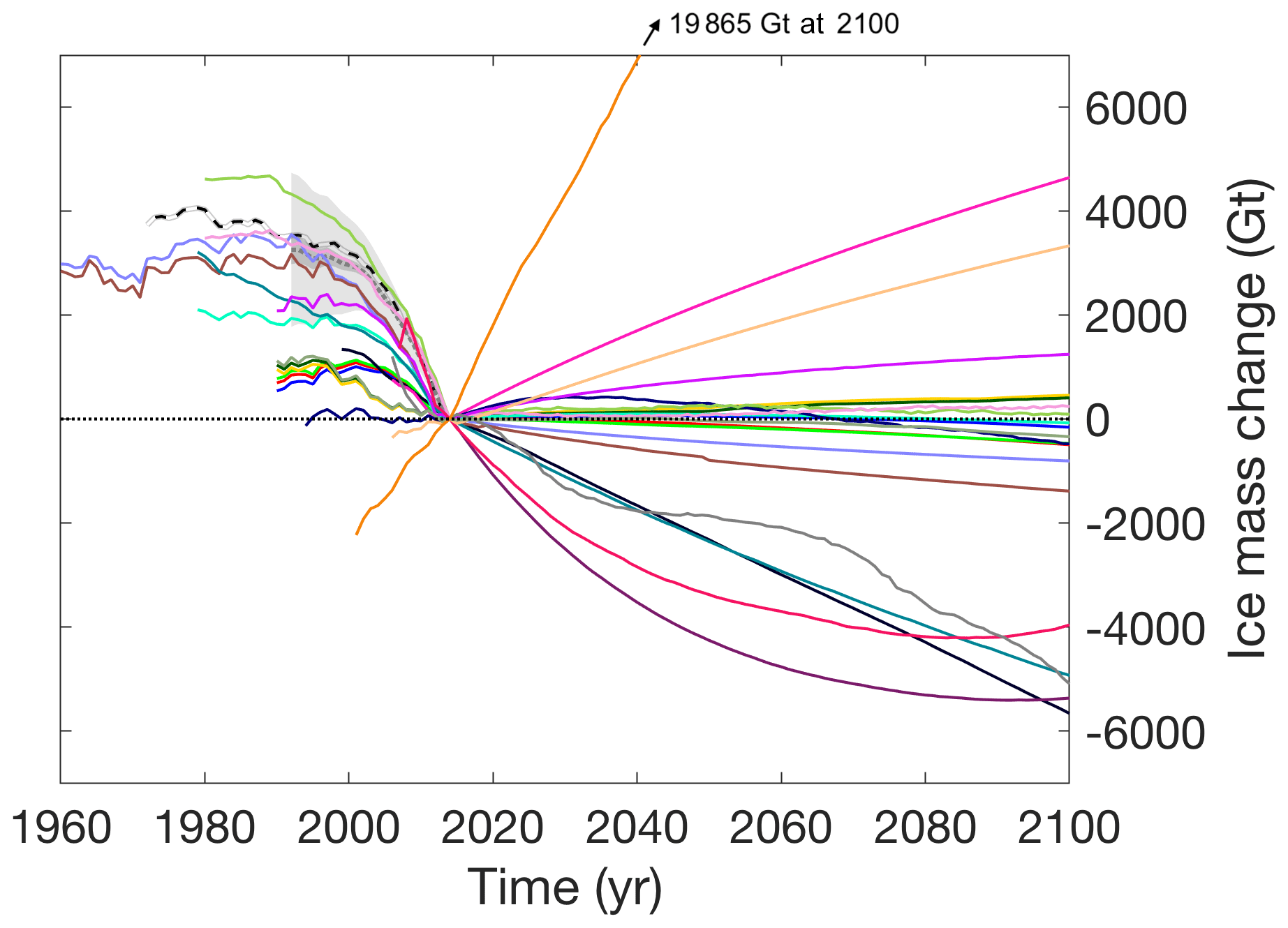
Figure 4Ice mass change relative to the year 2014 for the historical run and experiment ctrl_proj. The colour scheme is the same as in Fig. 3. Recent reconstructions of historical mass change (The IMBIE Team, 2019) are given as a dotted grey line with cumulated uncertainties assuming fully correlated and uncorrelated errors in light and dark shading, respectively. The dashed black-and-white line shows one specific reconstruction going back longer in time (Mouginot et al., 2019).
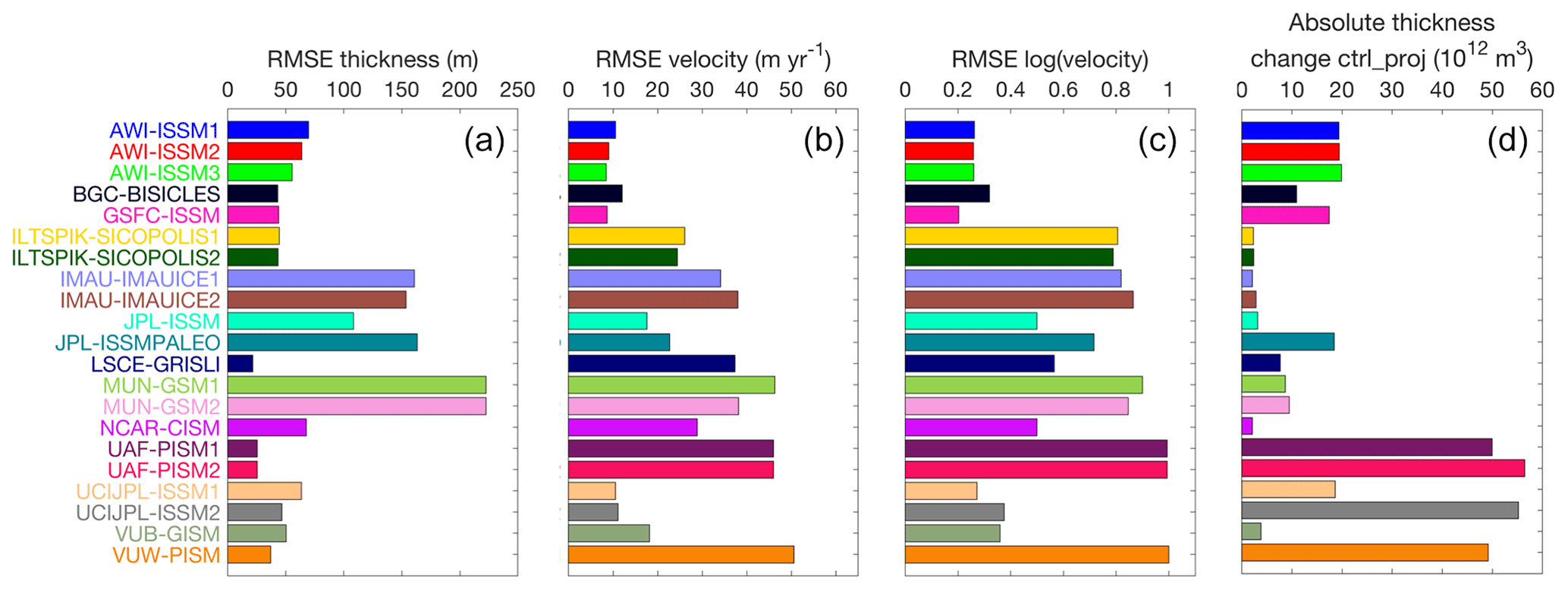
Figure 5(a–c) Error estimate of model output at the end of the historical run compared to observations. (a) Root mean square error (RMSE) of ice thickness compared to observations (Morlighem et al., 2017). RMSE of the horizontal velocity magnitude (b) and the logarithm of the horizontal velocity magnitude (c) compared to observations (Joughin et al., 2016). The diagnostics have been calculated for grid cells subsampled regularly in space to reduce spatial correlation; we show median values for different possible offsets of this sampling. (d) Absolute thickness change in experiment ctrl_proj integrated over the model grid.
The control experiment (ctrl_proj) is in most cases the result of competing tendencies to (1) continue the mass trend before 2014 and (2) relax toward an unforced state as a result of removing the anomalies at the start of the projection period in 2015. The ensemble range of sea-level contribution due to that drift in experiment ctrl_proj is −50 to 15 mm (Table B1).
We further evaluate the initial model state at the end of 2014 in comparison to ice-sheet-wide observational datasets (Fig. 5). We calculate the root mean square error (RMSE) of the modelled data compared to observations of ice thickness (Morlighem et al., 2017) and horizontal surface velocity magnitude (Joughin et al., 2016). The diagnostics are calculated for subsampled data to reduce spatial correlation in the error estimates, and we show median values for different offsets. The comparison shows a wide diversity of the models in terms of their match with the observed ice thickness distribution (Fig. 5a) and velocity (Fig. 5b). We include a comparison with the logarithm of the velocity magnitude (normalized by 1 m yr−1), which reduces the emphasis of errors in high velocities at the margins (Fig. 5c). These diagnostics are complemented by the absolute ice thickness change in ctrl_proj that serves as a measure of the model drift (Fig. 5d). The largest thickness errors arise for coarse-resolution models that show substantial mismatches in particular at (but not limited to) the ice sheet margins. These are also models that do not apply calibration techniques to optimize the geometry during initialization. Some of the models with the lowest RMSE for ice thickness (e.g. LSCE-GRISLI and UAF-PISM) show relatively large errors in velocity, indicative of the prioritized field during optimization (thickness) and of the dependence between geometry and dynamic behaviour. Nevertheless, a few examples show that low errors in thickness and velocity are not mutually exclusive. See Figs. S3, S4 and S5 for a visual comparison of individual models with observations for ice thickness, surface elevation and velocity, respectively.
While a formal ranking and weighting of the ice sheet models based on the provided information is outside of the scope of this paper, we caution that different evaluation metrics should be combined and balanced in that case. This has already been mentioned for the comparison of errors in ice thickness and velocity. Another example is that good agreement of the ice sheet model geometry or surface velocity with observations can go hand in hand with a large drift in the control experiment (Fig. 5d), which may indicate too short of a relaxation during initialization. Similarly, modifying the applied background SMB forcing can be used to reduce mismatch with the observed velocity and geometry. Finally, masking operations can be used to constrain the ice sheet model area and consequently the geometry, reducing the prognostic capabilities of the model. Combining complementary metrics and auxiliary information should be used in model ranking and weighting attempts. Another aspect that would have to be carefully considered for model weighting for ensemble statistics is the fact that several models have strong similarities and their results may therefore be overrepresented in the ensemble.
4.2 Projections
In the following we first present sea-level projections for the four core experiments with medium ocean forcing sensitivity. Results of the projection experiments (2015–2100) are always presented relative to a control experiment (ctrl_proj) with a focus on MIROC5-forced experiments, which shows the strongest warming among the three selected GCMs. The ensemble mean ice thickness changes for scenario MIROC5-RCP8.5 shows a strong thinning at the margin due to the effect of increased surface meltwater run-off and marine-terminated glacier retreat (Fig. 6a). The strongest response is seen at the marine margins where both effects combine to a thinning of up to several hundred metres, while the interior of the ice sheet is thickening less than 10 m in response to increased snow accumulation, except for some places in the south-east, where the thickening can reach 20 m and more.
The spread in the projections due to ice sheet model uncertainty and its spatial distribution is illustrated in Fig. 6b, showing the ensemble standard deviation for experiment MIROC5-RCP8.5. The regions of largest uncertainty overlap with the regions of largest thinning due to differences in the response of tidewater glaciers and their precise location in different models. The response to the anomalous SMB forcing is more homogeneous between models (cf. Fig. S8) as the magnitude is largely prescribed and can mostly vary due to differences in ice masks across the ensemble. Exceptions are the remapped SMB anomalies (MUN-GSM1, MUN-GSM2) that are displaced to match the model geometry and height-dependent SMB changes that are model specific, visible in the north-east.
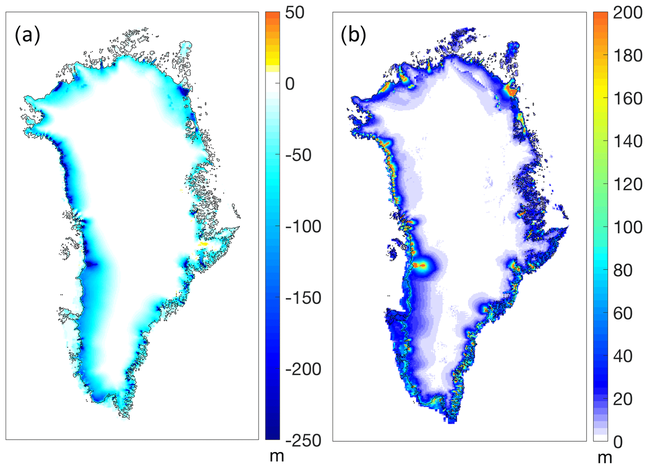
Figure 6Ensemble mean (a) and standard deviation (b) of ice thickness change in MIROC5-RCP8.5 minus control over the 21st century. Thin black lines indicate the observed ice-covered area (Morlighem et al., 2017).
The sea-level contribution for MIROC5-RCP8.5 is steadily increasing in all ice sheet models with an increasing rate of change until the end of the 21st century, indicative of accelerating mass loss for this very high emission scenario (Fig. 7b). Short-term variability in this diagnostic is mainly due to interannual variability in the applied SMB forcing and therefore synchronized across the ensemble. The average rate of change across the ensemble is 0.9 and 2.4 mm yr−1 over the periods 2051–2060 and 2091–2100, respectively.
The total GrIS sea-level contribution by 2100 for MIROC5-RCP8.5 is projected between 67 and 135 mm, with an ensemble mean (n=21) and 2σ range of 101±40 mm. In contrast, GCM MIROC5 forced under scenario RCP2.6 leads to a contribution of only 32±17 mm, and forcing from the two other core GCMs for the RCP8.5 scenario lead to contributions of 83±37 and 69±38 mm for HadGEM2-ES and NorESM1, respectively (Fig. 7a). Detailed results for all models and scenarios are given in Fig. 12 and listed in Table 5 in Appendix B.
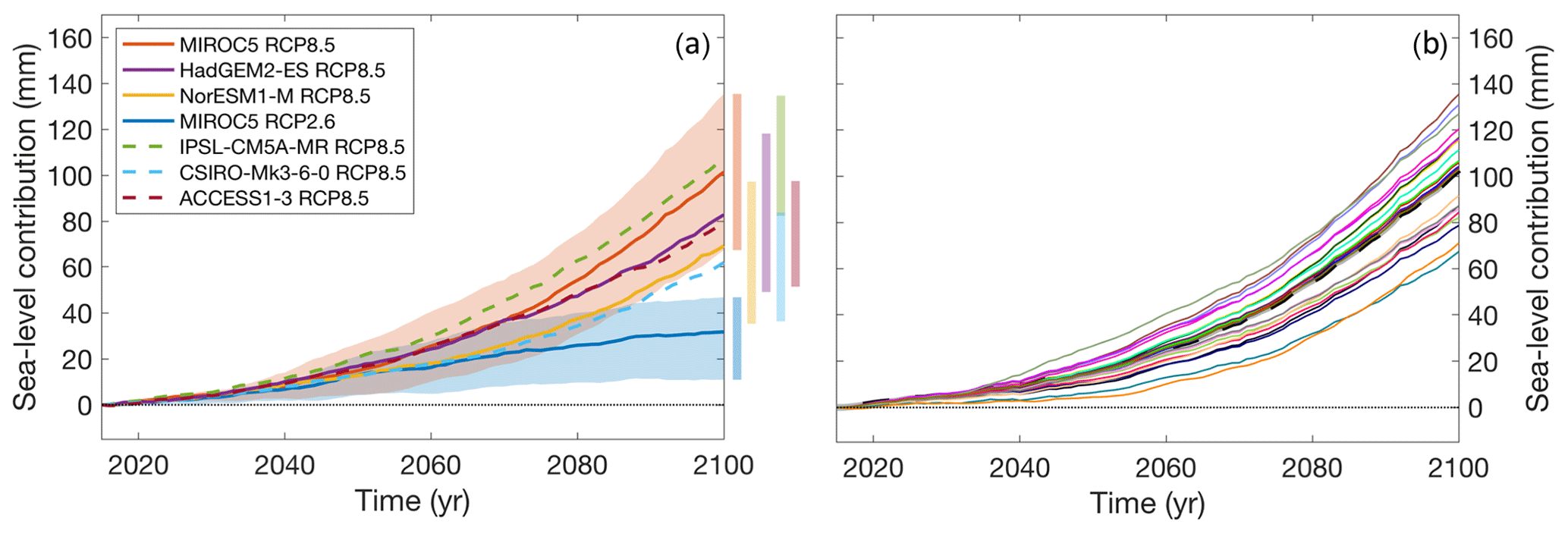
Figure 7Ensemble sea-level projections. (a) ISM ensemble mean projections for the core experiments (solid) and extended experiments (dashed). The background shading gives the model spread for the two MIROC5 scenarios and is omitted for the other GCMs for clarity but indicated by the bars on the right-hand side. (b) Model specific results for MIROC5-RCP8.5. The colour scheme is the same as in previous figures. The dashed line is the result of applying the atmosphere and ocean forcing to the present-day ice sheet without any dynamical response (NOISM).
Differences in results between individual ice sheet models are not easily linked to general ice sheet model characteristics (e.g. resolution, approximation to the force balance, treatment of basal sliding), and the relatively small ensemble size prevents us from applying statistical approaches to do so. Nevertheless, a few notable differences can be mentioned. Models using the open framework overall show lower contributions compared to models using the standard retreat forcing, although they are not clear outliers in the range of projections. Results from the two groups that have applied both approaches in parallel confirm this conclusion (see Table 5). For example, RCP8.5 results from models using the open approach (n=4) are on average 23 mm lower compared to results under standard forcing. Focussing on the latter group (standard forcing), models with larger initial area and volume tend to produce larger sea-level contributions. This is the expected behaviour given the effect of both forcing mechanisms: (1) a model of larger ice sheet extent will produce more run-off at the margins under the anomalous SMB forcing; (2) thicker and more extended marine ice sheet margins will lose more mass to the retreat parameterization.
The end members of the ensemble in terms of sea-level contribution (IMAU-IMAUICE2: high; JPL-ISSMPALEO: low) are amongst the models with the lowest resolution in the ensemble, which could suggest that low-resolution models have larger uncertainty but not necessarily a bias. However, note that the two lowest models (JPL-ISSMPALEO and VUW-PISM) did not apply the SMB-height feedback, which may explain some of the low response for these models.
We can also compare results to a schematic experiment where atmosphere and ocean forcing is applied to the present-day ice sheet without any dynamical response (NOISM, grey dashed line in Fig. 7b). The only exception is the SMB-height feedback that is propagated according to height changes due to the applied SMB anomaly itself and due to local thinning at the margins where the retreat mask is applied. In this approach, biases in the initial state are reduced to measurement uncertainties, while dynamic changes are ignored by construction. If the dynamic response of the ice sheet to the retreat mask forcing is expected to increase the mass loss, one could suggest that for the observed geometry and for a given forcing, NOISM should serve as a lower bound to a “perfect” projection in our standard framework. Because NOISM currently tracks the ensemble mean of the projections, the argument could be extended to suggest that taking the model mean for the best guess could imply a low bias.
We do not have a dedicated core experiment to separate the effect of the parameterized SMB-height feedback from the ensemble of models. But such analysis will be possible with some of the extended experiments that are in preparation. If we were to rely on results of NOISM, the feedback accounts for 6 %–8 % of the total sea-level contribution in the year 2100 for RCP8.5 experiments, confirming similar numbers from earlier studies (Goelzer et al., 2013; Edwards et al., 2014a, b). However, the NOISM figures are subject to small biases due to missing dynamic height changes that would, for example, thin the marine margins and relatively thicken land-terminated ice sheet margins that are steepening in these projections in response to the anomalous SMB forcing.
4.3 Uncertainty analysis
In this section we analyse uncertainties in ice sheet response due to ISM differences, forcing scenarios and GCM boundary conditions on a regional basis. We use an existing basin delineation (IMBIE2-Rignot, Rignot et al., 2011) that separates the ice sheet into six drainage basins, which has been extended outside the observed ice mask to accommodate larger-than-observed ice sheet model configurations (see inset in Fig. 8).
The results in Fig. 8 show the projected contribution to sea-level rise in the year 2100, indicating a north–south gradient with larger contributions from the south. The basin with the largest contributions is “SW” due to an extended ablation zone in south-west Greenland, which is the region with the largest source of sea-level contribution from changes in SMB already observed (The IMBIE Team, 2019; Mouginot et al., 2019). However, note for this comparison that the basins do not all have the same area. When we interpret the ensemble standard deviation relative to the ensemble mean as a measure for ice sheet model uncertainty, the largest uncertainty of ∼ 40 % is present in the “NO” and “SE” basins and the lowest uncertainty of 17 % in the “SW” basin. The good agreement between models for “SW” can be explained by the dominance of the SMB forcing in this basin, which is prescribed in our experiments, so that variations between models mainly occur due to differences in ice sheet mask.
Comparing results for RCP8.5 between the three GCMs side by side (Fig. 8) shows that the SW basin has the lowest ISM interquartile range in all cases but is also one of the two basins (SW and NE) with the largest difference between GCMs. While the large GCM difference in the SW can be explained by the GCM-specific warming pattern and their influence on the SMB forcing, differences in the NE basin are governed mainly by the ocean forcing.
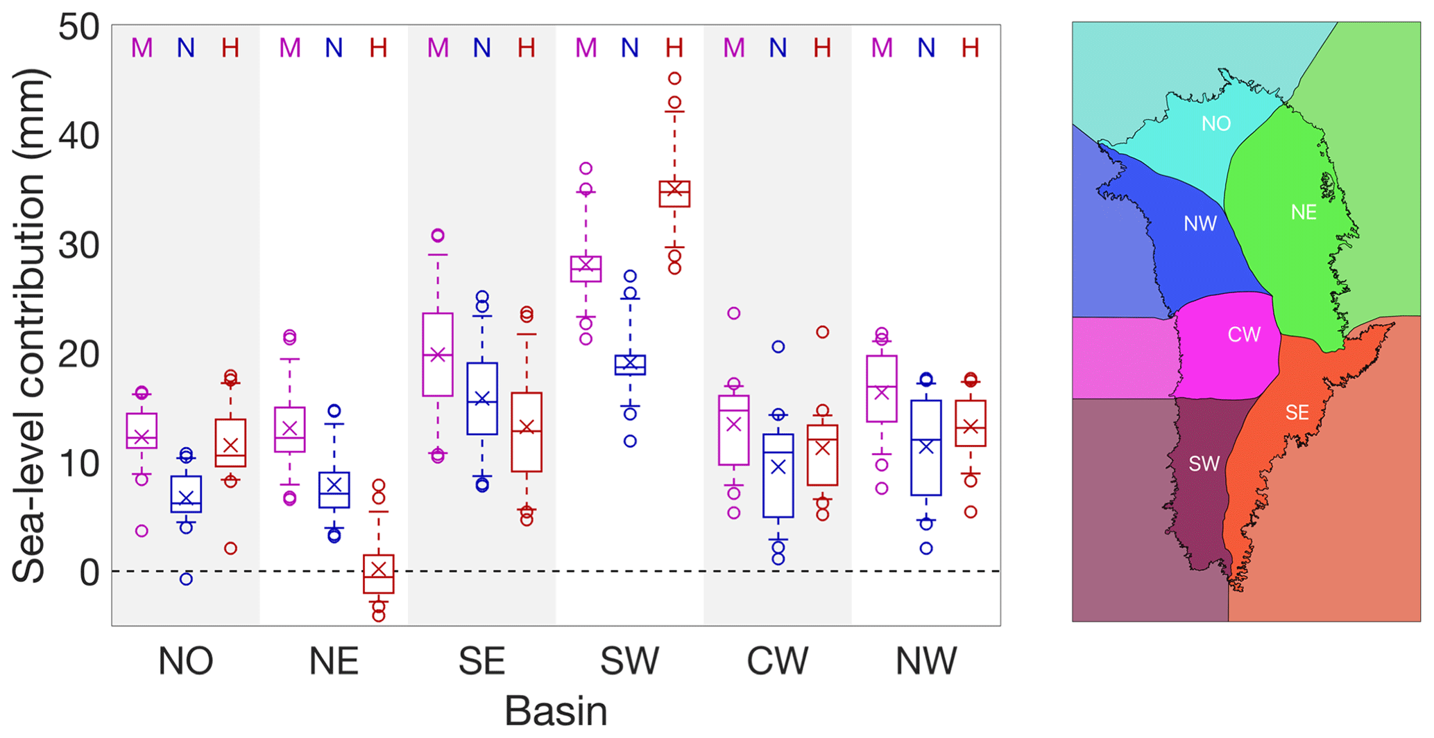
Figure 8Regional analysis of ice sheet changes for the three core GCMs (MIROC5–M, NorESM–N, HadGem2-ES–H) under scenario RCP8.5. The box plots show the ensemble median (line), mean (cross), interquartile range (box), range (whiskers) and outliers (circles). The basin definition is based on the IMBIE2-Rignot delineation (Rignot et al., 2011).
Ocean sensitivity
Uncertainty in the tidewater glacier retreat parameterization is sampled with three experiments under forcing scenario MIROC5-RCP8.5. Results for the three experiments are again compared per region (Fig. 9). The largest impact of differences in ocean forcing is visible in region CW, which is dominated by the response of Jakobshavn Isbrae, one of the largest outlet glaciers in Greenland. In the SW region, which is dominated by changes in SMB, differences in the ocean forcing have only a minor impact on the results, in line with findings described above. The mean spread due to ocean forcing over all ISMs that have performed the experiments (n=18) is 19 mm when summed over all six regions to get the Greenland-wide contributions.
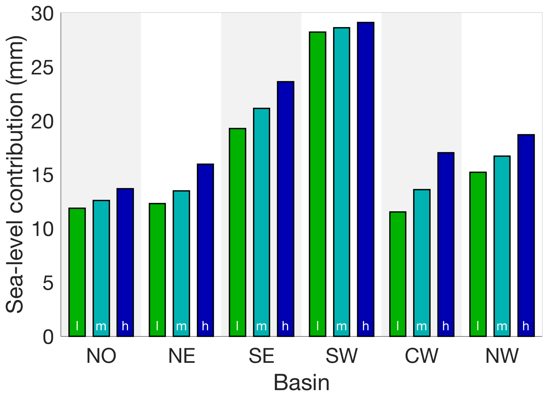
Figure 9Regional analysis of uncertainty due to ocean forcing. Ensemble mean sea-level contribution for MIROC5-RCP8.5 for low (green), medium (cyan) and high (blue) ocean forcing. The mean of the total Greenland contribution is 97, 101 and 116 mm for low, medium and high ocean forcing, respectively.
Combining projected sea-level contributions of the GrIS from all experiments, the ensemble mean and 2σ range for CMIP5 RCP8.5 is 90±50 mm (n=144), including six GCMs and three ocean sensitivities. The ensemble mean for RCP2.6 is 32±17 mm (n=21), sampling only one GCM (MIROC5) and one ocean sensitivity (medium). The corresponding ratios σ∕μ are 28 % for RCP8.5 and 27 % for RCP2.6, respectively, indicating that the relative uncertainty depends weakly on the ensemble mean and ensemble size. The ISM ensemble mean in experiment MIROC5-RCP8.5-medium is 101±40 mm (n=21), with %, meaning that the relative uncertainty reduces by only one-third when selecting one out of six GCMs. For each of the three RCP8.5 core experiments with medium ocean sensitivity, the absolute 2σ range, indicative of the ISM uncertainty, is ∼ 40 mm (n=21). For the extended experiments that have not been performed with some of the high and low extreme models, the absolute 2σ range is reduced at ∼ 30 mm (n=15). The 2σ range of the ISM means across the six GCMs, indicative of the climate forcing uncertainty, is of similar magnitude (36 mm) compared to the ISM uncertainty, while the spread of the means for three different ocean sensitivities is about half (19 mm), indicating the approximate relative importance of the three sources of uncertainty. Note that the reported GCM uncertainty based on only six models does not represent the full CMIP ensemble range.
4.4 Ice dynamic contribution
In this section we give an impression of the role of atmospheric and oceanic forcing and the contribution of ice dynamics. Separating the different forcing mechanisms completely requires dedicated single-forcing experiments that have been proposed as part of the extended experiments in the ISMIP6 protocol (Nowicki et al., 2020) but have not been studied here. Such analysis exceeds the scope of this paper and will be explored in a forthcoming publication.
To characterize the strength of the ocean forcing per region and forcing scenario, we have calculated the ice volume (in millimetres of sea-level equivalent) that would be instantaneously removed by the retreat parameterization from the observed ice sheet geometry (Fig. 10a). For an ice sheet model, the actual mass loss due to the retreat parameterization is considerably larger than the diagnostic shown here as the ice sheet responds dynamically to a retreat of the calving front. The ice flow accelerates and transports more mass to the marine margin that is subsequently removed by the masking, while the ice sheet is thinning further inland. This dynamic and non-linear response is the reason why physically based ice sheet models are indispensable to producing ice sheet projections for any timescale longer than a decade or 2. The diagnostic is contrasted by the integrated SMB anomaly over the observed geometry (Fig. 10b), which represents the dominant forcing for the resulting total sea-level contribution from the experiments (Fig. 10c). The SMB contribution is again calculated using the NOISM approach described above, taking into account elevation changes arising from the SMB anomaly itself to propagate the parameterized SMB-elevation feedback. In this case, however, we omit the tidewater glacier retreat in an atmosphere-only set-up.
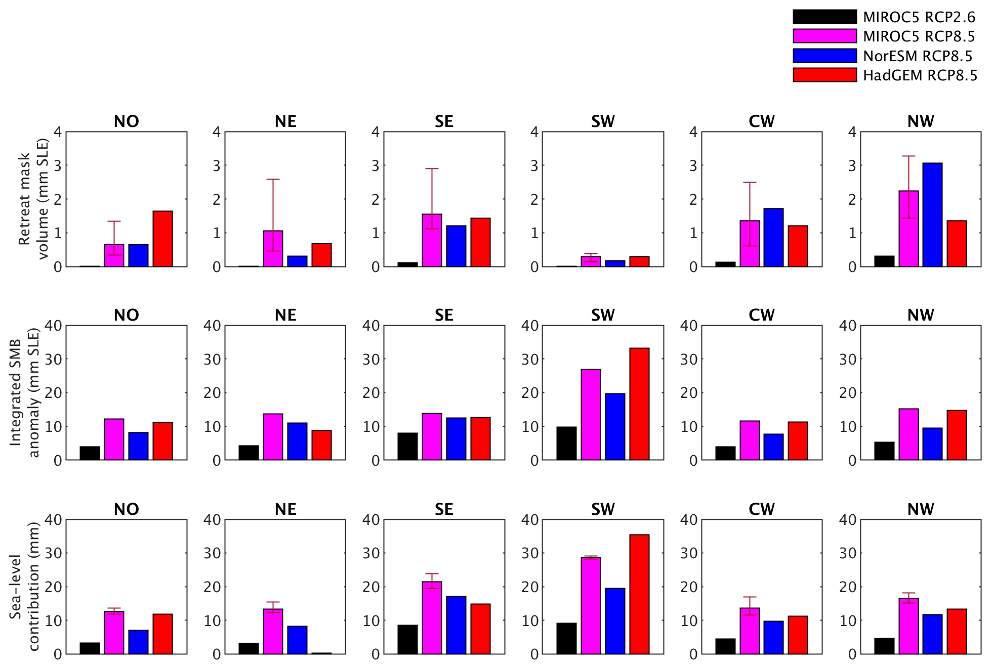
Figure 10Ocean and atmospheric forcing and sea-level response. (a) Volume instantaneously removed by the prescribed tidewater glacier retreat mask when applied to the observed geometry (Morlighem et al., 2017). (b) Integrated surface mass balance anomaly forcing over the observed geometry. (c) Ensemble mean sea-level contribution for all models using the standard forcing approach. Bars in (a) and (c) are for low and high ocean sensitivity. Note the different vertical scale for (a) compared to (b) and (c).
Visual inspection of the similarity between rows b and c suggests that the SMB anomaly is the governing forcing in our experiments, while oceanic forcing plays a more limited role for the results. In line with results described above, basin “SW” shows the lowest relative importance of oceanic forcing, and basin “NW” shows the largest.
Figure 11 illustrates the role of ice dynamic changes in our projections. We have calculated the mean dynamic contribution as the residual of the local mass change and the integrated SMB anomaly (Fig. 11a) as well as the corresponding standard deviation (Fig. 11b) for the ISM ensemble. Note that this diagnostic includes all ice thickness changes that are not explicitly related to SMB changes. The dynamic contribution (Fig. 11a) shows large negative values in places where the retreat parameterization has removed ice at the margins and from connected inland regions that have been thinning in response (which is therefore not explained by SMB changes). A region of positive dynamic contribution is visible in the land-terminated ablation zones around Greenland, where the negative SMB anomaly steepens the margins, which is compensated by dynamic thickening (Huybrechts and deWolde, 1999). Further inland, the corresponding upstream thinning is visible as a negative dynamic signal. The largest differences between models are located in regions of tidewater glacier retreat, where the amount of ice available for calving varies between models due to inaccuracies in the initial state.

Figure 11Dynamic contribution for experiment MIROC5-RCP8.5. (a) Ensemble mean dynamic ice thickness change residual and (b) standard deviation. See Fig. S9 in the Supplement for patterns for each individual model.
In the previous sections we have presented sea-level change projections for the GrIS over the 21st century and associated uncertainties due to forcing and ISM differences. Figure 12 summarizes the sea-level contribution from all experiments. The results indicate that the GrIS will continue to lose mass in both scenarios until 2100, with contributions of 90±50 and 32±17 mm to sea-level rise for RCP8.5 and RCP2.6, respectively.
Our estimates are around 10 mm lower compared to GrIS sea-level contributions reported by Fürst et al. (2015) for only one ice sheet model (101.5±32.5 and 42.3±18.0 mm for RCP8.5 and RCP2.6, respectively) but a larger range of CMIP5 GCMs (including the ones used in this study). However, their results include a present-day background trend of 0.32 mm yr−1 and span a period 15 years longer (2000–2100 vs. 2015–2100 in our study). Correcting for the length (assuming a linear trend of 0.32 mm yr−1 for the first 15 years) and assuming a minimum dynamic committed sea-level contribution of ∼ 6 mm (Price et al., 2011) to make the results more comparable leads to similar projections in the present study. Although our RCM-based forcing is a clear improvement over the positive degree-day approach used in Fürst et al. (2015), it has only a minor impact on the overall projections. The ocean forcing in their work was also driven by GCM-based ocean warming, but interaction with the ice was parameterized by prescribing tidewater glacier speed-up rather than by prescribing their retreat. Our estimates for RCP2.6 are also similar to results obtained with an ice sheet model forced by three CMIP5 GCMs (Rückamp et al., 2018). The AR5 projection for the GrIS under RCP8.5 in the year 2100 with respect to the 1986–2005 time mean is 150 mm (likely range of 90–280 mm). If similar corrections for the committed contribution and for the length as described above are applied to our results using observed (0.4–0.8 mm yr−1; The IMBIE Team, 2019) instead of modelled trends, our estimates overlap with the lower range of this assessment.
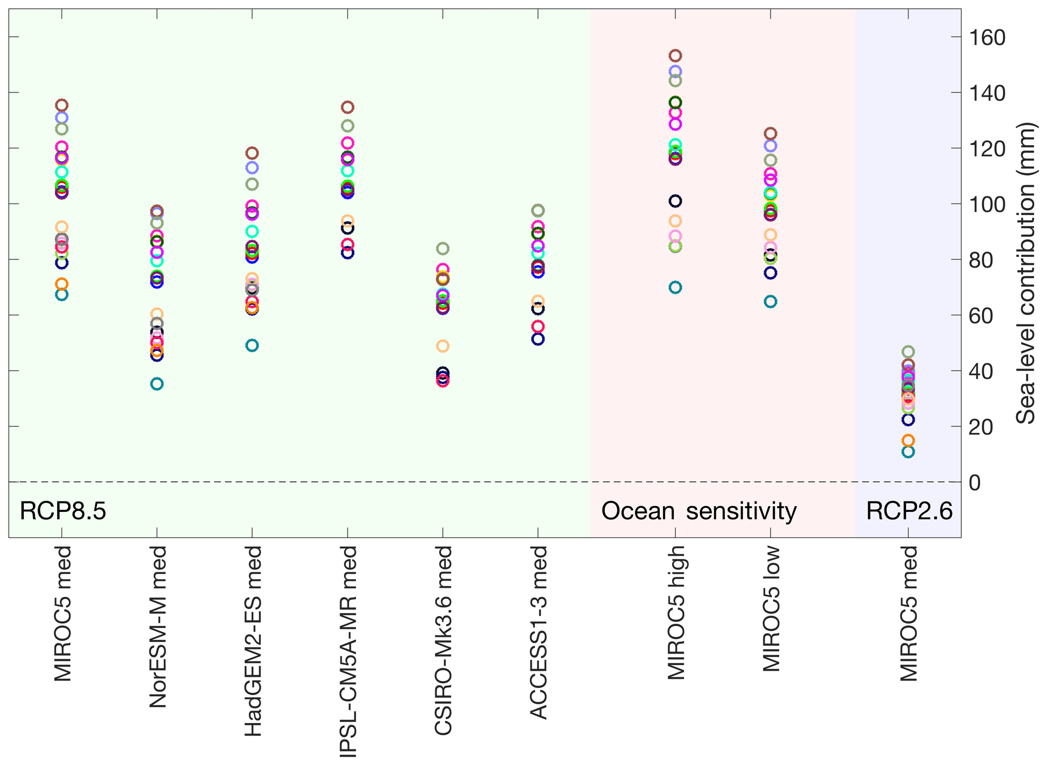
Figure 12Overview of sea-level projections for different CMIP5 experiments. All contributions are calculated relative to experiment “ctrl_proj”. The colour scheme is the same as in previous figures.
In cooperation with the GlacierMIP team (http://www.climate-cryosphere.org/mips/glaciermip, last access: 15 August 2020), we have attempted to mask out loosely connected glaciers and ice caps based on the RGI to avoid double-counting when our projections are used in global sea-level change assessments. However, next to a large resolution difference between ice sheet and glacier models, the fundamental differences of grid-based approaches in ice sheet modelling and “entity-based” approaches in glacier modelling are difficult to reconcile. Further work and a close interaction between our two communities are needed to improve solutions for these concerns.
While we consider the RCM-based SMB forcing to be a robust element in our projections, the computational requirements to produce such a forcing are immense and were only possible through the committed dedication of the MAR group. The large computational cost has also defined clear constraints on the number of GCMs and scenarios we could consider in our experiments and has ruled out a comparative analysis of RCM uncertainty. While different RCMs largely agree for simulations over the recent historical period (e.g. Fettweis et al., 2020), larger differences have to be expected for future projections where feedback mechanisms play a more important role. While we have not provided RCM uncertainty estimates in our projections, the SMB-dominated future response of the GrIS we find in our results suggests that those uncertainties would propagate almost directly into the projections.
The anomaly forcing approach chosen for SMB largely removes GCM and RCM biases and simplifies the experimental set-up and model comparison because all models apply the same forcing data. Nevertheless, it may be desirable to explore operating with the full SMB fields if consistency is a priority. Also, the anomaly approach is not suitable long-term because the assumption that unforced drift and forced signal combine linearly breaks down when both signals have become large. In any case it may be useful to operate with statistically bias-corrected GCM output that is in standard use by other comparison exercises (ISMIP; Warszawski et al., 2014) and avoid ad hoc corrections of GCM output.
Compared to the sophistication of fully physically based RCM SMB calculations, the implementation of the ocean forcing remains a crude approach that attempts to capture the complex interactions between the ocean and marine-terminating tidewater glaciers in Greenland in a very simplified way. Compared to earlier ad hoc approaches (e.g. Goelzer et al., 2013; Fürst et al., 2015; Calov et al., 2015; Beckmann et al., 2019), the advantage of the technique used (Slater et al., 2019, 2020) is its empirically based and transparent implementation. Nevertheless, large uncertainties are attached to this part of the projections and leave room for considerable improvements in the future. This requires a better physical understanding of the calving process (Benn et al., 2017) and high grid resolutions to resolve individual marine-terminating outlet glaciers. Existing calving laws need to be improved and included in ice flow models (e.g. Bondzio et al., 2016; Morlighem et al., 2016), which starts to be computationally feasible at a continental scale (e.g. Morlighem et al., 2019), as shown by the model submissions to the open framework in this study. Better understanding is also needed of the oceanographic processes that transport heat from the open ocean to the shelf, up fjords to calving fronts, and of the rate at which the ocean melts glacier calving fronts. We have generously sampled the uncertainty attached to the parameterization itself, but we cannot rule out additional factors that could bias ice sheet response from the far-field ocean temperature change and the local fjord circulation to the glacier front and its interaction with the local glacier bed geometry. Future work to improve understanding and representation of both the ocean forcing and ice dynamics is required.
Disentangling the importance of SMB and ocean forcing and the role of ice dynamics for sea-level change projections is an important scientific question that has strong bearing on our process understanding of the GrIS and its response to future climate change. With the experimental set-up for the present study, we were not able to address this issue sufficiently. Dedicated single-forcing experiments that have been proposed by ISMIP6 as part of the extended experiments will be analysed in a forthcoming publication to that end.
Our experimental set-up did not specifically encourage participants to achieve a good match of modelled historical mass changes with observations. To some extent this is related to the lack of knowledge about the past forcing and to the relative short history of high-quality observations compared to the dynamic response time of the GrIS. As a result, we are not in the position to quantify the present-day mass loss or the committed sea-level contribution from our experiments and have instead reported sea-level contributions relative to an unforced control experiment. This is an issue that needs to be addressed in future intercomparison exercises.
The largest difference between individual models in our ensemble and hence the ISM-related uncertainty in the projections arises from differences in the initial state. Inaccuracies in the initial state directly translate into differences in the applied SMB (masking), the amount of ice available for calving (thickness distribution), and, more generally, into the dynamic state of the ice sheet and its response to forcing. Improving initialization techniques further therefore remains a key priority for our community. The availability of high-quality observational datasets used as boundary conditions and to calibrate, validate and force ice sheet models has been a key ingredient in this endeavour and remains a fundamental requirement to reduce uncertainties in future ice sheet and sea-level change projections.
We present in the following a short description of the participating models and their initialization approach. Main model characteristics are summarized in Table A1. Further details may be found in the referenced model description papers and earlier publications of the individual groups.
Table A1Model characteristics. The numerical method is as follows. FD: finite difference; FE: finite element; FV: finite volume with adaptive mesh refinement. The ice flow is as follows. SIA: shallow-ice approximation; SSA: shallow-shelf approximation; HO: higher order; HYB: SIA and SSA combined. The initialization method is as follows. DAv: data assimilation of velocity; DAs: data assimilation of surface elevation; DAi: data assimilation of ice thickness; SP: spin-up; CYC: transient glacial cycle(s); NDm: nudging to ice mask; NDs: nudging to surface elevation. The initial SMB is as follows. RA1: RACMO2.1; RA3: RACMO2.3; HIR: HIRHAM5; MAR: MAR; BOX: BOX reconstruction (synthesis of simulation and data); ISMB: implied SMB. Velocity is as follows. RM: Rignot and Mouginot; J: Joughin et al. Bed and surface are as follows. M: Morlighem et al.; B: Bamber et al. Geothermal heat flux (GHF) is as follows. SR: Shapiro and Ritzwoller; G: Greve; MIX: see individual model description. Model resolution (Res) in kilometres. In case of heterogeneous grid resolution, the minimum and maximum resolutions are given.
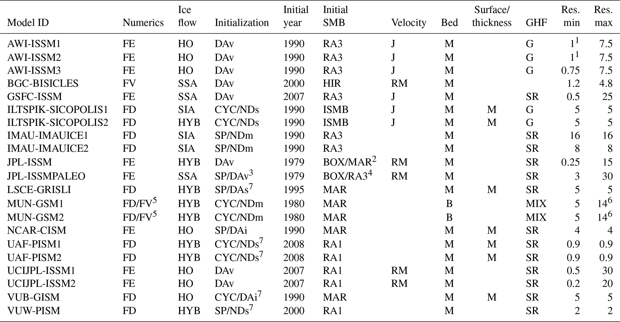
1 At the same minimum resolution, AWI-ISSM1 has considerably more small elements compared to AWI-ISSM2. 2 Climatology and historical spin-up from BOX but historical experiment from MAR anomalies. 3 SP with a base friction map of DAv (before palaeo run) that is scaled over time. 4 Climatology and historical spin-up from BOX but historical experiment from RACMO anomalies. 5 FD for ice dynamics, FV for ice thermodynamics. 6 0.25∘ longitude by 0.125∘ latitude. 7 CYC/SP used only for the ice temperature.
A1 AWI-ISSM
The Ice Sheet System Model (ISSM; Larour et al., 2012) is applied to the GrIS with Blatter–Pattyn higher-order approximation (Blatter, 1995; Pattyn, 2003). The initial state is defined by data assimilation of present-day conditions. Observed surface velocities (Joughin et al., 2010, 2016) are used to infer the basal friction coefficient at the ice base. The geometric input is BedMachine v3 (Morlighem et al., 2017) but excluding glaciers and ice caps surrounding the ice sheet proper. The initialization uses a 3-D temperature field that was generated by a combination of data assimilation and palaeoclimatic thermal spin-up (Rückamp et al., 2018). During all transient runs, we neglect an evolution of the thermal field. Grounding-line evolution is treated with a sub-grid parameterization scheme, which tracks the grounding-line position within the element (Seroussi et al., 2014). Basal melt rate below floating tongues is parameterized with a Beckmann–Goosse relationship (Beckmann and Goosse, 2003). The historical run employs SMB from RACMO2.3p2 (Noël et al., 2018) and no oceanic forcing. Model calculations are performed on a horizontally unstructured grid. The only difference between AWI-ISSM1, AWI-ISSM2 and AWI-ISSM3 is the spatial resolution. The minimum horizontal resolution at fast-flowing outlet glaciers is 1, 1 and 0.75 km for AWI-ISSM1, AWI-ISSM2 and AWI-ISSM3, respectively. AWI-ISSM1 uses static adaptive mesh refinement (Larour et al., 2012), while in AWI-ISSM2 and AWI-ISSM3 the minimum resolution is prescribed in fast-flowing regions (observed ice velocity > 200 m yr−1). Independent of the spatial resolution, the vertical discretization comprises 15 terrain-following layers refined towards the base. A detailed description of the model characteristics can be found in Rückamp et al. (2020).
A2 BGC-BISICLES
The method of initialization remains the same as in intMIP-Greenland (Goelzer et al., 2018) except that the ice surface is evolved with fjord bathymetry and bedrock elevation located outside the ice sheet interpolated from BedMachine v3 (Morlighem et al., 2017). All experiments use the ISMIP6 open approach, where the calving front is free to move. Its position is determined by advecting the area fraction of ice in the grid cells with the relative velocity of the front, which is the ice velocity at the calving front minus the calving rate in the normal direction to the front. The calving rate is a function of the melt rate given by Xu at al. (2013) and Rignot et al. (2016) relative to its mean value between 1997 and 2006. This approach models both melting along the front and solid ice calving. The historical run uses atmosphere and ocean forcing averaged over nine GCMs: ACCESS1.3-rcp85, CNRM-CM6-ssp126, CNRM-CM6-ssp585, CSIRO-Mk3.6-rcp85, HadGEM2-ES-rcp85, IPSL-CM5-MR-rcp85, MIROC5-rcp26, MIROC5-rcp85 and NorESM1-rcp85. For ctrl_proj, the calving rate at the front is equal to the normal ice velocity, i.e. the calving front is approximately stationary.
A3 GSFC-ISSM
The Ice Sheet System Model (ISSM; Larour et al., 2012) is initialized to present-day conditions by using BedMachine v3 geometry (Morlighem et al., 2017) and observed surface velocities (Joughin et al., 2016, 2017) to invert for the basal friction coefficient. The resolution of the mesh varies from 500 m in the fast flowing outlet glaciers and in regions where projected retreat occurs to 25 km in the slow-flowing interior. The ice viscosity is estimated from 1960 to 1989 surface temperatures from RACMO2.3p2 (Noël et al., 2018) and held constant during all simulations. To reduce spurious thickening signals, a 50-year relaxation is performed using a 1960–1989 mean SMB from RACMO2.3p2 (Noël et al., 2018). We estimate basal melt under floating ice by finding the difference between the model and 2003–2009 observed dynamic thickness change (Csatho et al., 2014) at the end of the relaxation. The difference is treated as the basal melt rate (floating ice only) and is held constant for the duration of the projections. The grounding line is allowed to evolve using a sub-element migration scheme (Seroussi et al., 2014). The calving front position is fixed and dictated by the ISMIP6 projected retreat masks.
A4 ILTSPIK-SICOPOLIS
The model SICOPOLIS version 5.1 (Greve and SICOPOLIS Developer Team, 2019; http://www.sicopolis.net/, last access: 15 August 2020) is applied to the GrIS with either shallow-ice dynamics (SICOPOLIS1) or hybrid shallow-ice–shelfy-stream dynamics (Bernales et al., 2017; SICOPOLIS2) for grounded ice. Floating ice is ignored. Ice thermodynamics are treated with the melting-CTS enthalpy method (ENTM) by Greve and Blatter (2016). The ice surface is assumed to be traction-free. Basal sliding under grounded ice is described by a Weertman–Budd-type sliding law with sub-melt sliding and subglacial hydrology (Kleiner and Humbert, 2014; Calov et al., 2018). The model is initialized by a palaeoclimatic spin-up over 134 000 years until 1990 that follows Greve (2019) closely. During the last 9000 years, the computed topography is continuously nudged towards the (slightly smoothed) observed present-day topography. Prior to 1000 years ago, this is done by the method described by Rückamp et al. (2019). For the last 1000 years, the “implied SMB” by Calov et al. (2018) with a relaxation time of 100 years is used instead. The latter limits the simulated ice sheet to its present-day extent. The basal sliding coefficient is determined individually for 20 different regions – the 19 basins by Zwally et al. (2012) plus a separate region for the Northeast Greenland Ice Stream (NEGIS; defined by ≥ 50 m yr−1 surface velocity) – by minimizing the root mean square deviation between simulated and observed logarithmic surface velocities. The historical run from 1990 until 2015 employs the MIROC5-RCP8.5 atmospheric forcing and no oceanic forcing. For the last 9000 years of the spin-up, the historical run and the future climate simulations, a regular (structured) grid with 5 km resolution is used. In the vertical, we use terrain-following coordinates with 81 layers in the ice domain and 41 layers in the thermal lithosphere layer below. The present-day surface temperature is parameterized (Fausto et al., 2009; Rückamp et al., 2019). The bed topography is BedMachine v3 (Morlighem et al., 2017), the geothermal heat flux is by Greve (2019), and glacial isostatic adjustment (GIA) is modelled by the local-lithosphere–relaxing-asthenosphere (LLRA) approach with a time lag of 3000 years (Le Meur and Huybrechts, 1996). A more detailed description of the set-up is given elsewhere (Greve et al., 2020).
A5 IMAU-IMAUICE
The model (de Boer et al., 2014) is initialized to a thermodynamically coupled steady state with constant, present-day boundary conditions for 61 kyr using the average 1960–1990 surface temperature and SMB from RACMO2.3 (van Angelen et al., 2014). Bedrock data are from Morlighem et al. (2017) and geothermal heat flux from Shapiro and Ritzwoller (2004). The model is run in SIA mode with ice sheet margins evolving freely within the observed ice mask, outside of which a negative SMB is applied. For IMAUICE1 (16 km resolution) we continue with fixed temperature for 11 kyr to get a dynamic steady state that we assign to the year 1959. The historical run (1960–2014) is forced with SMB anomalies from a downscaled RACMO product (Noël et al., 2016) and a historical extension of the retreat mask forcing. For IMAUICE2 the dynamic steady state from IMAUICE1 is interpolated to 8 km resolution and relaxed for 10 kyr before proceeding with the historical run.
A6 JPL-ISSM
The JPL-ISSM ice sheet model (Larour et al., 2012) configuration relies on the data assimilation of present-day conditions followed by a model relaxation and a historical spin-up, similar to Schlegel et al. (2016). For the calculation of stress balance, L1L2 (Hindmarsh, 2004; Schoof and Hindmarsh, 2010) is used over the entire domain with a resolution varying between 250 m in the areas of strongest gradients in surface velocity and along the margins to a resolution of 15 km in the interior. Bedrock topography is interpolated from BedMachine (Morlighem et al., 2017), and initial ice surface is from the GIMP dataset (Howat et al., 2014). Basal heat flux is from Shapiro and Ritzwoller (2004) and air temperature from RACMO2 (van Angelen et al., 2014). We use observed surface velocities (Rignot and Mouginot, 2012) to infer unknown basal friction at the base of the ice sheet (Morlighem et al., 2010). We then calculate ice temperature, assuming that the ice sheet is in a steady-state thermal equilibrium (Seroussi et al., 2013). This is followed by a relaxation of 4.2 kyr to reduce the initial unphysical transient behaviour resulting from errors and biases in the datasets and forcing (Schlegel et al., 2016) using a climatological mean surface mass balance from 1979 to 1988 (Box, 2013). Finally, we run a historical spin-up from 1840 through 1979 using the Box (2013) reconstruction of surface mass balance. Grounding-line migration is based on hydrostatic equilibrium and a sub-element scheme (Seroussi et al., 2014; Seroussi and Morlighem, 2018, SEM2 parameterization), and basal melting rates from the literature (Rignot, 2001; Rignot and Steffen, 2008; Seroussi et al., 2011; Prescott et al., 2003) are set under floating ice. The ice front is held static during all initialization, historic and control experiments, and there is a free-flux boundary condition at all ice margins. For the historical experiment, MAR 3.9 yearly anomalies in SMB (Fettweis et al., 2017) from the 1979–1988 mean are added to the spin-up SMB (i.e. the Box, 2013, 1979–1988 climatology). For the control experiment, the model is forced only with the spin-up SMB. During projection runs, the ISMIP6 SMB anomalies are imposed using an SMB gradient scheme (Helsen et al., 2012) on top of the spin-up SMB, and ISMIP6 retreat masks are imposed yearly, on 1 January of each year.
A7 JPL-ISSMPALEO
Initialization procedures are after Cuzzone et al. (2019). Bedrock topography is interpolated from the BedMachine dataset (Morlighem et al., 2014), which combines a mass conservation algorithm for the fast-flowing ice streams and kriging in the interior of the ice sheet. Initial ice thickness is from the GIMP dataset (Howat et al., 2014). Geothermal flux is from Shapiro and Riztwoller (2004), and air temperature is from Box (2013). We assimilate surface horizontal velocities derived from published 2008–2009 surface velocities (Rignot and Mouginot, 2012) to derive basal sliding on grounded ice and ice viscosity on floating ice. The model uses the higher-order ice flow approximation of Blatter (1995) and Pattyn (2003), which is extruded to five layers and uses higher-order vertical finite elements (Cuzzone et al., 2018) to compute the ice sheet thermal evolution. The initial friction coefficient is modified through time based upon variations in the simulated basal temperature following Cuzzone et al. (2019). The model is spun up over one glacial cycle (beginning 125 000 years ago) using a method whereby the 1840–1900 mean surface air temperature and precipitation (Box, 2013) are scaled back through time based upon isotopic variations in the Greenland Ice Core Project (GRIP) δO18 record (Danasgaard et al., 1993). We use the positive degree-day model of Tarasov and Peltier (1999) to derive the surface mass balance through time (degree-day factors; snow = 0.006 m ∘C−1 d−1, ice = 0.0083 m ∘C−1 d−1). From 1840 to 1979, the model is then forced with the surface mass balance history derived in Box (2013), and from 1979 to 2014, the RACMO2.3 (Noël et al., 2015) surface mass balance is used.
A8 LSCE-GRISLI
Here we used the GRISLI version 2.0 (Quiquet et al., 2018), which includes the analytical formulation of Schoof (2007) to compute the flux at the grounding line. Basal drag is computed with a power-law basal friction (Weertman, 1957). We use an iterative inversion method to infer a spatially variable basal drag coefficient that insures an ice thickness as close as possible to observations with a minimal model drift (Le clec'h et al., 2019). The model is run for 60 kyr with a fixed geometry (observed present-day) in order to equilibrate the temperature field. The basal drag is assumed to be constant for the forward experiments. The model uses finite differences on a staggered Arakawa C-grid in the horizontal plane at 5 km resolution with 21 vertical levels. Atmospheric forcing, namely near-surface air temperature and surface mass balance, is taken from the 1995–2014 climatological annual mean computed by the MAR version 3.9 regional atmospheric model. The initial ice sheet geometry, bedrock elevation and ice thickness are taken from the BedMachine v3 dataset (Morlighem et al., 2017), and the geothermal heat flux is from Shapiro and Ritzwoller (2004).
A9 MUN-GSM
The two models GSM1 and GSM2 are from a two-glacial-cycle run (starting at 240 ka) with 30 ensemble model parameters set to values from an ongoing calibration against various palaeo constraints (including relative sea level data and cosmogenic dates) along with topography fit to present day at the end of the transient run. The grid resolution is longitude–latitude, which translates to about 13.9 km in the latitudinal direction and goes down to about 5 km in the longitudinal direction near the northern edge of the ice sheet. For this intercomparison, the model was nudged to observed 2000 CE ice margins during the 1500 to 2000 CE interval. The model uses a 4 km deep permafrost-resolving bed thermal model with the deep geothermal heat flux set to a partially calibrated mix from Rogozhina et al. (2016), Fox Maule et al. (2009), Tarasov and Peltier (2003), and Pollack et al. (1993). The glacial cycles use a calibrated mix of climate forcings derived from the GRIP δ18O record (GICC05 chronology and Dansgaard et al., 1993, chronology), the synthetic temperature record from Barker et al. (2011) and PMIP III fields from GCM simulations (Braconnot et al., 2012). Surface mass balance depends on both positive degree days (PDDs) and (orbitally updated) monthly mean insolation. Ocean temperatures (for submarine ice melt) are derived from scaling the results of the TRACE deglacial simulation with CSSM3 (Liu et al., 2009). The two models differ in the soft-bedded basal drag used since 1500 CE. The GSM1 version uses a Coulomb-plastic soft-bed rheology, while the GSM2 version uses a linear Weertman-type basal drag law (as was used for the full glacial cycle run for both models). Both use a power law basal drag formulation for hard bed.
A10 NCAR-CISM
The Community Ice Sheet Model (CISM; Lipscomb et al., 2019) was run on a regular 4 km grid with 10 vertical layers using a depth-integrated higher-order velocity solver based on Goldberg (2011) and a basal-sliding law based on Schoof (2005). The ice sheet was initialized with present-day thickness and bed topography (Morlighem et al., 2017) and an idealized temperature profile. CISM was then spun up for 30 000 years with surface mass balance and surface temperature from a 1980–1999 climatology provided by the MAR regional climate model (Fettweis et al., 2017) and with basal heat fluxes from Shapiro and Ritzwoller (2004). During the spin-up, the model was nudged toward present-day thickness by adjusting friction coefficients in a basal-sliding power law. There is no dependence of basal sliding on basal temperature or water pressure. All floating ice was assumed to calve immediately. For partly grounded cells at the marine margin, basal shear stress was weighted using a grounding-line parameterization. By the end of the spin-up, the ice thickness, temperature and velocity fields were very close to steady-state. For the historical period (1990–2014), the model was run forward with SMB and surface temperature anomalies, including lapse-rate corrections, from the MAR simulation that provided the background climatology. Basal friction coefficients were held fixed at the values obtained during the spin-up.
A11 UAF-PISM
Ice sheet initial conditions are provided by the “calibrated” experiments in Aschwanden et al. (2016). The goal of an initialization procedure is to provide a present-day energy state which can currently not be obtained from observations alone. To define the energy state, a “standard” glacial cycle run was performed where the surface can evolve freely, similar to Aschwanden et al. (2013). The spin-up started at 125 kyr BP with the present-day topography from Howat et al. (2014) using a horizontal grid resolution of 9 km. The grid was refined to 6, 4.5 and 3 km at 25, 20 and 15 kyr BP, respectively. We used a positive degree-day scheme to compute the climatic mass balance from surface temperature (Fausto et al., 2009) and model-constrained precipitation (Ettema et al., 2009). The degree-day factors were the same as in Huybrechts and de Wolde (1999). Second, we accounted for palaeoclimatic variations by applying a scalar anomaly term derived from the GRIP ice core oxygen isotope record (Dansgaard et al., 1993) to the temperature field (Huybrechts, 2002). Then we adjusted mean annual precipitation in proportion to the mean annual air temperature change (Huybrechts, 2002). Finally, sea-level forcing, which determines the land area available for glaciation, is derived from the SPECMAP marine δ18O record (Imbrie et al., 1992). Using this as a starting point, we then ran a 100-year-long relaxation simulation at 900 m resolution to account for differences and updates in model physics, but we kept the ice surface close to observations using a flux correction (Aschwanden et al., 2016). The result is an initial state that is both close to the observed geometry (Howat et al., 2014) and surface speeds (Rignot and Mouginot, 2012) of 2008. For ISMIP6, the initial state was regridded to a horizontal resolution of 1 km as defined by ISMIP6.
A12 UCIJPL-ISSM
The ice sheet configuration is set up using data assimilation of present-day conditions (Morlighem et al., 2010). The bed topography is interpolated from the BedMachine Greenland v3 dataset (Morlighem et al., 2017). The initial ice surface topography is from the GIMPdem (Howat et al., 2014). For the thermal model, surface temperatures from Fausto et al. (2009) and geothermal heat flux from Shapiro and Ritzwoller (2004) are used. A higher-order model (HO) is used for the entire domain. The model for UCIJPL-ISSM1 has 14 vertical layers and a horizontal resolution varying between 0.5 km along the coast and 30 km inland, while UCIJPL-ISSM2 has 4 vertical layers with a horizontal resolution between 0.2 and 20 km. We perform the inversion of basal friction assuming that the ice is in a thermo-mechanical steady state. The ice temperature is updated as the basal friction changes, and the ice viscosity is changed accordingly. At the end of the inversion, basal friction, ice temperature and stresses are all consistent. After the data assimilation process, the model for UCIJPL-ISSM1 is relaxed for 50 years using the mean surface mass balance of 1961–1990 from RACMO (van Angelen et al., 2014) while keeping the temperature constant. The historical run was performed with SMB anomalies of MIROC5 provided by ISMIP6, with the fixed ice front for UCIJPL-ISSM1 and with the moving ice front for UCIJPL-ISSM2.
A13 VUB-GISM
VUB-GISM (Huybrechts, 2002; Fürst et al., 2015) is configured with the higher-order version, using a simplified resistance equation to describe the basal resistance (called SR HO in Fürst et al., 2013). GISM was initialized to the present-day geometry by assimilation of the observed ice thickness (Le clec'h et al., 2019). A steady state was assumed for the starting date of December 1989 using the 1960–1989 mean SMB from MAR forced by the MIROC5 climate. The iterative initialization method optimized both the basal sliding coefficient in unfrozen areas and the rate factor in Glen's flow law for frozen areas. The ice temperature and the initial velocity field needed in the initialization procedure were derived from a glacial spin-up with a freely evolving geometry over the last two glacial cycles with a synthesized temperature record based on ice-core data from Dome C, NGRIP, GRIP and GISP2 (Fürst et al., 2015). For this spin-up experiment, a PDD model was used with an observed precipitation field derived from the Bales et al. (2009) surface accumulation for the period 1950–2000 and scaled by 5 % ∘C−1. The ice temperature and velocity fields from the “free geometry present-day” were rescaled to the observed ice thickness (Morlighem et al., 2017) and excluded peripheral ice (Citterio et al., 2013). The historical experiment is run from January 1990 to December 2014 using the yearly SMB from MAR forced by MIROC5. For the projections, the standard retreat forcing and the parameterized SMB-height feedback from the ISMIP6 protocol are applied.
A14 VUW-PISM
We use an identical approach to the one described in Golledge et al. (2019). Starting from initial bedrock and ice thickness conditions from Morlighem et al. (2017) together with reference climatology from Ettema et al. (2009), we run a multi-stage spin-up that guarantees well-evolved thermal and dynamic conditions without loss of accuracy in terms of geometry. This is achieved through an iterative nudging procedure, in which incremental grid refinement steps are employed that also include resetting of ice thicknesses to initial values. Drift is thereby eliminated, but thermal evolution is preserved by remapping temperature fields at each stage. In summary, we start with an initial 20 km resolution 5-year smoothing run in which only the shallow-ice approximation is used. Then, holding the ice geometry fixed, we run a 125 000-year, 20 km resolution thermal-evolution simulation in which temperatures are allowed to equilibrate. Refining the grid to 10 km and resetting bed elevations and ice thicknesses, we run a further 3000 years using full model physics, then refine the grid to 5 km for a further 1000 years, then refine the grid to 2 km for 500 years. The resultant configuration is then used as the starting point for each of our forward experiments.
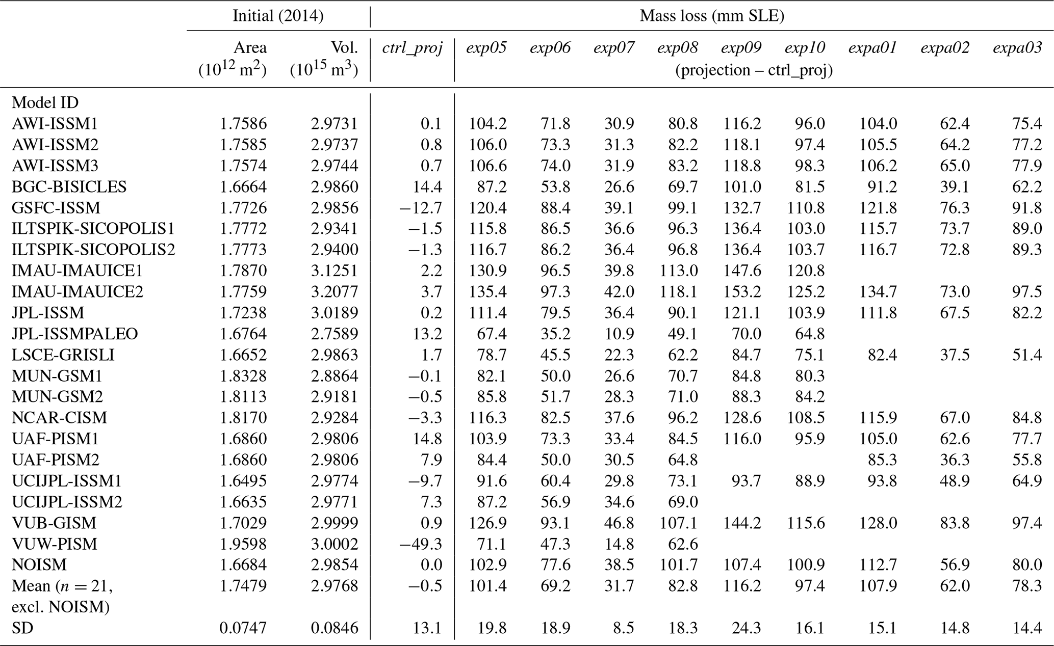
Table B1Modelled present-day ice sheet area, ice volume and mass change in future experiments for all participating models.
Data processing, analysis and plotting scripts are available on GitHub (https://github.com/ismip, last access: 15 August 2020) and are archived in permanent repositories on Zenodo with digital object identifiers https://doi.org/10.5281/zenodo.3939115 (Goelzer, 2020a) and https://doi.org/10.5281/zenodo.3939113 (Goelzer, 2020b).
The recomputed scalar variables analysed in this paper are available on Zenodo with digital object identifier https://doi.org/10.5281/zenodo.3939037 (Goelzer, 2020c). The forcing datasets are available through the ISMIP6 wiki (http://www.climate-cryosphere.org/wiki/index.php?title=ISMIP6_wiki_page, last access: 15 August 2020) and will also be archived in a publicly available repository (see assets tab of this paper). The 2-D fields of model output from the simulations described in this paper will be made available in the CMIP6 archive through the Earth System Grid Federation (ESGF; https://esgf.llnl.gov/, last access: 15 August 2020).
In order to document CMIP6's scientific impact and enable ongoing support of CMIP, users are obligated to acknowledge CMIP6, the participating modelling groups and the ESGF centres (see details on the CMIP panel website at http://www.wcrp-climate.org/index.php/wgcm-cmip/about-cmip, last access: 15 August 2020).
The supplement related to this article is available online at: https://doi.org/10.5194/tc-14-3071-2020-supplement.
HG, SN, AP, EL, HS, WHL, JG, AA-O and AS designed the project with help from CA, AB, DF, CL, MM, DS, RS and FS. Model results were contributed to the project by HG, SN, AP, HS, WHL, AA, RC, CC, YC, JC, CD, DF, NRG, RG, AH, PH, SL, VL, GL, DPL, MM, IN, AQ, MR, NS and LT. ES, CA, PA, DF, XF, MM and DS provided or prepared input and forcing data. ES and HG have processed the model output data. HG wrote the manuscript with comments from all co-authors.
Xavier Fettweis, Eric Larour and Michiel van den Broeke serve as topical editors for the journal. William H. Lipscomb, Sophie Nowicki, Helene Seroussi, Ayako Abe-Ouchi and Robin S. Smith are editors of the special issue “The Ice Sheet Model Intercomparison Project for CMIP6 (ISMIP6)”.
This article is part of the special issue “The Ice Sheet Model Intercomparison Project for CMIP6 (ISMIP6)”. It is not associated with a conference.
We thank the Climate and Cryosphere (CliC) project for providing support for ISMIP6 through sponsoring workshops, hosting the ISMIP6 website and wiki, and promoting ISMIP6. We acknowledge the World Climate Research Programme and its Working Group on Coupled Modelling for coordinating and promoting CMIP5 and CMIP6. We thank the climate modelling groups for producing and making available their model output; the Earth System Grid Federation (ESGF) for archiving the CMIP data and providing access; the University at Buffalo for ISMIP6 data distribution and upload; and the multiple funding agencies who support CMIP5, CMIP6 and the ESGF. We thank the ISMIP6 steering committee, the ISMIP6 model selection group and ISMIP6 dataset preparation group for their continuous engagement in defining ISMIP6. We thank the editor and the two reviewers for supporting the publication of this paper.
This is ISMIP6 contribution no. 10.
Heiko Goelzer has received funding from the programme of the Netherlands Earth System Science Centre (NESSC), financially supported by the Dutch Ministry of Education, Culture and Science (OCW), under grant no. 024.002.001. For NCAR-CISM this material is based upon work supported by the National Center for Atmospheric Research, which is a major facility sponsored by the National Science Foundation under cooperative agreement no. 1852977. Computing and data storage resources, including the Cheyenne supercomputer (https://doi.org/10.5065/D6RX99HX), were provided by the Computational and Information Systems Laboratory (CISL) at NCAR. Alice Barthel was supported by the US Department of Energy (DOE) Office of Science Regional and Global Model Analysis (RGMA) component of the Earth and Environmental System Modeling (EESM) programme (HiLAT-RASM project) and the DOE Office of Science (Biological and Environmental Research) Early Career Research programme. Philippe Huybrechts and Sébastien Le clec'h acknowledge support from the iceMOD project funded by the Research Foundation – Flanders (FWO-Vlaanderen). Ralf Greve and Chris Chambers were supported by the Japan Society for the Promotion of Science (JSPS) KAKENHI (grant no. JP16H02224). Ralf Greve was supported by JSPS KAKENHI (grant no. JP17H06104) and by the Arctic Challenge for Sustainability (ArCS) project of the Japanese Ministry of Education, Culture, Sports, Science and Technology (MEXT) under programme grant no. JPMXD1300000000. Reinhard Calov was funded by the Bundesministerium für Bildung und Forschung (BMBF; grants PalMod-1.1 and PalMod-1.3). Support for Nicholas Golledge and Daniel Lowry was provided by the New Zealand Ministry of Business Innovation and Employment (contract RTVU1705). Martin Rückamp received support from the Helmholtz Climate Initiative REKLIM (Regional Climate Change). The AWI-ISSM simulations were run on the DKRZ HPC system Mistral under grant ab1073. Jonathan Gregory and Robin S. Smith were supported by the National Centre for Atmospheric Science, funded by the UK National Environment Research Council. Work was performed by Nicole Schlegel and Helene Seroussi at the Jet Propulsion Laboratory, California Institute of Technology, under a contract with the National Aeronautics and Space Administration. Funding was provided by grants from the Jet Propulsion Laboratory Research Technology and Development programme. Sophie Nowicki, Erika Simon, Isabel Nias, Helene Seroussi and Nicole Schlegel were supported by the NASA programmes Cryosphere Sciences; Sea Level Change Team; and Modeling, Analysis, and Prediction. Mathieu Morlighem and Joshua Cuzzone were funded by the National Science Foundation's ARCSS programme (grant no. 1504230). Youngmin Choi was supported by the NASA Earth and Space Science Fellowship programme grant (grant no. 80NSSC17K0409). Denis Felikson was supported by an appointment to the NASA Postdoctoral Program at the NASA Goddard Space Flight Center, administered by Universities Space Research Association under contract with NASA. Fiammetta Straneo and Donald A. Slater received support from the NSF.
This paper was edited by Christina Hulbe and reviewed by Fuyuki SAITO and one anonymous referee.
Aschwanden, A., Aðalgeirsdóttir, G., and Khroulev, C.: Hindcasting to measure ice sheet model sensitivity to initial states, The Cryosphere, 7, 1083–1093, https://doi.org/10.5194/tc-7-1083-2013, 2013.
Aschwanden, A., Fahnestock, M. A., and Truffer, M.: Complex Greenland outlet glacier flow captured, Nat. Commun., 7, 10524, https://doi.org/10.1038/ncomms10524, 2016.
Bales, R. C., Guo, Q., Shen, D., Mcconnell, J. R., Du, G., Burkhart, J. F., Spikes, V. B., Hanna, E., and Cappelen, J.: Annual accumulation for Greenland updated using ice core data developed during 2000–2006 and analysis of daily coastal meteorological data, J. Geophys. Res., 114, D06116, https://doi.org/10.1029/2008JD011208, 2009.
Barker, S., Knorr, G., Edwards, R. L., Parrenin, F., Putnam, A. E., Skinner, L. C., Wolff, E., and Ziegler, M.: 800,000 Years of Abrupt Climate Variability, Science, 334, 347–351, https://doi.org/10.1126/science.1203580, 2011.
Barthel, A., Agosta, C., Little, C. M., Hattermann, T., Jourdain, N. C., Goelzer, H., Nowicki, S., Seroussi, H., Straneo, F., and Bracegirdle, T. J.: CMIP5 model selection for ISMIP6 ice sheet model forcing: Greenland and Antarctica, The Cryosphere, 14, 855–879, https://doi.org/10.5194/tc-14-855-2020, 2020.
Beckmann, A. and Goosse, H.: A parameterization of ice shelf-ocean interaction for climate models, Ocean Modell., 5, 157–170, https://doi.org/10.1016/S1463-5003(02)00019-7, 2003.
Beckmann, J., Perrette, M., Beyer, S., Calov, R., Willeit, M., and Ganopolski, A.: Modeling the response of Greenland outlet glaciers to global warming using a coupled flow line–plume model, The Cryosphere, 13, 2281–2301, https://doi.org/10.5194/tc-13-2281-2019, 2019.
Benn, D. I., Cowton, T., Todd, J., and Luckman, A.: Glacier Calving in Greenland, Curr. Clim. Change Rep., 3, 282–290, https://doi.org/10.1007/s40641-017-0070-1, 2017.
Bernales, J., Rogozhina, I., Greve, R., and Thomas, M.: Comparison of hybrid schemes for the combination of shallow approximations in numerical simulations of the Antarctic Ice Sheet, The Cryosphere, 11, 247–265, https://doi.org/10.5194/tc-11-247-2017, 2017.
Blatter, H.: Velocity and stress fields in grounded glaciers: a simple algorithm for including deviatoric stress gradients, J. Glaciol., 41, 333–344, https://doi.org/10.3189/S002214300001621X, 1995.
Bondzio, J. H., Seroussi, H., Morlighem, M., Kleiner, T., Rückamp, M., Humbert, A., and Larour, E. Y.: Modelling calving front dynamics using a level-set method: application to Jakobshavn Isbræ, West Greenland, The Cryosphere, 10, 497–510, https://doi.org/10.5194/tc-10-497-2016, 2016.
Box, J.: Greenland Ice Sheet Mass Balance Reconstruction. Part II: Surface Mass Balance (1840–2010), J. Clim., 26, 6974–6989, https://doi.org/10.1175/jcli-d-12-00518.1, 2013.
Braconnot, P., Harrison, S. P., Kageyama, M., Bartlein, P. J., Masson-Delmotte, V., Abe-Ouchi, A., Otto-Bliesner, B., and Zhao, Y.: Evaluation of climate models using palaeoclimatic data, Nat. Clim. Change, 2, 417–424, https://doi.org/10.1038/nclimate1456, 2012.
Calov, R., Beyer, S., Greve, R., Beckmann, J., Willeit, M., Kleiner, T., Rückamp, M., Humbert, A., and Ganopolski, A.: Simulation of the future sea level contribution of Greenland with a new glacial system model, The Cryosphere, 12, 3097–3121, https://doi.org/10.5194/tc-12-3097-2018, 2018.
Calov, R., Robinson, A., Perrette, M., and Ganopolski, A.: Simulating the Greenland ice sheet under present-day and palaeo constraints including a new discharge parameterization, The Cryosphere, 9, 179–196, https://doi.org/10.5194/tc-9-179-2015, 2015.
Church, J. A., Clark, P. U., Cazenave, A., Gregory, J. M., Jevrejeva, S., Levermann, A., Merrifield, M. A., Milne, G. A., Nerem, R. S., Nunn, P. D., Payne, A. J., Pfeffer, W. T., Stammer, D., and Unnikrishnan, A. S.: Sea Level Change, in: Climate Change 2013: The Physical Science Basis, Contribution of Working Group I to the Fifth Assessment Report of the Intergovernmental Panel on Climate Change, edited by: Stocker, T. F., Qin, D., Plattner, G.-K., Tignor, M., Allen, S. K., Boschung, J., Nauels, A., Xia, Y., Bex, V., and Midgley, P. M., Cambridge University Press, Cambridge, UK, New York, NY, USA, 1137–1216, 2013.
Citterio, M. and Ahlstrøm, A. P.: Brief communication “The aerophotogrammetric map of Greenland ice masses”, The Cryosphere, 7, 445–449, https://doi.org/10.5194/tc-7-445-2013, 201
Cogley, J. G.: Area of the Ocean, Mar. Geod., 35, 379–388, https://doi.org/10.1080/01490419.2012.709476, 2012.
Csatho, B. M., Schenk, A. F., van der Veen, C. J., Babonis, G., Duncan, K., Rezvanbehbahani, S., van den Broeke, M. R., Simonsen, S. B., Nagarajan, S., and van Angelen, J. H.: Laser altimetry reveals complex pattern of Greenland Ice Sheet dynamics, P. Natl. Acad. Sci. USA, 111, 18478–18483, https://doi.org/10.1073/pnas.1411680112, 2014.
Cuzzone, J. K., Morlighem, M., Larour, E., Schlegel, N., and Seroussi, H.: Implementation of higher-order vertical finite elements in ISSM v4.13 for improved ice sheet flow modeling over paleoclimate timescales, Geosci. Model Dev., 11, 1683–1694, https://doi.org/10.5194/gmd-11-1683-2018, 2018.
Cuzzone, J. K., Schlegel, N.-J., Morlighem, M., Larour, E., Briner, J. P., Seroussi, H., and Caron, L.: The impact of model resolution on the simulated Holocene retreat of the southwestern Greenland ice sheet using the Ice Sheet System Model (ISSM), The Cryosphere, 13, 879–893, https://doi.org/10.5194/tc-13-879-2019, 2019.
Dansgaard, W., Johnsen, S. J., Clausen, H. B., Dahl-Jensen, D., Gundestrup, N. S., Hammer, C. U., Hvidberg, C. S., Steffensen, J. P., Sveinbjoernsdottir, A. E., Jouzel, J., and Bond, G. C.: Evidence for general instability of past climate from a 250-kyr ice-core record, Nature, 364, 218–220, https://doi.org/10.1038/364218a0, 1993.
de Boer, B., Stocchi, P., and van de Wal, R. S. W.: A fully coupled 3-D ice-sheet–sea-level model: algorithm and applications, Geosci. Model Dev., 7, 2141–2156, https://doi.org/10.5194/gmd-7-2141-2014, 2014.
Edwards, T. L., Fettweis, X., Gagliardini, O., Gillet-Chaulet, F., Goelzer, H., Gregory, J. M., Hoffman, M., Huybrechts, P., Payne, A. J., Perego, M., Price, S., Quiquet, A., and Ritz, C.: Effect of uncertainty in surface mass balance–elevation feedback on projections of the future sea level contribution of the Greenland ice sheet, The Cryosphere, 8, 195–208, https://doi.org/10.5194/tc-8-195-2014, 2014.
Edwards, T. L., Fettweis, X., Gagliardini, O., Gillet-Chaulet, F., Goelzer, H., Gregory, J. M., Hoffman, M., Huybrechts, P., Payne, A. J., Perego, M., Price, S., Quiquet, A., and Ritz, C.: Probabilistic parameterisation of the surface mass balance–elevation feedback in regional climate model simulations of the Greenland ice sheet, The Cryosphere, 8, 181–194, https://doi.org/10.5194/tc-8-181-2014, 2014.
Ettema, J., Van Den Broeke, M. R., Van Meijgaard, E., Van De Berg, W. J., Bamber, J. L., Box, J. E., and Bales, R. C.: Higher surface mass balance of the Greenland ice sheet revealed by high-resolution climate modeling, Geophys. Res. Lett., 36, L12501, https://doi.org/10.1029/2009GL038110, 2009.
Eyring, V., Bony, S., Meehl, G. A., Senior, C. A., Stevens, B., Stouffer, R. J., and Taylor, K. E.: Overview of the Coupled Model Intercomparison Project Phase 6 (CMIP6) experimental design and organization, Geosci. Model Dev., 9, 1937–1958, https://doi.org/10.5194/gmd-9-1937-2016, 2016.
Fausto, R. S., Ahlstrom, A. P., Van As, D., Boggild, C. E., and Johnsen, S. J.: A new present-day temperature parameterization for Greenland, J. Glaciol., 55, 95–105, https://doi.org/10.3189/002214309788608985, 2009.
Fettweis, X., Box, J. E., Agosta, C., Amory, C., Kittel, C., Lang, C., van As, D., Machguth, H., and Gallée, H.: Reconstructions of the 1900–2015 Greenland ice sheet surface mass balance using the regional climate MAR model, The Cryosphere, 11, 1015–1033, https://doi.org/10.5194/tc-11-1015-2017, 2017.
Fettweis, X., Franco, B., Tedesco, M., van Angelen, J. H., Lenaerts, J. T. M., van den Broeke, M. R., and Gallée, H.: Estimating the Greenland ice sheet surface mass balance contribution to future sea level rise using the regional atmospheric climate model MAR, The Cryosphere, 7, 469–489, https://doi.org/10.5194/tc-7-469-2013, 2013.
Fettweis, X., Hofer, S., Krebs-Kanzow, U., Amory, C., Aoki, T., Berends, C. J., Born, A., Box, J. E., Delhasse, A., Fujita, K., Gierz, P., Goelzer, H., Hanna, E., Hashimoto, A., Huybrechts, P., Kapsch, M.-L., King, M. D., Kittel, C., Lang, C., Langen, P. L., Lenaerts, J. T. M., Liston, G. E., Lohmann, G., Mernild, S. H., Mikolajewicz, U., Modali, K., Mottram, R. H., Niwano, M., Noël, B., Ryan, J. C., Smith, A., Streffing, J., Tedesco, M., van de Berg, W. J., van den Broeke, M., van de Wal, R. S. W., van Kampenhout, L., Wilton, D., Wouters, B., Ziemen, F., and Zolles, T.: GrSMBMIP: Intercomparison of the modelled 1980–2012 surface mass balance over the Greenland Ice sheet, The Cryosphere Discuss., https://doi.org/10.5194/tc-2019-321, in review, 2020.
Fox Maule, C., Purucker, M. E., and Olsen, N.: Inferring magnetic crustal thickness and geothermal heat flux from crustal magnetic field models, Danish Climate Centre Report, 09–09, 2009.
Fürst, J. J., Goelzer, H., and Huybrechts, P.: Effect of higher-order stress gradients on the centennial mass evolution of the Greenland ice sheet, The Cryosphere, 7, 183–199, https://doi.org/10.5194/tc-7-183-2013, 2013.
Fürst, J. J., Goelzer, H., and Huybrechts, P.: Ice-dynamic projections of the Greenland ice sheet in response to atmospheric and oceanic warming, The Cryosphere, 9, 1039–1062, https://doi.org/10.5194/tc-9-1039-2015, 2015.
Goelzer, H.: ismip/ismip6-gris-results-processing: v1.0.0, Zenodo, https://doi.org/10.5281/zenodo.3939115, 2020a.
Goelzer, H.: ismip/ismip6-gris-analysis: v1.0.0, Zenodo, https://doi.org/10.5281/zenodo.3939113, 2020b.
Goelzer, H.: Dataset for “The future sea-level contribution of the Greenland ice sheet: a multi-model ensemble study of ISMIP6”, Zenodo, https://doi.org/10.5281/zenodo.3939037, 2020c.
Goelzer, H., Huybrechts, P., Fürst, J. J., Andersen, M. L., Edwards, T. L., Fettweis, X., Nick, F. M., Payne, A. J., and Shannon, S. R.: Sensitivity of Greenland ice sheet projections to model formulations, J. Glaciol., 59, 733–749, https://doi.org/10.3189/2013JoG12J182, 2013.
Goelzer, H., Robinson, A., Seroussi, H., and van de Wal, R. S. W.: Recent Progress in Greenland Ice Sheet Modelling, Curr. Clim. Change Rep., 3, 291-302, https://doi.org/10.1007/s40641-017-0073-y, 2017.
Goelzer, H., Nowicki, S., Edwards, T., Beckley, M., Abe-Ouchi, A., Aschwanden, A., Calov, R., Gagliardini, O., Gillet-Chaulet, F., Golledge, N. R., Gregory, J., Greve, R., Humbert, A., Huybrechts, P., Kennedy, J. H., Larour, E., Lipscomb, W. H., Le clec'h, S., Lee, V., Morlighem, M., Pattyn, F., Payne, A. J., Rodehacke, C., Rückamp, M., Saito, F., Schlegel, N., Seroussi, H., Shepherd, A., Sun, S., van de Wal, R., and Ziemen, F. A.: Design and results of the ice sheet model initialisation experiments initMIP-Greenland: an ISMIP6 intercomparison, Cryosphere, 12, 1433-1460, https://doi.org/10.5194/tc-12-1433-2018, 2018.
Goelzer, H., Noël, B. P. Y., Edwards, T. L., Fettweis, X., Gregory, J. M., Lipscomb, W. H., van de Wal, R. S. W., and van den Broeke, M. R.: Remapping of Greenland ice sheet surface mass balance anomalies for large ensemble sea-level change projections, The Cryosphere, 14, 1747–1762, https://doi.org/10.5194/tc-14-1747-2020, 2020a.
Goelzer, H., Coulon, V., Pattyn, F., de Boer, B., and van de Wal, R.: Brief communication: On calculating the sea-level contribution in marine ice-sheet models , The Cryosphere, 14, 833–840, https://doi.org/10.5194/tc-14-833-2020, 2020b.
Goldberg, D. N.: A variationally derived, depth-integrated approximation to a higher-order glaciological flow model, J. Glaciol., 57, 157–170, https://doi.org/10.3189/002214311795306763, 2011.
Golledge, N. R., Keller, E. D., Gomez, N., Naughten, K. A., Bernales, J., Trusel, L. D., and Edwards, T. L.: Global environmental consequences of twenty-first-century ice-sheet melt, Nature, 566, 65–72, https://doi.org/10.1038/s41586-019-0889-9, 2019.
Gregory, J. M., Griffies, S. M., Hughes, C. W., Lowe, J. A., Church, J. A., Fukimori, I., Gomez, N., Kopp, R. E., Landerer, F., Cozannet, G. L., Ponte, R. M., Stammer, D., Tamisiea, M. E., and van de Wal, R. S. W.: Concepts and Terminology for Sea Level: Mean, Variability and Change, Both Local and Global, Surv. Geophys., 40, 1251–1289, https://doi.org/10.1007/s10712-019-09525-z, 2019.
Greve, R.: Geothermal heat flux distribution for the Greenland ice sheet, derived by combining a global representation and information from deep ice cores, Polar Data Journal, 3, 22-36, https://doi.org/10.20575/00000006, 2019.
Greve, R. and Blatter, H.: Comparison of thermodynamics solvers in the polythermal ice sheet model SICOPOLIS, Polar Sci., 10, 11–23, https://doi.org/10.1016/j.polar.2015.12.004, 2016.
Greve, R. and SICOPOLIS Developer Team: SICOPOLIS v5.1, Zenodo, https://doi.org/10.5281/zenodo.3727511, 2019.
Greve, R., Chambers, C., and Calov, R.: ISMIP6 future projections for the Greenland ice sheet with the model SICOPOLIS, Technical report, Zenodo, https://doi.org/10.5281/zenodo.3971251, 2020.
Helsen, M. M., van de Wal, R. S. W., van den Broeke, M. R., van de Berg, W. J., and Oerlemans, J.: Coupling of climate models and ice sheet models by surface mass balance gradients: application to the Greenland Ice Sheet, The Cryosphere, 6, 255–272, https://doi.org/10.5194/tc-6-255-2012, 2012.
Hindmarsh, R. C. A.: A numerical comparison of approximations to the Stokes equations used in ice sheet and glacier modeling, J. Geophys. Res.-Earth Surf., 109, F01012, https://doi.org/10.1029/2003JF000065, 2004.
Howat, I. M., Negrete, A., and Smith, B. E.: The Greenland Ice Mapping Project (GIMP) land classification and surface elevation data sets, The Cryosphere, 8, 1509–1518, https://doi.org/10.5194/tc-8-1509-2014, 2014.
Huybrechts, P.: Sea-level changes at the LGM from ice-dynamic reconstructions of the Greenland and Antarctic ice sheets during the glacial cycles, Quat. Sci. Rev., 21, 203–231, https://doi.org/10.1016/S0277-3791(01)00082-8, 2002.
Huybrechts, P. and de Wolde, J.: The dynamic response of the Greenland and Antarctic ice sheets to multiple-century climatic warming, J. Clim., 12, 2169–2188, https://doi.org/10.1175/1520-0442(1999)012<2169:TDROTG>2.0.CO;2, 1999.
Huybrechts, P., Janssens, I., Poncin, C., and Fichefet, T.: The response of the Greenland ice sheet to climate changes in the 21st century by interactive coupling of an AOGCM with a thermomechanical ice-sheet model, Ann. Glaciol., 35, 409–415, https://doi.org/10.3189/172756402781816537, 2002.
Imbrie, J., Boyle, E. A., Clemens, S. C., Duffy, A., Howard, W. R., Kukla, G., Kutzbach, J., Martinson, D. G., McIntyre, A., Mix, A. C., Molfino, B., Morley, J. J., Peterson, L. C., Pisias, N. G., Prell, W. L., Raymo, M. E., Shackleton, N. J., and Toggweiler, J. R.: On the Structure and Origin of Major Glaciation Cycles 1. Linear Responses to Milankovitch Forcing, Paleoceanography, 7, 701–738, https://doi.org/10.1029/92PA02253, 1992.
Joughin, I., Smith, B., Howat, I., and Scambos, T.: MEaSUREs Multi-year Greenland Ice Sheet Velocity Mosaic, Version 1, Boulder, Colorado USA, NASA National Snow and Ice Data Center Distributed Active Archive Center, https://doi.org/10.5067/QUA5Q9SVMSJG, 2016.
Joughin, I., Smith, B., Howat, I. M., Scambos, T., and Moon, T.: Greenland flow variability from ice-sheet-wide velocity mapping, J. Glaciol., 56, 415–430, https://doi.org/10.3189/002214310792447734, 2010.
Joughin, I. A. N., Smith, B. E., and Howat, I. M.: A complete map of Greenland ice velocity derived from satellite data collected over 20 years, J. Glaciol., 64, 1–11, https://doi.org/10.1017/jog.2017.73, 2017.
Kleiner, T. and Humbert, A.: Numerical simulations of major ice streams in Western Dronning Maud Land, Antarctica, under wet and dry basal conditions, J. Glaciol., 60, 215–232, https://doi.org/10.3189/2014JoG13J006, 2017.
Larour, E., Seroussi, H., Morlighem, M., and Rignot, E.: Continental scale, high order, high spatial resolution, ice sheet modeling using the Ice Sheet System Model (ISSM), J. Geophys. Res., 117, F01022, https://doi.org/10.1029/2011JF002140, 2012.
Le clec'h, S., Charbit, S., Quiquet, A., Fettweis, X., Dumas, C., Kageyama, M., Wyard, C., and Ritz, C.: Assessment of the Greenland ice sheet–atmosphere feedbacks for the next century with a regional atmospheric model coupled to an ice sheet model, The Cryosphere, 13, 373–395, https://doi.org/10.5194/tc-13-373-2019, 2019.
LeMeur, E. and Huybrechts, P.: A comparison of different ways of dealing with isostasy: examples from modeling the Antarctic ice sheet during the last glacial cycle, Ann. Glaciol., 23, 309–317, https://doi.org/10.3189/S0260305500013586, 1996.
Lipscomb, W. H., Price, S. F., Hoffman, M. J., Leguy, G. R., Bennett, A. R., Bradley, S. L., Evans, K. J., Fyke, J. G., Kennedy, J. H., Perego, M., Ranken, D. M., Sacks, W. J., Salinger, A. G., Vargo, L. J., and Worley, P. H.: Description and evaluation of the Community Ice Sheet Model (CISM) v2.1, Geosci. Model Dev., 12, 387–424, https://doi.org/10.5194/gmd-12-387-2019, 2019.
Liu, Z., Otto-Bliesner, B. L., He, F., Brady, E. C., Tomas, R., Clark, P. U., Carlson, A. E., Lynch-Stieglitz, J., Curry, W., Brook, E., Erickson, D., Jacob, R., Kutzbach, J., and Cheng, J.: Transient Simulation of Last Deglaciation with a New Mechanism for Bolling-Allerod Warming, Science, 325, 310–314, https://doi.org/10.1126/science.1171041, 2009.
Morlighem, M., Bondzio, J., Seroussi, H., Rignot, E., Larour, E., Humbert, A., and Rebuffi, S.: Modeling of Store Gletscher's calving dynamics, West Greenland, in response to ocean thermal forcing, Geophys. Res. Lett., 43, 2659–2666, https://doi.org/10.1002/2016GL067695, 2016.
Morlighem, M., Rignot, E., Mouginot, J., Seroussi, H., and Larour, E.: Deeply incised submarine glacial valleys beneath the Greenland ice sheet, Nat. Geosci., 7, 418–422, https://doi.org/10.1038/ngeo2167, 2014.
Morlighem, M., Rignot, E., Seroussi, H., Larour, E., Ben Dhia, H., and Aubry, D.: Spatial patterns of basal drag inferred using control methods from a full-Stokes and simpler models for Pine Island Glacier, West Antarctica, Geophys. Res. Lett., 37, L14502, https://doi.org/10.1029/2010GL043853, 2010.
Morlighem, M., Williams, C. N., Rignot, E., An, L., Arndt, J. E., Bamber, J. L., Catania, G., Chauché, N., Dowdeswell, J. A., Dorschel, B., Fenty, I., Hogan, K., Howat, I., Hubbard, A., Jakobsson, M., Jordan, T. M., Kjeldsen, K. K., Millan, R., Mayer, L., Mouginot, J., Noël, B. P. Y., Cofaigh, C. Ó., Palmer, S., Rysgaard, S., Seroussi, H., Siegert, M. J., Slabon, P., Straneo, F., van den Broeke, M. R., Weinrebe, W., Wood, M., and Zinglersen, K. B.: BedMachine v3: Complete bed topography and ocean bathymetry mapping of Greenland from multi-beam echo sounding combined with mass conservation, Geophys. Res. Lett., 44, 11051–11061, https://doi.org/10.1002/2017GL074954, 2017.
Morlighem, M., Wood, M., Seroussi, H., Choi, Y., and Rignot, E.: Modeling the response of northwest Greenland to enhanced ocean thermal forcing and subglacial discharge, The Cryosphere, 13, 723–734, https://doi.org/10.5194/tc-13-723-2019, 2019.
Mouginot, J., Rignot, E., Bjørk, A. A., van den Broeke, M., Millan, R., Morlighem, M., Noël, B., Scheuchl, B., and Wood, M.: Forty-six years of Greenland Ice Sheet mass balance from 1972 to 2018, P. Natl. Acad. Sci. USA, 116, 9239, https://doi.org/10.1073/pnas.1904242116, 2019.
Noël, B., van de Berg, W. J., van Meijgaard, E., Kuipers Munneke, P., van de Wal, R. S. W., and van den Broeke, M. R.: Evaluation of the updated regional climate model RACMO2.3: summer snowfall impact on the Greenland Ice Sheet, The Cryosphere, 9, 1831–1844, https://doi.org/10.5194/tc-9-1831-2015, 2015.
Noël, B., van de Berg, W. J., Machguth, H., Lhermitte, S., Howat, I., Fettweis, X., and van den Broeke, M. R.: A daily, 1 km resolution data set of downscaled Greenland ice sheet surface mass balance (1958–2015), The Cryosphere, 10, 2361–2377, https://doi.org/10.5194/tc-10-2361-2016, 2016.
Noël, B., van de Berg, W. J., van Wessem, J. M., van Meijgaard, E., van As, D., Lenaerts, J. T. M., Lhermitte, S., Kuipers Munneke, P., Smeets, C. J. P. P., van Ulft, L. H., van de Wal, R. S. W., and van den Broeke, M. R.: Modelling the climate and surface mass balance of polar ice sheets using RACMO2 – Part 1: Greenland (1958–2016), The Cryosphere, 12, 811–831, https://doi.org/10.5194/tc-12-811-2018, 2018.
Nowicki, S., Goelzer, H., Seroussi, H., Payne, A. J., Lipscomb, W. H., Abe-Ouchi, A., Agosta, C., Alexander, P., Asay-Davis, X. S., Barthel, A., Bracegirdle, T. J., Cullather, R., Felikson, D., Fettweis, X., Gregory, J. M., Hattermann, T., Jourdain, N. C., Kuipers Munneke, P., Larour, E., Little, C. M., Morlighem, M., Nias, I., Shepherd, A., Simon, E., Slater, D., Smith, R. S., Straneo, F., Trusel, L. D., van den Broeke, M. R., and van de Wal, R.: Experimental protocol for sea level projections from ISMIP6 stand-alone ice sheet models, The Cryosphere, 14, 2331–2368, https://doi.org/10.5194/tc-14-2331-2020, 2020.
Nowicki, S. M. J., Payne, A., Larour, E., Seroussi, H., Goelzer, H., Lipscomb, W., Gregory, J., Abe-Ouchi, A., and Shepherd, A.: Ice Sheet Model Intercomparison Project (ISMIP6) contribution to CMIP6, Geosci. Model Dev., 9, 4521–4545, https://doi.org/10.5194/gmd-9-4521-2016, 2016.
Oppenheimer, M., Glavovic, B. C., Hinkel, J., van De Wal, R. S. W., Magnan, A. K., Abd-Elgawad, A., Cai, R., CifuentesJara, M., DeConto, R. M., Ghosh, T., Hay, J., Isla, F., Marzeion, B., Meyssignac, B., and Sebesvari, Z.: Sea Level Rise and Implications for Low-Lying Islands, Coasts and Communities, in: IPCC Special Report on the Ocean and Cryosphere in a Changing Climate, edited by: H.-O. Pörtner, D. C. R., V. Masson-Delmotte, P. Zhai, M. Tignor, E. Poloczanska, K. Mintenbeck, A. Alegría, M. Nicolai, A. Okem, J. Petzold, B. Rama, N. M. Weyer, 2019.
Pattyn, F.: A new three-dimensional higher-order thermomechanical ice sheet model: Basic sensitivity, ice stream development, and ice flow across subglacial lakes, J. Geophys. Res., 108, 2382, https://doi.org/10.1029/2002jb002329, 2003.
Pollack, H. N., Hurter, S. J., and Johnson, J. R.: Heat flow from the Earth's interior: Analysis of the global data set, Rev. Geophys., 31, 267–280, https://doi.org/10.1029/93RG01249, 1993.
Pollard, D. and DeConto, R. M.: A simple inverse method for the distribution of basal sliding coefficients under ice sheets, applied to Antarctica, The Cryosphere, 6, 953–971, https://doi.org/10.5194/tc-6-953-2012, 2012.
Prescott, P. R., Kenneally, J. P., and Hughes, T. J.: Relating crevassing to non-linear strain in the floating part of Jakobshavn Isbræ, West Greenland, Ann. Glaciol., 36, 149–156, https://doi.org/10.3189/172756403781816392, 2017.
Price, S. F., Payne, A. J., Howat, I. M., and Smith, B. E.: Committed sea-level rise for the next century from Greenland ice sheet dynamics during the past decade, P. Natl. Acad. Sci. USA, 108, 8978–8983, https://doi.org/10.1073/pnas.1017313108, 2011.
Quiquet, A., Dumas, C., Ritz, C., Peyaud, V., and Roche, D. M.: The GRISLI ice sheet model (version 2.0): calibration and validation for multi-millennial changes of the Antarctic ice sheet, Geosci. Model Dev., 11, 5003–5025, https://doi.org/10.5194/gmd-11-5003-2018, 2018.
Rastner, P., Bolch, T., Mölg, N., Machguth, H., Le Bris, R., and Paul, F.: The first complete inventory of the local glaciers and ice caps on Greenland, The Cryosphere, 6, 1483–1495, https://doi.org/10.5194/tc-6-1483-2012, 2012.
RGI Consortium: Randolph Glacier Inventory – A Dataset of Global Glacier Outlines: Version 6.0: Technical Report, Global Land Ice Measurements from Space, Colorado, USA. Digital Media, https://doi.org/10.7265/N5-RGI-60, 2017.
Rignot, E., Gogineni, S., Joughin, I., and Krabill, W.: Contribution to the glaciology of northern Greenland from satellite radar interferometry, J. Geophys. Res.-Atmos., 106, 34007–34019, https://doi.org/10.1029/2001JD900071, 2001.
Rignot, E. and Mouginot, J.: Ice flow in Greenland for the International Polar Year 2008–2009, Geophys. Res. Lett., 39, L11501, https://doi.org/10.1029/2012GL051634, 2012.
Rignot, E. and Steffen, K.: Channelized bottom melting and stability of floating ice shelves, Geophys. Res. Lett., 35, L02503, https://doi.org/10.1029/2007GL031765, 2008.
Rignot, E., Velicogna, I., Van Den Broeke, M. R., Monaghan, A., and Lenaerts, J.: Acceleration of the contribution of the Greenland and Antarctic ice sheets to sea level rise, Geophys. Res. Lett., 38, L05503, https://doi.org/10.1029/2011GL046583, 2011.
Rignot, E., Xu, Y., Menemenlis, D., Mouginot, J., Scheuchl, B., Li, X., Morlighem, M., Seroussi, H., den Broeke, M. v., Fenty, I., Cai, C., An, L., and Fleurian, B. d.: Modeling of ocean-induced ice melt rates of five west Greenland glaciers over the past two decades, Geophys. Res. Lett., 43, 6374–6382, https://doi.org/10.1002/2016GL068784, 2016.
Rogozhina, I., Petrunin, A. G., Vaughan, A. P. M., Steinberger, B., Johnson, J. V., Kaban, M. K., Calov, R., Rickers, F., Thomas, M., and Koulakov, I.: Melting at the base of the Greenland ice sheet explained by Iceland hotspot history, Nat. Geosci., 9, 366–369, https://doi.org/10.1038/ngeo2689, 2016.
Rückamp, M., Falk, U., Frieler, K., Lange, S., and Humbert, A.: The effect of overshooting 1.5 ∘C global warming on the mass loss of the Greenland ice sheet, Earth Syst. Dynam., 9, 1169–1189, https://doi.org/10.5194/esd-9-1169-2018, 2018.
Rückamp, M., Goelzer, H., and Humbert, A.: Sensitivity of Greenland ice sheet projections to spatial resolution in higher-order simulations: the AWI contribution to ISMIP6-Greenland using ISSM, The Cryosphere Discuss., https://doi.org/10.5194/tc-2019-329, in review, 2020.
Rückamp, M., Greve, R., and Humbert, A.: Comparative simulations of the evolution of the Greenland ice sheet under simplified Paris Agreement scenarios with the models SICOPOLIS and ISSM, Polar Sci., 21, 14–25, https://doi.org/10.1016/j.polar.2018.12.003, 2019.
Schlegel, N.-J., Wiese, D. N., Larour, E. Y., Watkins, M. M., Box, J. E., Fettweis, X., and van den Broeke, M. R.: Application of GRACE to the assessment of model-based estimates of monthly Greenland Ice Sheet mass balance (2003–2012), The Cryosphere, 10, 1965–1989, https://doi.org/10.5194/tc-10-1965-2016, 2016.
Schoof, C.: The effect of cavitation on glacier sliding, Proc. R. Soc. A, 461, 609–627, https://doi.org/10.1098/rspa.2004.1350, 2005.
Schoof, C.: Ice sheet grounding line dynamics: Steady states, stability, and hysteresis, J. Geophys. Res., 112, F03S28, https://doi.org/10.1029/2006JF000664, 2007.
Schoof, C. and Hindmarsh, R. C. A.: Thin-Film Flows with Wall Slip: An Asymptotic Analysis of Higher Order Glacier Flow Models, The Quarterly Journal of Mechanics and Applied Mathematics, 63, 73–114, https://doi.org/10.1093/qjmam/hbp025, 2010.
Seroussi, H. and Morlighem, M.: Representation of basal melting at the grounding line in ice flow models, The Cryosphere, 12, 3085–3096, https://doi.org/10.5194/tc-12-3085-2018, 2018.
Seroussi, H., Morlighem, M., Larour, E., Rignot, E., and Khazendar, A.: Hydrostatic grounding line parameterization in ice sheet models, The Cryosphere, 8, 2075–2087, https://doi.org/10.5194/tc-8-2075-2014, 2014.
Seroussi, H., Morlighem, M., Rignot, E., Khazendar, A., Larour, E., and Mouginot, J.: Dependence of century-scale projections of the Greenland ice sheet on its thermal regime, J. Glaciol., 59, 1024–1034, https://doi.org/10.3189/2013JoG13J054, 2013.
Seroussi, H., Morlighem, M., Rignot, E., Larour, E., Aubry, D., Ben Dhia, H., and Kristensen, S. S.: Ice flux divergence anomalies on 79north Glacier, Greenland, Geophys. Res. Lett., 38, L09501, https://doi.org/10.1029/2011GL047338, 2011.
Seroussi, H., Nowicki, S., Payne, A. J., Goelzer, H., Lipscomb, W. H., Abe-Ouchi, A., Agosta, C., Albrecht, T., Asay-Davis, X., Barthel, A., Calov, R., Cullather, R., Dumas, C., Galton-Fenzi, B. K., Gladstone, R., Golledge, N. R., Gregory, J. M., Greve, R., Hatterman, T., Hoffman, M. J., Humbert, A., Huybrechts, P., Jourdain, N. C., Kleiner, T., Larour, E., Leguy, G. R., Lowry, D. P., Little, C. M., Morlighem, M., Pattyn, F., Pelle, T., Price, S. F., Quiquet, A., Reese, R., Schlegel, N.-J., Shepherd, A., Simon, E., Smith, R. S., Straneo, F., Sun, S., Trusel, L. D., Van Breedam, J., van de Wal, R. S. W., Winkelmann, R., Zhao, C., Zhang, T., and Zwinger, T.: ISMIP6 Antarctica: a multi-model ensemble of the Antarctic ice sheet evolution over the 21st century, The Cryosphere, 14, 3033–3070, https://doi.org/10.5194/tc-14-3033-2020, 2020.
Shapiro, N. M. and Ritzwoller, M. H.: Inferring surface heat flux distributions guided by a global seismic model: particular application to Antarctica, Earth Planet. Sci. Lett., 223, 213–224, https://doi.org/10.1016/j.epsl.2004.04.011, 2004.
Slater, D. A., Felikson, D., Straneo, F., Goelzer, H., Little, C. M., Morlighem, M., Fettweis, X., and Nowicki, S.: Twenty-first century ocean forcing of the Greenland ice sheet for modelling of sea level contribution , The Cryosphere, 14, 985–1008, https://doi.org/10.5194/tc-14-985-2020, 2020.
Slater, D. A., Straneo, F., Felikson, D., Little, C. M., Goelzer, H., Fettweis, X., and Holte, J.: Estimating Greenland tidewater glacier retreat driven by submarine melting, The Cryosphere, 13, 2489–2509, https://doi.org/10.5194/tc-13-2489-2019, 2019.
Tarasov, L. and Peltier, W. R.: Impact of thermo-mechanical ice sheet coupling on a model of the 100 kyr ice-age cycle, J. Geophys. Res., 104, 9517–9545, https://doi.org/10.1029/1998JD200120, 1999.
Tarasov, L. and Peltier, W. R.: Greenland glacial history, borehole constraints, and Eemian extent, J. Geophys. Res., 108, 2143, https://doi.org/10.1029/2001JB001731, 2003.
The IMBIE Team: Mass balance of the Greenland Ice Sheet from 1992 to 2018, Nature, 579, 233–239, https://doi.org/10.1038/s41586-019-1855-2, 2019.
van Angelen, J. H., van den Broeke, M. R., Wouters, B., and Lenaerts, J. T. M.: Contemporary (1960–2012) Evolution of the Climate and Surface Mass Balance of the Greenland Ice Sheet, Surv. Geophys., 35, 1155–1174, https://doi.org/10.1007/s10712-013-9261-z, 2014.
Warszawski, L., Frieler, K., Huber, V., Piontek, F., Serdeczny, O., and Schewe, J.: The Inter-Sectoral Impact Model Intercomparison Project (ISI–MIP): Project framework, P. Natl. Acad. Sci. USA, 111, 3228–3232, https://doi.org/10.1073/pnas.1312330110, 2014.
Weertman, J.: On the Sliding of Glaciers, J. Glaciol., 3, 33–38, https://doi.org/10.3189/S0022143000024709, 1957.
Xu, Y., Rignot, E., Fenty, I., Menemenlis, D., and Flexas, M. M.: Subaqueous melting of Store Glacier, west Greenland from three-dimensional, high-resolution numerical modeling and ocean observations, Geophys. Res. Lett., 40, 4648–4653, https://doi.org/10.1002/grl.50825, 2013.
Zwally, H. J., Giovinetto, M. B., Beckley, M. A., and Saba, J. L.: Antarctic and Greenland Drainage Systems, available at: http://icesat4.gsfc.nasa.gov/cryo_data/ant_grn_drainage_systems.php (last access: 15 August 2020), 2012.
- Abstract
- Introduction
- Approach and experimental set-up
- Participating groups and models
- Results
- Discussion and conclusion
- Appendix A: Detailed model description
- Appendix B: Detailed model results
- Code availability
- Data availability
- Author contributions
- Competing interests
- Special issue statement
- Acknowledgements
- Financial support
- Review statement
- References
- Supplement