the Creative Commons Attribution 4.0 License.
the Creative Commons Attribution 4.0 License.
 | 09 Sep 2020
Revealing the former bed of Thwaites Glacier using sea-floor bathymetry: implications for warm-water routing and bed controls on ice flow and buttressing
Robert D. Larter
Alastair G. C. Graham
Robert Arthern
James D. Kirkham
Rebecca L. Totten
Tom A. Jordan
Rachel Clark
Victoria Fitzgerald
Anna K. Wåhlin
John B. Anderson
Claus-Dieter Hillenbrand
Frank O. Nitsche
Lauren Simkins
James A. Smith
Karsten Gohl
Jan Erik Arndt
Jongkuk Hong
Julia Wellner
The geometry of the sea floor immediately beyond Antarctica's marine-terminating glaciers is a fundamental control on warm-water routing, but it also describes former topographic pinning points that have been important for ice-shelf buttressing. Unfortunately, this information is often lacking due to the inaccessibility of these areas for survey, leading to modelled or interpolated bathymetries being used as boundary conditions in numerical modelling simulations. At Thwaites Glacier (TG) this critical data gap was addressed in 2019 during the first cruise of the International Thwaites Glacier Collaboration (ITGC) project. We present more than 2000 km2 of new multibeam echo-sounder (MBES) data acquired in exceptional sea-ice conditions immediately offshore TG, and we update existing bathymetric compilations. The cross-sectional areas of sea-floor troughs are under-predicted by up to 40 % or are not resolved at all where MBES data are missing, suggesting that calculations of trough capacity, and thus oceanic heat flux, may be significantly underestimated. Spatial variations in the morphology of topographic highs, known to be former pinning points for the floating ice shelf of TG, indicate differences in bed composition that are supported by landform evidence. We discuss links to ice dynamics for an overriding ice mass including a potential positive feedback mechanism where erosion of soft erodible highs may lead to ice-shelf ungrounding even with little or no ice thinning. Analyses of bed roughnesses and basal drag contributions show that the sea-floor bathymetry in front of TG is an analogue for extant bed areas. Ice flow over the sea-floor troughs and ridges would have been affected by similarly high basal drag to that acting at the grounding zone today. We conclude that more can certainly be gleaned from these 3D bathymetric datasets regarding the likely spatial variability of bed roughness and bed composition types underneath TG. This work also addresses the requirements of recent numerical ice-sheet and ocean modelling studies that have recognised the need for accurate and high-resolution bathymetry to determine warm-water routing to the grounding zone and, ultimately, for predicting glacier retreat behaviour.
- Article
(29130 KB) - Full-text XML
-
Supplement
(2385 KB) - BibTeX
- EndNote


Knowledge of Antarctica's coastal bathymetry is essential when considering ocean circulation and recent dynamic changes at the ice-sheet margin. Sea-floor bathymetry influences ice–ocean interactions in two ways. First, deep (>500 m water depth) bathymetric troughs and channels provide access routes for warm, salty Circumpolar Deep Water (CDW: ∼0.5–1.5 ∘C, located below ∼300–500 m water depth; Jacobs et al., 1996, 2013) to present-day grounding zones. The inflow of CDW increases basal melting and ice-shelf thinning (Jacobs et al., 1996; Rignot et al., 2013), leading to ice-shelf disintegration, reduced buttressing, the acceleration of the ice shelves and grounded ice upstream, and ultimately grounding-zone retreat (Schoof, 2007; Joughin et al., 2010; Favier et al., 2014; De Rydt and Gudmundsson, 2016). This effect is particularly significant for ice resting on reverse-slope beds (i.e. retrograde, when the bed slopes down towards the interior of the continent) where grounding-zone retreat may initiate marine ice-sheet instability, a positive feedback that could lead to runaway retreat (Weertman, 1974; Schoof, 2007). Secondly, bathymetric highs can slow ice retreat by acting either as pinning points for floating ice or as “sticky spots” at the grounding zone itself, as well as by partially blocking warm-water access to modern grounding zones (e.g. De Rydt et al., 2014). An ice shelf pinned on a bathymetric high is subject to increased buttressing, and a topographic high at the grounding zone similarly contributes to basal drag that restricts ice flow. Both have the potential to act as stabilising influences (Alley et al., 2007; Parizek and Walker, 2010).
Geophysical mapping at marine-terminating ice-sheet margins is often difficult due to more or less persistent floating ice cover in the form of icebergs, ice tongues, ice shelves and sea ice. This is certainly the case at Thwaites Glacier (TG), West Antarctica, which is one of the two dominant fast-flowing glaciers draining into the eastern Amundsen Sea Embayment (ASE); the other being Pine Island Glacier (PIG; Fig. 1). Together, Thwaites and Pine Island glaciers were responsible for >30 % of the annual ice discharge from the West Antarctic Ice Sheet (WAIS) between 2009 and 2017 (compared with 25 % for 1979–1989; Rignot et al., 2019), and TG and adjacent smaller glaciers accounted for ca. 50 %–55 % of the annual net mass loss from the WAIS since 1992 (Shepherd et al., 2019; Smith et al., 2020). Recent observations and mass balance calculations show that TG is experiencing some of the highest rates of flow acceleration (Mouginot et al., 2014), discharge (Rignot et al., 2019), thinning (McMillan et al., 2014; Milillo et al., 2019; Shepherd et al., 2019) and grounding-zone retreat (Rignot et al., 2014; Milillo et al., 2019) across the entire ice sheet. For example, over the past four decades net mass loss from TG is calculated to have increased from 4.6 Gt yr−1 during the period 1979–1989 to 34.9 Gt yr−1 from 2009 to 2017 (Rignot et al., 2019). Its configuration, on a reverse-bed slope with direct connectivity to the deep WAIS interior (Holt et al., 2006), and its wide marine-terminating ice front (>120 km), with only small, unconfined frontal ice shelves, implies that TG is particularly susceptible to retreat via marine ice-sheet instability (Weertman, 1974; Hughes, 1981; Schoof, 2007; Vaughan and Arthern, 2007). Furthermore, a significant retreat in this system could lead to a much wider WAIS retreat, and the future behaviour of this glacier system is now in the spotlight (e.g. Joughin et al., 2014; Scambos et al., 2017).
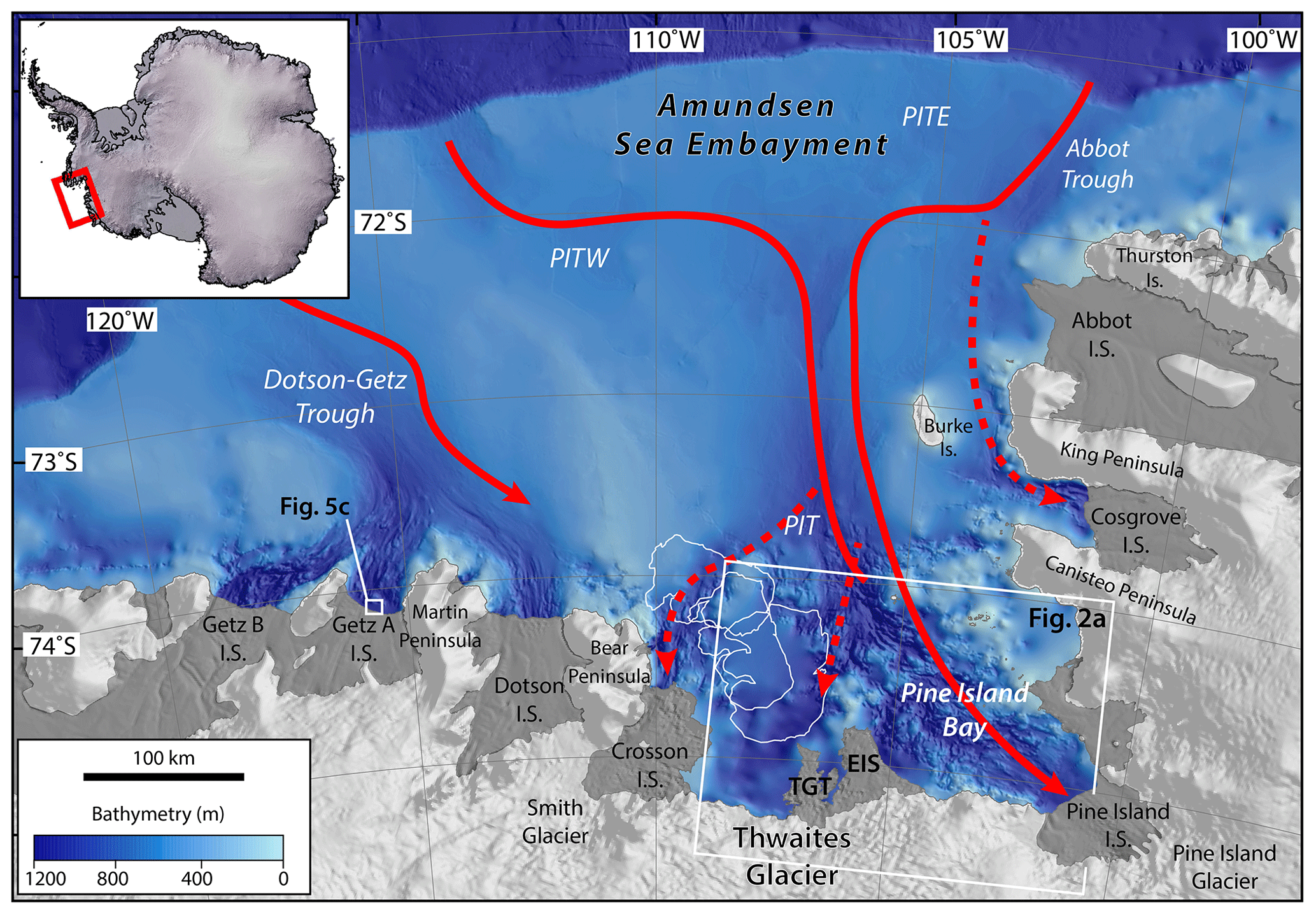
Figure 1Regional bathymetry for the Amundsen Sea Embayment and location of Thwaites Glacier (TG), West Antarctica. Bathymetry is from IBCSO (Arndt et al., 2013); arrows show observed (solid) and inferred (dashed) pathways for CDW across the continental shelf towards the grounding zones of Pine Island, Thwaites and Smith glaciers (following Nakayama et al., 2013; Dutrieux et al., 2014) and along the Dotson–Getz trough (Ha et al., 2014). PIT is Pine Island Trough; PITE is Pine Island Trough East; PITW is Pine Island Trough West; TGT is Thwaites Glacier Tongue; EIS is Eastern Ice Shelf; other ice shelves (I.S.) are also labelled. White outlines north of TG are mapped positions of the B-22A iceberg from 2002, 2010 and 2018, from south to north. Note the more blurry look of the bathymetry in front of TG (in IBCSO this bathymetry is based on the Tinto and Bell, 2011, gravity inversion and interpolation), where ship access has been hampered before austral summer 2018/2019 by persistent fast ice and the presence of the B-22A iceberg.
At present, the eastern and central parts of TG are fronted by two protruding floating ice masses, the Eastern Ice Shelf (EIS) and the Thwaites Glacier Tongue (TGT), which extend for 40–50 km beyond the grounding zone, to the west of which a 20 km wide mélange of icebergs and sea-ice exists (Fig. 2). For simplicity, we shall refer to these floating ice masses collectively as the Thwaites Ice Shelf (Fig. 2a; see Heywood et al., 2016). The TGT extends from the fastest-flowing region of TG (Fig. 2a) and has, on multi-decadal timescales, advanced up to 130 km from the grounding zone before the majority of the floating tongue has calved (MacGregor et al., 2012). As a result, marine areas beyond this have been rendered inaccessible by remnants of the TGT as they have drifted north-northwest, including the very large B-10 and B-22A icebergs that remained grounded on the continental shelf for decades after they had calved before 1965 and in 2002, respectively (Fig. 1) (Ferrigno et al., 1993; Rabus et al., 2003; MacGregor et al., 2012). In contrast, the EIS remains pinned on a sea-floor high that restricts its flow (Rignot et al., 2001; Tinto and Bell, 2011; Jordan et al., 2020) and induces shear between the EIS and TGT. Satellite imagery confirms that since 2006 increased crevassing and fracturing has weakened the shear zone between the EIS and TGT (Kim et al., 2015), with the two ice shelves remaining connected until 2010 (MacGregor et al., 2012). Due to its inaccessibility, few marine observations have been made on the inner continental shelf in front of TG (Jacobs et al., 2012). The existing oceanographic data, along with more comprehensive results from Pine Island Bay, confirm the presence of CDW in the deep troughs east and north of the EIS (Dutrieux et al., 2014; Jenkins et al., 2016) and identify these troughs as potential pathways for warm water to the TG grounding zone (Fig. 2a; Milillo et al., 2019).
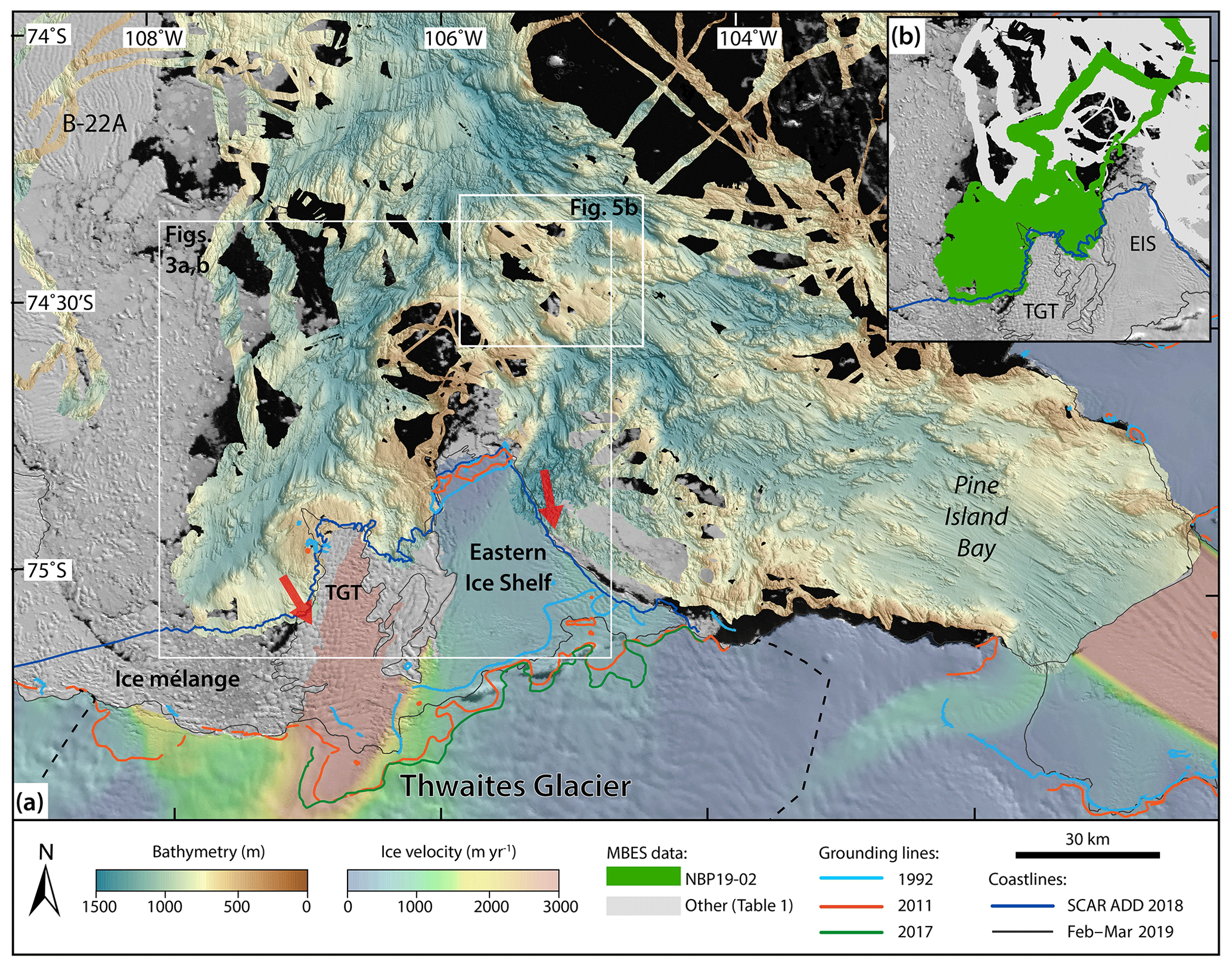
Figure 2(a) New MBES grid for the inner Amundsen Sea Embayment. Ice-velocity data from the MEaSUREs V2 dataset (Mouginot et al., 2019); grounding lines for 1992 and 2011 are from Rignot et al. (2011) and that for 2017 is from Milillo et al. (2019); red arrows delineate CDW pathways following Dutrieux et al. (2014) and Milillo et al. (2019). The black dashed line marks the boundaries of the drainage basin of Thwaites Glacier (Vaughan et al., 2001). (b) NBP19-02 data coverage versus other MBES datasets (Table 1). The dark blue coastline illustrates the ice-shelf and ice mélange extent during survey on NBP19-02 and was digitised from Landsat 8 imagery.

Figure 3(a) High-resolution bathymetry map of the inner Amundsen Sea shelf in front of TG and the adjacent part of Pine Island Bay showing the large-scale sea-floor morphology including bathymetric troughs (Thwaites Trough, T2–T4; main axes highlighted by black dashed lines) and highs (H1–H3) that form a broad NNE–SSW ridge continuing into a ridge further offshore in Pine Island Bay, northeast of the Eastern Ice Shelf (white dashed line). (b) Mapped sea-floor landforms; streamlined features show the former flow direction of an expanded TG (white arrows). (c) Cross-sectional profiles of the bathymetric troughs; locations of profiles in (a).
Regional bathymetric compilations for the ASE shelf use multibeam echo-sounder (MBES) data where available in offshore regions (Nitsche et al., 2007, 2013; Arndt et al., 2013), with gravity inversions and a limited amount of echo-sounding data from autonomous underwater vehicles (AUVs) for sub-ice-shelf cavities (Jenkins et al., 2010; Tinto and Bell, 2011; Millan et al., 2017; Jordan et al., 2020). These datasets have identified glacially modified depressions on the continental shelf that act as conduits for CDW transport towards present-day ocean-terminating glacier margins in the ASE (Fig. 1) (e.g. Nitsche et al., 2007; Walker et al., 2007; Jacobs et al., 2012; Nakayama et al., 2013). Landward of the MBES data coverage that existed prior to this study, gravity inversions had indicated the presence of a NE–SW-trending ridge on which the EIS is pinned (Rignot, 2001; Tinto and Bell, 2011; Millan et al., 2017). Millan et al. (2017) reported that the ridge is interrupted by at least three channels with water depths between 600 and 1000 m, interpreted to be potential CDW pathways towards the grounding zone.
Considering the use of sea-floor bathymetry at higher spatial scales (than regional compilations), the analysis and interpretation of submarine glacial landforms revealed by MBES datasets provides important information on the dynamics and configuration of former glaciers and ice sheets. On the inner ASE shelf, for example, the bed of an expanded PIG has revealed the past flow direction of a large ice stream that extended more than 400 km to the continental shelf break (Evans et al., 2006; Graham et al., 2010; Jakobsson et al., 2012), as well as evidence for extensive erosion by subglacial water during past glaciations (Nitsche et al., 2013; Kirkham et al., 2019). These offshore areas also contain well-preserved information on the form and composition of the former ice-sheet bed that may, by analogy, shed light on basal conditions under the modern ice sheet (e.g. Clark et al., 2003; Ó Cofaigh et al., 2005). The roughness of an ice-sheet bed, or its variation in the vertical over a certain horizontal distance, is a primary control on basal drag, and therefore ice-flow velocity, and can be analysed for past ice-sheet beds from MBES datasets (offshore) or from satellite-derived digital elevation models (onshore) (e.g. Falcini et al., 2018). Even small (metre-scale) obstacles on the bed have been shown, theoretically, to exert critical basal drag on an overlying ice mass (e.g. Nye, 1970; Schoof, 2002). The great value in analysing MBES datasets for this purpose lies in their higher-resolution and even two-dimensional spatial coverage when compared with radar or seismic-reflection data acquired in over-ice studies (Spagnolo et al., 2017). Previous roughness analyses (from contemporary ice-sheet beds) have associated fast-flowing ice with smoother beds (e.g. Siegert et al., 2004; Rippin et al., 2011); however, recent papers acknowledge that the picture is likely to be much more complex than this with observations of fast flow occurring over even hard, rough beds, including at TG (Schroeder et al., 2014), and acknowledging that processes acting at a variety of spatial scales (including erosion and deposition) will affect spatially varying bed conditions and roughnesses (Jordan et al., 2017; Falcini et al., 2018).
Here, we present the first direct observations of sea-floor bathymetry adjacent to Thwaites Ice Shelf acquired as part of the first International Thwaites Glacier Collaboration (ITGC) cruise on RV/IB Nathaniel B. Palmer in January–March 2019 (cruise NBP19-02). In the first part of the paper, we use these data to investigate the character (bed geometry and substrate composition) of topographic highs that were former grounding zones and ice-shelf pinning points as well as to better resolve sea-floor troughs as potential modified CDW pathways to the modern Thwaites grounding zone. In the second part of the paper, we investigate the roughness characteristics of this palaeo-glacier bed as a potential analogue for the current bed of TG, and we relate flow-line roughness to the drag contribution of an overriding ice mass. We compare bed roughnesses and basal drag contributions from bathymetric profiles from the inner ASE shelf to bed profiles from upstream areas of PIG and TG, as well as to a smooth palaeo-ice-stream bed offshore the nearby Getz A Ice Shelf. To reflect these two components of the paper we describe (1) the observational (geophysical) datasets used and interpret the new bathymetric dataset, which is also provided as a publicly available stand-alone grid; and (2) the spectral approach and how we use it to quantitatively examine the roughness and basal drag contributions from former and modern TG beds. We use sea-floor landform evidence to describe both the flow of an expanded TG over the area as well as the spatial variability in bed composition over a series of topographic highs that once acted as both the grounding zone for TG and as pinning points for its ice shelf. We demonstrate that the offshore area just seaward of Thwaites Ice Shelf is an appropriate analogue for the modern grounding zone of TG, both in terms of its bed characteristics and in the effect of its rugged bed topography on ice flow, by calculating drag contribution for different scales of roughness. Finally, we highlight the importance of high-resolution MBES observational data for constraining gravity inversions and regional bathymetry compilations, which are essential boundary conditions for predictive numerical modelling experiments and for accurately calculating the flux of warm water to the grounding zone.
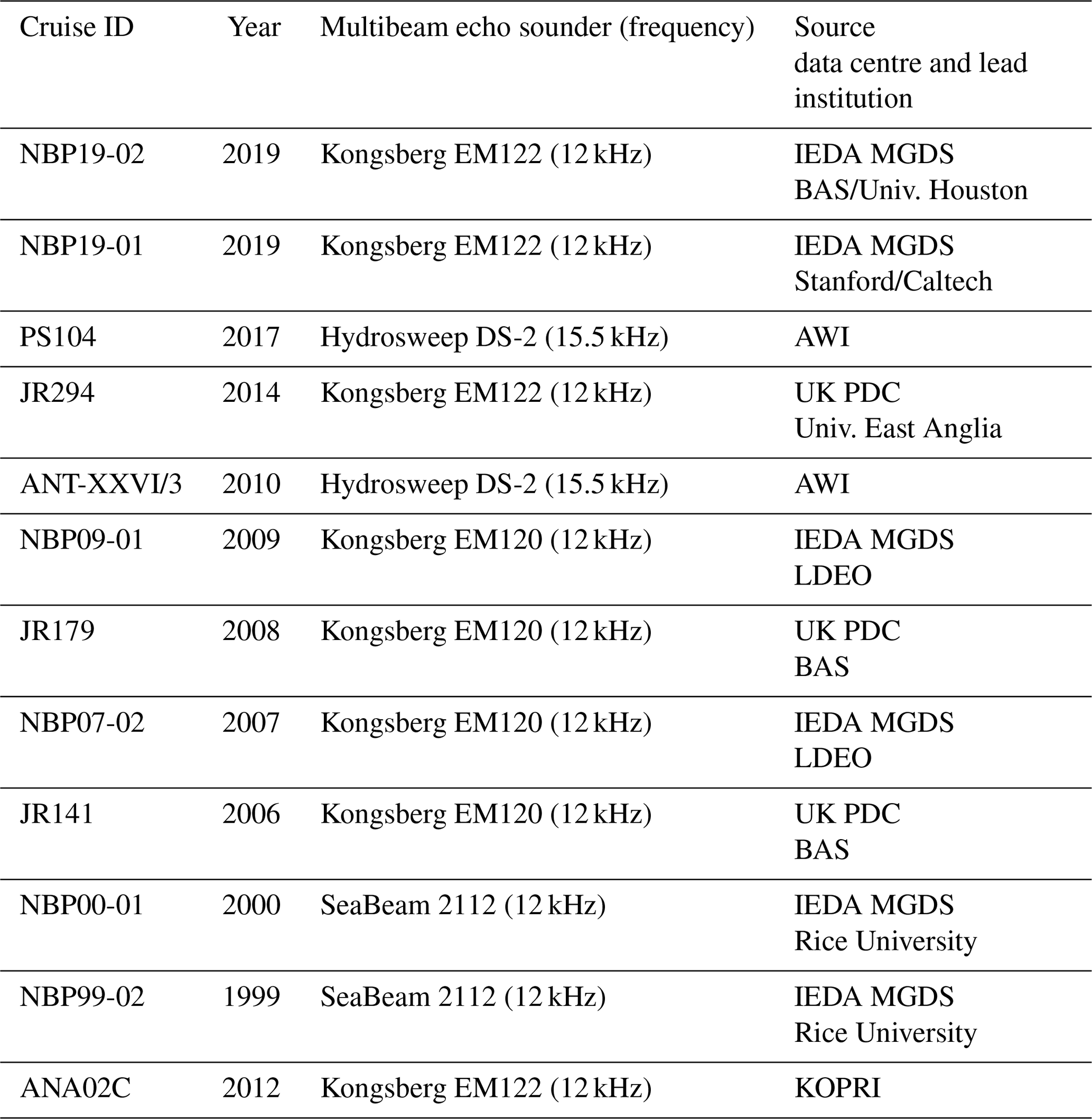
During ITGC cruise NBP19-02, the marine areas in front of TG were unusually clear of sea ice and icebergs, providing a unique opportunity for bathymetric data acquisition at the margin of Thwaites Ice Shelf (Larter et al., 2020). MBES data were acquired using a hull-mounted Kongsberg EM122 echo sounder with 288 across-track beams and an operational frequency in the range 11.25–12.75 kHz. Navigation information and vessel motion information, used to correctly locate depth measurements in real time, were taken from the ship's Seapath 330, a combined GPS and motion reference unit. The MBES was configured with “high-density equidistant” beam spacing, meaning that more than one sounding can be produced per beam (up to 432), effectively increasing across-track resolution, and in “dual-ping” mode, which ensures equal across- and along-track sounding spacing. As an example, in 600 m water depth with maximum port and starboard beam angles set at 60∘ from nadir (typical conditions and settings on NBP19-02), this results in a sounding spacing on the sea floor of ∼5–7 m; in 1200 m water depth (near maximum survey depths during NBP19-02) this sounding spacing would effectively double to 10–14 m. Here, in addition to this new dataset, we have compiled all available MBES data in the area from UK, US, German, Swedish and Korean expeditions (Table 1; Fig. 2) to produce gridded bathymetric data products. Note that the sounding spacing achievable by each MBES system varies considerably depending on the system setup, with older systems generally attaining lower spatial resolution. For example, at 1200 m water depth and maximum beam angles 60∘ each side of nadir, the Kongsberg EM120 MBES would achieve an across-track sounding spacing of only 22 m and the SeaBeam 2112 MBES only 35 m. Together, these two systems were responsible for acquiring data from five cruises in the area (Table 1).
Table 1Research cruises that acquired MBES data used in this compilation. IEDA MGDS is the Interdisciplinary Earth Data Alliance Marine Geoscience Data System (USA; http://www.marine-geo.org/index.php, last access: 21 January 2020); UK PDC is the United Kingdom Polar Data Centre (UK; https://www.bas.ac.uk/data/uk-pdc/, last access: 21 January 2020); BAS is the British Antarctic Survey; AWI is the Alfred Wegener Institute (Germany); LDEO is the Lamont-Doherty Earth Observatory of Columbia University; KOPRI is the Korea Polar Research Institute.
For NBP19-02, data processing was performed on board using MB-System (Caress and Chayes, 1996; Caress et al., 2020) in order to apply optimal sound velocity profiles (SVPs) to each data file and to remove erroneous soundings. Ray tracing and sea-floor depths were calculated using SVPs generated from conductivity–temperature–depth (CTD) and expendable bathythermograph (XBT) casts made during NBP19-02 (Larter et al., 2020). Most of the other bathymetry datasets were also initially ping edited during each respective cruise; however, minor additional cleaning was performed in MB-System and QPS Fledermaus (Mayer et al., 2000) after the datasets were collated when clear outliers could be easily identified. Ultimately, and to accommodate the different resolutions of the original datasets, the bathymetric sounding data were gridded in MB-System using a Gaussian weighted mean filter algorithm to produce an isometric 50 m digital elevation model (DEM) for the sea floor on the southern ASE shelf. A degree of interpolation was applied to the final grids in data gaps only, filling areas six cell widths away from cells with real soundings, i.e. for a 50 m grid interpolation will fill cells up to 300 m away from a cell with real soundings. A lower-resolution DEM (500 m grid cells) was produced for studies that typically use coarser bathymetric information. Together, the 50 and 500 m DEMs are presented as a stand-alone regional mid-resolution bathymetric dataset (Hogan et al., 2020) In addition, in order to examine the nature of specific sea-floor features (e.g. ice-shelf pinning points), higher-resolution grids (30 m grid cells) were produced where sounding densities allowed (e.g. Fig. 4). Final grids were visualised and analysed in QPS Fledermaus 7.8.6 and ArcGIS 10.6. Sea-floor trough and channel metrics (including widths, depths, symmetry, form ratio, u-/v-shape characterisation) were derived using the methods described in Kirkham et al. (2019); the reader is referred to Fig. 2 of Kirkham et al. (2019) for a graphical depiction of the channel metrics measured.
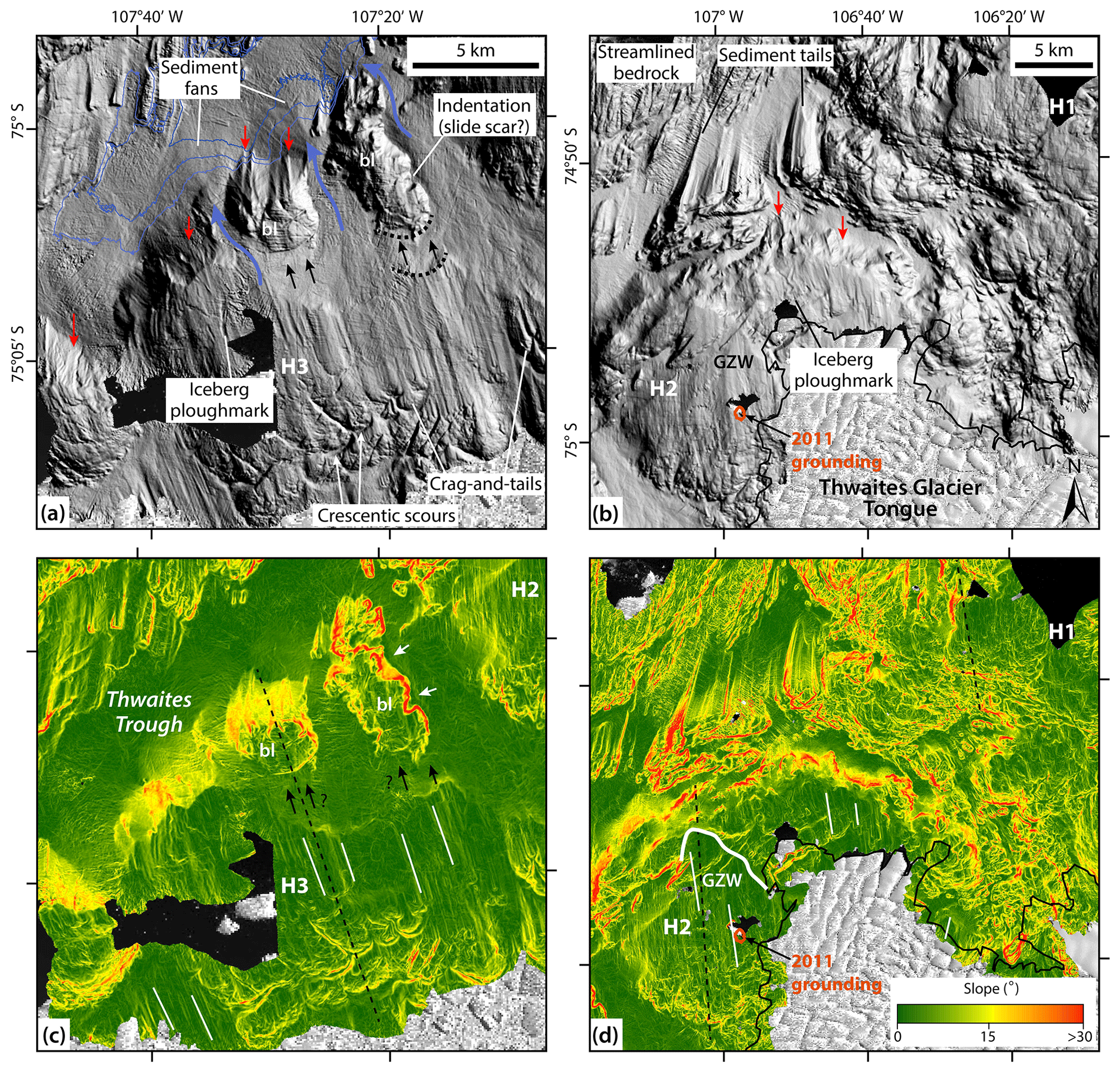
Figure 4Detailed maps of the MBES data and their first derivative and slope over the sea-floor highs in front of Thwaites Glacier. Panels (a) and (c) show the H3 high. Panels (b) and (d) show the H2 high and western flank of H1. Red arrows in (a) and (b) point to gullies incised into the seaward flanks of the highs; the white lines in (c) and (d) mark glacial lineations; bl shows the isolated blocks of H3, and black arrows in (a) and (c) denote their possible transport paths, with the black dotted lines in (a) illustrating semicircular indentations; white arrows in (c) point to a channel at the base of one of the blocks; blue arrows in (a) indicate the downslope transport direction of material into sediment fans at the front of H3 highlighted by bulges in the contours (contour levels 1100, 1125 and 1150 m). Black dashed lines in (c) and (d) locate the profiles in Fig. 5a. GZW is grounding-zone wedge.
Our bathymetric compilation includes more than 2000 km2 of new MBES data between the EIS and the TGT and west of the TGT that provides near-continuous bathymetric coverage for ∼40 km north of the present-day ice-shelf margin (Figs. 2, 3). Data gaps remain in the western part of the area in front of the ice mélange, east of Crosson Ice Shelf, as icebergs and bergy bits released from the ice mélange persistently covered this region during NBP19-02. In addition, perennial fast ice and huge icebergs, such as the 80 km long and 45 km wide iceberg B-22A, that calved periodically from the TGT and then moved slowly north- and northwest, thereby episodically running aground, have generally prevented survey between TGT and Crosson Ice Shelf (see area with B-22A outlines in Fig. 1).
The sea-floor bathymetry offshore Thwaites Ice Shelf is dominated by an elongate depression oriented NNE–SSW (Thwaites Trough) and a series of topographic highs (H1-H3) along its southern margin (Fig. 3a). The depression is characterised by water depths of 1100–1250 m, which is 200 to 400 m deeper than the sea floor on its flanks; it typically has a relatively flat or gently inclined floor (Fig. 3a, c). Although the depression appears to be continuous for at least 75 km, and connects with areas of deep (>1300 m) sea floor directly north of the EIS and in Pine Island Trough further east (Fig. 2a), its width varies significantly along its length and the flanks are discontinuous in form. As a result, we do not define this feature as a channel, which implies incision by water flow, but rather as a small trough. The topographic highs that make up the southern flank of the trough (H1-H3) decrease in height (above the surrounding sea floor) from NNE to SSW and appear to form a broad (>15 km) but discontinuous ridge, also oriented NNE–SSW. The large, discontinuous ridge is the extension of a bedrock ridge in Pine Island Trough to the east that has the same orientation (Figs. 2, 3a; Nitsche et al., 2013). The most prominent high (H1) occurs immediately north of the EIS with a shallowest recorded water depth of just 82 m and extends at least 40 km in a north–south direction. The northern part of the EIS is pinned, about 45 km downstream of the grounding zone (Rignot et al., 2001; Tinto and Bell, 2011; MacGregor et al., 2012), on the southern part of this high, forming an ice rumple in the EIS (Matsuoka et al., 2015). The shallowest water depths on the two highs H2 and H3 (from NNE to SSW) are 362 and 611 m, respectively. Indeed, a pinning point for TGT on H2 has been identified from remote-sensing data (Rignot et al., 2011), but the TGT must have fully retreated from that point prior to NBP19-02. North of the trough and ridge (north of S) is an area of rugged morphology characterised by shallow sea-floor ridges and deep basins (>1400 m); this area merges with similar terrain in Pine Island Trough described by Nitsche et al. (2013) as their “area 2” (Fig. 2). East of the EIS, the eastern flank of H1 is just exposed but the bathymetry is dominated by a deep (1000–1200 m), rugged area of sea floor, bounded on its eastern edge by a bedrock high in Pine Island Bay that continues southeastwards towards the grounding zone (Fig. 2a). The deepest part of this area appears to form a poorly defined bathymetric trough oriented NNE–SSW (T4; Fig. 3a); oceanographic measurements and models confirm that this deep acts as a pathway for CDW towards grounding lines in western Pine Island Bay (Fig. 2a) (Dutrieux et al., 2014; Nakayama et al., 2019).
3.1 Glacial landforms
The large-scale morphology of the sea-floor offshore Thwaites Ice Shelf is overprinted by linear features oriented subparallel to the trough and ridge. Streamlined subglacial landforms occur in areas where bedrock crops out at the sea floor, either on topographic highs or interrupting the smooth trough floor or rugged basin floors (Fig. 3a, b). These features are identified as crag and tails by their tapering form and are 750–4000 m long, 200–2000 m wide and 25–250 m high (Figs. 3, 4, S1a in the Supplement), as well as their morphological similarity to crag and tails from other deglaciated terrains (e.g. Dowdeswell et al., 2016; Maclean et al., 2016; Nitsche et al., 2016). The wider southern ends of the crag and tails are rugged and have significant relief, suggesting bedrock composition, whereas the northern ends are smooth and elongate, indicative of a sedimentary composition. These landforms are produced subglacially as glacier ice flows across bedrock obstacles producing the characteristic morphology through erosion and deposition (Benn and Evans, 2010; Nitsche et al., 2016). The tapering of these features north-northeastwards indicates palaeo-ice flow of TG in this direction towards Pine Island Trough (Fig. 3b); east of the EIS the orientation of these landforms varies from N–S to NW–SE, depicting flow around the H1 high (Fig. 3b). Curved or semicircular moats – crescentic scours (Lowe and Anderson, 2003; Graham et al., 2009; Graham and Hogan, 2016) – occur around the southern (upstream) sides of some crag and tails (Figs. 3b, 4a, S1d) and are suggestive of erosion by meltwater or, alternatively, a till slurry or mobile basal ice, upstream of bedrock obstacles (see Graham and Hogan, 2016). On the H2 and H3 highs, subtle elongate ridges separated by linear grooves also occur (Fig. 3a). These glacial lineations have parallel sides; lack a pronounced and wider end; and are 1000–2500 m long, 100–200 m wide and 2–10 m high; their crest-to-crest spacing is typically 200–500 m (e.g. Fig. S1b). These features, which were produced subglacially, have relatively short elongation ratios () and are oriented parallel to crag and tails also on the tops of the highs but are slightly oblique to crag and tails in the trough (Fig. 3). A distinct but discontinuous scarp is mapped on the top of the H2 high, upstream from its frontal edge (Figs. 3, 4b, d). The scarp has a curved planform and a steep (3–4∘) northern and gentle (0.5∘) southern slope; glacial lineations occur on the gentle back-slope of this feature which extends for about 15 km in a SW–NE direction. The asymmetric geometry and lineated back-slope of this landform identify it as a grounding-zone wedge (GZW; Fig. S1c) (Alley et al., 1989; Larter and Vanneste, 1995; Dowdeswell and Fugelli 2012; Jakobsson et al., 2012), i.e. a wedge of sedimentary material that built up at the grounding zone when it was stable for a time on the H2 high. This feature is interrupted, however, by a ∼40 m deep groove or small channel with bedrock ridges visible on either side, suggesting that the sedimentary wedge is not thick enough to fully bury the underlying topography; i.e. it is only tens of metres thick. Discrete 6–10 m deep linear to curvilinear furrows with small berms (4–6 m) were mapped on H3 and north of the GZW front scarp (Fig. 4a, b); these are interpreted as iceberg plough marks.
Sea-floor highs in the area are also variously gouged and streamlined, resulting in a pattern of grooves and bedrock ridges (Fig. S1e). Grooves on the H1–H3 ridges occur on their southern (upstream) parts and exhibit a range of orientations that probably relate to the structure of the underlying bedrock exploited by glacial erosion. The grooves are typically <20 m deep, <200 m wide and <6000 m long. The surfaces of sea-floor highs north of the H1–H3 ridge have a more streamlined appearance resulting from shallow, semi-parallel shallow grooves that are preferentially aligned with the crag and tails (Figs. 2, 3). Streamlined bedrock highs of this type are typical of inner-shelf morphologies around Antarctica (e.g. Wellner et al., 2006; Livingstone et al., 2013) including in the adjacent eastern part of Pine Island Bay (Nitsche et al., 2013). Taken together, the orientations of the streamlined subglacial landforms (crag and tails, glacial lineations, bedrock grooves/ridges) define the former ice-flow directions of an expanded TG (depicted by white arrows in Fig. 3b), confirming that this area is the former bed for grounded glacier ice.
3.2 Trough and channel metrics
Multiple bathymetric troughs and bedrock channels were mapped and analysed in the area beyond Thwaites Ice Shelf as part of this study (Fig. 3a). Troughs and channels in the adjacent part of Pine Island Bay have been described comprehensively by Nitsche et al. (2013) and Kirkham et al. (2019). The larger troughs in our study area, which have also been identified on gravity-derived regional bathymetry maps (Millan et al., 2017; Jordan et al., 2020), are considered important as potential pathways for the transport of CDW towards the grounding zone of TG and warrant full description here. We distinguish these comparatively larger troughs, based on their size, connectivity and variable flank form (as described above), from the channels which are notably smaller in scale (Fig. S2). The latter have continuous, parallel-sided flanks and undulating thalwegs and incise into rugged sea-floor areas interpreted as bedrock (e.g. Fig. S1e). It is widely accepted that channels of the latter type were eroded by pressurised subglacial water flow (Lowe and Anderson, 2003; Nitsche et al., 2013; Kirkham et al., 2019), whereas the troughs likely relate, at least in part, to underlying geological structures such as dykes and tectonic deformations (see Gohl et al., 2013) that have been variously modified by ice, as well as possibly by subglacial water flow.
Cross-sectional analyses of the troughs (n=166) reveal their large scale, with average widths, depths and cross-sectional areas being 2090 m, 90 m and 144 000 m2, respectively (Fig. S2). The troughs are typically 10–30 times as wide as they are deep, although we note that there is a significant size difference between the main NE–SW trough (Thwaites Trough) and the remaining troughs (Figs. 3a, S2). By comparison, the bedrock channels (n=822) are on average 520 m wide, 50 m deep with a cross-sectional area of 18 000 m2. The channels are generally 5–10 times wider than they are deep. The derived b values, which characterise cross-sectional shape (Pattyn and Van Huele, 1998), suggest that the bedrock channels are between v and u shaped, whereas the larger troughs have no dominant cross-section shape (Fig. S2). In general, the trough floors are flat or inclined in cross profiles (Fig. 3c) and are gently undulating in along-trough profiles.
The main Thwaites Trough is oriented NNE–SSW, which is oblique to the northerly palaeo-ice-flow directions immediately in front of Thwaites Ice Shelf (Fig. 3b). This indicates that, at the time that the subglacial landforms were produced, ice was thick enough not to be fully steered by even major elements of the bed topography. The two southernmost troughs that we have analysed (T2 and T3 in Fig. 3a) are oriented perpendicular to Thwaites Trough (i.e. NNW–SSE), and the troughs north and east of the EIS are generally aligned with palaeo-ice-flow directions (Figs. 2, 3a). Note that the T1 trough is not well covered by our MBES dataset and is not discussed in detail here. The T2 and T3 troughs, whose floors have water depths of 800–900 m, separate the H1–H3 bathymetric highs and are of interest as potential pathways for CDW to the TG grounding zone. Long profiles from the T2–T4 troughs (Fig. S3) identify sill depths along the pathways of the troughs that may act as important pinch points for ocean circulation, in particular if they impede CDW inflow towards the Thwaites grounding zone (cf. De Rydt et al., 2014). T2 has a smooth long profile with a prominent sill at 710 m depth at about W, S, whereas T3 has a rugged profile with three bathymetric sills in its northern (ice distal) part with depths of 750–760 m, as well as several other sills further south (ice proximal) around 780 m water depth (Fig. S3a). The bathymetry around T4, east of the EIS, is generally deeper (>1000 m) than most of T2 and T3, so the main constriction on this trough seems to be where it crosses the NE–SW-trending sea-floor ridge in Pine Island Bay (Fig. 2a). At this location, around W, S, there is a sill at 880 m depth (Fig. S3d). Channel widths at these locations are 5000 m for the T3 sills and 2500 m for the T4 sill (although this is not the only interruption in the ridge in Pine Island Bay). Widths were measured at 500 m depth as this is taken to be a reasonable top-CDW depth for the area (based on oceanographic measurements; Bastien Queste, personal communication, 2020). The bathymetry of the highs west of T2 is >500 m depth, meaning that CDW could effectively flood over this topography rather than be constrained to the trough; however, if it was topographically routed (see Nakayama et al., 2019) through T2, then the channel width at the sill is 4700 m (at 640 m water depth).
3.3 Bathymetric highs and ridges
Owing to the importance of sea-floor highs in front of the Thwaites Ice Shelf as barriers to CDW inflow, and as former ice shelf/sheet pinning points, we examine the morphology of the discontinuous NNE–SSW-trending ridge in detail (Fig. 4). The ridge comprises the H1–H3 highs separated by the two troughs described above (T2 and T3; Fig. 3a). The width of the ridge varies significantly, from 6 km in the SW of the study area to at least 40 km over H1, although we acknowledge that data coverage is limited. In some places, the bathymetric highs are strikingly flat topped. These planar features are accentuated in maps of the first derivative of bathymetry, slope, which reveals both low slopes (<2∘) (Fig. 4c, d) and low roughness over H2, H3 and the western part of H1. The continuation of the ridge further north into Pine Island Trough has a similar surface expression but is generally narrower (Fig. 3a). These areas with low surface slopes are atypical when compared with other bathymetric highs in the area, which have rugged surface morphologies characterised by bedrock grooves and channels (Figs. 2, 4d) (Nitsche et al., 2013; Arndt et al., 2018; Kirkham et al., 2019). Instead, the low slope values are similar to those derived for the base of the troughs in front of Thwaites Ice Shelf (Fig. 4a) and the sediment-filled basins just seaward of the Pine Island Ice Shelf front (Nitsche et al., 2013; Kuhn et al., 2017). At least two distinct levels of flat-topped surfaces occur at 400 and 640 m water depth (Fig. 5). We suggest that this morphology was generated as the highs were overridden and eroded by a formerly expanded TG and Thwaites Ice Shelf (with the necessary ice thickness to reach the depth of the flat-topped surfaces). A value of ∼400–500 m is similar to ice-shelf thicknesses for Thwaites Ice Shelf today (Griggs and Bamber, 2011; Jordan et al., 2020), and a prevalence of flat-topped highs at this depth may, therefore, support recent modification of the sea-floor highs at TG. In contrast, the deeper flat top of H3 (640 m depth) was probably formed at an earlier stage, as was the flat top of the high in Pine Island Trough, as that area is known to have been ice-free (sheet and shelf) for at least the last 10 kyr (e.g. Kirshner et al., 2012; Hillenbrand et al., 2013). The interpretation of erosion or planing off by an ice shelf is supported by the occurrence of glacial lineations on the tops of the highs (Fig. 3b), which are in line with modern ice-velocity vectors (Mouginot et al., 2019) but oblique to the orientation of crag and tails in the troughs, thus indicating a change in flow direction from grounded ice flow to ice-shelf flow over the high. A similar interpretation was made for the lineated surface of a former pinning point of the Pine Island Ice Shelf (PIIS) that has been recently exposed by ice-shelf calving events (Arndt et al., 2018), although that feature was not planed off to form a flat-topped high but rather has a stepped and rugged surface morphology albeit with some gently sloping parts (see their Fig. S3). We note, however, that alternative explanations are possible for this morphology, namely that the flat tops are an inherited feature produced by erosion down to horizontal bedrock strata or that rugged bedrock highs, which are typical of the inner Amundsen Sea shelf (see Nitsche et al., 2013), were mantled by some thickness of glacigenic material that levelled the topography below. The former is relatively easy to discount accepting that the inner shelf of the ASE is composed of crystallite basement with seismic-reflection profiles showing that northward-dipping sedimentary strata only occur on the middle and outer shelf (see Graham et al., 2009; Gohl et al., 2013). In this setting close to the current TG grounding zone, it is perhaps easier to conceive of the latter explanation that rugged bedrock features were mantled by glacigenic material delivered to the area when the grounding zone was located on or near the highs and then flattened by some degree of glacial compaction and/or erosion as it was overtopped by TG and the subsequent Thwaites Ice Shelf. This is consistent with our suggestion for the formation of these flat tops as we cannot tell from our data either what sediment thickness occurs on the highs or how much erosion took place, and we acknowledge that the amount of ice-shelf erosion may have been small, only skimming unconsolidated material from the surface of the highs. The presence of GZWs and glacial lineations on the highs, and sub-bottom profiler data (Fig. S4), confirms that at least some thickness of unconsolidated material occurs on the highs, but seismic-reflection profiles would be required to fully capture the internal structure of these features.
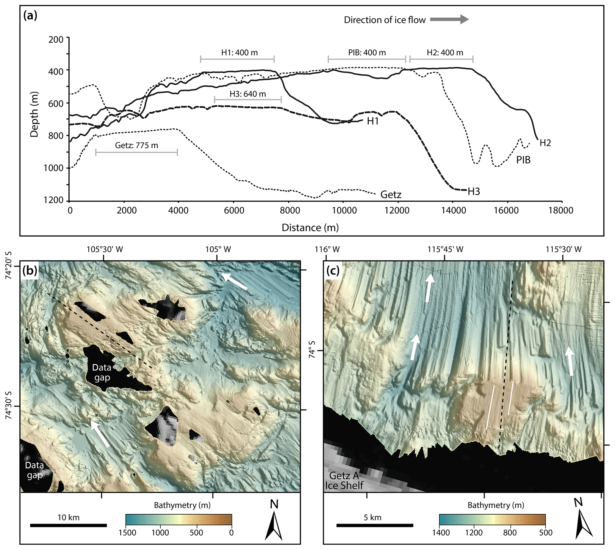
Figure 5Flat-topped highs in the Amundsen Sea. (a) Cross-sectional profiles over H1–H3 highs at Thwaites Glacier (for location of profiles, see Fig. 4c, d), further offshore in Pine Island Bay (PIB; location of high in Fig. 2a, location of profile in Fig. 5b) and offshore from the Getz A Ice Shelf (location of high in Fig. 1; location of profile in Fig. 5c), showing sea-floor highs planed off at different depth levels. The flat portions of the profiles are marked with grey bars and the depth elevation for that flat top given above, so “H1:400 m” means the flat part of the profile over H1 high is at 400 m water depth. (b) MBES of flat-topped highs part of the discontinuous sea-floor ridge in PIB. (c) MBES of a flat-topped high with glacial lineations (white lines) just in front of the Getz A Ice Shelf (following Nitsche et al., 2016). White arrows show direction of past ice flow based on streamlined subglacial landforms.
No matter the exact formation mechanism, the flat-topped morphology of the highs in our study area is striking and notably rare for sea-floor highs around Antarctica. We note a similar but less pronounced terrain over some highs along the same structural ridge in Pine Island Bay, i.e. east of the EIS (Fig. 5b), and a solitary very flat topped high, with comparable dimensions to those offshore TG, is visible <5 km north of the Getz A Ice Shelf (Fig. 5c). Beyond these rare examples, the best analogy for this morphology probably comes from a set of “iceberg terraces” on terminal moraines at the mouth of a Svalbard fjord, which display remarkably flat topped surfaces at several bathymetric levels. These are interpreted to have formed as tabular, flat-based icebergs overtopped and eroded morainal sediments (Noormets et al., 2016). It should be noted, however, that sediments of this morainal bank complex probably consist of unconsolidated material that has not been overridden (or compacted) by grounded ice, meaning that they are likely more erodible than basement highs in front of Thwaites Ice Shelf. Nevertheless, the flat-topped morphology is suggestive of a sedimentary cap on the pinning points at TG, and the fact that similar features exist in Pine Island Bay and beyond the Getz A Ice Shelf may indicate that pinning points with such sedimentary caps are widespread on the inner shelf in the Amundsen Sea.
New geomorphic information is also revealed by the flanks of the highs (Fig. 4a, b). The northern (ice distal) flanks of the H2 and H3 highs are characterised by subtle downslope-trending gullies that transition into a smooth but inclined sea floor in the troughs at a distinct break of slope. There are also a few, discrete semicircular indentations in the scarp between the surface of the highs and their flanks (Fig. 4a). The gullies have simple non-branching geometries, have small dimensions (widths 150–700 m, depths 5–50 m, lengths <2 km), and typically define broad u shapes in cross section, although some v-shaped forms are present. In addition, their form is consistent with other Antarctic submarine gully systems (e.g. Fig. S1f; Gales et al., 2013; Post et al., 2020). Thus, we interpret the gullies as the result of the downslope mass movement of material from the tops and sides of the H2 and H3 highs via gravitational processes into the small sediment fans at the base of the slope (Fig. 4a). The semicircular indentations may be the headwalls of small slide scars (cf. Noormets et al., 2009; Gales et al., 2013). One 6 km by 2.6 km segment of the H3 high is somewhat detached from other parts of the ridge and appears particularly fragmented on its flanks (Fig. 4a). About 1500 m south of this, on the main H3 high, is a distinct break in slope with the same planform shape as the back of the detached segment that we refer to as a “block” (bl in Fig. 4a, c). Similarly, 2 km west of this block is another somewhat isolated 3 km by 1.8 km block of H3 that is incised by gullies on its northern front and lacks lineations on its surface (Fig. 4a). We consider several interpretations for these features. First, it is possible that they are detached blocks of the H3 high that had been displaced downslope over a short distance (black arrows in Fig. 4a, c), remaining largely intact, but subsequently affected by some gravitational collapse of their flanks. Slide megablocks with similar dimensions (or larger), non-crystalline compositions and degraded flanks are known from, for example, the Hinlopen Slide scar on the northern Barents Sea margin (Vanneste et al., 2006; Hogan et al., 2013). The second possibility is that the blocks are small bedrock highs that have been variously mantled by and surrounded by glacigenic sediment, either deposited subglacially on their surfaces or as it was transported downslope by gravity-driven processes (towards the sediment fans) from the H3 high (see blue arrows in Fig. 4a). If the latter case is true, then the pronounced semicircular indentation on the eastern block (labelled in Fig. 4a) may be an erosional scour mark formed by the recurrent flow of water, as is evidenced by the small channel on the eastern side of the block (white arrows in Fig. 4c).
4.1 Spectral analysis of bed roughness
The idea that the drag experienced by a glacier can be analysed by treating the basal roughness as a superposition of sine waves of different wavelengths (λ) has a long history in glaciology (e.g. Nye, 1970; Kamb, 1970; Hubbard et al., 2000). In these approaches, Fourier methods are used to find the drag contributed by roughness that falls within some range of wavelengths (or band of spatial frequencies). More recently, a similar approach has treated the longer wavelength undulations that can affect flow near the upper surface of the ice (Schoof, 2002). Knowledge about the power spectrum of the basal roughness is an essential input to all of these studies.
The high-resolution bathymetric grid that we have produced (Fig. 2) represents the former beds of expanded TG and PIG. As such, it contains information about bed geometry and roughness that can be used to investigate the behaviour of glacier ice over this terrain, specifically how roughness due to bedrock topography and subglacial landforms at various wavelengths, λ, might generate form drag within the ice (Schoof, 2002). As an example, Fig. 6a shows a bed elevation profile from Pine Island Bay (profile 6 in Fig. S5a) sampled at 25 m intervals along a flow line. To analyse the variance of roughness at each wavelength scale we computed the power spectrum of the bathymetric topography (e.g. Fig. 6b). It is conventional to plot the power spectrum as a function of spatial frequency, defined as , rather than wavelength. This function, P(f), referred to as the periodogram, shows how the variance of roughness is distributed among different frequency intervals. Thus, the variance attributable to roughness within any frequency interval is the integral of the periodogram over that interval. Figure 6b shows the one-sided periodogram P(fn), evaluated at equally spaced frequencies , where a is the length of a moving window. The periodogram was obtained in MATLAB R2017a using Welch's method (Welch, 1967), with a window of length a=6.4 km and 50 % overlap between consecutive windows along the bed profile. Within each 6.4 km window we removed a linear trend from the bed profile and applied a Hamming window before computing the one-sided power spectrum using the absolute square of the fast Fourier transform, appropriately scaled. We then averaged spectra from the multiple windows along the bed profile to provide results for the flow line as a whole.

Figure 6(a) Bed elevation (equal to water depth for sea-floor data) versus distance along flow line. (b) Roughness power spectra Pn versus spatial frequency fn. (c) Scaled basal drag contributions versus fn for along-flow profile (6) offshore from Pine Island and Thwaites glaciers (for location see Fig. S5a). The red lines in (b) and (c) are based on an assumption of Brown-noise power spectrum that falls off as the inverse square of spatial frequency. At low spatial frequencies, drag contributions depend on the function F (see Sect. 4.2) with the two limiting cases shown: F1 (blue), F2 (black).
Periodograms were computed for a total of 14 palaeo- and modern flow lines for TG and the Dotson–Getz palaeo-ice stream (locations in Figs. S5, S6). For TG and PIG, six palaeo-flow lines were picked manually across the bathymetric grid by tracing lines parallel to subglacial landforms that indicate palaeo-ice-flow directions (e.g. Fig. 3b, profiles 1–6, Fig. S5a). We performed calculations for bed profiles from four additional areas for comparison: (i) modern along-flow bed profiles for TG (profiles 8–9, Fig. S6a), (ii) modern bed profiles for PIG (profiles 10–11, Fig. S6b), (iii) an area of smooth bed topography on the middle continental shelf in the Dotson–Getz palaeo-ice-stream trough (profile 7, Fig. S5b), and (iv) six across-flow profiles from the bathymetric datasets (profiles a–f, Fig. S5a, b). Onshore bed profiles were extracted from the AGASEA (Holt et al., 2006) and Operation IceBridge (OIB; Tinto et al., 2010, updated 2019) airborne radar datasets for TG and PIG beds, respectively. Profiles were selected based on their location, along the central glacier trunk, and their quality in terms of continuity and fewer outliers. The profiles from the Dotson–Getz Trough, offshore from the Getz A Ice Shelf (Fig. S5b), were selected as representative of a sedimentary palaeo-ice-stream bed characterised by mega-scale glacial lineations (MSGL) (Graham et al., 2009; Spagnolo et al., 2014). These were extracted from a MBES dataset fully described by Larter et al. (2009) and Graham et al. (2009).
The power spectrum of natural terrain is often approximated as a power law in frequency (e.g. Jordan et al., 2017). The results of our spectral analysis (Figs. 6 and 7) show that a good approximation can be obtained using an inverse-square power law,
where the constant A has units of length. This is the periodogram expected for a Brown-noise or random-walk elevation profile, as produced by taking an uncorrelated random step in the vertical direction for each unit step in the horizontal.
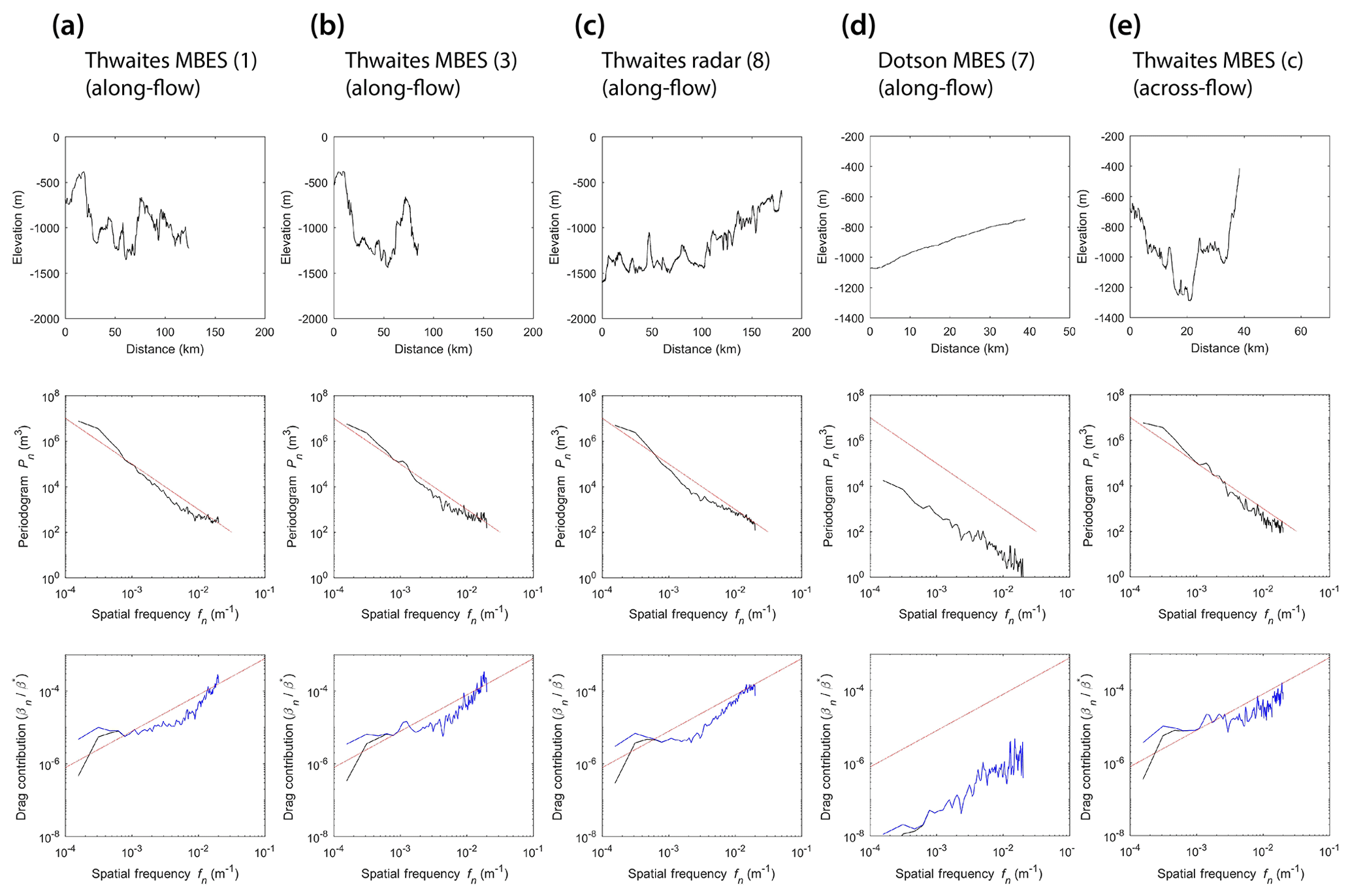
Figure 7Selection of bed profiles (top), derived power spectra (middle) and basal drag contributions (bottom) for (a, b) along-flow profiles (1) and (3) offshore Thwaites Glacier, (c) onshore along-flow bed profile (8) for Thwaites Glacier, (d) along-flow profile (7) for Dotson–Getz Trough, and (e) across-flow profile “c” offshore Thwaites Glacier. Profile locations are shown in Figs. S5 and S6. The red line in power spectra and drag contribution plots are based on an assumption of Brownian motion (i.e. power decays as inverse square of spatial frequency). At low spatial frequency, drag contributions depend on the function F. Two limiting cases are shown: F1 (blue) and F2 (black).
For Brown noise, the parameter A represents the roughness variance per unit length of profile. If we consider a section of profile having length l and restrict our definition of roughness to all wavelengths λ<l, we expect this roughness to have variance obtained by integrating the periodogram P over frequencies . For the Brown-noise periodogram (Eq. 1), this integration provides
Thus, for Brown noise, the variance grows in proportion to the section length considered, and the rms roughness grows with the square root of the section length (e.g. Jordan et al. 2017). If we take a longer section of profile, we expect to see larger rms roughness within it. This makes it clear that, at least for Brown noise, the roughness can only be characterised by its rms value if reference is also made to the length scale under consideration. Next, we examine the consequences of roughness for the drag that resists the sliding of a glacier. We pay particular attention to the case when the periodogram follows an inverse-square law (Eq. 1) that is appropriate for a Brown-noise power spectrum.
4.2 Relating bed topography to basal drag
In this section, we will use the power spectra of the high-resolution bathymetry, together with a theoretical expression for form drag (Schoof, 2002, Eq. 67), to assess how roughness at different scales affects the drag that opposes glacier sliding. This allows us to consider the contribution that the observed sea-floor bathymetric roughness at short wavelengths would make to form drag when covered by flowing ice.
The theory of ice flow over an undulating bed (Schoof, 2002) provides an approximate expression for the form drag τ, expressed as a basal shear stress that acts to resist sliding. Here, we use dimensional quantities rather than the non-dimensional quantities (as used by Schoof, 2002). In our notation, Schoof's (2002, Eq. 67) expression for form drag becomes
In this expression, β is the drag coefficient and U is the speed of ice flow averaged over some horizontal length scale significantly larger than the ice thickness. Here, we choose this length as a=6.4 km, the window length used in our spectral analysis. According to Schoof (2002), the drag coefficient is the sum of contributions, βn. Each contribution βn is caused by roughness that falls within a frequency band of width centred at frequency, . The spatial wavenumbers corresponding to these frequencies are defined as kn=2πfn.
Schoof (2002) provides an expression for the drag contributed by roughness within each frequency band. In our notation, this translates to
In this expression, is the Fourier component of the bed roughness at spatial frequency, fn. We estimate as appropriate for the Fourier series defined by Schoof (2002). The one-sided periodogram Pn can be obtained either directly from the bathymetric observations as described above (Sect. 4.1) or by fitting the inverse-square power law described by Eq. (1) to those periodograms (see Figs. 6 and 7 for examples). The scaling constants are and , where viscosity η and thickness H are representative values averaged over the length scale a (Schoof, 2002).
We consider two limiting cases for the function F:
These are derived by Schoof (2002) as his Eqs. (65) and (66) for small and large bed roughness, respectively. We use dimensional quantities, so and in our notation equate respectively to non-dimensional quantities kn, and f(kn) in Schoof (2002). For sufficiently small wavelengths , the functions and both tend to unity. In this case, the contribution to form drag becomes insensitive to ice thickness and to the choice of function used (Schoof, 2002).
If the bed follows a Brown-noise power spectrum, we can use the inverse-square law . Under those circumstances, the drag contribution βn will grow approximately linearly with frequency at sufficiently high wavenumbers :
For the Brown-noise power spectrum, the amplitude of roughness decreases at shorter wavelengths. Nevertheless, Eq. (7) shows that those short-wavelength scales will still be more effective at causing form drag than the longer wavelengths, despite their smaller amplitude. This is because the factor increases faster than the inverse-square law decreases.
As a consequence of the linear increase in the drag contribution with frequency, the total drag would become unbounded, and the sliding would stop, unless the bed of the glacier departs from the Brown-noise assumption and becomes smooth at scales smaller than some wavelength (Nye, 1970). This wavelength, λN, provides an upper bound to the spatial frequencies that cause drag, . Under this assumption, the total drag can be approximated by truncating the sum:
When λN≪a, so that N≫1, this gives the approximation
Therefore, if the Brown-noise inverse-square law power spectra applies down to the finest wavelength, λN, the drag will be determined by that scale, along with the viscosity η, and the coefficient of the power law A that can be recovered from the periodogram.
It is common in sliding theories to define the slip length, . The slip length L is an important quantity that allows us to make a distinction between two regimes of ice flow. When the slip length is much larger than the ice thickness H, the drag is too small to induce significant shearing within the ice column, and the ice can be considered to slide over the base as a plug flow having uniform velocity with depth. This is the situation modelled for slippery-based ice streams by MacAyeal (1989). By contrast, when the slip length is much smaller than the ice thickness, the drag is able to induce a substantial amount of shearing through the ice column, so the flow velocity varies significantly with depth.
Using Eq. (9), we obtain the following expression for the slip length under the assumption of a Brown-noise power spectrum, truncated at some frequency, :
One consequence of this is that if we wish to infer the amount of form drag using Eq. (9), or the slip length using Eq. (10), it is not enough to evaluate the roughness parameter A alone. We must also establish λN, the smallest wavelength that is effective at causing drag.
5.1 Bed roughnesses
The power spectra of selected bathymetric profiles are shown in Figs. 6 and 7. Figure 6b shows that the one-sided periodogram P(fn), computed using the bathymetric profile shown in Fig. 6a (location in Fig. S5a), has no strong peaks at any particular preferred scales of roughness. Instead, the periodogram decreases continuously as spatial frequency increases. This decrease approximately follows the inverse-square power law appropriate for Brown noise, so that the periodogram can be approximated as . The red line in Fig. 6b shows this power law, with a value A=0.1 m. The spectra are remarkably consistent across many of the profiles considered (Figs. 7, S7), with the exception of the smoother MSGL area (Figs. 7d, S5b). There, the Brown-noise inverse-square law can still provide a good approximation to the periodogram, but the value of A=0.001 m that is required to provide a good match to the observations is much smaller (Figs. 7, S7p, q).
The power-law approximation to the power spectrum also agrees closely with power spectra of profiles of bed elevation from airborne radar flown over TG (Fig. 7c), so the MBES data provide a good analogue to the subglacial undulations that control the sliding of TG today. Despite improvements in the methodology of high-resolution radar surveys of the active subglacial bed (King et al., 2016; Bingham et al., 2017), the MBES data provide a more detailed view of the shorter spatial scales than airborne or ground-based radar. Comparisons with previous studies of subglacial roughness are not straightforward because individual studies have used different window lengths to investigate roughness (e.g. Jordan et al., 2017; Falcini et al., 2018). However, for the Brown-noise power spectra in Eq. (1), we expect the rms roughness for a section of length l to be . Most of our spectra are close to the Brown-noise spectra with A =0.1 m (Figs. 6, 7), and for this value, we would expect window lengths from 80 to 1000 m to produce rms roughness estimates in the range 2.8 to 10 m. These values are similar to those reported previously for glaciated terrains (Jordan et al., 2017; Falcini et al., 2018).
5.2 Basal drag contributions
For the example bed profile in Fig. 6a, values of obtained using the periodogram shown in Fig. 6b and Eq. (4) are plotted against spatial frequency fn in Fig. 6c. The linear dependence predicted by Eq. (7) for the Brown-noise approximation is shown as a red line in Fig. 6c. In these plots we used a value A=0.1 m and a representative ice thickness H=1 km.
The expression for the basal slip length (Eq. 10) lets us use the bathymetry to make a dynamical distinction between regions of fast sliding with little internal deformation L>H and regions of slow sliding and shearing flow L<H. Using Eq. (10), the ratio of slip length to ice thickness is . For a value of A=0.1 m and a typical ice thickness scale of H=1 km, this suggests that features on scales smaller than λN=150 m would provide sufficient drag to induce significant vertical shearing within the ice. Since features on this scale are well resolved by the bathymetric profiles (e.g. Figs. 3, 4) and fall within the range of frequencies where the inverse-square power law applies, we conclude that the form drag produced by the observed subglacial roughness would have produced significant shearing within the flow of the grounded ice as it retreated over the highs and ridges surveyed by the MBES. This suggests that it is important to include the effects of form drag caused by basal roughness over such terrain, and by extension over the extant parts of TG today.
A distinction must be made for the region of MSGLs on the Dotson–Getz palaeo-ice-stream bed (Fig. S5b). Here, the elevation profile is exceptionally smooth. The spectral analysis confirms this (Figs. 7d, S7p, q), and the coefficient A that best fits the observations is some 2 orders of magnitude below the more generally applicable value of A=0.1 m. Repeating the above analysis with A=0.001 m shows that the power law would have to apply down to horizontal scales smaller than λN=15 m. Features on this scale are not well resolved in our bed profiles (e.g. the MBES grids have cell sizes of 50 m). This means that, in contrast to the more general case, it remains possible that the MSGL terrain is so smooth that the resulting form drag produced little vertical shearing within ice that flowed over it, making the ice dynamics of this area more akin to the flow described for slippery-based ice streams by MacAyeal (1989). This result is consistent with our understanding of how MSGLs form, i.e. via the self-organisation of deforming sediment at the bed under fast-flowing ice (e.g. Spagnolo et al., 2014). We also repeated the analysis in the direction perpendicular to elongated features (Figs. 7d, S7k–o, q). There is no evidence that ice flowed in this direction, but the theory can nevertheless compute the contributions to form drag that would arise in that hypothetical situation. For most of the across-flow lines (Fig. S7), the power spectra are similar to the along-flow direction, and the drag contributions at each frequency are similar. This suggests that the drag coefficient over much of the surveyed terrain is not especially sensitive to the flow direction. For the MSGL terrain there does appear to be some indication that drag would be higher for ice flow in the direction perpendicular to elongated features.
6.1 Implications from the new bathymetric data
Our results provide the first observation-based, high-resolution geomorphic characterisation of the coastal bathymetry at TG, a former bed for the glacier. These data allow us to investigate bathymetric controls on ocean circulation towards the modern grounding zone, as well as to identify the locations, water depths and substrate compositions of ice-shelf pinning points and former grounding zones. The dominant bathymetric features, a NNE–SSW-trending trough and landward-flanking discontinuous ridge (Fig. 2a), represent a subtly different morphologic terrain from highly rugged, basin-dominated areas north and east of the EIS (Fig. 3a) or the moderate-relief areas of lineated terrain with fewer bathymetric highs in eastern Pine Island Bay (Fig. 2a) (Nitsche et al., 2013; Arndt et al., 2018; Kirkham et al., 2019). The continuity and orientation of the trough and ridge relate to the structure of basement rocks on the inner shelf. NNE–SSW to ENE–WSW structural lineaments have been identified by previous aeromagnetic surveys (Gohl, 2012; Gohl et al., 2013), and gravity-derived bathymetries all resolve a broad NNE–SSW ridge coincident with H1–H3, as well as deeper troughs on either side of the ridge (Tinto and Bell, 2011; Millan et al., 2017; Jordan et al., 2020). Thermochronological analyses of onshore rock samples also infer a NNE–SSW-trending tectonic rift structure (Spiegel et al., 2016).
We highlight several key differences between our new dataset and the available regional bathymetric compilations (Fig. 8). Note that we do not compare our MBES grid with the newly published gravity inversion of Jordan et al. (2020) as that study utilised the MBES dataset to constrain the inversion. Beyond that study, for the area of new MBES data in front of TG, gravity-derived bathymetry generally underestimates sea-floor depths (average of 119 m; Fig. 8a, b), whereas the IBCSO bathymetry, which is based on real sea-floor soundings but relies on gravity-inversion elevations and interpolation in this area (Arndt et al., 2013), generally overestimates sea-floor depths (average of 65 m; Fig. 8c). All of the regional datasets we examined fail to capture the higher-frequency topographic variability revealed by the new MBES data (e.g. Fig. 8d). Although sea-floor highs are sometimes >100 m shallower than the regional products predict, this effect is most notable for the troughs, which are in reality 100 to 550 m deeper than gravity-derived bathymetries and 50 to 250 m deeper than in the IBCSO dataset (Fig. 8d). When we consider cross sections of three troughs that are potential pathways for CDW to the grounding zone (T2, T3, T4; locations marked by asterisks in Fig. 8a), the depth errors are up to 250, 500 and 400 m from west to east. Using a conservative top-CDW depth of 500 m for the TG area (based on hydrographic data acquired during NBP19-02; Bastien Queste, personal communication, 2020; see Nakayama et al., 2013), we calculate the cross-sectional area that CDW occupies in these troughs from our MBES data and from the grid of Millan et al. (2017). We find that the gravity-derived bathymetry underestimates the cross-sectional areas by 7 %–38 % for two of the three troughs and that trough T3 between H1 and H2 (Fig. 3a) is not resolved at all on the Millan et al. (2017) grid (Table S1; Fig. S8). Taking this one step further, we perform a simple calculation of the oceanic heat flux through T2 for the two cross-sectional areas (Millan et al., 2017; MBES) and utilise oceanographic observations from the ASE for ocean temperatures and flow velocities (see Supplement for methods). The total heat flux through the trough cross section defined by the gravity inversion is ∼0.5 TW, and for the MBES cross section it is 1.1–1.3 TW (Table S2). This equates to an underestimation of the heat flux through T2 based on the gravity-derived bathymetry of 55 %–65 %, or more than a doubling in the heat flux through the trough using the deeper bathymetry provided by the MBES grid. To fully quantify the significance of this for the inflow of CDW to the Thwaites ice-shelf cavity and grounding zone requires the use of an ocean circulation model with the MBES as its bathymetry and that is, ideally, calibrated by CTD data within the troughs. Conversely, the identification (and implementation in models) of critical sill depths along the trough pathways could limit CDW inflow along certain routes. These findings have implications for the numerical modelling of warm-water access to the grounding zone, oceanic heat fluxes, the resultant ice-shelf melting rates, and, ultimately, projected mass losses from TG and the WAIS. However, our first-pass calculations underline the importance of high-resolution observational datasets like MBES for capturing high-amplitude bathymetric variations at short to medium wavelengths (i.e. λ<103 m), particularly in areas close to ice-shelf cavities and the grounding zone.
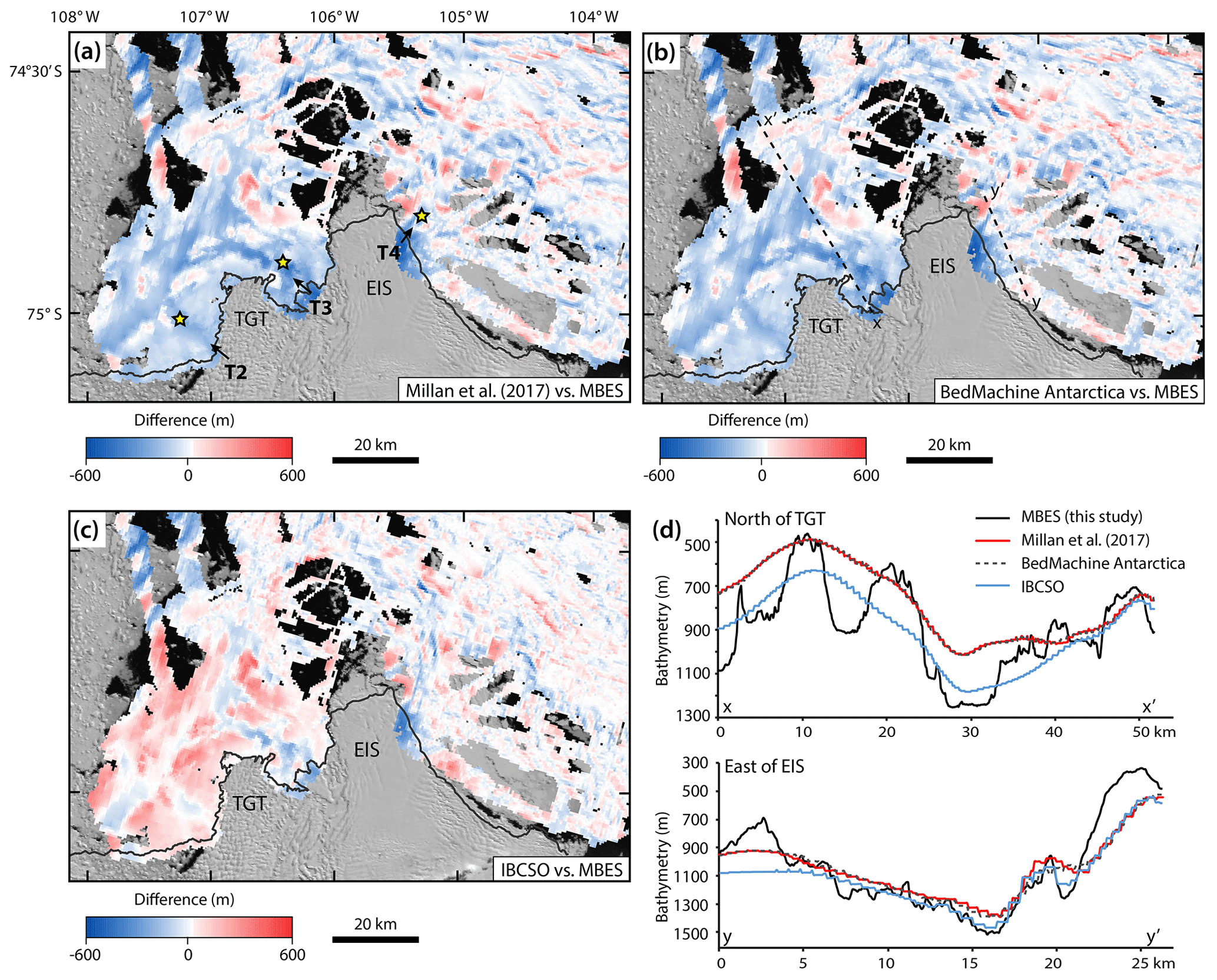
Figure 8Difference maps between regional bathymetric datasets and the MBES grid. (a) Millan et al. (2017) minus MBES grid. Yellow asterisks mark the locations of channels discussed in Sect. 6.1. (b) BedMachine Antarctica (Morlighem et al., 2019) minus MBES grid. (c) IBCSO (Arndt et al., 2013) minus MBES grid. (d) Profile data for two profiles for each of the regional datasets compared with profiles from the MBES grid; profiles are located in (b). Note that the Millan et al. (2017) and the BedMachine Antarctica bathymetries are very similar and thus return near-identical bed profiles in (d); the BedMachine Antarctica grid is included for completeness as the most recent regional dataset to cover the area, and its authors highlight the need for more coastal bathymetric datasets (Morlighem et al., 2019).
A new gravity-derived bathymetry model for the Thwaites, Crosson and Dotson–Getz area, constrained by the NBP19-02 MBES data, produced recently by Jordan et al. (2020) has improved resolution compared to previous gravity-derived models as a result of using a strapdown instrument with closer flight line spacing. Despite the improved resolution of their new model, Jordan et al. (2020) concluded that still higher-resolution observations are necessary in areas where knowledge of the bed at scales of less than a few kilometres is required. The need for high-resolution bathymetry has been underscored by recent predictive modelling studies of Antarctic outlet glaciers, which conclude that the shape of the ice-shelf cavity and knowledge of small, kilometre-scale pinning points are both key to improving predictions of ice-sheet retreat and sea-level change (Berger et al., 2016; Favier et al., 2016). Similarly, the latest high-resolution ocean models demonstrate that warm deep water reaches the grounding zone of TG through topographically constrained pathways, again highlighting the critical need for high-resolution bathymetry in making accurate predictions (Nakayama et al., 2019).
6.2 Implications from sea-floor morphology
The geometry and detailed morphology of the H1–H3 ridge also provide insight on ice-shelf pinning points. Historical grounding-zone positions, as mapped from remotely sensed ice-shelf tidal response, confirm that the Thwaites Ice Shelf is still pinned on high H1 and was pinned on high H2 as recently as 1992 and 2011 (Rignot et al., 2011). By 2011, the area of grounding on H2 had reduced to <0.5 km2 (Fig. 3a), but the recent configuration and persistence of the TGT suggests that at least some parts of it remain in (ephemeral) contact with the sea floor. Thus, the exposed H1 and H2 sea-floor highs, and by analogy H3, can be studied as current or recent pinning points for the Thwaites Ice Shelf. Glacial lineations and (or) grounding-zone wedges (GZWs) on the surface of H2 and H3, as well as rare iceberg plough marks (Fig. 4b), confirm that these pinning points are mantled by some amount of unconsolidated sediment that can be ploughed or moulded by ice. Sub-bottom profiles over the H2 and H3 highs support this as they show either an incredibly smooth sea-floor response, strongly indicative of unconsolidated sediment cover, or up to 10–15 m of unconsolidated sedimentary units (Fig. S4); furthermore, coring of the top of H3 recovered several metres of sediment (Larter et al., 2020). Although the upper section of the sediment on H3 is glacimarine, deposited after grounded ice had retreated or lifted-off from the high, the presence of a GZW there and on H2 (Fig. 4b, d) suggests that at least the uppermost part of this high may have been constructed via sedimentation at the grounding zone (see Alley et al., 1989, 2007). The potential effects of this grounding-zone sedimentation are twofold: when the TG grounding zone had retreated onto these highs during the Holocene (i.e. sometime before 10.3 ka cal BP; Hillenbrand et al., 2013), GZW formation could have temporarily slowed further retreat (Alley et al., 2007). Second, continued pinning of an ice shelf on the high and GZW, when most of the grounding line had eventually retreated further landward, would have buttressed the grounded upstream section of TG. The new MBES dataset we present here and the sea-floor landforms it reveals, supported by core recovery and sub-bottom profiles, indicate that more sediment is present in this area than is typical of other Amundsen Sea inner shelf environments that experienced rapid ice-sheet retreat, including the adjacent Pine Island Bay and the Dotson–Getz palaeo-ice-stream trough (e.g. Larter et al., 2007, 2009; Graham et al., 2009; Nitsche et al., 2013, 2016). This is likely because the grounding zone was positioned for a relatively long period of time in this area immediately offshore TG and probably because areas so close to the grounding zones of most other large glacier systems have not yet become accessible for shipborne survey. Furthermore, TG has a much larger drainage basin than the Dotson–Getz palaeo-ice-stream trough and therefore the potential to erode and deliver a greater flux of basal sediment to its grounding zone. Our only constraints on grounding-zone retreat through this area (during the Holocene) are from the core on the H1 high, which shows grounded ice withdrawal from the northern part of that high by 10.3 ka cal BP (Hillenbrand et al., 2013) and grounding zones mapped from satellite-era datasets (Rignot et al., 2011). Thus, the TG grounding zone was most probably located between H1 and the current grounding zone, potentially on the sea-floor ridges identified here, for thousands of years delivering a significant volume of sediment to the area. This retreat history is in line with what we know about deglaciation more generally in the Amundsen Sea, where rapid grounding-zone retreat occurred from 15 to 10 ka to reach near modern limits (Hillenbrand et al., 2013; Larter et al., 2014; Smith et al., 2014); however, more marine dates and terrestrial thinning histories will certainly provide additional clarity and chronological constraints for TG.
The submarine landforms observed on and around the sea-floor highs raise the question of the composition of these features. Landforms on the flanks of the pinning points (gullies, slide scars, isolated blocks; Fig. 4) may indicate that these highs consist, at least in part, of an erodible (soft) material with a probable (hard) bedrock core. In marine settings, slide scars and gullies incise large, pronounced sedimentary scarps like the shelf edge (e.g. Noormets et al., 2009; Gales et al., 2013) or the headwalls of major submarine slides (e.g. Laberg and Vorren, 2000; Vanneste et al., 2006) but do not characterise hard bedrock (crystalline) settings. Further evidence comes from the new observation of flat-topped (compacted or planed-off) morphology of the H2 and H3 highs confirming that the upper part of these (down to the level of flattening) consists of a lithology that is apparently erodible by the motion of an ice shelf (based on the orientation of lineations on the highs). Other examples of flat glacial erosion surfaces planed off by ice shelves or flat-based tabular icebergs from the Arctic all document erosion into sedimentary substrates (e.g. Vogt et al., 1994; Jakobsson et al., 2010; Noormets et al., 2016). Small (<100 m high, <5 km wide), flat-topped mounds in the Ross Sea are also thought to consist of unconsolidated volcanogenic deposits rather than crystalline bedrock, and, interestingly, GZWs have built up on them, indicating that these features slowed grounding-zone retreat in that area (Lawver et al., 2012; Greenwood et al., 2018). Although we suggest flattening of the highs by the action of Thwaites Ice Shelf, we cannot say, from our data, how much erosion may have occurred. It may be that surface sediments were simply skimmed from the tops of the highs and transported towards their seaward flanks, which, in conjunction with instabilities relating to ice-shelf grounding (or ungrounding) on the highs, could have promoted slope failures on the fronts and sides of these features (cf. Bellwald et al., 2019). Despite this caveat, all of the landform evidence presented here, supported by cores and acoustic sub-bottom profiles, suggests that the tops, fronts and sides of the H2 and H3 highs are mantled by some thickness of sediment, probably over a bedrock core. Seismic-reflection profiles would be needed to determine the internal structure of these features and sediment thicknesses. In contrast, the morphology of H1 is consistent with it having a crystalline composition. This very shallow, rugged feature is cross-cut by bedrock grooves and channels typical of hard rock exposures on the inner Antarctic shelf (Lowe and Anderson, 2002; Livingstone et al., 2013), and, although bathymetric coverage over this high is incomplete, it has few planed-off sections and no glacial lineations have been identified on its surface yet (Figs. 3b; S4b). Therefore, it is clear that there is a spatial variability in pinning point morphology and composition at TG, as well as across the wider Amundsen Sea area (Figs. 2, 5). More broadly, we also note the relative scarcity of bedrock channels or other landforms related to subglacial meltwater flow in the TG MBES dataset, with the crescentic scours (H3 only; Fig. 4a) being the exception. As an example, Kirkham et al. (2019) mapped more than 1000 subglacial channels in Pine Island Bay, whereas we map only 175 forms here, albeit over a smaller area. It is not clear whether evidence of previous meltwater routing is buried by sediment in the deep troughs or has been destroyed by ice flow over the highs. Physical-property and geochemical analyses on cores from the area, acquired as part of ITGC, should shed light on the frequency and magnitude of meltwater release during the retreat of grounded ice over the sea-floor highs. Schroeder et al. (2013) identified a transition from a distributed channel network with ponded water behind ridges at the modern grounding zone to a system of concentrated channels downstream. It is possible that a similar configuration for the basal hydrological system occurred in this area as ice retreated over the offshore highs and that evidence is preserved in the marine sedimentary record.
The apparent shaping and fragmentation of the H2 and H3 highs (Fig. 4a, b) highlights a potential feedback mechanism between bed properties (composition and topography) and glacier retreat dynamics. If the substrate of a pinning point is soft enough to be moulded by the flow of an ice shelf and to be susceptible to slope failures, it might be eroded over time. Erosion of material from the surface of a pinning point, as it is planed off, in conjunction with retrogressive failures at its seaward flank and possibly larger slide or slump events may act to reduce its surface height, as well as its surface area, by “eating away” at the frontal/side flanks until it cannot serve as a pinning point for the ice shelf (and glacier ice upstream) any longer. As long as the ice shelf continues to move over the high, this process of unpinning would be exacerbated by any increase in flow velocities (leading to increased erosion) and/or by ice-shelf thinning (leading to ungrounding), due to either flow acceleration or sub-ice-shelf melting. The result, in a setting with soft erodible pinning points, is the potential for increased ice-flow velocities to accelerate pinning point destruction which, in conjunction with simultaneous ice-shelf thinning in response to sub-ice-shelf melting, could promote ungrounding earlier than would occur on a corresponding hard, less erodible pinning point. Needless to say, in order for this feedback to occur, an ice shelf would have to continue to flow quickly over the sea-floor high(s) and not form an ice rise, under which erosion rates are considered to be low (e.g. Matsuoka et al., 2015). At TG we note that, at least for the duration of the observational record (∼55 years), the fast-flowing part of the glacier, which feeds the TGT (Fig. 2), has continued to move over the H2 and H3 highs, periodically extending several tens of kilometres before calving (Ferrigno et al., 1993; Rabus et al., 2003; MacGregor et al., 2012), whereas the ice rumple at the end of the EIS restricts flow over H1, with most ice flow being diverted around the rumple (Rignot et al., 2001). It is perhaps interesting to also consider that upwards of 50 m of relative sea-level fall due to glacio-isostatic uplift is thought to have occurred on the inner Amundsen Sea shelf during the Holocene (Whitehouse et al., 2012) and that the uplift of any pinning points would naturally counter ungrounding. Therefore, although we can only speculate on the exact mechanisms affecting rates of unpinning, we suggest that the composition of sea-floor pinning points may be an important factor in their ongoing ability to buttress large Antarctic ice shelves.
6.3 Implications from the new bed roughness data
One major objective of our research is to assess the deglaciated submarine terrain offshore from TG as an analogue for the modern bed to gain new insights on TG bed characteristics. The consistency of derived power spectra and drag contributions for bed profiles from the inner ASE shelf and for upstream areas of Pine Island and Thwaites glaciers (Figs. 7, S7) indicates that the roughness properties of the offshore and onshore areas are comparable across all resolvable frequencies. Furthermore, observations confirm that recent grounding-zone retreat affecting TG has occurred over a series of bedrock ridges with the loss of pinning points and formation of new cavities (Tinto and Bell, 2011; Milillo et al., 2019; Jordan et al., 2020). Further upstream, about 100 km from the recent grounding zone, analyses of radar specularity suggest that the modern TG bed is characterised by high roughness attributed to bedrock cropping out at the glacier base (Schroeder et al., 2014). Our data reveal that the bedrock ridges and intervening troughs underlying the modern grounding zone (Holt et al., 2006; Morlighem et al., 2019), with length scales of up to tens of kilometres and amplitudes of up to several hundreds of metres, constitute a morphological terrain similar to the coastal bathymetry (Figs. 2, 3). Further, we demonstrate that this rugged terrain would exert the same strong influence on basal drag for an overriding ice mass (assuming no cavitation) (Figs. 7, S7). This is consistent with results from inverse methods that determine basal drag for the modern TG bed (Joughin et al., 2009; Arthern et al., 2015). We also note that crag-and-tail landforms (which form subglacially) extend down to the floors of the deep troughs (e.g. Figs. 3, 4b). This confirms that, at least at the time when these features formed, ice of an expanded TG was grounded in the troughs as well as on the highs and probably experienced high basal shear similar to ice at the present-day grounding zone. The orientation of the crag and tails also confirms that ice flow was not directed along troughs but rather overrode the existing topography; this finding is consistent with cosmogenic exposure data from Bear Peninsula (Fig. 1) showing that the ice-sheet surface rose above the top of this terrain during the last glacial period (Johnson et al., 2017).
For shorter wavelengths of bed topography, we can consider the form of the individual sea-floor highs over length scales of several kilometres. We interpret the morphological characteristics of these features as being consistent with the correlation of morphology with bed type known from onshore glacial–geological studies of crag-and-tail type features (e.g. Benn and Evans, 2010), which more recently has been described from on-ice seismic-reflection profiles both for TG (Muto et al., 2019a, b; Holschuh et al., 2020) and beneath the Rutford Ice Stream (Fig. 4 in King et al., 2016). Still, we recognise that high-resolution seismic-reflection data over our bathymetric highs would be required to confirm this. Specifically, the correlation is between hard beds on the stoss sides of topographic highs, associated with crag-and-tail landforms, and soft or sedimentary beds on the lee sides of these features. This pattern is clearly replicated over the H2 and H3 highs, which have rugged upstream ends with crag-and-tail landforms, glacial lineations over their tops and sedimentary tails on their downstream ends (Fig. 4). The correlation of bed types with sea-floor highs (and ridges) holds true for several other areas of the inner shelf around West Antarctica, where streamlining of bedrock highs has often produced landforms with sedimentary tails on the lee sides of bedrock obstacles (e.g. Larter et al., 2009, Graham et al., 2009; Livingstone et al., 2013; Nitsche et al., 2013, 2016), although this is not always the case. Thus, the variability in bed types on topographic highs in offshore regions may provide useful constraints on bed type variability beneath the modern glacier.
Regarding the spectral analysis of roughness and basal drag contributions presented here (Figs. 6, 7, S7), we acknowledge that these only provide an order of magnitude assessment of the contribution to basal drag from the different wavelength scales resolved by the bathymetric DEM (Fig. 2). Analysis beyond the simple 2D-flow-line theory used here (see Sect. 4.2) would be needed to account for 3D-flow effects, as well as for the non-linear dependence of ice viscosity on stress (Glen, 1955). Here, we have not specified the physical mechanism controlling λN, the shortest roughness wavelength that influences basal drag. Candidate mechanisms that might limit the influence of roughness at small spatial scales include cavitation (Fowler, 1986), fracture and plucking of crystalline or sedimentary rocks, the formation of a weak internal shear zone (Liu et al., 2020), bulldozing of unconsolidated sediment, or regelation flow around small obstacles (Weertman, 1957). More sophisticated theories accounting for the potential of ice to form cavities in the lee of obstacles could be deployed similarly, but the drag contribution would then depend also on water pressure (Fowler, 1986; Schoof, 2005). Process models of subglacial hydrology, phase change, fracture and sediment transport could all be incorporated in to a more elaborate analysis using MBES datasets as input.
It is clear from our results that the increased spatial resolution of the MBES data is critical for capturing the high-frequency bathymetric variability on the inner continental shelf seaward of TG, which is necessary to understand warm-water incursions into sub-ice-shelf cavities (Figs. 8, S8; Nakayama et al., 2019). The strong correlation of our observations with interpretations of the present bed conditions of TG and, therefore, the robustness of this deglaciated terrain as an analogue for the modern bed further demonstrates that more information can be gleaned from this type of marine dataset (i.e. near-continuous bathymetry with spatial resolution better than 0.05 km). For example, the 3D nature of MBES (with approximately equal resolution in all directions) means that bathymetric variability could be examined in any direction, not only along survey lines, as has been the case until recently with all onshore radar or seismic-reflection profiles of extant bed topography, and over a variety of spatial scales. These analyses add to our understanding of across-flow contributions to basal drag or hydraulic potential (e.g. Muto et al., 2019a) and allow us to consider the spatial variability of bed types (e.g. sedimentary vs. hard beds), particularly where sea-floor sediments are also imaged by seismic profiles and/or cored for ground truthing. Similarly, the application of theories of subglacial processes as discussed above to high-resolution bathymetric datasets will increase our understanding of ice flow over high-frequency bed roughness, particularly if combined with ultra-high-resolution (sub-metre-resolution) bathymetries from AUV surveys (e.g. Davies et al., 2017; Dowdeswell et al., 2020). Indeed, AUV surveys and (or) a dense grid of seismic soundings (only obtainable from non-crevassed ice shelves) are the only way to determine bed geometry in ice-shelf cavities. New techniques such as swath radar that can image the present glacier bed in 3D (Paden et al., 2010; Jezek et al., 2011), albeit in narrow swaths, have already been employed on TG (Holschuh et al., 2020) and could be used in conjunction with offshore bathymetric data to build a better-informed, more complete and more uniform resolution picture of basal conditions under TG and at its grounding zone.
New 3D bathymetric data from just offshore Thwaites Glacier reveal that the coastal bathymetry is dominated by a ∼65 km long, ∼1200 m deep trough and a discontinuous ridge with water depths of 650 to <100 m. Spatial variations in the morphology of the ridge segments/highs and available acoustic sub-bottom profiler data suggest differences in substrate composition along the ridge, with the two southernmost highs having a significant erodible component at least in their upper parts, which are sedimentary in composition. The geometry (flat tops) and landform evidence (glacial lineations, gullies, sediment fans) indicate that the bathymetric highs were planed off and variously eroded by the action of Thwaites Ice Shelf as it flowed over them, presumably reducing the height of these former pinning points over time. A feedback mechanism during unpinning may have occurred, whereby as the ice shelf started to lose contact with the high and frontal buttressing weakened, the resultant increase in flow velocities exacerbated erosion of the high and facilitated further unpinning of Thwaites Glacier.
We present three lines of evidence that this coastal bathymetry provides a good analogue for the modern grounding zone of Thwaites Glacier. First, on length scales of several tens of kilometres, the ridge and trough morphology is consistent with the bed topography of the grounding-zone area based on available DEMs and over-ice geophysical data. Second, our spectral decomposition of roughness and basal drag over this rugged, deglaciated terrain is consistent with similar spectral decompositions, and inversions of basal drag, for profiles from the modern grounding zone area and for areas of the Thwaites bed, where bedrock crops out subglacially (e.g. Schroeder et al., 2014). In contrast, smooth beds, characterised by thick sedimentary substrates and linear glacial landforms, produce distinctly different power spectra and drag contributions. Third, the distribution of landforms and substrate types (unconsolidated sediment vs. bedrock) over the ridge indicates that it displays the same correlation of bed type with topography that has been described for upstream bed areas and inferred for the grounding zone (Muto et al., 2019a, b; Holschuh et al., 2020). As such, further analyses of this deglaciated terrain may provide realistic constraints on across-flow roughness and bed type distribution and should inform geophysical observations of the modern TG bed that will be acquired as part of ITGC.
As discussed above, observational datasets like MBES are required seaward of Antarctic ice shelves in order to capture the high-frequency variability that characterises the bathymetry of nearshore areas. Bathymetry derived from gravity inversions cannot adequately reproduce the kilometre- to sub-kilometre-scale features that are important for accurately calculating inflows of warm ocean water in troughs and for defining the topographic highs that may act as pinning points for ice shelves and as barriers to warm-water incursions.
Processed MBES data grids with grid spacings of 50 and 500 m are available from the UK Polar Data Centre https://doi.org/10.5285/F2DFEDA9-BF44-4EF5-89A3-EE5E434A385C (Hogan et al., 2020). Raw data sources are indicated in Table 1.
The supplement related to this article is available online at: https://doi.org/10.5194/tc-14-2883-2020-supplement.
KAH, RDL, RA, TAJ and AGCG developed the concept of the paper. KAH, RDL, AGCG, RLT, JDK, RC and VF acquired and performed initial processing on the bathymetry data during NBP19-02; JDK performed all channel metric analyses. KG, JEA and JH provided bathymetric data from German and Korean cruises, respectively. KAH compiled, part-processed, and gridded all bathymetric datasets and wrote the first draft of the paper with substantial contributions from RA and RDL. RA developed the methodology, performed spectral analyses and basal drag estimations, and wrote the text for these sections; KAH and TAJ provided the profile data. AW performed the ocean heat flux calculations. All authors contributed to the development of the final paper and data visualisation.
The authors declare that they have no conflict of interest.
This work is an output of the Thwaites Offshore Research (THOR) project and Glacial Habitat of Subglacial Thwaites (GHOST) projects, components of the International Thwaites Glacier Collaboration (ITGC). Logistics were provided by the NSF United States Antarctic Program and the NERC British Antarctic Survey. ITGC contribution no. ITGC-011. We thank the NBP19-02 science party, the Edison Chouset Offshore Inc. captain and crew, and the Antarctic Support Contract technical staff aboard the RV/IB Nathaniel B. Palmer. In addition to the editor and reviewers, we are also grateful to Nick Holschuh for constructive comments on the submitted manuscript. This study is part of the Polar Science for Planet Earth programme of the British Antarctic Survey.
This research has been supported by the National Science Foundation, Office of Polar Programs (grant no. 1738942), the Natural Environment Research Council (grant nos. NE/S006664/1 and NE/S006672/1).
This paper was edited by Chris R. Stokes and reviewed by Martin Jakobsson and Matteo Spagnolo.
Alley, R. B., Anandakrishnan, S., Dupont, T. K., Parizek, B. R., and Pollard, D.: Effect of sedimentation on ice-sheet grounding-line stability, Science, 315, 1838–1841, 2007.
Alley, R. B., Blankenship, D. D., Rooney, S. T., and Bentley, C. R.: Sedimentation beneath ice shelves – the view from ice stream B, Mar. Geol., 85, 101–120, 1989.
Arndt, J. E., Larter, R. D., Friedl, P., Gohl, K., Höppner, K., and the Science Team of Expedition PS104: Bathymetric controls on calving processes at Pine Island Glacier, The Cryosphere, 12, 2039–2050, https://doi.org/10.5194/tc-12-2039-2018, 2018.
Arndt, J. E., Schenke, H. W., Jakobsson, M., Nitsche, F. O., Buys, G., Goleby, B., Rebesco, M., Bohoyo, F., Hong, J., Black, J., Greku, R., Udintsev, G., Barrios, F., Reynoso-Peralta, W., Taisei, M., and Wigley, R.: The International Bathymetric Chart of the Southern Ocean (IBCSO) Version 1.0 – A new bathymetric compilation covering circum-Antarctic waters, Geophys. Res. Lett., 40, 3111–3117, https://doi.org/10.1002/grl.50413, 2013.
Arthern, R. J., Hindmarsh, R. C. A., and Williams, C. R.: Flow speed within the Antarctic ice sheet and its controls inferred from satellite observations, J. Geophys. Res.-Earth, 120, 1171–1188, 2015.
Bellwald, B., Hjelstuen, B. O., Sejrup, H. P., Stokowy, T., and Kuvås, J.: Holocene mass movements in west and mid-Norwegian fjords and lakes, Mar. Geol., 407, 192–212, 2019.
Benn, D. I. and Evans, D. J. A.: Glaciers and Glaciation, 2nd Edn., Hodder, Education, London, 802 pp., ISBN 978-0-340-905791, 2010.
Berger, S., Favier, L., Drews, R., Derwael, J.-J., and Pattyn, F.: The control of an uncharted pinning point on the flow of an Antarctic ice shelf, J. Glaciol., 62, 37–45, 2016.
Bingham, R. G., Vaughan, D. G., King, E. C., Davies, D., Cornford, S. L., Smith, A. M., Arthern, R. J., Brisbourne, A. M., De Rydt, J., Graham, A. G. C., Spagnolo, M., Marsh, O. J., and Shean, D. E.: Diverse landscapes beneath Pine Island Glacier influence ice flow, Nat. Commun., 8, 1618, 2017.
Caress, D. W. and Chayes, D. N.: Improved processing of Hydrosweep DS multibeam data on the R/V Maurice Ewing, Mar. Geophys. Res., 18, 631–650, 1996.
Caress, D. W., Chayes, D. N., and Ferreira, C.: MB-System Seafloor Mapping Software, available at: https://www.mbari.org/products/research-software/mb-system/, last access: 12 February 2020.
Clark, C. D., Tulaczyk, S. M., Stokes, C. R., and Canals, M.: A groove-ploughing theory for the production of mega-scale glacial lineations, and implications for ice-stream mechanics, J. Glaciol., 49, 240–256, 2003.
Davies, D., Bingham, R. G., Graham, A. G. C., Spagnolo, M., Dutrieux, P., Vaughan, D. G., Jenkins, A., and Nitsche, F. O.: High-resolution sub-ice-shelf seafloor records of twentieth century ungrounding and retreat of Pine Island Glacier, West Antarctica, J. Geophys. Res.-Earth, 122, 1698–1714, 2017.
De Rydt, J. and Gudmundsson, G. H.: Coupled ice shelf-ocean modeling and complex grounding line retreat from a seabed ridge, J. Geophys. Res.-Earth, 121, 865–880, 2016.
De Rydt, J., Holland, P. R., Dutrieux, P., and Jenkins, A.: Geometric and oceanographic controls on melting beneath Pine Island Glacier, J. Geophys. Res.-Oceans, 119, 2420–2438, 2014.
Dowdeswell, J. A., Batchelor, C. L., Montelli, A., Ottesen, D., Christie, F. D. W., Dowdeswell, E. K., and Evans, J.: Delicate seafloor landforms reveal past Antarctic grounding-line retreat of kilometers per year, Science, 368, 1020, 2020.
Dowdeswell, E. K., Todd, B. J., and Dowdeswell, J. A.: Crag-and-tail features: convergent ice flow through Eclipse Sound, Baffin Island, Arctic Canada, edited by: Dowdeswell, J. A., Canals, M., Jakobsson, M., Todd, B. J., Dowdeswell, E. K., and Hogan, K. A., Geological Society, London, Memoirs, 46, 55–56, https://doi.org/10.1144/M46.106, 2016.
Dowdeswell, J. A. and Fugelli, E. M. G.: The seismic architecture and geometry of grounding-zone wedges formed at the marine margins of past ice sheets, Geol. Soc. Am. Bull., 124, 1750–1761, 2012.
Dutrieux, P., De Rydt, J., Jenkins, A., Holland, P. R., Ha, H. K., Lee, S. H., Steig, E. J., Ding, Q., Abrahamsen, E. P., and Schröder, M.: Strong Sensitivity of Pine Island Ice-Shelf Melting to Climatic Variability, Science, 343, 174–178, https://doi.org/10.1126/science.1244341, 2014.
Evans, J., Dowdeswell, J. A., Ó Cofaigh, C., Benham, T. J., and Anderson, J. B.: Extent and dynamics of the West Antarctic Ice Sheet on the outer continental shelf of Pine Island Bay during the last glaciation, Mar. Geol., 230, 53–72, 2006.
Falcini, F. M., Rippin, D. M., Krabbendam, M., and Selby, K. A.: Quantifying bed roughness beneath contemporary and palaeo-ice streams, J. Glaciol., 64, 822–834, 2018.
Favier, L., Durand, G., Cornford, S. L., Gudmundsson, G. H., Gagliardini, O., Gillet-Chaulet, F., Zwinger, T., Payne, A. J., and Le Brocq, A. M.: Retreat of Pine Island Glacier controlled by marine ice-sheet instability, Nat. Clim. Change, 4, 117–121, 2014.
Favier, L., Pattyn, F., Berger, S., and Drews, R.: Dynamic influence of pinning points on marine ice-sheet stability: a numerical study in Dronning Maud Land, East Antarctica, The Cryosphere, 10, 2623–2635, https://doi.org/10.5194/tc-10-2623-2016, 2016.
Ferrigno, J. G., Lucchitta, B. K., Mullins, K. F., Allison, A. L., Allen, R. J., and Gould, W. G.: Velocity measurements and changes in position of Thwaites Glacier/iceberg tongue from aerial photography, Landsat images and NOAA AVHRR data, Ann. Glaciol., 17, 239–244, 1993.
Fowler, A. C. and Nye, J. F.: A sliding law for glaciers of constant viscosity in the presence of subglacial cavitation, P. R. Soc.-Math. Phys. Sc., 407, 147–170, 1986.
Gales, J. A., Larter, R. D., Mitchell, N. C., and Dowdeswell, J. A.: Geomorphic signature of Antarctic submarine gullies: Implications for continental slope processes, Mar. Geol., 337, 112–124, 2013.
Glen, J. W. and Perutz, M. F.: The creep of polycrystalline ice, P. R. Soc.-Math. Phys. Sc., 228, 519–538, 1955.
Gohl, K.: Basement control on past ice sheet dynamics in the Amundsen Sea Embayment, West Antarctica, Palaeogeogr. Palaeocl., 335–336, 35–41, 2012.
Gohl, K., Denk, A., Eagles, G., and Wobbe, F.: Deciphering tectonic phases of the Amundsen Sea Embayment shelf, West Antarctica, from a magnetic anomaly grid, Tectonophysics, 585, 113–123, 2013.
Graham, A. G. C. and Hogan, K. A.: Crescentic scours on palaeo-ice stream beds, edited by: Dowdeswell, J. A., Canals, M., Jakobsson, M., Todd, B. J., Dowdeswell, E. K., and Hogan, K. A., Memoirs, Geological Society, London, 46, 221–222, https://doi.org/10.1144/M46.166, 2016.
Graham, A. G. C., Larter, R. D., Gohl, K., Hillenbrand, C.-D., Smith, J. A., and Kuhn, G.: Bedform signature of a West Antarctic palaeo-ice stream reveals a multi-temporal record of flow and substrate control, Quaternary Sci. Rev., 28, 2774–2793, 2009.
Graham, A. G. C., Larter, R. D., Gohl, K., Dowdeswell, J. A., Hillenbrand, C.-D., Smith, J. A., Evans, J., Kuhn, G., and Deen, T.: Flow and retreat of the Late Quaternary Pine Island‐Thwaites palaeo‐ice stream, West Antarctica, J. Geophys. Res., 115, F03025, https://doi.org/10.1029/2009JF001482, 2010.
Greenwood, S. L., Simkins, L. M., Halberstadt, A. R. W., Prothro, L. O., and Anderson, J. B.: Holocene reconfiguration and readvance of the East Antarctic Ice Sheet, Nat. Commun., 9, 3176, 2018.
Ha, H. K., Wåhlin, A. K., Kim, T. W., Lee, S. H., Lee, J. H., Lee, H. J., Hong, C. S., Arneborg, L., Björk, G., and Kalén, O.: Circulation and Modification of Warm Deep Water on the Central Amundsen Shelf, J. Phys. Oceanogr., 44, 1493–1501, 2014.
Heywood, K. J., Biddle, L. C., Boehme, L., Dutrieux, P., Fedak, M., Jenkins, A., Jones, R. W., Kaiser, J., Mallett, H., Garabato, A. C. N., Renfrew, I. A., Stevens, D. P., and Webber, B. G. M.: Between the Devil and the Deep Blue Sea: The Role of the Amundsen Sea Continental Shelf in Exchanges Between Ocean and Ice Shelves, Oceanography, 29, 118–129, 2016.
Hillenbrand, C.-D., Kuhn, G., Smith, J. A., Gohl, K., Graham, A. G. C., Larter, R. D., Klages, J. P., Downey, R., Moreton, S. G., Forwick, M., and Vaughan, D. G.: Grounding-line retreat of the West Antarctic Ice Sheet from inner Pine Island Bay, Geology, 41, 35–38, 2013.
Hogan, K. A., Dowdeswell, J. A., and Mienert, J.: New insights into slide processes and seafloor geology revealed by side-scan imagery of the massive Hinlopen Slide, Arctic Ocean margin, Geo-Mar. Lett., 33, 325–343, 2013.
Hogan, K. A., Larter, R. D., Graham, A. G. C., Nitsche, F. O., Kirkham, J. D., Totten Minzoni, R., Clark, R., Fitzgerald, V., Anderson, J. B., Hillenbrand, C.-D., Simkins, L., Smith, J. A., Gohl, K., Arndt, J. E., Hong, J., Heywood, K. J., Abrahamsen, E. P., Thompson, A. F., Dunbar, R., and Wellner, J. S.: A multibeam-bathymetric compilation for the southern Amundsen Sea shelf, 1999–2019 (Version 1.0) [Data set], UK Polar Data Centre, Natural Environment Research Council, UK Research & Innovation, https://doi.org/10.5285/F2DFEDA9-BF44-4EF5-89A3-EE5E434A385C, 2020.
Holschuh, N., Christianson, K., Paden, J., Alley, R. B., and Anandakrishnan, S.: Linking postglacial landscapes to glacier dynamics using swath radar imaging at Thwaites Glacier, Antarctica, Geology, 48, 268–272, 2020.
Holt, J. W., Blankenship, D. D., Morse, D. L., Young, D. A., Peters, M. E., Kempf, S. D., Richter, T. G., Vaughan, D. G., and Corr, H. F. J.: New boundary conditions for the West Antarctic Ice Sheet: Subglacial topography of the Thwaites and Smith glacier catchments, Geophys. Res. Lett., 33, L09502, https://doi.org/10.1029/2005GL025561, 2006.
Hubbard, B., Siegert, M. J., and McCarroll, D.: Spectral roughness of glaciated bedrock geomorphic surfaces: Implications for glacier sliding, J. Geophys. Res.-Sol. Ea., 105, 21295–21303, 2000.
Hughes, T. J.: The weak underbelly of the West Antarctic ice sheet, J. Glaciol., 27, 518–525, 1981.
Jacobs, S., Giulivi, C., Dutrieux, P., Rignot, E., Nitsche, F., and Mouginot, J.: Getz Ice Shelf melting response to changes in ocean forcing, J. Geophys. Res.-Oceans, 118, 4152–4168, 2013.
Jacobs, S., Jenkins, A., Hellmer, H., Giulivi, C., Nitsche, F., Huber, B., and Guerrero, R.: The Amundsen Sea and the Antarctic Ice Sheet, Oceanography, 25, 154–163, 2012.
Jacobs, S. S., Hellmer, H. H., and Jenkins, A.: Antarctic Ice Sheet melting in the southeast Pacific, Geophys. Res. Lett., 23, 957–960, 1996.
Jakobsson, M., Anderson, J. B., Nitsche, F. O., Gyllencreutz, R., Kirshner, A. E., Kirchner, N., O'Regan, M., Mohammad, R., and Eriksson, B.: Ice sheet retreat dynamics inferred from glacial morphology of the central Pine Island Bay Trough, West Antarctica, Quaternary Sci. Rev., 38, 1–10, 2012.
Jakobsson, M., Nilsson, J., O'Regan, M., Backman, J., Löwemark, L., Dowdeswell, J. A., Mayer, L., Polyak, L., Colleoni, F., Anderson, L., Björk, G., Darby, D., Eriksson, B., Hanslik, D., Hell, B., Marcussen, C., Sellén, E., and Wallin, Å.: An Arctic Ocean ice shelf during MIS 6 constrained by new geophysical and geological data, Quaternary Sci. Rev., 29, 3505–3517, 2010.
Jenkins, A., Dutrieux, P., Jacobs, S. S., McPhail, S. D., Perrett, J. R., Webb, A. T., and White, D.: Observations beneath Pine Island Glacier in West Antarctica and implications for its retreat, Nat. Geosci., 3, 468–472, 2010.
Jenkins, A., Dutrieux, P., Jacobs, S., Steig, E. J., Gudmundsson, G. H., Smith, J., and Heywood, K. J.: Decadal Ocean Forcing and Antarctic Ice Sheet Response: Lessons from the Amundsen Sea, Oceanography, 29, 106–117, 2016.
Jezek, K., Wu, X., Gogineni, P., Rodríguez, E., Freeman, A., Rodriguez-Morales, F., and Clark, C. D.: Radar images of the bed of the Greenland Ice Sheet, Geophys. Res. Lett., 38, 1–5, https://doi.org/10.1029/2010GL045519, 2011.
Johnson, J. S., Smith, J. A., Schaefer, J. M., Young, N. E., Goehring, B. M., Hillenbrand, C.-D., Lamp, J. L., Finkel, R. C., and Gohl, K.: The last glaciation of Bear Peninsula, central Amundsen Sea Embayment of Antarctica: Constraints on timing and duration revealed by in situ cosmogenic 14C and 10Be dating, Quaternary Sci. Rev., 178, 77–88, 2017.
Jordan, T. A., Porter, D., Tinto, K., Millan, R., Muto, A., Hogan, K., Larter, R. D., Graham, A. G. C., and Pade, J. D.: New gravity-derived bathymetry for the Thwaites, Crosson, and Dotson ice shelves revealing two ice shelf populations, The Cryosphere, 14, 2869–2882, https://doi.org/10.5194/tc-14-2869-2020, 2020.
Jordan, T. M., Cooper, M. A., Schroeder, D. M., Williams, C. N., Paden, J. D., Siegert, M. J., and Bamber, J. L.: Self-affine subglacial roughness: consequences for radar scattering and basal water discrimination in northern Greenland, The Cryosphere, 11, 1247–1264, https://doi.org/10.5194/tc-11-1247-2017, 2017.
Joughin, I., Tulaczyk, S., Bamber, J. L., Blankenship, D., Holt, J. W., Scambos, T., and Vaughan, D. G.: Basal conditions for Pine Island and Thwaites Glaciers, West Antarctica, determined using satellite and airborne data, J. Glaciol., 55, 245–257, 2009.
Joughin, I., Smith, B. E., and Holland, D. M.: Sensitivity of 21st century sea level to ocean-induced thinning of Pine Island Glacier, Antarctica, Geophys. Res. Lett., 37, L20502, https://doi.org/10.1029/2010GL044819, 2010.
Joughin, I., Smith, B. E., and Medley, B.: Marine Ice Sheet Collapse Potentially Under Way for the Thwaites Glacier Basin, West Antarctica, Science, 344, 735, 2014.
Kamb, B.: Sliding motion of glaciers: theory and observation, Reviews of Geophysics and Space Physics, 8, 673–728, 1970.
Kim, J.-W., Kim, D.-j., Kim, S. H., Ha, H. K., and Lee, S. H.: Disintegration and acceleration of Thwaites Ice Shelf on the Amundsen Sea revealed from remote sensing measurements, Gisci. Remote Sens., 52, 498–509, 2015.
King, E. C., Pritchard, H. D., and Smith, A. M.: Subglacial landforms beneath Rutford Ice Stream, Antarctica: detailed bed topography from ice-penetrating radar, Earth Syst. Sci. Data, 8, 151–158, 2016.
Kirkham, J. D., Hogan, K. A., Larter, R. D., Arnold, N. S., Nitsche, F. O., Golledge, N. R., and Dowdeswell, J. A.: Past water flow beneath Pine Island and Thwaites glaciers, West Antarctica, The Cryosphere, 13, 1959–1981, https://doi.org/10.5194/tc-13-1959-2019, 2019.
Kirshner, A., Anderson, J.B., Jakobsson, M., O'Regan, M., Majewski, W., and Nitsche, F.: Post-LGM deglaciation in Pine island Bay, west Antarctica. Quaternary Sci. Rev., 38, 11–26, 2012.
Kuhn, G., Hillenbrand, C.-D., Kasten, S., Smith, J. A., Nitsche, F. O., Frederichs, T., Wiers, S., Ehrmann, W., Klages, J. P., and Mogollón, J. M.: Evidence for a palaeo-subglacial lake on the Antarctic continental shelf, Nat. Commun., 8, 15591, https://doi.org/10.1038/ncomms15591, 2017.
Larter, R. D., Gohl, K., Hillenbrand, C.-D., Kuhn, G., Deen, T. J., Dietrich, R., Eagles, G., Johnson, J. S., Livermore, R. A., Nitsche, F. O., Pudsey, C. J., Schenke, H.-W., Smith, J. A., Udintsev, G., and Uenzelmann-Neben, G.: West Antarctic Ice Sheet change since the Last Glacial Period, Eos T. Am. Geophys. Un., 88, 189–190, 2007.
Larter, R. D., Graham, A. G. C., Gohl, K., Kuhn, G., Hillenbrand, C.-D., Smith, J. A., Deen, T. J., Livermore, R. A., and Schenke, H.-W.: Subglacial bedforms reveal complex basal regime in a zone of paleo–ice stream convergence, Amundsen Sea embayment, West Antarctica, Geology, 37, 411–414, 2009.
Larter, R. D., Anderson, J. B., Graham, A. G. C., Gohl, K., Hillenbrand, C-. D., Jakobsson, M., Johnson, J. S., Kuhn, G., Nitsche, F. O., Smith, J. A., Witus, A. E., Bentley, M. J., Dowdeswell, J. A., Ehrmann, W., Klages, J. P., Lindow, J., O Cofaigh, C., and Spiegel, C.: Reconstruction of changes in the Amundsen Sea ad Bellingshausen Sea sector of the West Antarctic Ice Sheet since the Last Glacial Maximum, Quaternary Sci. Rev., 100, 55–86, 2014.
Larter, R. D., Queste, B. Y., Boehme, L., Braddock, S., Wåhlin, A. K., Graham, A. G. C., Hogan, K. A., Totten Minzoni, R., Barham, M., Bortolotto de'Oliveira, G., Clark, R., Fitzgerald, V., Karam, S., Kirkham, J. D., Mazur, A., Sheehan, P., Spoth, M., Stedt, P., Welzenbach, L. Zheng, Y., Andersson, J., Rolandsson, J., Beeler, C., Goodell, J., Rush, and Snow, T.: CRUISE REPORT RV/IB Nathaniel B. Palmer Cruise NBP19-02, January-March 2019: First research cruise of the International Thwaites Glacier Collaboration, http://get.rvdata.us/cruise/NBP1902/doc/NBP1902_report_final.pdf (last access: 11 June 2020), 2020.
Larter, R. D. and Vanneste, L. E.: Relict subglacial deltas on the Antarctic Peninsula outer shelf, Geology, 23, 33–36, 1995.
Livingstone, S. J., Cofaigh, C. Ó., Stokes, C. R., Hillenbrand, C.-D., Vieli, A., and Jamieson, S. S. R.: Glacial geomorphology of Marguerite Bay Palaeo-Ice stream, western Antarctic Peninsula, J. Maps, 9, 558–572, 2013.
Liu, E. W., Räss, L., Suckale, J., Herman, F., and Podladchikov, Y.: Spontaneous Formation of Internal Shear Zone in Ice Flowing over a Topographically Variable Bed, EGU General Assembly 2020, Online, 4–8 May 2020, EGU2020-12602, https://doi.org/10.5194/egusphere-egu2020-12602, 2020.
Lowe, A. L. and Anderson, J. B.: Evidence for abundant subglacial meltwater beneath the paleo-ice sheet in Pine Island Bay, Antarctica, J. Glaciol., 49, 125–138, 2003.
Lowe, A. L. and Anderson, J. B.: Reconstruction of the West Antarctic ice sheet in Pine Island Bay during the Last Glacial Maximum and its subsequent retreat history, Quaternary Sci. Rev., 21, 1879–1897, 2002.
MacAyeal, D. R.: Large-scale ice flow over a viscous basal sediment: Theory and application to ice stream B, Antarctica, J. Geophys. Res.-Sol. Ea., 94, 4071–4087, 1989.
MacGregor, J. A., Catania, G. A., Markowski, M. S., and Andrews, A. G.: Widespread rifting and retreat of ice-shelf margins in the eastern Amundsen Sea Embayment between 1972 and 2011, J. Glaciol., 58, 458–466, 2012.
MacLean, B., Blasco, S., Bennett, R., Hughes Clarke, J. E., and Patton, E.: Crag-and-tail features, Amundsen Gulf, Canadian Arctic Archipelago, edited by: Dowdeswell, J. A., Canals, M., Jakobsson, M., Todd, B. J., Dowdeswell, E. K., and Hogan, K. A., Memoirs, Geological Society, London, 46, 53–54, https://doi.org/10.1144/M46.84, 2016.
Matsuoka, K., Hindmarsh, R. C. A., Moholdt, G., Bentley, M. J., Pritchard, H. D., Brown, J., Conway, H., Drews, R., Durand., G., Goldberg, D., Hattermann, T., Kingslake, J., Lenaerts, J. T. M., Martín, C., Mulvaney, R., Nicholss, K. W., Pattyn, F., Ross, N., Scambos, T., and Whitehouse, P. L.: Antarctic ice rises and rumples: Their properties and significance for ice-sheet dynamics and evolution, Earth Sci. Rev., 150, 724–745, 2015.
Mayer, L. A., Paton, M., Gee, L., Gardner, S. V., and Ware, C.: Interactive 3-D visualization: a tool for seafloor navigation, exploration and engineering, in: Proceedings of the OCEANS 2000 MTS/IEEE Conference and Exhibition, Providence, USA, 11–14 September 200, 913–919, 2000.
McMillan, M., Shepherd, A., Sundal, A., Briggs, K., Muir, A., Ridout, A., Hogg, A., and Wingham, D.: Increased ice losses from Antarctica detected by CryoSat-2, Geophys. Res. Lett., 41, 3899–3905, 2014.
Milillo, P., Rignot, E., Rizzoli, P., Scheuchl, B., Mouginot, J., Bueso-Bello, J., and Prats-Iraola, P.: Heterogeneous retreat and ice melt of Thwaites Glacier, West Antarctica, Science Advances, 5, eaau3433, https://doi.org/10.1126/sciadv.aau3433, 2019.
Millan, R., Rignot, E., Bernier, V., Morlighem, M., and Dutrieux, P.: Bathymetry of the Amundsen Sea Embayment sector of West Antarctica from Operation IceBridge gravity and other data, Geophys. Res. Lett., 44, 1360–1368, 2017.
Morlighem, M., Rignot, E., Binder, T., Blankenship, D., Drews, R., Eagles, G., Eisen, O., Ferraccioli, F., Forsberg, R., Fretwell, P., Goel, V., Greenbaum, J. S., Gudmundsson, H., Guo, J., Helm, V., Hofstede, C., Howat, I., Humbert, A., Jokat, W., Karlsson, N. B., Lee, W. S., Matsuoka, K., Millan, R., Mouginot, J., Paden, J., Pattyn, F., Roberts, J., Rosier, S., Ruppel, A., Seroussi, H., Smith, E. C., Steinhage, D., Sun, B., Broeke, M. R. v. d., Ommen, T. D. v., Wessem, M. v., and Young, D. A.: Deep glacial troughs and stabilizing ridges unveiled beneath the margins of the Antarctic ice sheet, Nat. Geosci., 13, 132–137, https://doi.org/10.1038/s41561-019-0510-8, 2019.
Mouginot, J., Rignot, E., and Scheuchl, B.: Continent-Wide, Interferometric SAR Phase, Mapping of Antarctic Ice Velocity, Geophys. Res. Lett., 46, 9710–9718, 2019.
Mouginot, J., Rignot, E., and Scheuchl, B.: Sustained increase in ice discharge from the Amundsen Sea Embayment, West Antarctica, from 1973 to 2013, Geophys. Res. Lett., 41, 1576–1584, 2014.
Muto, A., Alley, R. B., Parizek, B. R., and Anandakrishnan, S.: Bed-type variability and till (dis)continuity beneath Thwaites Glacier, West Antarctica, Ann. Glaciol., 60, 82–90, https://doi.org/10.1017/aog.2019.32, 2019a.
Muto, A., Anandakrishnan, S., Alley, R. B., Horgan, H. J., Parizek, B. R., Koellner, S., Christianson, K., and Holschuh, N.: Relating bed character and subglacial morphology using seismic data from Thwaites Glacier, West Antarctica, Earth Planet Sc. Lett., 507, 199–206, 2019b.
Nakayama, Y., Manucharyan, G., Zhang, H., Dutrieux, P., Torres, H. S., Klein, P., Seroussi, H., Schodlok, M., Rignot, E., and Menemenlis, D.: Pathways of ocean heat towards Pine Island and Thwaites grounding lines, Sci. Rep., 9, 16649, https://doi.org/10.1038/s41598-019-53190-6, 2019.
Nakayama, Y., Schröder, M., and Hellmer, H. H.: From circumpolar deep water to the glacial meltwater plume on the eastern Amundsen Shelf, Deep-Sea Res. Pt. I, 77, 50–62, 2013.
Nitsche, F. O., Gohl, K., Larter, R. D., Hillenbrand, C.-D., Kuhn, G., Smith, J. A., Jacobs, S., Anderson, J. B., and Jakobsson, M.: Paleo ice flow and subglacial meltwater dynamics in Pine Island Bay, West Antarctica, The Cryosphere, 7, 249–262, https://doi.org/10.5194/tc-7-249-2013, 2013.
Nitsche, F. O., Jacobs, S. S., Larter, R. D., and Gohl, K.: Bathymetry of the Amundsen Sea continental shelf: Implications for geology, oceanography, and glaciology, Geochem. Geophy. Geosy., 8, Q10009, https://doi.org/10.1029/2007GC001694, 2007.
Nitsche, F. O., Larter, R. D., Gohl, K., Graham, A. G. C., and Kuhn, G.: Crag-and-tail features on the Amundsen Sea continental shelf, West Antarctica, edited by: Dowdeswell, J. A., Canals, M., Jakobsson, M., Todd, B. J., Dowdeswell, E. K., and Hogan, K. A., Memoirs, Geological Society, London, 46, 199–200, https://doi.org/10.1144/M46.2, 2016.
Noormets, R., Dowdeswell, J. A., Larter, R. D., Ó Cofaigh, C., and Evans, J.: Morphology of the upper continental slope in the Bellingshausen and Amundsen Seas - Implications for sedimentary processes at the shelf edge of West Antarctica, Mar. Geol., 258, 100–114, 2009.
Noormets, R., Kirchner, N., Flink, A. E., and Dowdeswell, J. A.: Possible iceberg-produced submarine terraces in Hambergbukta, Spitsbergen, edited by: Dowdeswell, J. A., Canals, M., Jakobsson, M., Todd, B. J., Dowdeswell, E. K., and Hogan, K. A., Memoirs, Geolhttps://doi.org/10.1144/M46.121, 2016.
Nye, J. F.: Glacier sliding without cavitation in a linear viscous approximation, P. Roy. Soc. A-Math. Phy., 315, 381–403, 1970.
Ó Cofaigh, C., Dowdeswell, J. A., Allen, C. S., Hiemstra, J. F., Pudsy, C., J., Evans, J., Evans, D. J. A.: Flow dynamics and till genesis associated with a marine-based Antarctic palaeo-ice stream, Quaternary Sci. Rev., 24, 709–740, 2005.
Paden, J., Akins, T., Dunson, D., Allen, C., and Gogineni, P.: Ice-sheet bed 3-D tomography, J. Glaciol., 56, 3–11, https://doi.org/10.3189/002214310791190811, 2010.
Parizek, B. R. and Walker, R. T.: Implications of initial conditions and ice–ocean coupling for grounding-line evolution, Earth Planet Sc. Lett., 300, 351–358, 2010.
Pattyn, F. and Van Huele, W.: Power law or power flaw?, Earth Surface Processes and Landforms, 23, 761–767, 1998.
Post, A. L., O'Brien, P. E., Edwards, S., Carroll, A. G., Malakoff, K., and Armand, L. K.: Upper slope processes and seafloor ecosystems on the Sabrina continental slope, East Antarctica, Mar. Geol., 422, 106091, https://doi.org/10.1016/j.margeo.2019.106091, 2020.
Rabus, B. T., Lang, O., and Adolphs, U.: Interannual velocity variations and recent calving of Thwaites Glacier Tongue, West Antarctica, Ann. Glaciol., 36, 215–224, 2003.
Rignot, E.: Evidence for rapid retreat and mass loss of Thwaites Glacier, West Antarctica, J. Glaciol., 47, 213–222, 2001.
Rignot, E., Jacobs, S., Mouginot, J., and Scheuchl, B.: Ice-Shelf Melting Around Antarctica, Science, 341, 266–270, 2013.
Rignot, E., Mouginot, J., Morlighem, M., Seroussi, H., and Scheuchl, B.: Widespread, rapid grounding line retreat of Pine Island, Thwaites, Smith, and Kohler glaciers, West Antarctica, from 1992 to 2011, Geophys. Res. Lett., 41, 3502–3509, 2014.
Rignot, E., Mouginot, J., and Scheuchl, B.: Antarctic grounding line mapping from differential satellite radar interferometry, Geophys. Res. Lett., 38, L10504, https://doi.org/10.1029/2011GL047109, 2011.
Rignot, E., Mouginot, J., Scheuchl, B., van den Broeke, M., van Wessem, M. J., and Morlighem, M.: Four decades of Antarctic Ice Sheet mass balance from 1979–2017, P. Natl. Acad. Sci. USA, 116, 1095, 2019.
Rippin, D. M., Vaughan, D. G., and Corr, H. F. J.: The basal roughness of Pine Island Glacier, West Antarctica, J. Glaciol., 57, 67–76, 2011.
Scambos, T. A., Bell, R. E., Alley, R. B., Anandakrishnan, S., Bromwich, D. H., Brunt, K., Christianson, K., Creyts, T., Das, S. B., DeConto, R., Dutrieux, P., Fricker, H. A., Holland, D., MacGregor, J., Medley, B., Nicolas, J. P., Pollard, D., Siegfried, M. R., Smith, A. M., Steig, E. J., Trusel, L. D., Vaughan, D. G., and Yager, P. L.: How much, how fast?: A science review and outlook for research on the instability of Antarctica's Thwaites Glacier in the 21st century, Global Planet. Change, 153, 16–34, 2017.
Schoof, C.: Basal perturbations under ice streams: form drag and surface expression, J. Glaciol., 48, 407–416, 2002.
Schoof, C.: The effect of cavitation on glacier sliding, P. Roy. Soc. A-Math. Phy., 461, 609–627, 2005.
Schoof, C.: Ice sheet grounding line dynamics: Steady states, stability, and hysteresis, J. Geophys. Res.-Earth, 112, F03S28, https://doi.org/10.1029/2006JF000664, 2007.
Schroeder, D. M., Blankenship, D. D., and Young, D. A.: Evidence for a water system transition beneath Thwaites Glacier, West Antarctica, P. Natl. Acad. Sci. USA, 110, 12225, 2013.
Schroeder, D. M., Blankenship, D. D., Young, D. A., Witus, A. E., and Anderson, J. B.: Airborne radar sounding evidence for deformable sediments and outcropping bedrock beneath Thwaites Glacier, West Antarctica, Geophys. Res. Lett., 41, 7200–7208, 2014.
Shepherd, A., Gilbert, L., Muir, A. S., Konrad, H., McMillan, M., Slater, T., Briggs, K. H., Sundal, A. V., Hogg, A. E., and Engdahl, M. E.: Trends in Antarctic Ice Sheet Elevation and Mass, Geophys. Res. Lett., 46, 8174–8183, 2019.
Siegert, M. J., Taylor, J., Payne, A. J., and Hubbard, B.: Macro-scale bed roughness of the Siple Coast ice streams in west Antarctica, Earth Surface Processes and Landforms, 29, 1591–1596, 2004.
Spagnolo, M., Clark, C. D., Ely, J. C., Stokes, C. R., Anderson, J. B., Andreassen, K., Graham, A. G. C., and King, E. C.: Size, shape and spatial arrangement of mega-scale glacial lineations from a large and diverse dataset, Earth Surface Processes and Landforms, 39, 1432–1448, 2014.
Spagnolo, M., Bartholomaus, T. C., Clark, C. D., Stokes, C. R., Atkinson, N., Dowdeswell, J. A., Ely, J. C., Graham, A. G. C., Hogan, K. A., King, E. C., Larter, R. D., Livingstone, S. J., and Pritchard, H. D.: The periodic topography of ice stream beds: Insights from the Fourier spectra of mega-scale glacial lineations, J. Geophys. Res.-Earth, 122, 1355–1373, 2017.
Spiegel, C., Lindow, J., Kamp, P. J. J., Meisel, O., Mukasa, S., Lisker, F., Kuhn, G., and Gohl, K.: Tectonomorphic evolution of Marie Byrd Land – Implications for Cenozoic rifting activity and onset of West Antarctic glaciation, Global Planet. Change, 145, 98–115, 2016.
Tinto, K. J. and Bell, R. E.: Progressive unpinning of Thwaites Glacier from newly identified offshore ridge: Constraints from aerogravity, Geophys. Res. Lett., 38, L20503, https://doi.org/10.1029/2011GL049026, 2011.
Tinto, K., Bell, R. E., and Cochran, J. R.: IceBridge Sander AIRGrav L1B Geolocated Free Air Gravity Anomalies, Version 1.05, NASA National Snow and Ice Data Center Distributed Active Archive Center, Boulder, Colorado USA, https://doi.org/10.5067/R1RQ6NRIJV89, 2010 (updated 2019).
Vanneste, M., Mienert, J., and Bünz, S.: The Hinlopen Slide: A giant, submarine slope failure on the northern Svalbard margin, Arctic Ocean, Earth Planet Sc. Lett., 245, 373–388, 2006.
Vaughan, D. G. and Arthern, R.: Why Is It Hard to Predict the Future of Ice Sheets?, Science, 315, 1503, 2007.
Vaughan, D. G., Smith, A.M., Corr, H. F. J., Jenkins, A., Bentley, C. R., Stenoien, M. D., Jacobs, S. S., Kellogg, T. B., Rignot, E., and Lucchitta, B. K.: A Review of Pine Island Glacier, West Antarctica: Hypotheses of Instability vs. Observations of Change, American Geophysical Union, Washington, D.C., Antarctic Research Series, 77, 237–256, 2001.
Vogt, P. R., Crane, K., and Sundvor, E.: Deep Pleistocene iceberg plowmarks on the Yermak Plateau: sidescan and 3.5 kHz evidence for thick calving ice fronts and a possible marine ice sheet in the Arctic Ocean, Geology, 22, 403–406, 1994.
Walker, D. P., Brandon, M. A., Jenkins, A., Allen, J. T., Dowdeswell, J. A., and Evans, J.: Oceanic heat transport onto the Amundsen Sea shelf through a submarine glacial trough, Geophys. Res. Lett., 34, L02602, https://doi.org/10.1029/2006GL028154, 2007.
Weertman, J.: On the Sliding of Glaciers, J. Glaciol., 3, 33–38, 1957.
Weertman, J.: Stability of the junction between an ice sheet and an ice shelf, J. Glaciol., 13, 3–11, 1974.
Welch, P. D.: The Use of Fast Fourier Transform for the Estimation of Power Spectra: A Method Based on Time Averaging Over Short, Modified Periodograms, IEEE T. Acoust. Speech., 15, 70–73, 1967.
Wellner, J. S., Heroy, D. C., and Anderson, J. B.: The death mask of the Antarctic ice sheet: Comparison of glacial geomorphic features across the continental shelf, Geomorphology, 75, 157–171, 2006.
Whitehouse, P. L., Bentley, M. J., Milne, G. A., King, M. A. and Thomas, I. D.: A new glacial isostatic adjustment model for Antarctica: calibrated and tested using observations of relative sea-level change and present-day uplift rates, Geophys. J. Int., 190, 1464–1482, 2012.
- Abstract
- Introduction
- Methods I: multibeam echo-sounder (MBES) datasets
- Results I: a new bathymetric compilation for the inner Amundsen Sea Embayment shelf
- Methods II: bed roughness and basal drag
- Results II: assessing roughness and drag contributions for palaeo- and modern glacier beds
- Discussion
- Conclusions
- Data availability
- Author contributions
- Competing interests
- Acknowledgements
- Financial support
- Review statement
- References
- Supplement