A linear model to derive melt pond depth on Arctic sea ice from hyperspectral data

Melt ponds are key elements in the energy balance of Arctic sea ice. Observing their temporal evolution is crucial for understanding melt processes and predicting sea ice evolution. Remote sensing is the only technique that enables large-scale observations of Arctic sea ice. However, monitoring melt pond deepening in this way is challenging because most of the optical signal reflected by a pond is defined by the scattering characteristics of the underlying ice. Without knowing the influence of meltwater on the reflected signal, the water depth cannot be determined. To solve the problem, we simulated the way meltwater changes the reflected spectra of bare ice. We developed a model based on the slope of the log-scaled remote sensing reflectance at 710 nm as a function of depth that is widely independent from the bottom albedo and accounts for the influence of varying solar zenith angles. We validated the model using 49 in situ melt pond spectra and corresponding depths from shallow ponds on dark and bright ice. Retrieved pond depths are accurate (root mean square error, RMSE=2.81 cm; nRMSE=16 %) and highly correlated with in situ measurements (r=0.89; $p=\mathrm{4.34}\times {\mathrm{10}}^{-\mathrm{17}}$). The model further explains a large portion of the variation in pond depth (R²=0.74). Our results indicate that our model enables the accurate retrieval of pond depth on Arctic sea ice from optical data under clear sky conditions without having to consider pond bottom albedo. This technique is potentially transferrable to hyperspectral remote sensors on unmanned aerial vehicles, aircraft and satellites.

1 Introduction

Melt ponds on sea ice are key elements for the Arctic energy budget. They are a main driver of the ice–albedo feedback mechanism (Curry et al., 1995) and affect the mass and heat balance of sea ice (e.g., Flocco et al., 2012; Perovich et al., 2009). Observations of pond evolution can be linked to observations of sea ice, ocean and atmosphere (e.g., Inoue et al., 2008; Polashenski et al., 2012; Webster et al., 2015) for validation of ice and climate models (e.g., Flocco et al., 2012) and future sea ice prediction (e.g., Schröder et al., 2014). In the context of climate change, it is therefore important to increase our understanding of how melt ponds on sea ice change (Lee et al., 2012).

Recent efforts were made to observe the evolution of melt pond fraction with satellite data (e.g., Istomina et al., 2015a, 2015b; Rösel et al., 2012; Tschudi et al., 2008; Zege et al., 2015), but few studies investigated melt pond depth despite its relevance for many applications. Melt pond depth is a parameter in the Los Alamos sea ice model CICE (Flocco et al., 2012; Hunke et al., 2013) and the ECHAM5 general circulation model (Pedersen et al., 2009). Lecomte et al. (2011) used pond depth to parameterize melt pond albedo in a snow scheme for the thermodynamic component of the Louvain-la-Neuve sea ice model. Holland et al. (2012) related pond water volume to surface meltwater fluxes in the community climate system model, version 4, and Palmer et al. (2014) used melt pond depths to model primary production below sea ice. Liu et al. (2015) point out that climate models and forecast systems that account for realistic melt pond evolution “seem to be a worthy area of expanded research and development” (Liu et al., 2015) and question the suitability of statistical forecasting methods in the context of the changing Arctic, which points towards the need for regular observations with large spatial coverage.

Synoptic observations of melt pond evolution are only possible with satellite remote sensing. Optical sensors with an adequate spatial resolution that operate in the visible (VIS) and near-infrared (NIR) wavelength regions enable the monitoring of pond water characteristics. The reflected optical signal from melt ponds without ice cover contains information on the pond water, the pond bottom, underlying ice and skylight reflected at the water surface.

Some studies investigated the potential to map the bathymetry of melt ponds with optical data in supraglacial lakes on the Greenland ice sheet. Tedesco and Steinar (2011) used the model of Philpot (1989) for optically shallow water and resampled hyperspectral reflectance measurements from below the water surface to Landsat and MODIS bands in order to explore its capability to derive the depth of a supraglacial lake. Due to the strong absorption of water in the near infrared, they limited the data range to 450–650 nm and excluded depth measurements <1 m “because of the relatively small sensitivity of the reflectance data in the Landsat and MODIS blue and green bands to shallow waters” (Tedesco and Steiner, 2011). In comparison with shallow water sonar measurements, they underestimated depth by −23.7% and −42.7% for Landsat bands 1 and 2, respectively. Legleiter et al. (2014) used hyperspectral remote sensing reflectance measurements above the water surface to map the bathymetry of supraglacial lakes and streams. They used an optimal band ratio analysis to find suitable band combinations for calibrating an empirical model based on field measurements on the Greenland ice sheet. A model based on two bands in the yellow–orange wavelength region resulted in an R² of 0.92 and a standard error of 0.47 m for depths ranging between 0.31 and 10.45 m. While this accuracy may be sufficient for glacial lakes, the maximum depth of ponds on sea ice is restricted by its thickness and therefore seldom exceeds 1 m (e.g., Morassutti and Ledrew, 1996; Perovich et al., 2009).

The color of melt ponds on sea ice ranges from bright blue to almost black and is primarily defined by the scattering and, to a lesser degree, by the absorption characteristics of the pond bottom (Lu et al., 2016, 2017). Different radiative transfer models for melt ponds on sea ice exist, but their capability to derive pond depth varies. Lu et al. (2016, 2017) developed a two-stream radiative transfer model to retrieve pond depth and the thickness of the underlying ice from RGB images but did not find a clear relationship between simulated and measured pond depth using the data from Istomina et al. (2016). To our knowledge, the most accurate model is the one presented in Malinka et al. (2018) resulting in an R² of 0.62 (N=26) for in situ pond depths between 6 and 50 cm acquired under different illumination conditions. Their analytical two-stream radiative transfer model links the spectral albedo of ponds between 350 and 1300 nm at various sky conditions to pond depth and transport scattering coefficient and thickness of the bottom ice. Fitting these parameters during inverse computation of in situ datasets from three field campaigns accurately reproduced in situ albedo spectra (relative root mean square difference, rRMSD<1.5 %), but pond depth retrieval was more uncertain (rRMSD=65 %).

We hypothesize that instead of using the entire spectrum, selecting bands in the near-infrared wavelength region improves the retrieval of pond depth on sea ice from optical data. The penetration depth of light into water is highest in the blue region of the electromagnetic spectrum and decreases with increasing wavelength; i.e., with increasing wavelength the influence of the water column's attenuation on the optical signal increases (Pope and Fry, 1997). Mapping the bathymetry of supraglacial lakes with a two-band model is challenging because the attenuation of water is wavelength dependent and the range of depths is wide. For shallow ponds on sea ice, Morassutti and Ledrew (1996) stated that the influence of water absorption on the pond albedo increases towards the NIR wavelength region. Lu et al. (2016) found that pond albedo significantly depends on pond depth in the wavelength region between 600 and 900 nm. In this paper, we therefore present a linear pond depth model for Arctic sea ice based on the absorption of near-infrared light in water from hyperspectral optical measurements under clear sky conditions.

2 Methods

We use spectral data of bare ice surfaces to simulate melt pond spectra for model development and validate the model with in situ melt pond measurements acquired during RV Polarstern cruise PS106 in summer 2017.

2.1 Observational data

We used two instrument setups for the acquisition of optical data. For most measurements, we used a combination of two Ocean Optics STS-VIS spectrometers (Ocean Optics Inc., USA): one spectrometer pointing downwards and equipped with a 1^∘ fore optic, the other pointing upwards and equipped with a cosine collector. Both instruments cover the wavelength region from ∼340 to ∼820 nm with a spectral resolution of 3.0 nm (Ocean Optics, 2019). We used a Labsphere Spectralon^® 99 % diffuse reflectance standard (Labsphere Inc., USA) as white reference and applied the data from the second spectrometer to correct the reflectance spectra for changes in downwelling irradiance. For each measurement, we computed the average of 30 individual spectra. Both instruments were mounted on the end of a 1 m long pole to avoid influences of the polar clothes on the measurements. We also attached a camera to the setup to take photographs of each measurement site (Fig. 1).

Some of the data used in this study were acquired within the scope of an angle-resolving bidirectional reflectance distribution function (BRDF) experiment. For these measurements, we used an Ibsen Freedom VIS FSV-305 spectrometer (Ibsen Photonics A/S, Denmark) with a spectral resolution of 1.8 nm covering the wavelength range from ∼360 to ∼830 nm (Ibsen Photonics, 2019). The spectrometer was equipped with an optical fiber and a 1^∘ fore optic that were attached to a field goniometer (Fig. 2). We used the above-mentioned Spectralon^® panel as white reference after each azimuthal scan and computed an average reflectance from 20 spectra.

The quantity measured with both spectrometer setups is the remote sensing reflectance (R_rs; sr⁻¹) above the water surface:

$$\begin{array}{}\text{(1)}& {\displaystyle }{\displaystyle }{R}_{\text{rs}}={\displaystyle \frac{L_{\mathrm{u}}}{E_{\mathrm{d}}}},\end{array}$$

where L_u is upwelling radiance – W (m² nm sr)⁻¹ – measured by the downward-pointing sensor and E_d is downwelling irradiance – W (m² nm)⁻¹ – which is derived from the Spectralon^® measurement as

$$\begin{array}{}\text{(2)}& {\displaystyle }{\displaystyle }{E}_{\mathrm{d}}={\displaystyle \frac{L_{\mathrm{S}}\cdot \mathit{\pi }}{R_{\mathrm{S}}}},\end{array}$$

where R_S is the isotropic reflectance of the Spectralon^® panel and L_S is a radiance measurement – W (m² nm sr)⁻¹ – of the Spectralon^® panel.

2.1.1 Ice spectra

On 15 June 2017, we used the Ocean Optics setup to collect spectra from three bright and one dark bare ice surfaces (Gege et al., 2019) that were missing the typical surface scattering layer (Fig. 1a, b). We therefore assume that their optical properties are comparable to pond bottoms. Illumination was diffuse and stable which was indicated by the negligible standard deviation of the 30 spectra contained in one measurement (Fig. 1c).

Figure 1 Photos of bright (a) and dark (b) bare ice surfaces and respective reflectance spectra (c). We took the photos from approximately 50 cm (a) and 30 cm (b) above the surface.

On 2 July 2017 between 00:35 and 01:18 LST, we performed 12 nadir measurements of a bare ice surface, likewise missing a surface scattering layer (Fig. 2a), under clear sky conditions and a mean solar zenith angle of 74.89^∘ with the Ibsen setup (Gege and König, 2019). Here we use the average spectrum. The large standard deviation may be attributed to surface metamorphism during the measurement (Fig. 2b).

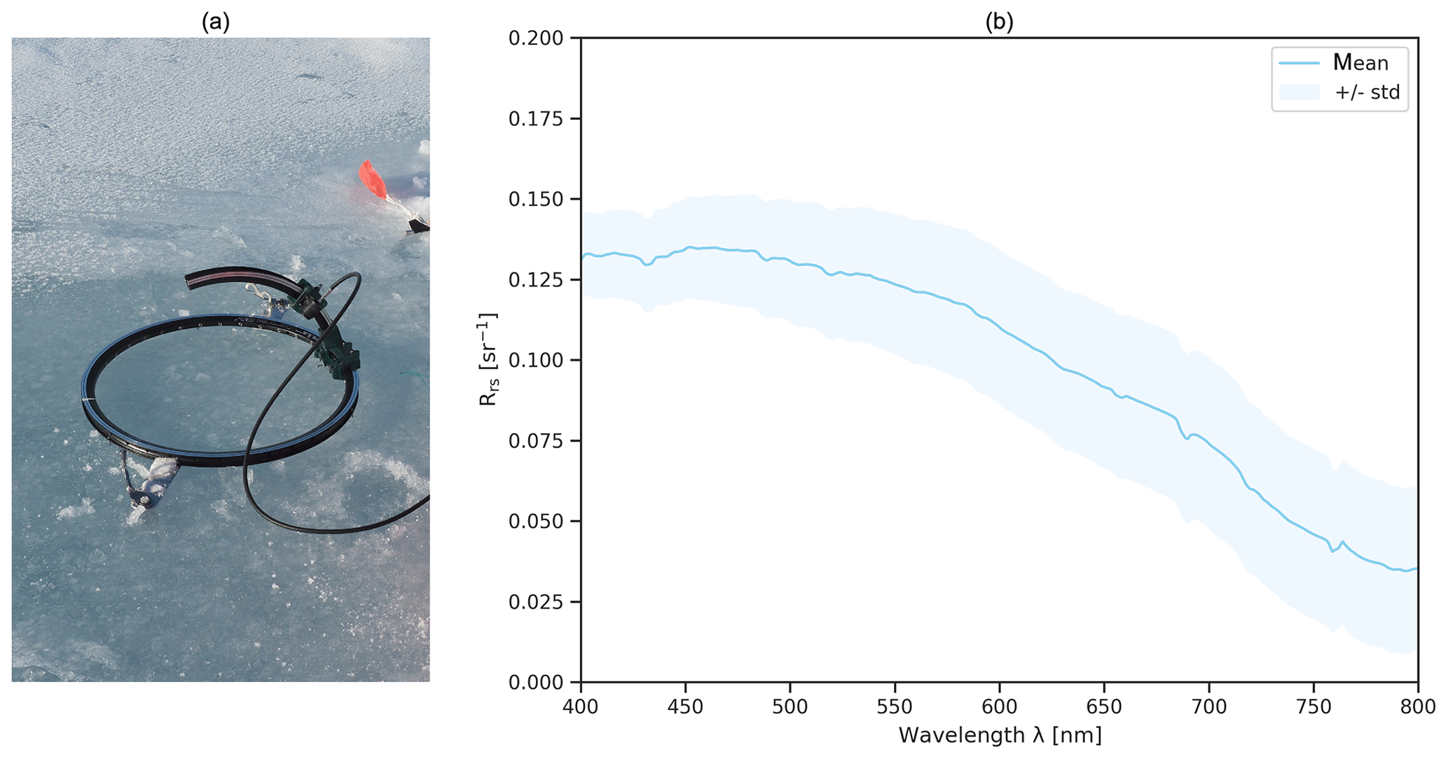
Figure 2 Ibsen bare ice measurement setup (a). Spectra used in this study (b) were taken at nadir.

2.1.2 Pond measurements

On 10 June 2017, we collected 49 melt pond spectra (Gege et al., 2019) and corresponding pond depths in three melt ponds. Two of the ponds had a bright blue color, while the third one was very dark, which is also apparent in Fig. 3. The pond site was located in a ridged area, and ice thickness measurements from 14 June 2017 showed that ice thickness was ≥0.9 m below the bright ponds and ≤0.5 m below the dark pond, which indicates that the bright ice is older. We presume that the dark ice may have been a refrozen lead. However, no ice cores were analyzed to determine the respective ice types.

Figure 3 Overview of measurement sites in the three ponds. Aerial photo: Gerit Birnbaum.

The bottoms of the bright ponds were mostly smooth and solid but also featured a few cracks and highly scattering areas that were very porous. The dark pond bottom was more heterogeneous and featured cracks and areas that were porous and riddled with holes (Fig. 4).

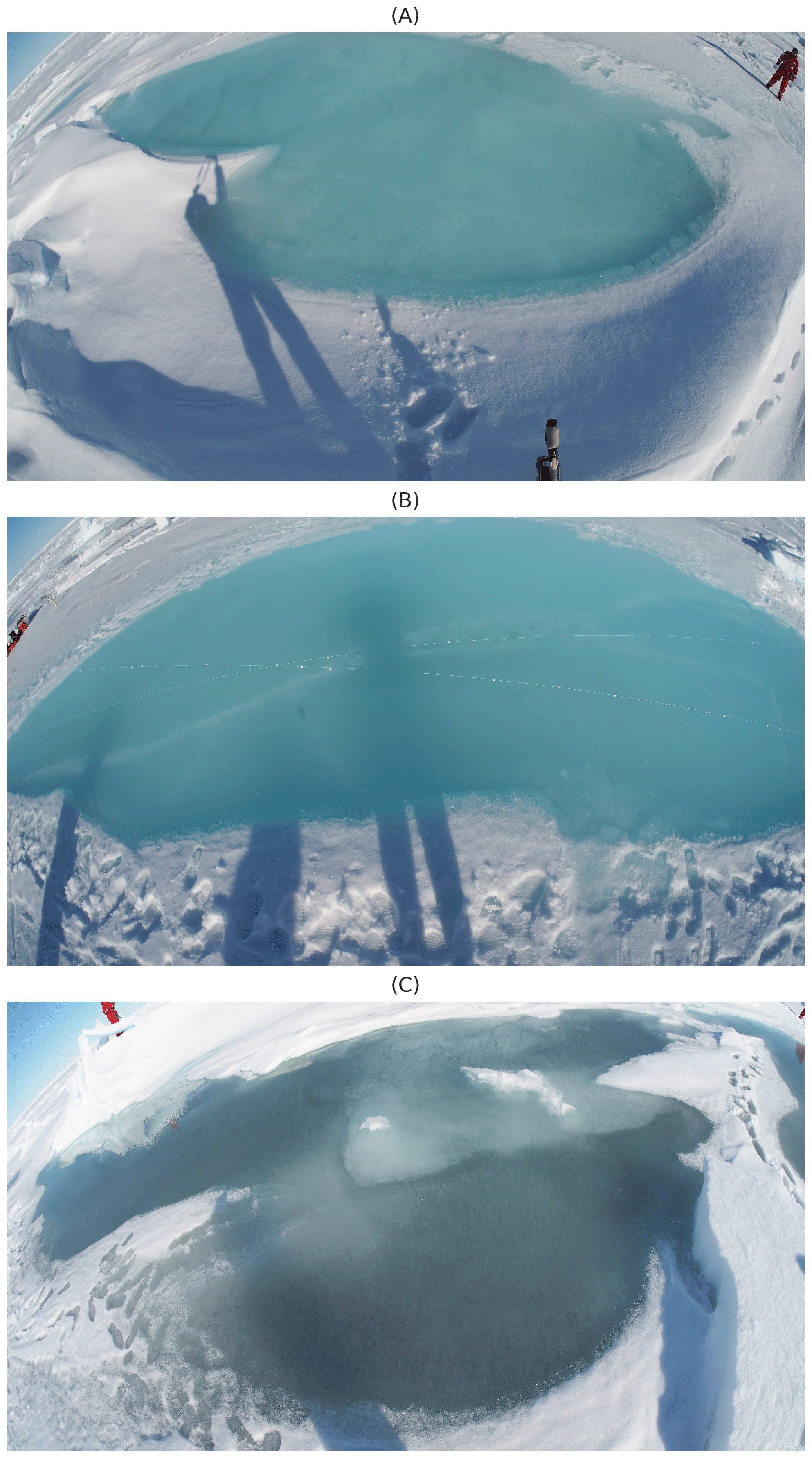
Figure 4 Photos of the small (a) and large (b) bright ponds and the dark pond (c). Photos: Peter Gege.

At each pond, we referenced the Ocean Optics spectrometers using the Spectralon^® panel before data acquisition. We performed spectral measurements from the edge of the pond or waded through the pond avoiding shading. We did not observe any wind-induced disturbances of the water surface and waited for the water surface to settle before performing measurements inside the ponds. All measurements were performed under clear sky conditions between 12:23 LST and 14:43 LST and corresponding solar zenith angles between 58.90 and 61.04^∘. Directly after each spectral measurement, we used a folding ruler to measure pond depth at the same location. Depths ranged between 6 and 25 cm with an average of 17.60 cm. Figure 5 illustrates the melt pond spectra and corresponding pond depths.

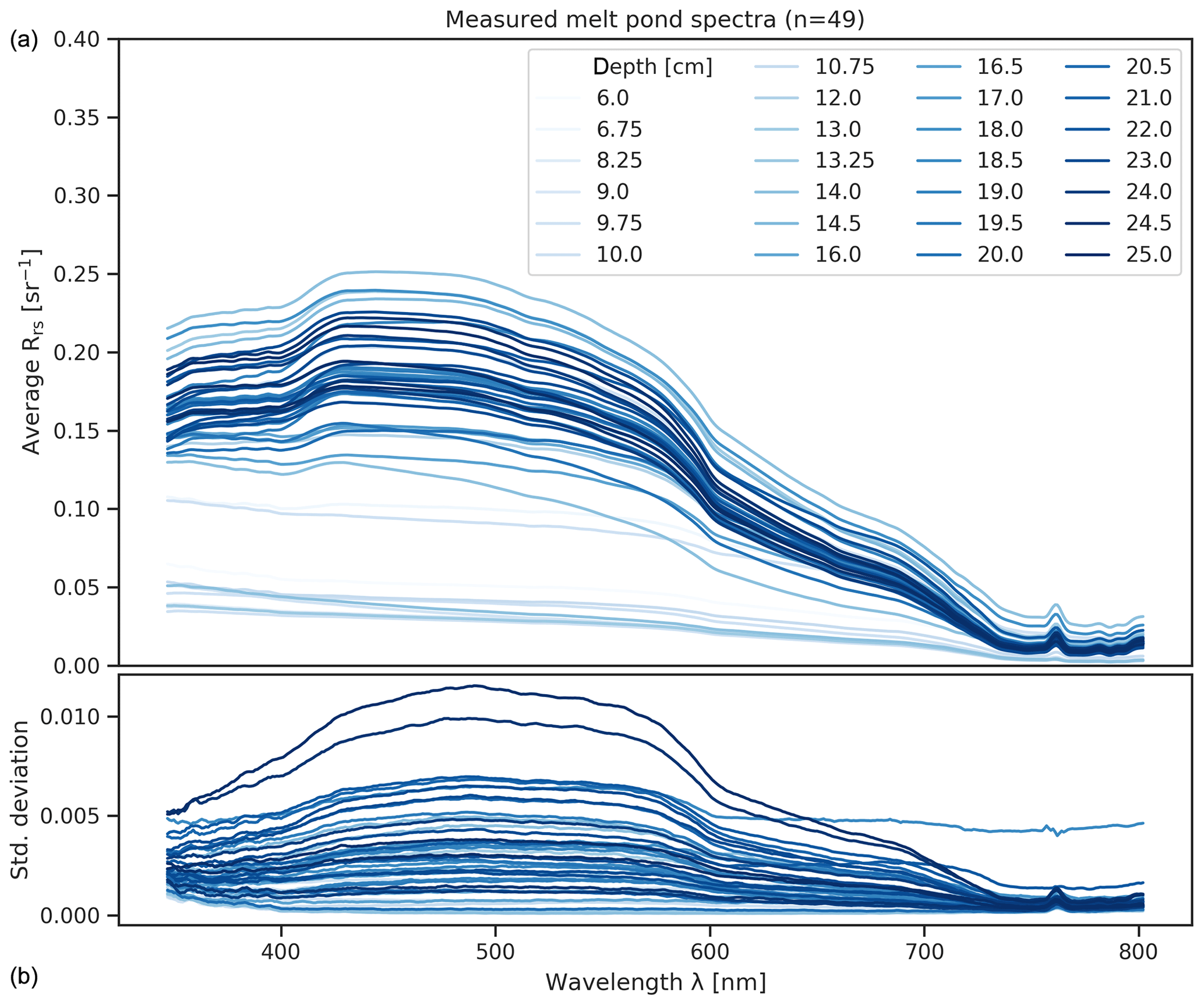
Figure 5 Average reflectance spectra (a), standard deviation of 30 measurements (b) and corresponding pond depths.

2.1.3 Data smoothing

Even though the spectra appear smooth at first view, the hardly visible amount of noise in the data becomes relevant for calculating derivatives. To smooth the spectra, we therefore resampled all spectra to a 1 nm spectral sampling by linear interpolation and then applied a running average filter with a width of 5 nm.

2.2 Model development

To develop an approach that does not require knowledge about on-site ice characteristics, our model must be independent from changes in the bottom albedo, i.e., scattering characteristics of the underlying ice. It shall further be applicable to a wide range of pond depths up to 1.0 m. Because the in situ melt pond dataset is limited to shallow depths and biased towards bright blueish ponds, we used the water color simulator (WASI) to create a spectral library covering different bottom type mixtures and depths. WASI is a software tool for the analysis and simulation of deep and shallow water spectra that is based on well-established analytical models (Gege, 2004, 2014, 2015; Gege and Albert, 2006). We used the forward mode of the program WASI-2D (v4.1) to generate libraries of melt pond spectra. The procedures are described in the following.

2.2.1 Simulated data

We used the Ocean Optics bare ice spectra from overcast sky conditions (Sect. 2.1.1) as pond bottom reflectance.

Analyses of optical properties of water samples showed only negligible amounts of chlorophyll a, colored dissolved organic matter and total suspended matter. Moreover, Podgorny and Grenfell (1996) report that the signal of scattering in meltwater is overwhelmed by the scattering in the bottom ice. We therefore defined a pure water column without additional absorbing or scattering water constituents and computed remote sensing reflectance in shallow water above the water surface according to Eq. (2.20b) in Gege (2015):

$$\begin{array}{ll}{\displaystyle }& {\displaystyle }{R}_{\text{rs}}^{\text{sh}}\left(\mathit{\lambda }\right)={\displaystyle \frac{(\mathrm{1}-\mathit{\sigma })(\mathrm{1}-{\mathit{\sigma }}_L^{-})}{n_{\mathrm{w}}^{\mathrm{2}}}}\cdot {\displaystyle \frac{R_{\text{rs}}^{\text{sh}-}\left(\mathit{\lambda }\right)}{\mathrm{1}-{\mathit{\rho }}_{\mathrm{u}}\cdot Q\cdot R_{\text{rs}}^{\text{sh}-}\left(\mathit{\lambda }\right)}}\\ \text{(3)}& {\displaystyle }& {\displaystyle }+R_{\text{rs}}^{\text{surf}}\left(\mathit{\lambda }\right),\end{array}$$

where σ, ${\mathit{\sigma }}_L^{-}$ and ρ_u are the reflection factors for E_d and upwelling radiance ($L_{\mathrm{u}}^{-}$) and irradiance just below the water surface. σ and ρ_u are 0.03 and 0.54, respectively, while ${\mathit{\sigma }}_L^{-}$ is calculated from the viewing angle (0^∘ for a nadir-directed sensor). n_w is the refractive index of water (≈1.33), and Q is a measure of the anisotropy of the light field in water, approximated as 5 sr. $R_{\text{rs}}^{\text{sh}-}$ is the remote sensing reflectance just below the water surface according to Albert and Mobley (2003):

$$\begin{array}{ll}{\displaystyle }& {\displaystyle }{R}_{\text{rs}}^{\text{sh}-}\left(\mathit{\lambda }\right)=R_{\text{rs}}^{-}\left(\mathit{\lambda }\right)\cdot [\mathrm{1}-A_{\text{rs},\mathrm{1}}\cdot \exp \mathit{\{}-\left(K_{\mathrm{d}}\right(\mathit{\lambda })\\ {\displaystyle }& {\displaystyle }+k_{\text{uW}}\left(\mathit{\lambda }\right))\cdot z_{\mathrm{B}}\mathit{\}}]+A_{\text{rs},\mathrm{2}}\cdot R_{\text{rs}}^{\mathrm{b}}(\mathit{\lambda })\cdot \exp \mathit{\{}-K_{\mathrm{d}}\left(\mathit{\lambda }\right)\\ \text{(4)}& {\displaystyle }& {\displaystyle }+k_{\text{uB}}\left(\mathit{\lambda }\right))\cdot z_{\mathrm{B}}\mathit{\}},\end{array}$$

where A_rs,1 and A_rs,2 are empirical constants and K_d, k_uW, and k_uB describe the attenuation of the water body with depth z_B defined by its absorption and backscattering and the viewing and illumination geometry. The first part of Eq. (4) describes the contribution of the water body and the second part the contribution of the bottom. $R_{\text{rs}}^{-}$ is the remote sensing reflectance of deep water just below the water surface defined by the absorption and backscattering of the water body and the viewing and illumination geometry. $R_{\text{rs}}^{\mathrm{b}}$ is the remote sensing reflectance of the bottom that is defined as the sum of the fractional radiances of all contributing bottom types defined by their albedos and under the assumption of isotropic reflection. $R_{\text{rs}}^{\text{surf}}$ in Eq. (3) is the ratio of radiance reflected by the water surface and E_d. We set $R_{\text{rs}}^{\text{surf}}$ to zero; thus, the last part of Eq. (3) can be ignored. We further used a solar zenith angle of 60^∘, similar to the in situ measurements, and a viewing angle of 0^∘ (nadir).

We computed linear mixtures of the two measured bottom albedos in 25 % steps (100 % dark, 0 % bright; 75 % dark, 25 % bright; …; 0 % dark, 100 % bright). Using this setup, we generated a spectral lookup table (LUT) by increasing pond depth from 0 to 100 cm in intervals of 1 cm, which is adequate for the great majority of melt ponds on Arctic sea ice. The final LUT contains 505 spectra (Fig. 6).

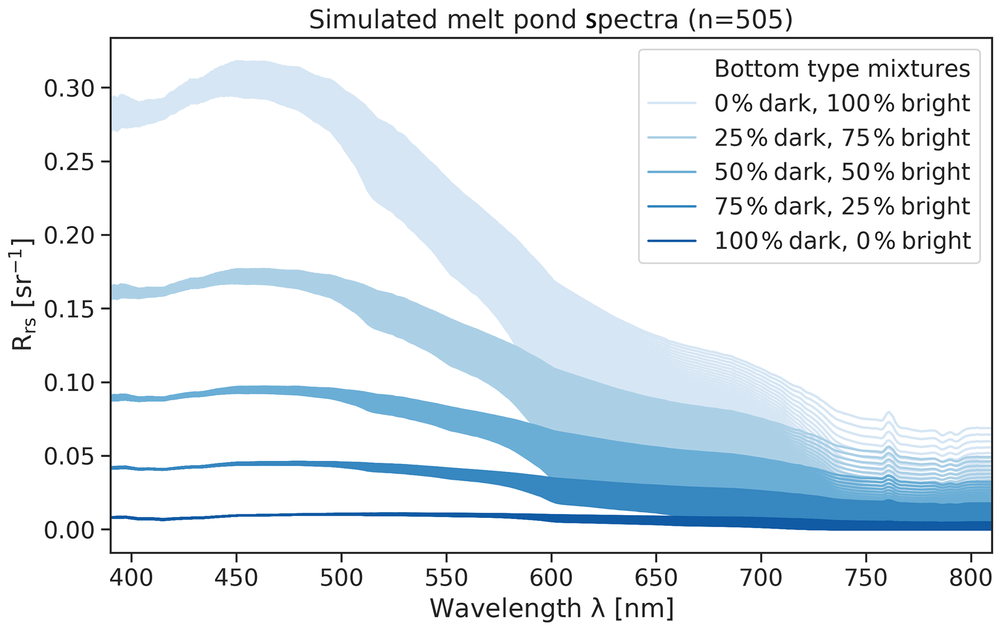
Figure 6 LUT generated with WASI-2D. Each of the five bottom type mixtures consists of 101 spectra (0 to 100 cm in 1 cm steps).

2.2.2 Data processing

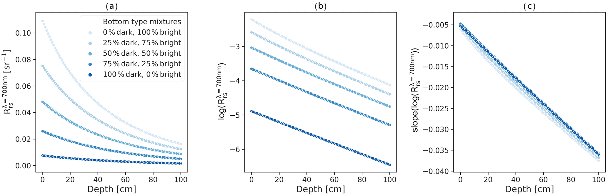
According to the Beer–Lambert law, the extinction of light at a certain wavelength in a medium is described by an exponential function. Here we assume that multiple scattering in meltwater and (multiple) reflections at the pond surface, bottom and sidewalls can be neglected to approximate the radiative transfer. Figure 7a illustrates the exponential decrease in R_rs with water depth at 700 nm for the five different bottom type mixtures. To linearize the effect, we computed the logarithm of the spectra (Fig. 7b). Lastly, we computed the first derivative of the logarithmized spectra (Fig. 7c) for each band by applying a Savitzky–Golay filter using a second-order polynomial fit on a 9 nm window (The Scipy community, 2019b).

Figure 7 Processing of spectral data exemplified for λ=700 nm.

We then computed Pearson's correlation coefficient (r) as (The Scipy community, 2019c)

$$\begin{array}{}\text{(5)}& {\displaystyle }{\displaystyle }r(x,y)={\displaystyle \frac{{\sum }_{i=\mathrm{0}}^{n-\mathrm{1}}(x_i-\stackrel{\mathrm{´}}{x})(y_i-\stackrel{\mathrm{´}}{y})}{\sqrt{{\sum }_{i=\mathrm{0}}^{n-\mathrm{1}}(x_i-\stackrel{\mathrm{´}}{x}{)}^{\mathrm{2}}{\sum }_{i=\mathrm{0}}^{n-\mathrm{1}}(y_i-\stackrel{\mathrm{´}}{y}{)}^{\mathrm{2}}}}},\end{array}$$

where x_i and $\stackrel{\mathrm{´}}{x}$ are the depth of the ith sample and the average depth, y_i and ý are the slope of the logarithmized reflectance at a certain wavelength of the ith sample and the average slope of the logarithmized reflectance at a certain wavelength, and n is the number of samples.

The orange curve in Fig. 8 illustrates the wavelength-dependent correlation coefficients of the slope of the logarithmized spectra and pond depths in the LUT. We observe an almost perfect negative correlation in bands between 700 and 750 nm. We performed the same processing for the simulated spectra as for the in situ pond spectra. The blue curve in Fig. 8 illustrates the wavelength-dependent correlation coefficients of measured pond depth and the slope of the logarithmized in situ spectra. We likewise observe strong negative correlations in the wavelength region around 700 nm.

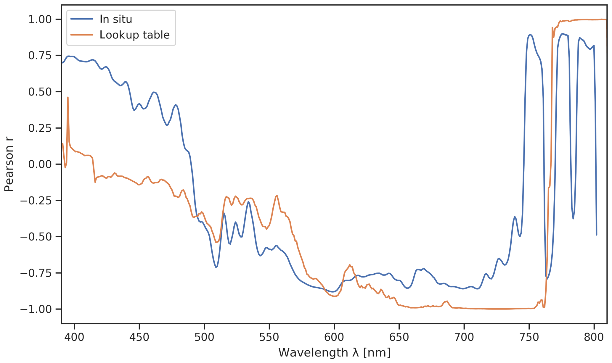
Figure 8 Wavelength-dependent correlation coefficients of pond depth with slope of log-scaled spectra for in situ measurements and simulated spectra.

To investigate the similarity of the dark and bright ice spectra, we normalized both bottom spectra at 710 nm and found a high spectral similarity between ∼590 and ∼800 nm (Fig. 9). Consequently, the slope of the logarithmized spectra is widely independent from the chosen bottom albedo in this wavelength region. Assuming that this also applies to ice spectra recorded under clear sky conditions, we used the Ibsen bare ice measurement to develop a model for clear sky conditions accordingly.

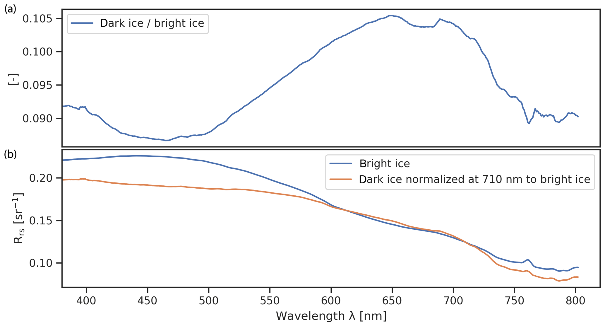
Figure 9 Quotient of bright and dark bare ice spectra (a) and R_rs of bright ice and dark ice normalized at 710 nm (b).

2.2.3 Linear model

Due to the strong negative correlation in the simulated as well as in the measured data, we chose the slope of the logarithmized spectrum at 710 nm ($r=-\mathrm{1.0}$ and −0.86 for simulated and in situ data, respectively) to develop a simple linear model. We used scikit-learn's LinearRegression function (Pedregosa et al., 2011) to fit a linear model to the simulated data with the Ibsen bare ice spectrum as bottom albedo using the method of ordinary least squares.

We found that the solar zenith angle affects the slope and y intercept of the linear model. Because the model should be applicable to a wide range of solar zenith angles, we implemented a second model to derive the slope and y intercept of the linear model for various solar zenith angles. We used WASI to generate spectral libraries for different solar zenith angles (0, 15, 30, 45, 60, 75, 90^∘) and found that the resulting change in slope and y intercept can each be described by an s-shaped curve. We used SciPy's optimize.curve_fit function (The Scipy community, 2019a) to fit generalized logistic functions (Richards, 1959) into the data. Using these functions, the model's slope and y intercept can be computed for different solar zenith angles (Fig. 10).

Figure 10 Change in model's y intercept and slope with solar zenith angle. Generalized logistic function fit into the simulated data.

The model is

$$\begin{array}{}\text{(6)}& {\displaystyle }{\displaystyle }z=a\left({\mathit{\theta }}_{\text{sun}}\right)+b\left({\mathit{\theta }}_{\text{sun}}\right){\left[{\displaystyle \frac{\partial \log R_{\text{rs}}\left(\mathit{\lambda }\right)}{\partial \mathit{\lambda }}}\right]}_{\mathit{\lambda }=\mathrm{710}\mathrm{nm}},\end{array}$$

where z is the predicted pond depth and θ_sun is the solar zenith angle. a and b are offset and slope as follows:

$$\begin{array}{}\text{(7)}& {\displaystyle }{\displaystyle }a\left({\mathit{\theta }}_{\text{sun}}\right)=-\mathrm{20.6}+{\displaystyle \frac{\mathrm{0.79}}{\mathrm{0.8}+\mathrm{5.8}\exp {\left(-\mathrm{0.13}\cdot {\mathit{\theta }}_{\text{sun}}\right)}^{\frac{\mathrm{1}}{\mathrm{2}}}}}\left(\mathrm{cm}\right)\end{array}$$

and

$$\begin{array}{ll}{\displaystyle }& {\displaystyle }b\left({\mathit{\theta }}_{\text{sun}}\right)=-\mathrm{1619.8}\\ \text{(8)}& {\displaystyle }& {\displaystyle }+{\displaystyle \frac{\mathrm{94}\mathrm{743.64}}{\mathrm{255.3}+\mathrm{7855}\exp {\left(-\mathrm{1.3}\cdot {\mathit{\theta }}_{\text{sun}}\right)}^{\frac{\mathrm{1}}{\mathrm{19.9}}}}}\left(\mathrm{cm}\right).\end{array}$$

We further computed the coefficient of determination (R²) as recommended by Kvålseth (1985) as

$$\begin{array}{}\text{(9)}& {\displaystyle }{\displaystyle }{R}^{\mathrm{2}}(y,\widehat{y})=\mathrm{1}-{\displaystyle \frac{{\sum }_{i=\mathrm{0}}^{n-\mathrm{1}}(y_i-{\widehat{y}}_i{)}^{\mathrm{2}}}{{\sum }_{i=\mathrm{0}}^{n-\mathrm{1}}(y_i-\stackrel{\mathrm{´}}{y}{)}^{\mathrm{2}}}},\end{array}$$

where y_i and ${\widehat{y}}_i$ are the true (simulated) and predicted values of the ith sample, n is the number of samples, and ${\stackrel{\mathrm{´}}{y}}_i=\frac{\mathrm{1}}{n}{\sum }_{i=\mathrm{0}}^{n-\mathrm{1}}{y}_i$ (Pedregosa et al., 2011; scikit-learn developers, 2018). In addition, we also computed the root mean square error (RMSE) as

$$\begin{array}{}\text{(10)}& {\displaystyle }{\displaystyle }\text{RMSE}(y,\widehat{y})=\sqrt{{\displaystyle \frac{\mathrm{1}}{n}}{\sum }_{i=\mathrm{0}}^{n-\mathrm{1}}(y_i-{\widehat{y}}_i{)}^{\mathrm{2}}}\end{array}$$

and the normalized RMSE (nRMSE) as

$$\begin{array}{}\text{(11)}& {\displaystyle }n\text{RMSE}(y,\widehat{y})={\displaystyle \frac{\text{RMSE}(y,\widehat{y})}{\stackrel{\mathrm{´}}{y}}}\cdot \mathrm{100}.\end{array}$$

For the model described above, we obtained a perfect correlation (r=1.0; probability value $p=\mathrm{8.9}\times {\mathrm{10}}^{-\mathrm{172}}$), an R² of 1.0 and an RMSE of 0.56 cm (nRMSE=1 %) on the simulated training data.

3 Results

We validated the model with the in situ melt pond dataset from dark and bright ponds (Sect. 2.1.2) and observed a strong linear and statistically significant correlation (r=0.86; $p=\mathrm{2.36}\times {\mathrm{10}}^{-\mathrm{15}}$; R²=0.65; RMSE=3.29 cm and nRMSE=19 %). Most of the points scatter along the 1:1 line except for one point whose actual depth is 10 cm and predicted depth is 18 cm (Fig. 11a). The externally studentized residual (t) (Kutner et al., 2004; Seabold and Perktold, 2010) classifies this point as an outlier (t>3), and therefore we excluded this point from the dataset. The removal of the outlier improves all performance measures (r=0.89; $p=\mathrm{4.34}\times {\mathrm{10}}^{-\mathrm{17}}$; R²=0.68; RMSE=3.11 cm; nRMSE=18 %). The slope of the line of best fit increases to 0.9686, and the intercept indicates an offset of 0.878 cm. If we further correct for the offset, R² increases to 0.74 and RMSE improves to 2.81 cm (nRMSE=16 %). The blue line is the line of best fit between actual and predicted pond depths. The linear equation of the line of best fit indicates that the model results in a small offset and a slope close to 1.0.

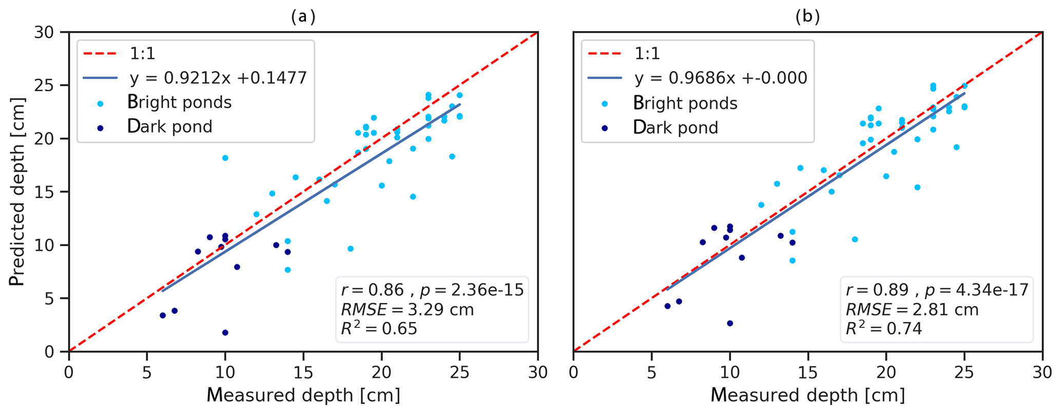
Figure 11 Measured versus predicted depth for the entire dataset (a) with outlier removed and offset correction (b).

4 Discussion

Our results show that a simple model based on the derivative of the log-scaled R_rs at 710 nm allows water depth retrieval of dark and bright melt ponds on Arctic sea ice. The model training on simulated data and the independent testing using in situ measurements prove the applicability of our approach.

4.1 Observational data

4.1.1 Spectral measurements

Measurements of albedo have a long tradition in Arctic research (e.g., Grenfell, 2004; Nicolaus et al., 2010; Perovich, 2002; Perovich and Polashenski, 2012) because albedo is an important quantity in climate models and can be measured with a single irradiance detector. In this study, we conducted measurements of R_rs because our model should be applicable to remote sensing data, and the quantity measured in optical remote sensing is radiance. It is only appropriate to derive an accurate radiance directly from the albedo of a Lambertian surface. This assumption, however, is not valid for specular water surfaces and may easily introduce errors. Morassutti and Ledrew (1996) identified changing E_d as the main error affecting reflectance data recording. To tackle this issue, we used a combination of two spectrometers described in Sect. 2.1.

Field spectroscopy is influenced by external factors and the measurement design itself. In contrast to ruler measurements, the spectrometer acquires information of an area. To ease comparison and limit the influence of spatial heterogeneities, we used a fore optic with a 1^∘ field of view to minimize the footprint (∼1 cm at a height of 60 cm). However, holding the instruments perfectly still for a period of several seconds is challenging, and even small changes in the position result in changes in the viewing angle, which increases the footprint of a measurement. For future campaigns, we therefore recommend using a gimbal to minimize the influence of roll and pitch of the handheld spectrometer setup. Another issue might have been reflections of the black spectrometer housings on the water surface possibly contributing to the offset between modeled and measured data.

Different refraction indices of wet and dry surfaces may cause part of the observed offset. Furthermore, using bottom albedos obtained from dry surfaces in WASI introduce a systematic offset. However, it remains unclear if the ice surface used to compute the spectral library was wet or dry.

Some of the scattering may be introduced by reflectances at the water surface, which we did not consider in the LUT computation because the necessary values for the parametrization are unknown. Another influence may be the different solar zenith angles between bare ice and pond measurements. The potential influence of the mentioned factors may be worth further examination to refine the model.

4.1.2 Pond depth measurements

Measuring the depth of a pond may appear trivial, but the bottom of a pond is frequently not flat and solid but can be slushy or riddled with holes. In addition, performing two measurements with a spectrometer and a folding ruler at the exact same location is difficult. We therefore recommend using a laser pointer at the end of the pole for orientation. These uncertainties explain some of the scattering in Fig. 11. Interpretation of field photographs of the pond bottoms, however, did not indicate any systematic errors associated with pond bottom characteristics.

4.2 Model validity

The majority of the field data used in this study are from bright blue ponds (n=38), while fewer measurements were obtained in dark ponds (n=11). We addressed this limited diversity of field data by computing a comprehensive LUT. The model generates accurate results (RMSE=2.81 cm) on the entire in situ test dataset and explains a large portion of its variability (R²=0.74). On the dataset from the dark pond, R² is less than 0 and nRMSE is 35 %. The reason is that measurements from the dark pond are very shallow (6–14 cm), and, thus, relative errors are larger compared to the deeper bright ponds. In addition, the number of data points is very small, and single outliers have a strong influence on performance metrics. The range of scattering around the 1:1 line (Fig. 11), however, is similar for the data from dark (RMSE=3.05 cm) and bright (RMSE=2.49 cm) ponds, proving that the model's accuracy is similar for both subsets.

The data used in this study are the most comprehensive set of R_rs and depth measurements from melt ponds on Arctic sea ice acquired under clear sky conditions. The dataset, however, originates from only three ponds, covering a limited variability of bottom characteristics and pond depth. More validation data are desirable to explore the model capabilities to derive pond depth from deep dark and shallow bright ponds, for pond depth >25 cm, and for a wider range of bottom types and solar zenith angles. In addition, more tests are necessary to explore how the model performs when the assumptions formulated in Sect. 2.2 are violated, e.g., when algae, suspended matter or yellow substances are abundant in the pond water or in the ice below the pond.

We successfully developed a model to accurately derive the depth of melt ponds on Arctic sea ice without having to consider the bottom ice characteristics of the pond; yet, we assume that we cannot entirely avoid any influence. When fitting a model to the Ocean Optics LUT (Fig. 7c), we observe scattering around the 1:1 line resulting in an RMSE of 1.88 cm (nRMSE=4 %). In the Ocean Optics LUT, however, the only variable parameter is bottom type mixture; we therefore conclude that the scattering results from the difference in bottom albedo. Consequently, bottom albedo may affect the model, which may explain some of the scattering in the test data.

Optical satellite data can only be obtained under clear sky conditions, but remote sensing images are likewise acquired from helicopters and unmanned aerial vehicles. These platforms also operate under diffuse illumination conditions, which are frequent in the Arctic. To check the validity of the model for overcast conditions, we applied the clear sky model to data from the same area acquired on 14 June 2017 during diffuse illumination conditions. The performance, however, is low (Fig. 12) and shows a moderate correlation (r=0.64; $p=\mathrm{2.6}\times {\mathrm{10}}^{-\mathrm{4}}$), an R²<0 and an RMSE of 12.76 cm (nRMSE=63 %). We attribute the low performance to the different illumination conditions. Under diffuse conditions, a considerable part of the reflectance measured above the water surface is due to the reflection of clouds at the water surface. Further, the optical path length of the incoming light in water changes under overcast conditions.

We therefore conclude that the present model is only valid for clear sky conditions. The model accounts for the influence of varying solar zenith angles, but field data were limited to solar zenith angles between 58.9 and 61^∘. To enlarge its validity range, more field data covering different weather and illumination conditions are necessary.

Figure 12 Measured versus predicted water depth for data acquired under overcast conditions on 14 June 2017.

5 Conclusions

We present a linear model slope-based approach in the spectral region around 710 nm to retrieve the depth of melt ponds on Arctic sea ice. However, the model is not restricted to Arctic sea ice and may be tested in shallow supraglacial ponds as well. The model calibration on simulated data and independent validation on in situ data prove the applicability and robustness of our approach. The final model is valid for hyperspectral data (R_rs) acquired under clear sky conditions and addresses varying solar zenith angles.

We used WASI to generate a LUT of pond spectra for five different bottom albedos and pond depths between 0 and 100 cm assuming clear pond water. We found that the slope of the log-scaled R_rs at 710 nm is widely independent from the bottom albedo and highly correlated with pond depth. Thus, we applied a linear model to retrieve pond depth from R_rs in this wavelength region. The slope and y intercept of the linear equation, however, change with the solar zenith angle for which other models do not account for (e.g., Legleiter et al., 2014; Tedesco and Steiner, 2011). To overcome this limitation, we trained linear models for seven solar zenith angles in between and found that a general logistic function is able to describe the change in slope and y intercept for each solar zenith angle. The inputs for our model, therefore, are the slope of the log-scaled $R_{\text{rs}}^{\mathit{\lambda }=\mathrm{710}}$ and sun zenith angle. We successfully validated the model on in situ measurements (r=0.89; R²=0.74; RMSE=2.81 cm; nRMSE=16 %) with solar zenith angles between 58.9 and 61^∘ and observed similar accuracies for bright and dark ponds.

The next step is the transfer to hyperspectral airborne and satellite systems, e.g., EnMAP (Guanter et al., 2016), to enable a synoptic view on the evolution of melt ponds on Arctic sea ice. One constraint may be the size of melt ponds, which requires a high spatial resolution. We further assume that the additive signals of the atmosphere and reflections of skylight at the water surface may complicate the retrieval of pond depth with remote sensors. In addition, the sensitivities and band settings of remote sensors also affect the transferability of our approach. Here, further testing and comprehensive ground truth data are necessary. In these regards, we expect the Multidisciplinary drifting Observatory for the Study of Arctic Climate (MOSAiC) expedition to result in further improvements.