Landfast sea ice material properties derived from ice bridge simulations using the Maxwell elasto-brittle rheology

The Maxwell elasto-brittle (MEB) rheology is implemented in the Eulerian finite-difference (FD) modeling framework commonly used in classical viscous-plastic (VP) models. The role of the damage parameterization, the cornerstone of the MEB rheology, in the formation and collapse of ice arches and ice bridges in a narrow channel is investigated. Ice bridge simulations are compared with observations to derive constraints on the mechanical properties of landfast sea ice. Results show that the overall dynamical behavior documented in previous MEB models is reproduced in the FD implementation, such as the localization of the damage in space and time and the propagation of ice fractures in space at very short timescales. In the simulations, an ice arch is easily formed downstream of the channel, sustaining an ice bridge upstream. The ice bridge collapses under a critical surface forcing that depends on the material cohesion. Typical ice arch conditions observed in the Arctic are best simulated using a material cohesion in the range of 5–10 kN m⁻². Upstream of the channel, fracture lines along which convergence (ridging) takes place are oriented at an angle that depends on the angle of internal friction. Their orientation, however, deviates from the Mohr–Coulomb theory. The damage parameterization is found to cause instabilities at large compressive stresses, which prevents the production of longer-term simulations required for the formation of stable ice arches upstream of the channel between these lines of fracture. Based on these results, we propose that the stress correction scheme used in the damage parameterization be modified to remove numerical instabilities.

1 Introduction

The term landfast ice designates sea ice that is attached to the coastlines, acting as an immobile and seasonal extension of the land. It starts to form in shallow water in the early stages of the Arctic freeze-up (Barry et al., 1979; Reimnitz et al., 1978) and grows throughout the Arctic winter, usually reaching its maximum extent in early spring (Yu et al., 2014). Typically, large landfast ice areas can form and remain stable due to the presence of islands or via the grounding of ice keels on the ocean floor (Reimnitz et al., 1978; Mahoney et al., 2007; Selyuzhenok et al., 2017). Where the water is too deep for grounding, landfast ice can also form where ice floes are jammed in narrow passages between islands or pieces of grounded ice. In the Canadian Arctic Archipelago (CAA), this type of ice is referred to as landlocked. The resulting ice bridges, also called ice arches for their characteristic arching edges (Fig. 1), can have a profound influence on sea ice circulation, via the closure of gateways (Melling, 2002; Kwok, 2005), and on regional hydrography, via the formation of winter polynyas downstream of the arches (Barber and Massom, 2007; Dumont et al., 2010; Shroyer et al., 2015). Most studies about ice arches focus on the Nares Strait (Fig. 1) and Lincoln Sea ice bridges (Kozo, 1991; Dumont et al., 2008; Dansereau et al., 2017; Moore and McNeil, 2018; Vincent, 2019), which affect the export of thick multi-year ice into Baffin Bay (Kwok and Cunningham, 2010; Ryan and Münchow, 2017). Ice arches, however, are a seasonal feature in several locations of the Canadian Arctic Archipelago (Marko and Thomson, 1977; Sodhi, 1997; Melling, 2002) and are also present in the Kara and Laptev seas (Divine et al., 2004; Selyuzhenok et al., 2015; Olason, 2016), where they play a role in the formation of extensive landfast ice covers.

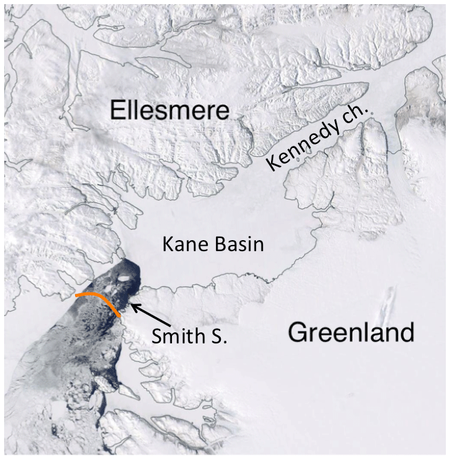
Figure 1 NASA Worldview image of a stable landfast ice arch in Nares Strait, from Moderate Resolution Imaging Spectroradiometer (MODIS)-corrected reflectance imagery (true color), on 1 May 2018. The orange curve indicates the position of the stable ice in Dansereau et al. (2017).

Despite decades of observations (Melling, 2002; Kwok, 2005; Moore and McNeil, 2018; Ryan and Münchow, 2017), the formation, persistence and breakup of ice arches remain difficult to predict. It is, however, clear from modeling studies that the ability of sea ice to form arches relates to the material properties of sea ice. A number of studies showed that ice arches are produced if the rheology includes sufficient material cohesion (Ip, 1993; Hibler et al., 2006; Dumont et al., 2008). Using the ellipse yield curve of Hibler (1979), this can be achieved either by decreasing the yield curve ellipse aspect ratio (Kubat et al., 2006; Dumont et al., 2008) or by extending the ellipse towards larger isotropic tensile strength (Beatty and Holland, 2010; Olason, 2016; Lemieux et al., 2016). The range of parameter values that are appropriate for the production of ice bridges varies between different numerical studies, suggesting that different forcing or model implementations may influence the ice arch formation (Olason, 2016; Lemieux et al., 2016, 2018).

In recent years, new rheologies were proposed to reproduce the observed characteristics of ice failure, such as the preferred orientation of the lines of fracture (Wilchinsky and Feltham, 2004; Schreyer et al., 2006) or the brittle behavior of sea ice at small scales (Girard et al., 2011; Dansereau et al., 2016). Among this effort, a brittle damage parameterization (Amitrano et al., 1999) was implemented in the neXtSIM model (Rampal et al., 2016), as part of the elasto-brittle (Girard et al., 2011, EB) and Maxwell elasto-brittle (Dansereau et al., 2016, MEB) rheologies. The MEB rheology was shown to produce ice arches in the Nares Strait region that remain stable for several days, and arch fractures that are part of the landfast ice breakup process (Dansereau et al., 2017). The simulated stable ice arches in Dansereau et al. (2017) are located downstream of either Smith Sound or Kennedy channel (see the orange curve in Fig. 1). These locations differ from the observed ice arch positions in Nares Strait upstream of these channels (see, e.g., Fig. 1) or in the Lincoln Sea (Vincent, 2019), which are well reproduced by standard VP or elastic viscous-plastic (EVP) models (e.g., Dumont et al., 2008; Rasmussen et al., 2010). Whether this difference in behavior stems from the different physics of MEB and VP rheologies or it is just due to the different numerical framework used in both models remains an open question.

The EB and MEB models have so far been implemented using Lagrangian advection schemes and/or finite-element methods (e.g., Rampal et al., 2016; Dansereau et al., 2017). These numerical features, however, make it difficult to compare the different MEB and EB physics with that of the standard VP or EVP rheologies of the modeling community, as these are usually implemented on Eulerian finite-difference (FD) numerical frameworks. In this paper, we present our implementation of the MEB rheology on the FD numerical framework of the McGill VP sea ice model (Tremblay and Mysak, 1997; Lemieux et al., 2008, 2014). To our knowledge, it is the first time the MEB rheology has been implemented on the numerical platform of a VP model such that its different physics can be assessed independently from the numerical implementation. With this model, we investigate the role of the damage parameterization and the material strength parameters in the formation of ice arches, using an idealized model domain capturing the basic features of real-life geometries where ice arches are observed. We also identify a numerical issue associated with the damage parameterization, which significantly impacts long simulations.

The paper is organized as follows. In Sect. 2, we present the implementation of the Maxwell elasto-brittle rheology in our FD numerical framework. A detailed analysis of the breakup of the ice bridge simulated by the MEB rheology is presented in Sect. 3, along with a sensitivity analysis of the results with respect to the material parameters. The MEB model performance in simulating compressive fractures is discussed in Sect. 4, with summarized conclusions in Sect. 5.

2 Maxwell elasto-brittle model

2.1 Momentum and continuity equations

The 2D momentum equation describing the motion of sea ice is written as follows:

$$\begin{array}{}\text{(1)}& {\mathit{\rho }}_{\mathrm{i}}h{\displaystyle \frac{\partial \mathit{u}}{\partial t}}=\mathrm{\nabla }\cdot \mathit{\sigma }+\mathit{\tau },\end{array}$$

where ρ_i is the ice density, h is the mean ice thickness, u ($=u\widehat{\mathbf{i}}+v\widehat{\mathbf{j}}$) is the ice velocity vector, σ is the vertically integrated internal stress tensor, and τ ($={\mathit{\tau }}_{\mathrm{a}}+{\mathit{\tau }}_{\mathrm{w}}$) is the total external surface forcings from winds and ocean currents. Note that we write the momentum equation in terms of the vertically integrated internal sea ice stresses (i.e., ∇⋅σ) as standard in VP models (e.g., Hibler, 1979; Hunke and Dukowicz, 1997; Wilchinsky and Feltham, 2004), as opposed to the mean internal sea ice stresses (i.e., ∇⋅σ) used in previous implementations of the MEB rheology (Dansereau et al., 2016; Rampal et al., 2016). We assume no grounding of ice on the ocean floor and neglect the Coriolis term. This omission is appropriate for landfast ice but can result in small errors in drifting ice (Turnbull et al., 2017). The advection of momentum (which scales as ρ_iH[U]²∕L, where H, [U] and L are the characteristic ice thickness, velocity, and length scales) is 3 orders of magnitude smaller than characteristic air or ocean surface stresses (Zhang and Hibler, 1997; Hunke and Dukowicz, 1997). At the edge of an ice arch where a discontinuity in sea ice drift is present at the grid scale (2 km in our case), it remains 2 orders of magnitude smaller than other terms in the momentum equation.

The total surface stress is defined in terms of an effective stress (τ_LFI) that represents the combined wind and ocean forces acting on the landfast ice and an additional water drag term that only acts on the drifting ice. That is, using the standard bulk formula (with air and water turning angles set to zero,  McPhee, 1979), we have the following equations:

$$\begin{array}{}\text{(2)}& {\displaystyle }\mathit{\tau }& {\displaystyle }={\mathit{\rho }}_{\mathrm{a}}{C}_{\mathrm{da}}\left|{\mathit{u}}_{\mathrm{a}}\right|{\mathit{u}}_{\mathrm{a}}+{\mathit{\rho }}_{\mathrm{w}}{C}_{\mathrm{dw}}|{\mathit{u}}_{\mathrm{w}}-\mathit{u}|({\mathit{u}}_{\mathrm{w}}-\mathit{u}),\text{(3)}& {\displaystyle }& {\displaystyle }\approx {\mathit{\rho }}_{\mathrm{a}}{C}_{\mathrm{da}}\left|{\mathit{u}}_{\mathrm{a}}\right|{\mathit{u}}_{\mathrm{a}}-{\mathit{\rho }}_{\mathrm{w}}{C}_{\mathrm{dw}}\left|{\mathit{u}}_{\mathrm{w}}\right|{\mathit{u}}_{\mathrm{w}}-{\mathit{\rho }}_{\mathrm{w}}{C}_{\mathrm{dw}}\left|\mathit{u}\right|\mathit{u},\text{(4)}& {\displaystyle }& {\displaystyle }\approx {\mathit{\tau }}_{\mathrm{LFI}}-{\mathit{\rho }}_{\mathrm{w}}{C}_{\mathrm{dw}}\left|\mathit{u}\right|\mathit{u},\end{array}$$

where ρ_a and ρ_w are the air and water densities, C_da and C_dw are the air and water drag coefficients (see values in Table 2), and u_a and u_w are the surface air and water velocities. Note that the cross terms u_wu have been neglected. This equation is therefore exact for landfast ice, the focus of this study, and constitutes an approximation only for ice drifting over an ocean current. Below, we specify τ_LFI and give the characteristic wind speed and ocean current equivalent to this forcing for reference.

The continuity equations used for the temporal evolution of the mean ice thickness h (volume per grid cell area) and concentration A ($\mathrm{0}<A<\mathrm{1}$) are written as follows:

$$\begin{array}{}\text{(5)}& {\displaystyle }& {\displaystyle \frac{\partial h}{\partial t}}+\mathrm{\nabla }\cdot \left(h\mathit{u}\right)=S_h,\text{(6)}& {\displaystyle }& {\displaystyle \frac{\partial A}{\partial t}}+\mathrm{\nabla }\cdot \left(A\mathit{u}\right)=S_A,\end{array}$$

where S_h and S_A are thermodynamic sink and source terms for ice thickness and compactness, respectively. As we are only interested in the dynamical behavior of the sea ice model, all thermodynamics are turned off so that S_h=0 and S_A=0. Mechanical redistribution (i.e., ridging) is taken into account by capping the ice concentration at 1 % (or 100 %) in convergence. As the mean ice thickness h is allowed to grow, the capping increases the actual ice thickness (Schulkes, 1995).

Langleben (1962)Weeks and Assur (1967)Tabata (1955)Weeks and Assur (1967)Tabata (1955)Tabata (1955)Weeks and Assur (1967)Sukhorukov (1996)Hata and Tremblay (2015b)Schulson et al. (2006)Weiss et al. (2007)Weiss et al. (2007)Tremblay and Hakakian (2006)Tucker and Perovich (1992)Richter-Menge et al. (2002)Richter-Menge and Elder (1998)Weiss et al. (2007)Tremblay and Hakakian (2006)Tucker and Perovich (1992)Richter-Menge and Elder (1998)Sodhi (1997)Weiss et al. (2007)

Table 1 Material strength parameters from observations.

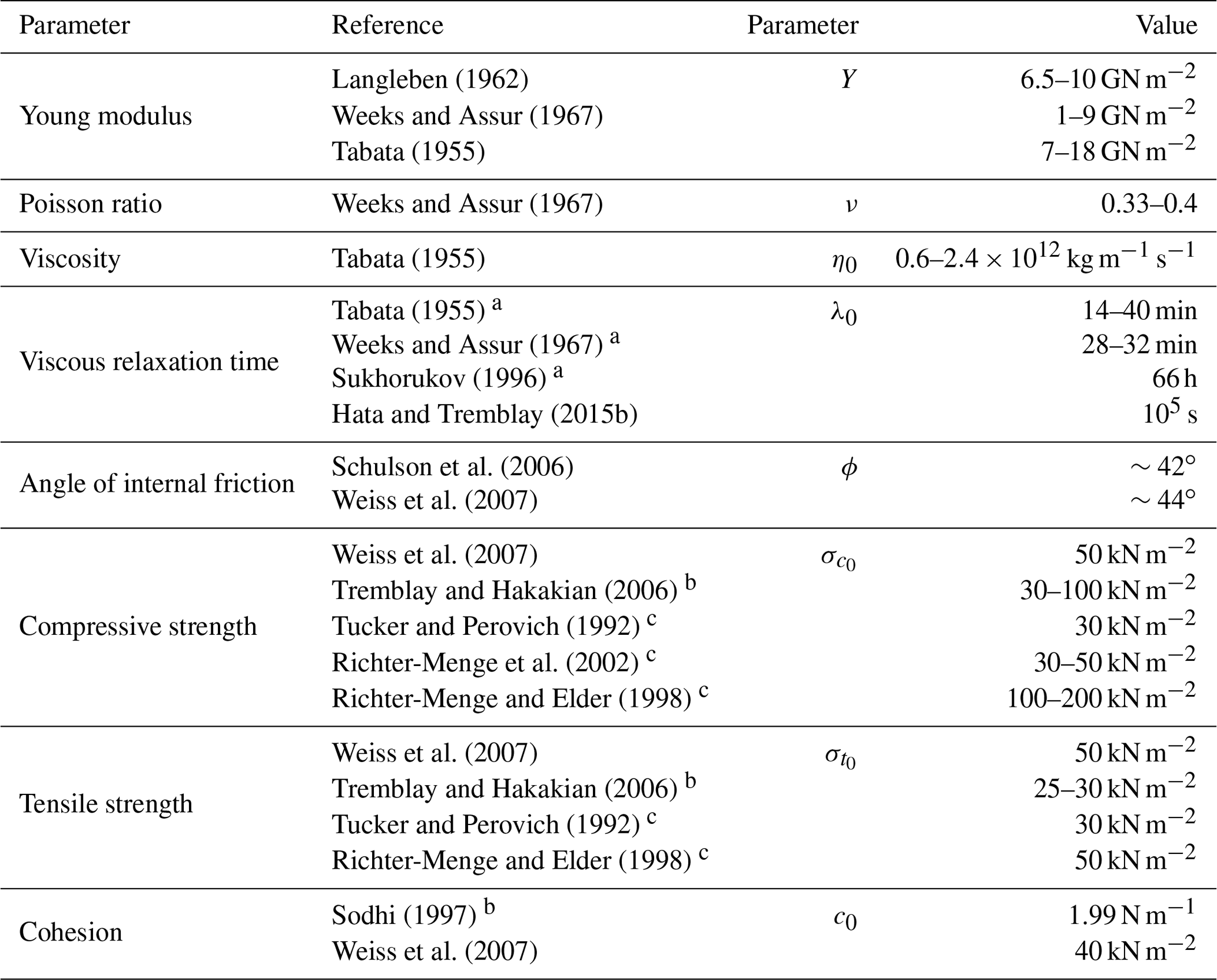
^a From small-scale measurements in the field. ^b Estimate from satellite observations. ^c Observed peak stresses.

2.2 Rheology

2.2.1 Visco-elastic regime

Following Dansereau et al. (2016), we consider the ice as a visco-elastic brittle material behaving like a stiff spring and strong dashpot in series if the stresses are relatively small. The corresponding stress–strain relation is that of a Maxwell visco-elastic material:

$$\begin{array}{}\text{(7)}& {\displaystyle \frac{\partial \mathit{\sigma }}{\partial t}}+{\displaystyle \frac{\mathrm{1}}{\mathit{\lambda }}}\mathit{\sigma }=E\mathbf{C}:\dot{\mathit{ϵ}},\end{array}$$

where λ is the viscous time relaxation ($\mathit{\lambda }=\frac{\mathit{\eta }}{E}$, η being the vertically integrated viscosity), E is the vertically integrated elastic stiffness, C is the elastic modulus tensor and “:” denotes the double dot product of tensors. In generalized matrix form, the tensors C and $\dot{\mathit{ϵ}}$ are written as follows:

$$\begin{array}{}\text{(8)}& \mathbf{C}={\displaystyle \frac{\mathrm{1}}{\mathrm{1}-{\mathit{\nu }}^{\mathrm{2}}}}\left(\begin{array}{ccc}\mathrm{1}& \mathit{\nu }& \mathrm{0}\\ \mathit{\nu }& \mathrm{1}& \mathrm{0}\\ \mathrm{0}& \mathrm{0}& \mathrm{1}-\mathit{\nu }\end{array}\right)=\left(\begin{array}{ccc}{C}_{\mathrm{1}}& C_{\mathrm{2}}& \mathrm{0}\\ C_{\mathrm{2}}& C_{\mathrm{1}}& \mathrm{0}\\ \mathrm{0}& \mathrm{0}& C_{\mathrm{3}}\end{array}\right)\end{array}$$

$$\begin{array}{}\text{(9)}& \left(\begin{array}{r}{\dot{\mathit{ϵ}}}_{\mathrm{11}}\\ {\dot{\mathit{ϵ}}}_{\mathrm{22}}\\ {\dot{\mathit{ϵ}}}_{\mathrm{12}}\end{array}\right)=\left(\begin{array}{c}\frac{\partial u}{\partial x}\\ \frac{\partial v}{\partial y}\\ \frac{\mathrm{1}}{\mathrm{2}}(\frac{\partial u}{\partial y}+\frac{\partial v}{\partial x}).\end{array}\right),\end{array}$$

where ν (=0.33) is the Poisson ratio. The components of the elastic modulus tensor C are derived using the plane stress approximation (i.e., following the original assumption that the vertical stress components are negligible; see Rice, 2010). Note that we neglect the advection of stress in the time derivative of Eq. (7) as we focus on landfast ice.

The visco-elastic regime of the MEB model (before fracture) is dominated by a fast and reversible elastic response (first term on the left-hand side of Eq. 7), with a slow viscous dissipation acting over longer timescales (second term on the left-hand side). The reversibility of the elastic deformations implies that the elastic strains return to zero if all loads are removed. This results from a memory of the previous elastic stress and strain states given by the time derivative in Eq. (7). The Maxwell viscosity term, although orders of magnitude lower than the other terms in the visco-elastic regime, leads to a slow viscous dissipation of this elastic stress memory over long timescales determined by λ (days in our case).

While Eq. (7) is similar in form to the stress–strain relationship of the EVP model (Hunke, 2001), the elastic component in the EVP model was introduced to improve the computational efficiency of the VP model by allowing for an explicit numerical scheme and efficient parallelization (Hunke and Dukowicz, 1997). In the MEB model, the elastic component represents the elastic behavior of sea ice, while the viscous relaxation component is introduced to dissipate the elastic strains into permanent deformations. The use of a viscous component is consistent with the observation of viscous creep (Tabata, 1955; Weeks and Assur, 1967) and viscous relaxation in field experiments (Tucker and Perovich, 1992; Sukhorukov, 1996; Hata and Tremblay, 2015b). The viscous relaxation term is also analogous to the viscous term in the thermal stress models of Lewis (1993) and Hata and Tremblay (2015a).

2.2.2 Damage parameterization

In the MEB model, the brittle fracture is simulated using a damage parameterization, which is based on progressive damage models originally developed in the field of rock mechanics to reproduce the nonlinear (brittle) behavior in rock deformation and seismicity (Cowie et al., 1993; Tang, 1997; Amitrano and Helmstetter, 2006). In these models, the material damage associated with microcracking is simulated by altering the material properties (e.g., the Young modulus or the material strength) at the model element (or local) scale. If heterogeneity is present in the material, the damage parameterization simulates the self-organization of the microcracks in a macroscopic line of fracture, as observed in laboratory experiments. It was first used for large-scale sea ice modeling by Girard et al. (2011) and is now implemented in the Lagrangian dynamic–thermodynamic sea ice model neXtSIM (Rampal et al., 2019).

The sea ice deformations associated with the brittle fractures are parameterized by a gradual decrease in the elastic stiffness E and viscosity η at the local scale, and consequently as a local increase in the magnitude of the deformation associated with a given stress state. The local increase in deformations results in the concentration of internal stresses in adjacent grid cells, leading to the propagation of the fractures in space. The decrease in elastic stiffness and viscosity is set by a damage parameter d representing the weakening of the ice upon fracturing (Bouillon and Rampal, 2015). The damage parameter has a value of 0 for undamaged sea ice and 1 for fully damaged ice.

The damage increases when the stress state exceeds a critical stress, defined by the Mohr–Coulomb criterion. This yield criterion is standard for granular materials and in agreement with laboratory experiments (Schulson et al., 2006) and field observations (Weiss et al., 2007). We also investigate the use of a compressive cutoff to limit the uniaxial compression (${\mathit{\sigma }}_{\mathrm{2}}={\mathit{\sigma }}_{\mathrm{I}}-{\mathit{\sigma }}_{\mathrm{II}}$; see Fig. 2). In terms of the stress invariants σ_I and σ_II, this can be written as follows:

$$\begin{array}{}\text{(10)}& F\left(\mathit{\sigma }\right)=\left\{\begin{array}{rl}& {\mathit{\sigma }}_{\mathrm{II}}+\mathit{\mu }{\mathit{\sigma }}_{\mathrm{I}}-c<\mathrm{0}\\ & \text{Mohr–Coulomb}\\ & {\mathit{\sigma }}_{\mathrm{I}}-{\mathit{\sigma }}_{\mathrm{II}}>{\mathit{\sigma }}_{\mathrm{c}}h{e}^{-C(\mathrm{1}-A)}\\ & \text{compression cutoff}\end{array}\right.,\end{array}$$

where

$$\begin{array}{}\text{(11)}& {\displaystyle }& {\displaystyle }c=c_{\mathrm{0}}h{e}^{-a(\mathrm{1}-A)},\text{(12)}& {\displaystyle }& {\displaystyle }{\mathit{\sigma }}_{\mathrm{c}}={\mathit{\sigma }}_{{\mathrm{c}}_{\mathrm{0}}}h{e}^{-a(\mathrm{1}-A)}.\end{array}$$

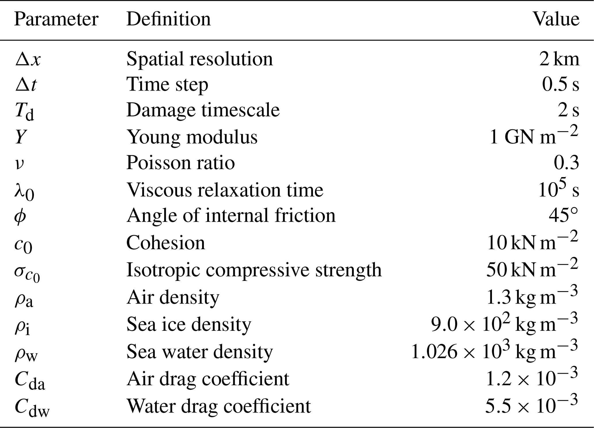
where σ_I is the isotropic normal stress (defined as negative in compression), σ_II is the maximum shear stress, c is the vertically integrated cohesion, μ (=sin ϕ) is the coefficient of internal friction of ice, ϕ is the angle of internal friction and σ_c is the vertically integrated uniaxial compressive strength. The parameterization of c and σ_c follows the form of the internal sea ice pressure in the standard VP model with the ice concentration parameter a set to 20 (Hibler, 1979). The cohesion c₀ and compressive strength ${\mathit{\sigma }}_{{\mathrm{c}}_{\mathrm{0}}}$ are the material properties derived from in situ observations (see Table 1 for values and references) and laboratory experiments (Timco and Weeks, 2010). Model parameters used in this and other studies are listed in Tables 2 and 3.

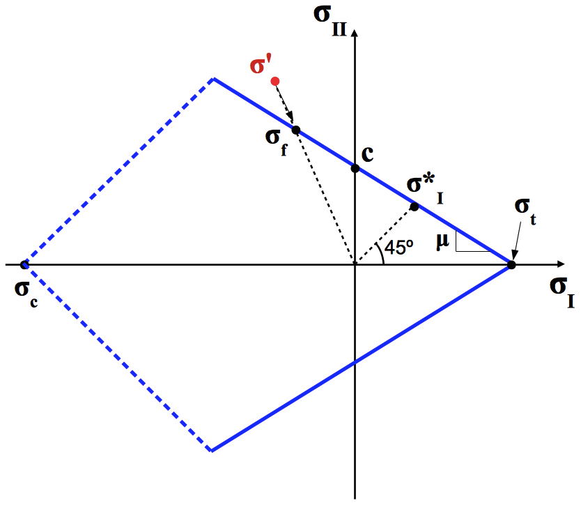
Figure 2 Yield criterion (Mohr–Coulomb and compressive cutoff) in stress invariant space (σ_I, σ_II) with following the mechanical strength parameters: compressive strength (σ_c), cohesion (c), coefficient of internal friction (μ=sin ϕ, ϕ being the angle of internal friction), isotropic tensile strength (σ_t) and uniaxial tensile strength (${\mathit{\sigma }}_{\mathrm{I}}^{*}$, where the second principal stress invariant σ₂ is zero or ${\mathit{\sigma }}_{\mathrm{I}}={\mathit{\sigma }}_{\mathrm{II}}={\mathit{\sigma }}_{\mathrm{I}}^{*}$). The stress before and after the correction (see Eq. 13) is denoted by σ^′, and σ_f, respectively. The correction from σ^′ to σ_f is done following a line going through the origin.

Following Rampal et al. (2016), the introduction of damage upon failure is proportional to the local stress in excess of the yield criterion. A damage factor Ψ ($\mathrm{0}<\mathrm{\Psi }<\mathrm{1}$) is used to scale the stress back on the yield curve. It is defined as follows (see Appendix A for the derivation Ψ):

$$\begin{array}{}\text{(13)}& {\mathit{\sigma }}_f=\mathrm{\Psi }{\mathit{\sigma }}^{\prime }\text{with}\mathrm{\Psi }=min\left(\mathrm{1},{\displaystyle \frac{c}{{\mathit{\sigma }}_{\mathrm{II}}^{\prime }+\mathit{\mu }{\mathit{\sigma }}_{\mathrm{I}}^{\prime }}},{\displaystyle \frac{{\mathit{\sigma }}_{\mathrm{c}}}{{\mathit{\sigma }}_{\mathrm{I}}^{\prime }-{\mathit{\sigma }}_{\mathrm{II}}^{\prime }}}\right),\end{array}$$

where σ_f is the corrected stress lying on the yield curve and σ^′ is the prior stress state that exceeds the yield criterion. Note that the stress components are all scaled by the same damage factor, such that the path of the stress correction in stress invariant space follows a line from the uncorrected stress state to the origin (see Fig. 2). The stress correction path does not correspond to a flow rule: the magnitude of the excess stress is only used to increase the damage parameter. It determines the magnitude of the strain associated with a stress state but otherwise does not change the visco-elastic relationship in Eq. (7).

Table 2 Default model parameters.

The temporal evolution of the damage parameter follows a simple relaxation with a damage timescale T_d (Dansereau et al., 2016):

$$\begin{array}{}\text{(14)}& {\displaystyle \frac{\partial d}{\partial t}}={\displaystyle \frac{(\mathrm{1}-\mathrm{\Psi })(\mathrm{1}-d)}{T_{\mathrm{d}}}},\end{array}$$

where T_d is set to the advective timescale associated with the propagation of elastic waves in undamaged ice (i.e., $T_{\mathrm{d}}=\mathrm{\Delta }x/c_{\mathrm{e}}$, Δx being the spatial resolution of the model and c_e the elastic wave speed). Consequently, the damage at any given time is a function of the previously accumulated damage. No damage healing process was included in this study as we focus on the breakup of ice bridges at small timescales. For the same reason, the advection of damage is neglected. The relaxation timescale ($T_{\mathrm{d}}/(\mathrm{\Psi }-\mathrm{1})$) in Eq. (14) is time step dependent via its dependency on the damage factor Ψ. That is, a larger time step yields larger stress increments and larger excess stresses at each time level, decreasing the timescale for the damage relaxation. The sensitivity of the damage parameterization on the model time step led Dansereau et al. (2016) to suggest that the model time step be set to exactly T_d, otherwise the damage could travel faster than the elastic waves. We argue that while this point is true when using a fixed damage reduction parameter (as in Amitrano et al., 1999; Girard et al., 2011), the use of a damage factor Ψ relates the damage parameter to the rate of changes in the stress state, which is associated with the propagation of elastic waves. The propagation of damage in space is thus bounded by the elastic wave speed, and a smaller time step (0.5 s in this study) should be used to respect the Courant–Friedrichs–Lewy (CFL) criterion associated to the elastic waves.

The elastic stiffness E and Maxwell viscosity η are written as a nonlinear function of d, with a dependency on the ice thickness and sea ice concentration inspired by the ice strength parameterization of Hibler (1979):

$$\begin{array}{}\text{(15)}& {\displaystyle }& {\displaystyle }E=Yh{e}^{-a(\mathrm{1}-A)}(\mathrm{1}-d),\text{(16)}& {\displaystyle }& {\displaystyle }\mathit{\eta }={\mathit{\eta }}_{\mathrm{0}}h(\mathrm{1}-d{)}^{\mathit{\alpha }},\end{array}$$

where Y (=1 GN m⁻², smaller than in Bouillon and Rampal, 2015, and similar to Dansereau et al., 2016; see Table 3) is the Young modulus of undeformed sea ice, η₀ is the viscosity of undeformed sea ice and α is an integer set to 4 that determines the smoothness of the transition from visco-elastic behavior to the post-fracture viscous behavior (Dansereau et al., 2016). Note that E and η are defined as in previous implementations except for the linear dependence in ice thickness required because of the use of vertically integrated stress σ.

Hunke (2001)Bouillon and Rampal (2015)Dansereau et al. (2016)Sulsky and Peterson (2011)Tran et al. (2015)Olason (2016)Dansereau et al. (2016)Hunke (2001)Tremblay and Mysak (1997)Hibler (1979)Dumont et al. (2008)Tran et al. (2015)Sulsky and Peterson (2011)Lemieux et al. (2016)Olason (2016)Dansereau et al. (2016)Hunke (2001)Dumont et al. (2008)Bouillon and Rampal (2015)Tremblay and Mysak (1997)Hibler (1979)Hibler (1979)Hunke (2001)Dumont et al. (2008)Lemieux et al. (2016)Olason (2016)Dansereau et al. (2016)Olason (2016)Tran et al. (2015)Sulsky and Peterson (2011)Bouillon and Rampal (2015)Olason (2016)Lemieux et al. (2016)Beatty and Holland (2010)Dansereau et al. (2016)Tran et al. (2015)Sulsky and Peterson (2011)Bouillon and Rampal (2015)

Table 3 Material properties used in sea ice models (VP, EVP and MEB).

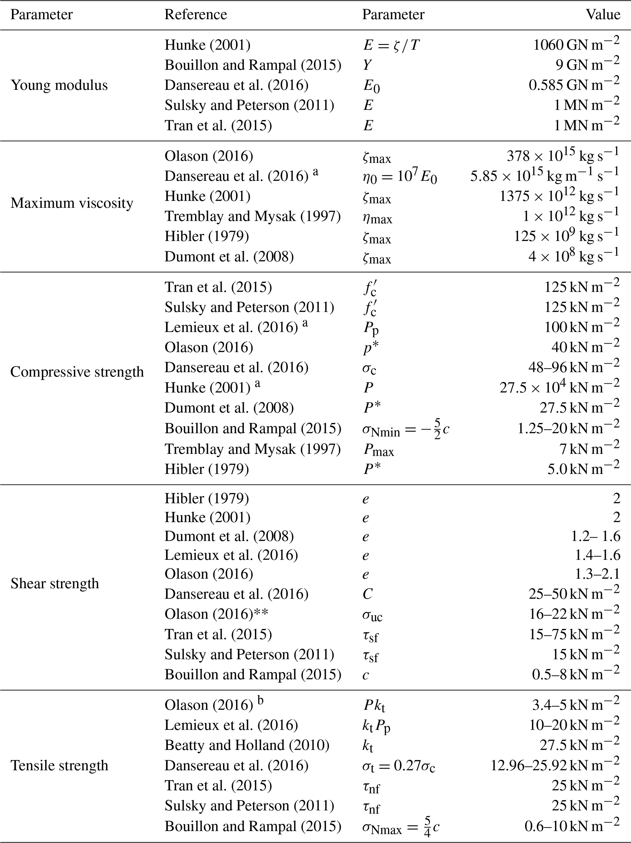
^a For 1 m thick ice. ^b Using the Mohr–Coulomb curve with ϕ=45^∘.

The relaxation time constant λ in Eq. (7) is then written as follows:

$$\begin{array}{}\text{(17)}& \mathit{\lambda }={\displaystyle \frac{\mathit{\eta }}{E}}={\displaystyle \frac{{\mathit{\lambda }}_{\mathrm{0}}(\mathrm{1}-d{)}^{\mathit{\alpha }-\mathrm{1}}}{e^{-a(\mathrm{1}-A)}}},\end{array}$$

where λ₀ ($={\mathit{\eta }}_{\mathrm{0}}/Y={\mathrm{10}}^{\mathrm{5}}$ s, smaller than in Dansereau et al., 2016, but in agreement with observations; see Table 1) is a parameter that corresponds to the viscous relaxation timescale in undamaged sea ice. In the limit when λ₀ tends to infinity, the MEB rheology tends to the elasto-brittle rheology (Girard et al., 2011).

Note that when a fracture is developing, the stress state is constantly brought back to the yield curve while the damage and the deformation increase. This is comparable to the plastic regime of the standard VP model of Hibler (1979): in the VP model, the nonlinear bulk and shear viscous coefficients reduce with increasing strain rates, such that the stress state (the product of the two) remains on the yield curve while the deformation increases. However, the plastic deformations in the VP model are defined by a normal flow rule, which also determines the orientation of the strain rate tensor (Bouchat and Tremblay, 2017; Ringeisen et al., 2019). In the MEB model, the large deformation associated to the damage is governed by the visco-elastic relationship of Eq. (7) and the yield curve does not directly determine the orientation of the strain rate tensor. The two models also differ post-fracturing: the VP model does not have a memory of past deformations other than via the continuity equation and its impact on the ice thickness and concentration. In the MEB rheology, the damage corresponds to a material memory of past deformations even if the thickness and concentration remain unchanged.

The nonlinear relationship of the viscous relaxation timescale on d and A ensures that the viscous term is very small in undamaged ice, and dominant in heavily damaged ice (see Eq. 7, where λ appears in the denominator). In this case, the deformations are large, irreversible and viscous. This is different from the standard VP and EVP models in which there is no change in the constitutive equation before or after the ice fracture. The dependency of λ on the ice concentration also ensures that the total stress tends toward zero for low concentration (i.e., in free drift) but not in a continuous (A∼1) but heavily damaged ice.

2.3 Numerical approaches

This model was coded using an Eulerian FD implicit numerical scheme and is the first implementation of the MEB model on the same numerical framework as the standard VP model. This implementation was motivated by the need for a direct comparison between the VP and the MEB rheologies independent of the different numerical approaches. It presents a significant change from previous implementations that use finite-element methods with a triangular mesh (Rampal et al., 2016; Dansereau et al., 2016) and/or Lagrangian advection schemes (Rampal et al., 2016). In the standard VP numerical framework, the stress components do not appear explicitly in the momentum equation. Instead they are written in terms of the nonlinear viscous coefficients and strain rates. For the MEB model, this is accomplished by treating the stress memory term from the time derivation of Eq. (7) as an additional forcing term. The damage parameterization is therefore the only new module to be coded.

2.3.1 Time discretization

The model equations are discretized in time using a semi-implicit backward Euler scheme. The uncorrected stress at time level n can then be written using Eq. (7) as follows:

$$\begin{array}{ll}{\displaystyle }{{\mathit{\sigma }}^{\prime }}^n& {\displaystyle }={\displaystyle \frac{\mathrm{1}}{\mathrm{1}+\mathrm{\Delta }t/{\mathit{\lambda }}^n}}[E^n\mathrm{\Delta }t\mathbf{C}:{\dot{\mathit{ϵ}}}^n+{\mathit{\sigma }}^{n-\mathrm{1}}]\\ \text{(18)}& {\displaystyle }& {\displaystyle }={\mathit{\xi }}^n\mathbf{C}:{\dot{\mathit{ϵ}}}^n+{\mathit{\gamma }}^n{\mathit{\sigma }}^{n-\mathrm{1}},\end{array}$$

where n−1 is the previous time level and where

$$\begin{array}{}\text{(19)}& {\mathit{\xi }}^n={\mathit{\gamma }}^n{E}^n\mathrm{\Delta }t;{\mathit{\gamma }}^n=(\mathrm{1}+\mathrm{\Delta }t/{\mathit{\lambda }}^n{)}^{-\mathrm{1}}.\end{array}$$

Note that ${{\mathit{\sigma }}^{\mathbf{\prime }}}^n$ is a function of σⁿ⁻¹, which we refer to as the stress memory. Equation (18) is then substituted in the stress divergence term of Eq. (1), so that the x and y components of the momentum equation can be expanded as follows:

$$\begin{array}{}\text{(20)}& \begin{array}{rl}{\mathit{\rho }}_{\mathrm{i}}{h}^n{\displaystyle \frac{u^n-u^{n-\mathrm{1}}}{\mathrm{\Delta }t}}& ={\displaystyle \frac{\partial }{\partial x}}\left({\mathit{\xi }}^n{C}_{\mathrm{1}}{\mathit{ϵ}}_{xx}^n\right)+{\displaystyle \frac{\partial }{\partial x}}\left({\mathit{\xi }}^n{C}_{\mathrm{2}}{\mathit{ϵ}}_{yy}^n\right)\\ & +{\displaystyle \frac{\partial }{\partial y}}\left({\mathit{\xi }}^n{C}_{\mathrm{3}}{\mathit{ϵ}}_{xy}^n\right)+{\mathit{\tau }}_x^n,\end{array}\end{array}$$

$$\begin{array}{}\text{(21)}& \begin{array}{rl}{\mathit{\rho }}_{\mathrm{i}}{h}^n{\displaystyle \frac{v^n-v^{n-\mathrm{1}}}{\mathrm{\Delta }t}}& ={\displaystyle \frac{\partial }{\partial y}}\left({\mathit{\xi }}^n{C}_{\mathrm{1}}{\mathit{ϵ}}_{yy}^n\right)+{\displaystyle \frac{\partial }{\partial y}}\left({\mathit{\xi }}^n{C}_{\mathrm{2}}{\mathit{ϵ}}_{xx}^n\right)\\ & +{\displaystyle \frac{\partial }{\partial x}}\left({\mathit{\xi }}^n{C}_{\mathrm{3}}{\mathit{ϵ}}_{xy}^n\right)+{\mathit{\tau }}_y^n,\end{array}\end{array}$$

where C₁, C₂ and C₃ are the components of the tensor C (Eq. 8) and where the stress memory terms have been included in the forcing, i.e.,

$$\begin{array}{}\text{(22)}& {\displaystyle }{\mathit{\tau }}_x^n& {\displaystyle }={\displaystyle \frac{\partial \left({\mathit{\gamma }}^n{\mathit{\sigma }}_{xx}^{n-\mathrm{1}}\right)}{\partial x}}+{\displaystyle \frac{\partial \left({\mathit{\gamma }}^n{\mathit{\sigma }}_{xy}^{n-\mathrm{1}}\right)}{\partial y}}+{\mathit{\tau }}_{ax}^n+{\mathit{\tau }}_{wx}^n,\text{(23)}& {\displaystyle }{\mathit{\tau }}_y^n& {\displaystyle }={\displaystyle \frac{\partial \left({\mathit{\gamma }}^n{\mathit{\sigma }}_{yy}^{n-\mathrm{1}}\right)}{\partial y}}+{\displaystyle \frac{\partial \left({\mathit{\gamma }}^n{\mathit{\sigma }}_{xy}^{n-\mathrm{1}}\right)}{\partial x}}+{\mathit{\tau }}_{ay}^n+{\mathit{\tau }}_{wy}^n.\end{array}$$

The MEB rheology equations can then be implemented in a VP model by setting the VP bulk and shear viscosity to ${\mathit{\zeta }}_{\mathrm{VP}}=\mathit{\xi }\frac{C_{\mathrm{1}}+C\mathrm{2}}{\mathrm{2}}$ and η_VP=ξC₃, respectively, setting the pressure term P=0, and adding the stress memory terms.

The variables Eⁿ and λⁿ in Eq. (18) to (21) are discretized explicitly as follows:

$$\begin{array}{}\text{(24)}& {\displaystyle }{E}^n& {\displaystyle }=E_{\mathrm{0}}{h}^n{d}^n{e}^{-c(\mathrm{1}-A^n)},\text{(25)}& {\displaystyle }{\mathit{\lambda }}^n& {\displaystyle }={\displaystyle \frac{{\mathit{\lambda }}_{\mathrm{0}}(d^n{)}^{\mathit{\alpha }-\mathrm{1}}}{h^n{e}^{-C(\mathrm{1}-A^n)}}},\end{array}$$

using

$$\begin{array}{}\text{(26)}& {\displaystyle }{h}^n& {\displaystyle }=h^{n-\mathrm{1}}+\mathrm{\nabla }\cdot \left({\mathbf{v}}^n{h}^{n-\mathrm{1}}\mathrm{\Delta }t\right),\text{(27)}& {\displaystyle }{A}^n& {\displaystyle }=A^{n-\mathrm{1}}+\mathrm{\nabla }\cdot \left({\mathbf{v}}^n{A}^{n-\mathrm{1}}\mathrm{\Delta }t\right),\text{(28)}& {\displaystyle }{d}^n& {\displaystyle }=d^{n-\mathrm{1}}+{\displaystyle \frac{d^{n-\mathrm{1}}\mathrm{\Delta }t}{T_{\mathrm{d}}}}({\mathrm{\Psi }}^n-\mathrm{1}),\text{(29)}& {\displaystyle }{\mathrm{\Psi }}^n& {\displaystyle }=min(\mathrm{1},{\displaystyle \frac{c^n}{{{\mathit{\sigma }}^{\prime }}_{\mathrm{II}}^n+\mathit{\mu }{{\mathit{\sigma }}^{\prime }}_{\mathrm{I}}^n}},{\displaystyle \frac{{\mathit{\sigma }}_{\mathrm{c}}^n}{{{\mathit{\sigma }}^{\prime }}_{\mathrm{I}}^n-{{\mathit{\sigma }}^{\prime }}_{\mathrm{II}}^n}}),\text{(30)}& {\displaystyle }{c}^n& {\displaystyle }=c_{\mathrm{0}}{h}^n{e}^{-C(\mathrm{1}-A^n)},\text{(31)}& {\displaystyle }{\mathit{\sigma }}_{\mathrm{c}}^n& {\displaystyle }={\mathit{\sigma }}_{c_{\mathrm{0}}}{h}^n{e}^{-C(\mathrm{1}-A^n)},\end{array}$$

2.3.2 Space discretization

The model equations are discretized in space using a centered finite-difference scheme on an Arakawa C grid. In this grid, the diagonal terms of the σ and $\dot{\mathit{ϵ}}$ tensors are naturally computed at the cell centers and the off-diagonal terms at the grid nodes. The x component of the momentum equation is written as follows:

$$\begin{array}{}\text{(32)}& \begin{array}{rl}{\mathit{\rho }}_{\mathrm{i}}{h}_{i,j}^{n-\mathrm{1}}{\displaystyle \frac{u_{i,j}^n-u_{i,j}^{n-\mathrm{1}}}{\mathrm{\Delta }t}}& =C_{\mathrm{1}}{\displaystyle \frac{({\mathit{\xi }}^{n-\mathrm{1}}{\mathit{ϵ}}_{xx}^n{)}_{i,j}-({\mathit{\xi }}^{n-\mathrm{1}}{\mathit{ϵ}}_{xx}^n{)}_{i-\mathrm{1},j}}{\mathrm{\Delta }x}}\\ & +C_{\mathrm{2}}{\displaystyle \frac{({\mathit{\xi }}^{n-\mathrm{1}}{\mathit{ϵ}}_{yy}^n{)}_{i,j}-({\mathit{\xi }}^{n-\mathrm{1}}{\mathit{ϵ}}_{yy}^n{)}_{i-\mathrm{1},j}}{\mathrm{\Delta }x}}\\ & +C_{\mathrm{3}}{\displaystyle \frac{({\mathit{\xi }}_z^{n-\mathrm{1}}{\mathit{ϵ}}_{xy}^n{)}_{i,j+\mathrm{1}}-({\mathit{\xi }}_z^{n-\mathrm{1}}{\mathit{ϵ}}_{xy}^n{)}_{i,j}}{\mathrm{\Delta }y}}\\ & +{\mathit{\tau }}_{xi,j}^n\end{array},\end{array}$$

where

$$\begin{array}{}\text{(33)}& {\displaystyle }& {\displaystyle }({\dot{\mathit{ϵ}}}_{xx}^n{)}_{i,j}={\displaystyle \frac{u_{i+\mathrm{1},j}^n-u_{i,j}^n}{\mathrm{\Delta }x}},\text{(34)}& {\displaystyle }& {\displaystyle }({\dot{\mathit{ϵ}}}_{yy}^n{)}_{i,j}={\displaystyle \frac{v_{i,j+\mathrm{1}}^n-v_{i,j}^n}{\mathrm{\Delta }y}},\text{(35)}& {\displaystyle }& {\displaystyle }({\dot{\mathit{ϵ}}}_{xy}^n{)}_{i,j}={\displaystyle \frac{u_{i,j}^n-u_{i,j-\mathrm{1}}^n}{\mathrm{2}\mathrm{\Delta }y}}+{\displaystyle \frac{v_{i,j}^n-v_{i-\mathrm{1},j}^n}{\mathrm{2}\mathrm{\Delta }x}},\end{array}$$

$$\begin{array}{}\text{(36)}& \begin{array}{rl}{\mathit{\tau }}_{xi,j}^n& ={\displaystyle \frac{({\mathit{\gamma }}^{n-\mathrm{1}}{\mathit{\sigma }}_{xx}^{n-\mathrm{1}}{)}_{i,j}-({\mathit{\gamma }}^{n-\mathrm{1}}{\mathit{\sigma }}_{xx}^{n-\mathrm{1}}{)}_{i-\mathrm{1},j}}{\mathrm{\Delta }x}}\\ & +{\displaystyle \frac{({\mathit{\gamma }}_z^{n-\mathrm{1}}{\mathit{\sigma }}_{xy}^{n-\mathrm{1}}{)}_{i,j+\mathrm{1}}-({\mathit{\gamma }}_z^{n-\mathrm{1}}{\mathit{\sigma }}_{xy}^{n-\mathrm{1}}{)}_{i,j}}{\mathrm{\Delta }y}}\\ & +{\mathit{\tau }}_{axi,j}^n+{\mathit{\tau }}_{wxi,j}^n.\end{array}\end{array}$$

The shear terms in Eqs. (32) and (36) (${\dot{\mathit{ϵ}}}_{xy}$, ξ_z and γ_z) are thus defined at the lower-left grid node rather than at the grid center. The staggering of the stress components is unavoidable when using the C grid and requires node approximations for the scalar values h, A and d (Losch et al., 2010). This is treated on our Cartesian grid with square cells by approximating the scalar prognostic variables at the nodes (h_z, A_z and d_z) using a simple average of the neighboring cell centers, i.e.,

$$\begin{array}{}\text{(37)}& h_z={\stackrel{\mathrm{‾}}{h}}_{i,j}={\displaystyle \frac{h_{i,j}+h_{i-\mathrm{1},j}+h_{i,j-\mathrm{1}}+h_{i-\mathrm{1},j-\mathrm{1}}}{\mathrm{4}}},\end{array}$$

and similarly for A_z and d_z. The stress–strain coefficients ξ_z and γ_z are then computed using (h_z, A_z and d_z) in Eqs. (15), (17) and (19).

The shear stress at the cell center must also be approximated when computing the stress invariants in the stress correction scheme (Eq. 13). Averaging the shear stress components from the neighboring nodes (as in Eq. 37 for the scalars) causes a checkerboard instability in the solution because of the staggered shear stress corrections and memories. To avoid this, the mean shear stress at the cell center is defined using an average of the neighboring shear stress increments (${\mathit{\xi }}_z^n{\dot{\mathit{ϵ}}}_{xy}^n$), which are integrated in another shear stress memory term, defined at the grid center, i.e.,

$$\begin{array}{}\text{(38)}& {{\mathit{\sigma }}_{xyi,j}^{\prime }}^n{|}_C={\stackrel{\mathrm{‾}}{\left({\mathit{\xi }}_z^n{\dot{\mathit{ϵ}}}_{xy}^n\right)}}_{i,j}+{\mathit{\gamma }}^{n-\mathrm{1}}{\mathit{\sigma }}_{xyi,j}^{n-\mathrm{1}}{|}_C,\end{array}$$

where ${{\mathit{\sigma }}_{xyi,j}^{\prime }}^n{|}_C$ is the uncorrected shear stress at the grid center, ${\stackrel{\mathrm{‾}}{\left({\mathit{\xi }}_z^n{\dot{\mathit{ϵ}}}_{xy}^n\right)}}_{i,j}$ is the shear stress increment averaged as in Eq. (37) and ${\mathit{\sigma }}_{xyi,j}^{n-\mathrm{1}}{|}_C$ is the corrected shear stress at the grid center from the previous time step. Note that the approximations in Eqs. (37) and (38) are required due to the use of a FD scheme, a notable difference with the other MEB implementations using finite-element methods (Dansereau et al., 2016; Rampal et al., 2019).

2.3.3 Numerical solution

With nx tracer points in the x direction and ny in the y direction, the spatial discretization on our C grid leads to a system of $N=\left(ny\right(nx+\mathrm{1})+nx(ny+\mathrm{1}\left)\right)$ nonlinear equations for the velocity components. By stacking all the u components followed by the v ones, we form the vector u of size N. The nonlinear system of equations (momentum) for uⁿ and the other discretized equations (Eqs. 24–31) are solved simultaneously using an IMplicit–EXplicit (IMEX) approach (Lemieux et al., 2014). As described in the algorithm below, this procedure is based on a Picard solver (Lemieux et al., 2008), which involves an outer loop (OL) iteration. At each OL iteration k, the nonlinear system of equations is linearized and solved using a preconditioned Flexible General Minimum RESidual method (FGMRES). The latest iterate u^k is used to solve explicitly the damage and continuity equations. This iterative process is conducted until the L2 norm of the solution residual falls below a set tolerance of ${\mathit{ϵ}}_{\mathrm{res}}={\mathrm{10}}^{-\mathrm{10}}$ N m⁻². The uncorrected stresses ${{\mathit{\sigma }}^{\mathbf{\prime }}}^n$ is then scaled by the damage factor Ψⁿ and stored as the stress memory σⁿ for the following time step. This numerical scheme differs from that of Dansereau et al. (2017), who solve the equations using tracers (h, A, d) from the previous time level.

• 1.

  Start with initial iterate u⁰,
  do k=1, k_max;

  • 2.

    Linearize the nonlinear system of equations by using ${\mathit{u}}^{n,k-\mathrm{1}}$, $h^{n,k-\mathrm{1}}$, $A^{n,k-\mathrm{1}}$, and $d^{n,k-\mathrm{1}}$;

  • 3.

    Calculate u^n,k by solving the linear system of equations with FGMRES;

  • 4.

    Calculate ${\mathrm{\Psi }}^{n,k}=f\left({{\mathit{\sigma }}^{\prime }}^{n,k}\right)$;

  • 5.

    Calculate $h^{k,n}=f(h^{n,k-\mathrm{1}},{\mathit{u}}^{n,k})$,
    $A^{n,k}=f(A^{n,k-\mathrm{1}},{\mathit{u}}^{n,k})$,
    $d^{n,k}=f(d^{n,k-\mathrm{1}},{\mathit{u}}^{n,k},{\mathrm{\Psi }}^{n,k})$;

  • 6.

    Calculate $E^{k,n}=f(d^{n,k},h^{n,k},A^{n,k})$,
    ${\mathit{\lambda }}^{n,k}=f(d^{n,k},h^{n,k},A^{n,k})$;

  • 7.

    If the Picard solver converged to a residual <ϵ_res, stop;

  enddo

• 8.

  Update the stress memory ${\mathit{\sigma }}^n={\mathrm{\Psi }}^n{{\mathit{\sigma }}^{\prime }}^n$.

A simple upstream advection scheme is used for h^k,n and A^k,n in step 5. Note that steps 4, 5, 6 and 8 are performed for all the grid points.

3 Results

In the following, we present a series of idealized simulations to document the formation and break-up of ice arches with the MEB rheology and their sensitivity to the choice of mechanical strength parameters. Results from these simulations and observations are used to constrain the material parameters used in sea ice models. Here, we define an ice arch as the location of the discontinuity in the sea ice velocity (and later in the ice thickness and concentration fields) and the ice bridge as the landfast ice upstream of the ice arch.

Our model domain is 800 km ×200 km with a spatial resolution of 2 km (Fig. 3). The boundary conditions are periodic on the left and right, closed on the top, and open on the bottom. Two islands, separated by a narrow channel 200 km long and 60 km wide, are located 300 km away from the top and bottom boundaries. The initial conditions for sea ice are zero ice velocity, uniform 1 m ice thickness, 100 % concentration and zero damage. A southward forcing τ_LFI (see Eq. 4) is imposed on the ice surface and ramped up from 0 to 0.625 N m⁻² (corresponding to 20 m s⁻¹ winds or 0.33 m s⁻¹ surface currents) in a 10 h period, a rate well below the adjustment timescale associated with elastic waves. The solution can therefore be considered as steady state at all times, which allows us to determine the critical forcing associated with a fracture event.

Figure 3 Idealized domain with a solid wall to the north, open boundary to the south, and periodic boundaries to the east and west. The channel in the control simulation has a width W=60 km, length L=200 km, and fetch F_up and F_down=300 km in the upstream and downstream basins, respectively.

3.1 Control run

The breakup of landfast ice in our simulation proceeds through a series of fracture events that are highly localized in time (see Fig. 4) and space (see Figs. 5 and 6), separated by periods of elastic stress buildup (low brittle failure activity). Two major fracture events are seen in the simulation (Stage B and Stage D in Fig. 4). The first corresponds to the failure of ice in tension with the development of an ice arch on the downstream side of the channel (Fig. 5). The damage occurs on very short timescales (within minutes) and preconditions the formation of an arching flaw lead downstream of the ice bridge over longer timescales (Fig. 5b), in accordance with results from Dansereau et al. (2017). The second event corresponds to the collapse of the landfast ice bridge with the breakup of ice within and upstream of the channel (Fig. 6). As for the downstream ice arch, the lines of fractures are formed on short timescales and precondition the location of ridging on the advection timescale (Fig. 6b). The three remaining periods during which few new brittle fractures occur correspond to an elastic landfast ice regime (Stage A); a stable downstream ice arch regime (Stage C); and a drift ice regime when ice flows within, downstream, and upstream of the channel (Stage E).

Figure 4 Time series of the domain-integrated brittle fracture activity ($\partial d/\partial t$) for the control run simulation. Dashed lines indicate the beginning and end of the simulation phases (A, B, C, D, E), and numbers indicate the location of the damage field in Figs. 5 and 6.

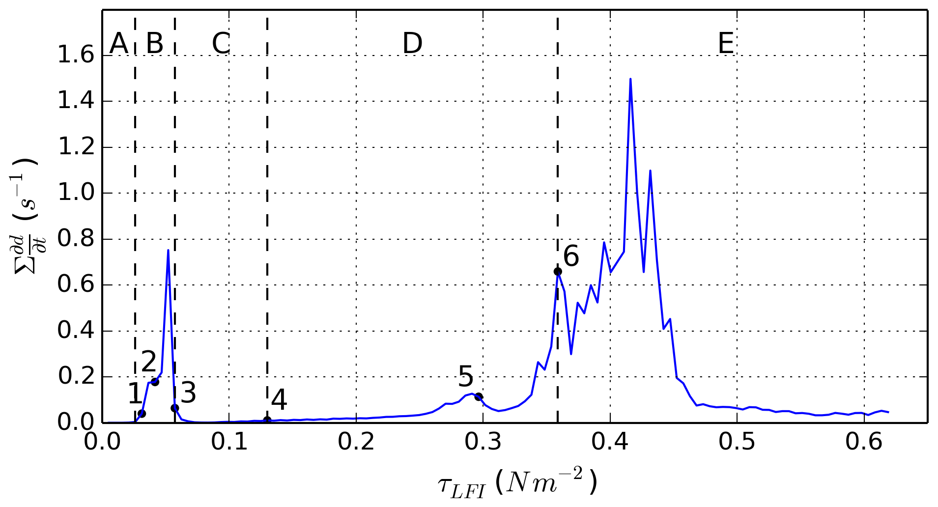
In the first stage of the simulation, elastic stress builds up but remains inside the yield curve in the entire domain, such that there is no brittle failure activity (Fig. 4, Stage A). The sea ice in the elastic regime behaves as an elastic plate and deformations are linearly related to the internal stresses. The elastic stresses are determined by the orientation of the surface forcing with respect to the coastlines: there are large tensile stresses on the downstream coastlines, compressive stresses on the upstream coastlines and shear stresses on the four corners of the channel (Fig. 7). At the vertical line of symmetry (away from channel openings, Fig. 7a, dashed blue line), the simulated stress field is in good agreement with the analytical solutions from a 1D version of the momentum equation, giving us confidence in the numerical implementation of the model (see Appendix B and Fig. 8). Upstream and downstream of the channel, both stress invariants are important, reaching a maximum in magnitude at the channel corners and decreasing to a local minimum at the center of the channel. In this configuration, the second principal stress alignment (Fig. 7c) is along the x direction downstream of the coastlines (where the ice is in uniaxial tension) and along the y direction upstream of the coastlines (where the ice is in uniaxial compression). In the downstream end of channel, the second principal stress alignment follows the shape of an arch, transitioning to a vertical alignment towards the upstream channel entrance.

3.1.1 Downstream ice arch

The formation of the downstream ice arch is initiated at a surface forcing of ∼0.02 N m⁻². The initial fractures are located at the downstream corners of the channel where the stress state reaches the critical shear strength for positive (tensile) normal stresses. The fractures then propagate from these locations and form an arch (see Fig. 5a). The progression of the fracture into an ice arch is helped by the concentration of stresses at the channel corners and around the subsequent damage. That is, the damage permanently decreases the elastic stiffness, which leads to locally larger elastic deformations and increases the load in the surrounding areas, leading to the propagation of the fractures in space through regions where the internal stress state was originally subcritical. In the first order, the arching progression of the fracture from the channel corners follows the second principal stress direction (i.e., a failure in uniaxial tension on the plane perpendicular to the maximum tensile stress; see Fig. 7c). This differs from the expected angle of fracture in a Coulombic material of $\mathit{\theta }=\pm (\mathit{\pi }/\mathrm{4}-\mathit{\varphi }/\mathrm{2})$ from the second principal stress orientation (Ringeisen et al., 2019), as reported in Dansereau et al. (2019).

Figure 5 (a) Damage field at the surface forcing indicated by points 1, 2 and 3 in Fig. 4 during the formation of the downstream ice arch. (b) Sea ice thickness and drift following the formation of the downstream ice arch, while the ice bridge remains stable (Phase C).

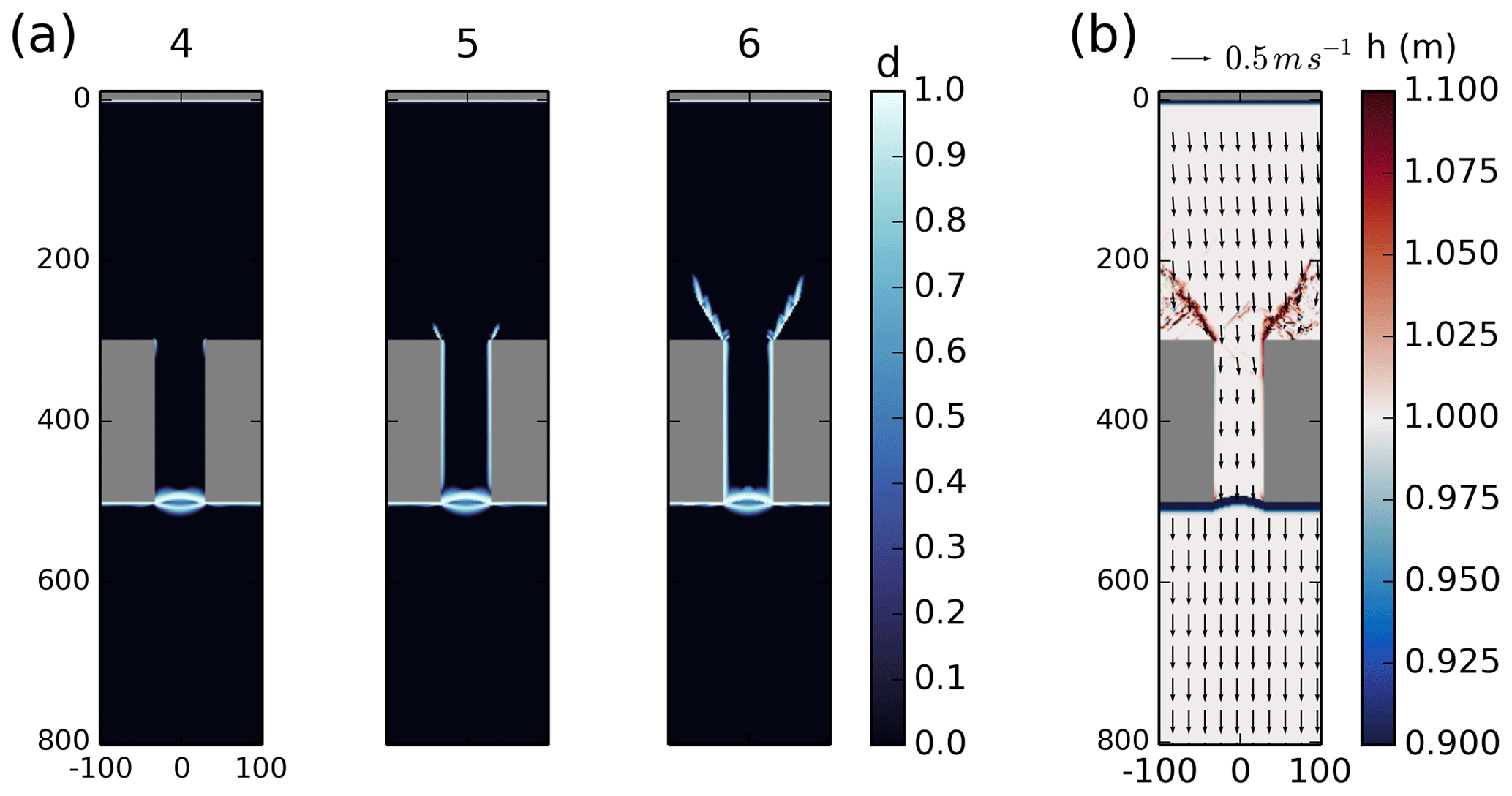
Figure 6 (a) Damage field at the surface forcing indicated by points 4, 5 and 6 in Fig. 4 during the formation of the upstream lines of fracture. (b) Sea ice thickness and drift following the ice bridge collapse (Phase E).

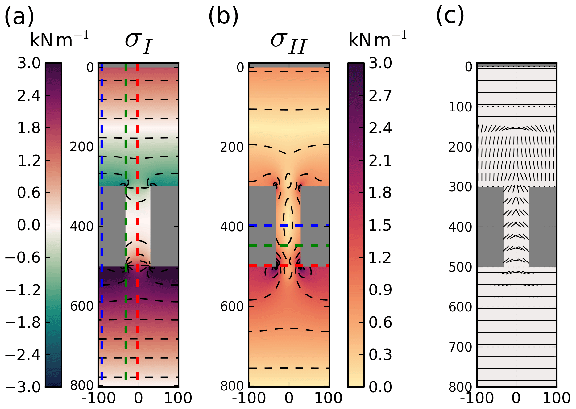
Figure 7 Stress fields in landfast ice during Phase A. (a) Normal stress invariant (σ_I) with colored dashed lines to indicate the vertical transects used in Fig. 8, (b) shear stress invariant (σ_II) with colored lines to indicate the horizontal transects used in Fig. 8 and the (c) orientation of the second principal stress component.

A second period of low brittle fracture activity follows the formation of the ice arch (period C in Fig. 4). In this stage, the ice downstream of the ice arch is detached from the land boundaries and starts to drift. The nonzero brittle fracture activity in this stage is due to the increased damage in regions of already damaged ice; since the local stress state lies on the yield curve, the increasing forcing constantly increases the stress states beyond the yield criterion, leading to further damage. Upstream of the ice arch, the elastic stresses show little change from Stage A, except for their increase in magnitude due to higher forcing (Fig. 9). As the yield parameters (c, σ_c) are not a function of the damage, tensile fracturing does not reduce the critical stress. This results in large tensile and shear stresses persisting along and north of the ice arch after its formation. The formation of a stress-free surface could be obtained by modifying the formulations of c and σ_c0 such that they depend on the damage.

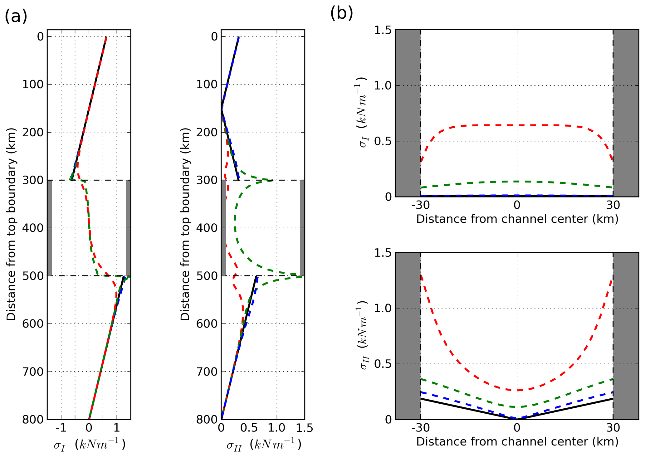
Figure 8 Stress invariants (σ_I, σ_II) along the transects of corresponding colors in Fig. 7: (a) transects running along the y direction and (b) transects running along the x direction. Solid black lines indicate the analytic solutions. The grey area indicates the position of the islands.

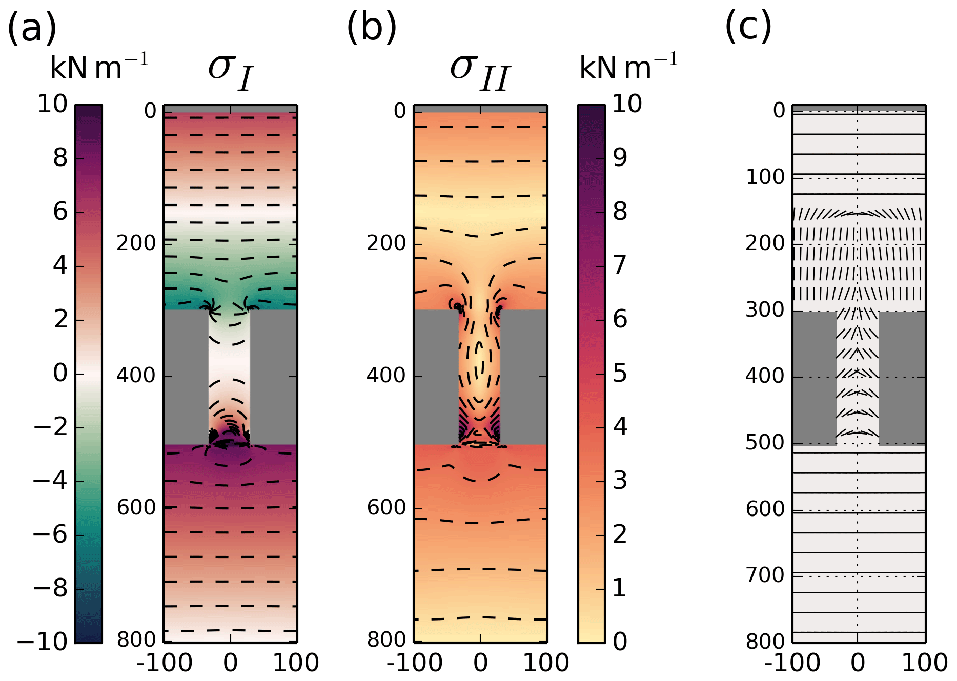
Figure 9 Stress fields during Phase C. (a) Normal stress invariant (σ_I), (b) shear stress invariant (σ_I) and (c) orientation of the second principal stress component.

3.1.2 Ice bridge collapse

The second break-up event (Stage D in Fig. 4) corresponds to the fracture of ice upstream of the channel and the collapse of the ice bridge. The fractures are initiated at a surface forcing of 0.13 N m⁻² on the upstream corners of the islands where the internal stress reaches the critical shear strength for negative (compressive) normal stresses. The propagation of damage from these locations is composed of two separate fractures (see Fig. 6a). First, a shear fracture progresses downstream along the channel walls, resulting in the decohesion of the landfast ice in the channel from the channel walls. The decohesion of the ice bridge increases the load on the downstream ice arch and on the landfast ice upstream of the channel. Second, a shear fracture propagates upstream from the channel corners at an angle 58^∘ from the coastline. The shear fracture orientation corresponds to an angle θ=32^∘ from the second principal stress orientation (Fig. 7c), which also deviates from the theoretical 22.5^∘ in a granular material with ϕ=45^∘ (Ringeisen et al., 2019).

Once the lines of fracture are completed, the ice bridge collapses and the ice in the channel starts to drift (Stage E). In this stage, landfast ice only remains in two wedges of undeformed ice upstream from the islands in which high compressive stress remains present (see Fig. 10a). The remaining continuous areas of undamaged ice drift downward into the funnel as a solid body with uniform velocity, with ridges building at the fracture lines. The ridge building is highly localized (see Fig. 6b) but slowly expands in the direction perpendicular to the lines of fracture. This follows from the increase in material strength with ice thickness, resulting in larger compressive stresses along the ridge such that the ice fracture occurs in the neighboring thinner ice, in a succession of fracture events that are localized in time (see peaks in Stage E in Fig. 4).

Figure 10 Stress fields during Phase E. (a) Normal stress invariant (σ_I), (b) shear stress invariant (σ_I) and (c) orientation of the second principal stress component.

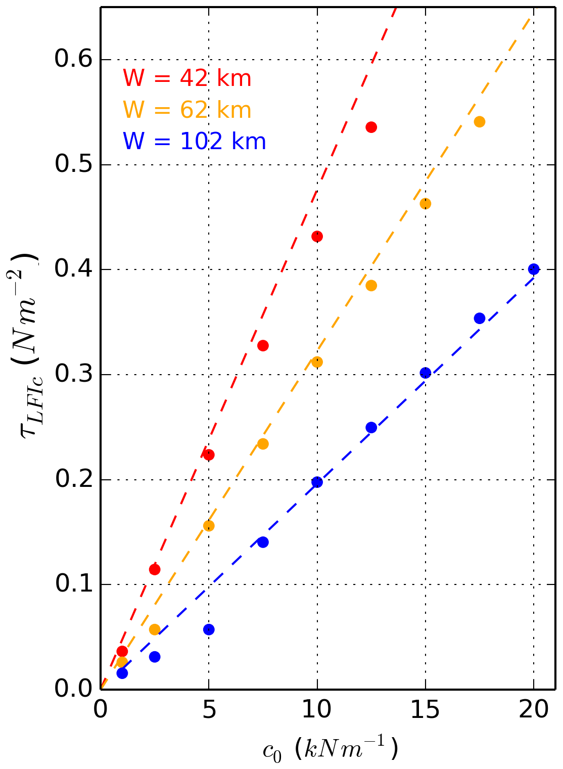
Figure 11 Critical surface forcing associated with the second fracture event (Stage D) as a function of cohesion and channel width (dots). Dashed lines indicate the analytic solution from the 1D equations.

3.2 Sensitivity to mechanical strength parameters

The Mohr–Coulomb yield criterion defines the shear strength of sea ice as a linear function of the normal stress on the fracture plane. In stress invariant coordinates (σ_I, σ_II), this can be written in terms of two material parameters: the cohesion c and the coefficient of internal friction μ=sin ϕ (Fig. 2). The isotropic tensile strength (i.e., the tip of the yield curve) is then a linear function of the two (${\mathit{\sigma }}_{\mathrm{t}}=c/\mathit{\mu }$). In this section, we investigate the influence of these material parameters and of the use of a uniaxial compressive strength criterion on the simulated ice bridge.

3.2.1 Cohesion

Changing only the cohesion c₀ (with a fixed internal angle of friction ϕ) moves the entire yield curve along the first stress invariant (σ_I) axis. For example, a higher cohesion increases the isotropic tensile strength ${\mathit{\sigma }}_{{\mathrm{t}}_{\mathrm{0}}}=c_{\mathrm{0}}/\sin \mathit{\varphi }$ and also increases the shear strength uniformly for all normal stress conditions. In the ice bridge simulations, the choice of cohesion influences the critical surface forcing associated with the different stages of the simulations but does not change the series of events described in Sect. 3.1 or the orientation of the ice fractures. This is in agreement with results from Dansereau et al. (2017).

The critical surface forcing associated with the ice bridge breakup can be related to the cohesion using the 1D steady-state momentum equation (see Appendix B for details). Assuming an infinite channel running in the y direction, the shear stress along the channel walls (σ_xy) is given by

$$\begin{array}{}\text{(39)}& \left|{\mathit{\sigma }}_{xy}\right|={\mathit{\sigma }}_{\mathrm{II}}={\displaystyle \frac{{\mathit{\tau }}_{\mathrm{LFI}}W}{\mathrm{2}}},\end{array}$$

where W is the channel width (see Fig. 3). Using the yield criterion (Eq. 10) with σ_I=0 (i.e., σ_II=c), the maximum sustainable surface forcing τ_LFIc can be related to the cohesion as follows:

$$\begin{array}{}\text{(40)}& {\mathit{\tau }}_{\mathrm{ac}}={\displaystyle \frac{\mathrm{2}c}{W}}.\end{array}$$

In the simulations, the critical forcing for the complete decohesion of ice bridges (point 5 in Figs. 4 and 6) with different widths follows the simple 1D model (Fig. 11). This indicates that although the fracture is initiated at a weaker forcing due to the concentration of stress at the channel corners, the ice arch sustains the increasing load such that the ice bridge remains stable.

Given that ice bridges and arches with a width of ∼60 km are frequent in the CAA (e.g., Nares Strait, Lancaster Sound or Prince Regent Inlet) and that the surface stresses regularly exceed 0.15 N m⁻² (e.g., corresponding to a wind speed of 10 m s⁻¹ or a tidal current of ∼0.15 m s⁻¹), this suggests a lower bound on the cohesion of sea ice of at least 5 kN m⁻¹ (see yellow curve in Fig. 11). Similarly, the fact that the ice bridges are rarely larger than 100 km (some are seen intermittently in the Kara Sea, Divine et al., 2004) indicates that the cohesion of sea ice should be smaller than 10 kN m⁻¹ (see red curve in Fig. 11). This range (5–10 kN m⁻¹) is lower than records from ice stress buoys measurements, which measure both thermal and mechanical internal stresses at smaller scales (40 kN m⁻², Weiss et al., 2007) but agree with estimates from ice arch observations (Sodhi, 1997). Note that higher forcing may be frequent in areas associated with strong tides, although these locations correspond to unstable landfast ice areas and recurrent polynyas (Hannah et al., 2009). Our estimates therefore provide a meaningful bound to be used in sea ice models.

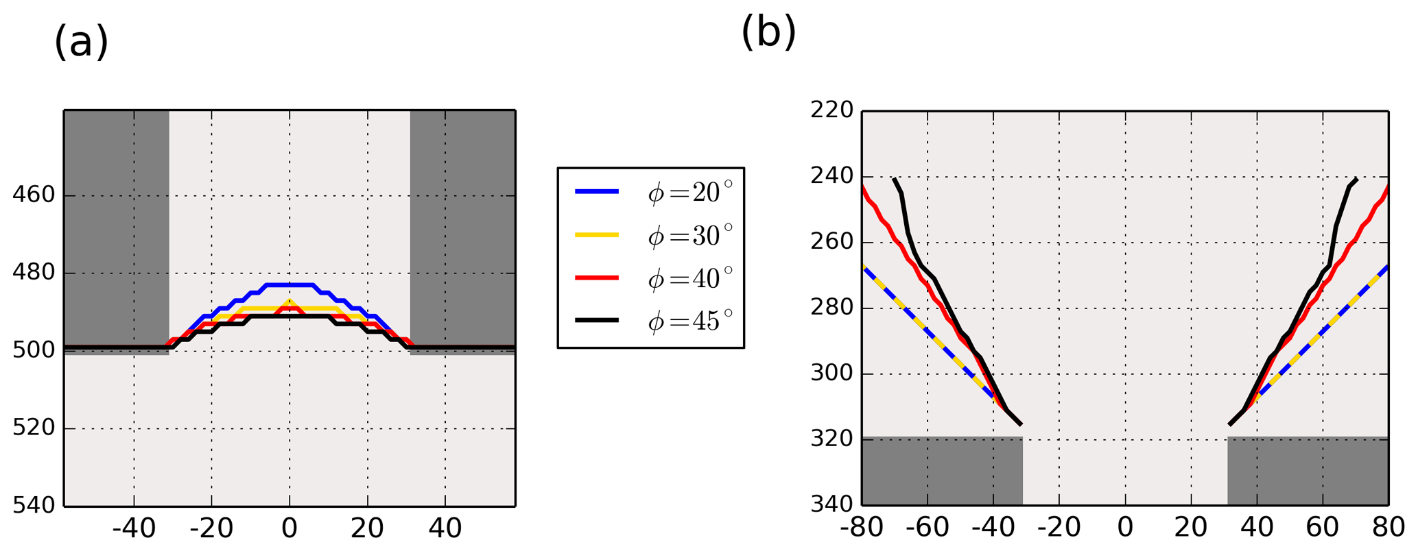
Figure 12 The shape of the lines of fracture using different angles of internal friction: (a) for the downstream ice arches and (b) for the upstream lines of fracture (the yellow and purple lines are superposed).

3.2.2 Angle of internal friction

The angle of internal friction ϕ, analogous to the static friction between two solids, determines the constant of proportionality between the shear strength and the normal stress (μ=sin ϕ; see Eq. 10 and Fig. 2). Varying the angle of internal friction changes the shear strength of ice under tensile and compressive stresses in opposite ways: when increasing the angle of internal friction, the shear strength of ice in tension is reduced while that of ice in compression is increased (and vice versa). This affects the critical forcing associated with the downstream and upstream ice fractures. When decreasing ϕ, the downstream ice arch (Stage B) forms under a stronger forcing, and a weaker forcing is required for the development of the upstream lines of fracture. As such, while the cohesion determines the stability of the landfast ice in the channel, the collapse of the ice bridge also requires the uniaxial fracture of ice upstream of the channel, which is sensitive to the angle of internal friction. The angle of internal friction also determines the shape of the ice fractures: decreasing ϕ leads to an increase in the curvature of the downstream ice arch and intensifies the departure of the upstream lines of fracture from the y axis (see Fig. 12). The simulated orientations of the fracture lines (32 and 45^∘ for ϕ=20 and 45^∘) differ from the orientations of 35 and 22.5^∘ predicted by the Mohr–Coulomb theory and do not vary linearly with the internal angle of friction.

3.2.3 Tensile strength

The yield curve modifications discussed above (varying c₀ and ϕ) also change the tensile strength (both uniaxial and isotropic) of ice. The tensile strength determines the magnitude of the critical surface forcing necessary for the formation of the downstream ice arch (Stage B). The tensile stresses downstream from the islands can be approximated using the 1D version of the momentum equation as a function of the fetch distance F_down (see Fig. 3) from the islands to the bottom boundary of the domain (derivation in Appendix B):

$$\begin{array}{}\text{(41)}& {\mathit{\sigma }}_{yy}={\mathit{\tau }}_{\mathrm{LFI}}{F}_{\mathrm{down}}.\end{array}$$

This can be written as a function of the material parameters using a simplified Mohr–Coulomb criterion (Eq. 10) for the 1D case (Appendix B):

$$\begin{array}{}\text{(42)}& {\mathit{\sigma }}_{\mathrm{II}}+\mathit{\mu }{\mathit{\sigma }}_{\mathrm{I}}={\displaystyle \frac{\mathrm{1}+\mathrm{2}\mathit{\mu }}{\mathrm{3}}}{\mathit{\sigma }}_{yy}<c,\end{array}$$

where $\mathit{\nu }=\mathrm{1}/\mathrm{3}$ was used. Substituting σ_yy from Eq. (41) into Eq. (42), the yield criterion can be written in terms of the surface forcing and the material parameters:

$$\begin{array}{}\text{(43)}& {\mathit{\tau }}_{\mathrm{LFI}}<{\displaystyle \frac{\mathrm{3}c}{F_{\mathrm{down}}(\mathrm{2}\mathit{\mu }+\mathrm{1})}}.\end{array}$$

Using our cohesion estimates ($\mathrm{5}<c<\mathrm{10}$ kN m⁻¹), angles of internal friction in the range of observations (30 and 45^∘) and a typical surface forcing of 0.15 N m⁻², this would suggest stable bands of landfast ice of extent F_down∼6–13 km to be sustainable. This is similar to observations in the Arctic, where bands of landfast ice rarely exceed tens of kilometers unless anchor points are provided by stamukhi (Mahoney et al., 2014).

3.2.4 Compressive strength criterion

While not used in other MEB implementations (Dansereau et al., 2016, 2017), the compressive cutoff offers a limit on the simulated uniaxial compression, which can reach unrealistically large values and cause numerical instabilities (see Sect. 4). Including a compressive strength criterion (${\mathit{\sigma }}_{\mathrm{I}}-{\mathit{\sigma }}_{\mathrm{II}}>{\mathit{\sigma }}_{\mathrm{c}}$) can modify the upstream fracture event (Stage D) via the development of uniaxial compression fractures along the upstream coast of the islands if the uniaxial compressive stress upstream of the islands exceeds the ice strength typically observed in the field (∼40 kN m⁻²; see Table 1). The critical surface forcing for the development of a compressive fracture can be approximated using the 1D version of the momentum equation. The maximum normal stress at the upstream coast of the islands is as follows:

$$\begin{array}{}\text{(44)}& {\mathit{\sigma }}_{yy}={\mathit{\tau }}_{\mathrm{LFI}}{F}_{\mathrm{up}},\end{array}$$

where F_up is the distance between the top boundary of the domain and the upstream coasts of the islands (see Fig. 3). In the ideal case, the compression strength criterion is as follows:

$$\begin{array}{}\text{(45)}& {\mathit{\sigma }}_{\mathrm{I}}-{\mathit{\sigma }}_{\mathrm{II}}=\mathit{\nu }{\mathit{\sigma }}_{yy}>{\mathit{\sigma }}_{\mathrm{c}}.\end{array}$$

The compression criterion can thus be written as a function of the surface forcing as follows:

$$\begin{array}{}\text{(46)}& {\mathit{\tau }}_{\mathrm{LFI}}>{\displaystyle \frac{{\mathit{\sigma }}_{\mathrm{c}}}{\mathit{\nu }{F}_{\mathrm{up}}}}.\end{array}$$

Whether the ice will fail in shear (Mohr–Coulomb criterion) or in compression can be evaluated by substituting τ_LFI from Eq. (39) into Eq. 46, yielding the following criterion:

$$\begin{array}{}\text{(47)}& {\displaystyle \frac{\mathrm{2}\mathit{\nu }{F}_{\mathrm{up}}c}{W}}>{\mathit{\sigma }}_{\mathrm{c}}.\end{array}$$

If this condition is met, the compression strength criterion does not influence the simulation, and the upstream shear fracture lines develop as in the control simulation (Fig. 13a). If the left-hand side of Eq. (47) is much smaller that σ_c, a compression fracture occurs before the ice bridge breakup and a ridge forms along the upstream coastlines, propagating in the channel entrance, while the ice in the channel remains landfast (Fig. 13b). If the terms are of a similar order, the decohesion of the ice bridge and the compression fractures are initiated simultaneously, such that the compression fracture occurs along the upstream coastlines but not in the channel entrance, as the ice starts to drift in and upstream of the channel (Fig. 13c).

Figure 13 Spatial distribution of the damage field at the end of Stage D (left panels) and the sea ice thickness and velocity fields at the end of the simulation (right panels) for different compressive strength criteria: (a) ${\mathit{\sigma }}_{c_{\mathrm{0}}}=\mathrm{100.0}$ kN m⁻¹, (b) ${\mathit{\sigma }}_{c_{\mathrm{0}}}=\mathrm{5.0}$ kN m⁻¹ and (c) ${\mathit{\sigma }}_{c_{\mathrm{0}}}=\mathrm{25.0}$ kN m⁻¹.

4 Discussion

In the Arctic, ice arches are commonly observed upstream of narrow channels, where granular floes jam when forced into the narrowing passage. This requires the ice to not to be landfast in the channel itself (Vincent, 2019), as opposed to the simulations presented above where the ice is initially landfast in the model domain. Contrary to results presented in Dansereau et al. (2017) where the presence of floes is simulated by a random seeding of weaknesses in the initial ice field, unstable ice arches upstream of the channel are not present in our simulations. Instead, our experiment simulates the propagation of ice fractures through the landfast ice upstream of a channel, which are akin to a failure in uniaxial compression (Dansereau et al., 2016; Ringeisen et al., 2019).

In theory, the angle of internal friction governs the intersection angle between lines of fracture (Marko and Thomson, 1977; Pritchard, 1988; Wang, 2007; Ringeisen et al., 2019). That is, the lines of fracture are oriented at an angle $\mathit{\theta }(=\mathit{\pi }/\mathrm{2}-\mathit{\varphi }/\mathrm{4}$) with the second principal stress direction, where the ratio of shear to normal stress is largest. In our simulations, the angles of fracture, although sensitive to the angle of internal friction, do not follow this theory. The fact that different angles of internal friction yield the same fracture orientation (e.g., for ϕ=20^∘ and ϕ=30^∘; see Fig. 12) indicates that the orientation is not directly associated to the yield criterion in the MEB rheology (there is no flow rule in the MEB rheology). However, the orientation of the lines of fracture do have a sensitivity to the angle of internal friction, which suggests that the deformations are at least indirectly influenced by the yield criterion. This is in accord with previous results showing that the fracture orientation is determined by the concentration of stress along lines damage instability (Dansereau et al., 2019). This raises the question whether the lines of fracture may be influenced by the stress correction path used in the damage parameterization, which determines the stress state associated with the fractures. These questions are left for future work and will be addressed using a simple uniaxial loading numerical experiments (e.g., Ringeisen et al., 2019).

We speculate that in a longer simulation, ice would eventually jam between the upstream lines of fracture, resulting in the formation of a stable ice arch upstream of the channel. This is suggested by the orientation of the second principal stress component upstream of the channel (Fig. 10c). Longer-term simulations, however, are prevented by the presence of numerical instabilities associated with the current damage parameterization. As the integration progresses, the simulated fields lose their longitudinal symmetry at about the center line of the domain. This loss of symmetry occurs more rapidly as the residual norm increases (Fig. 14) and is not due to a difficulty in solving the equations: the nonlinear solver converges rapidly, within six iterations, given the small time step required by the CFL criterion to resolve the elastic waves. The errors are instead related to the integration of the residual norms in the model memory terms in the constitutive equation. The integrated error is only dissipated over a large number of time steps, such that the error in the solution is orders of magnitude larger than the set residual norm tolerance. This limits the current analysis to short-term simulations in which this issue remains negligible.

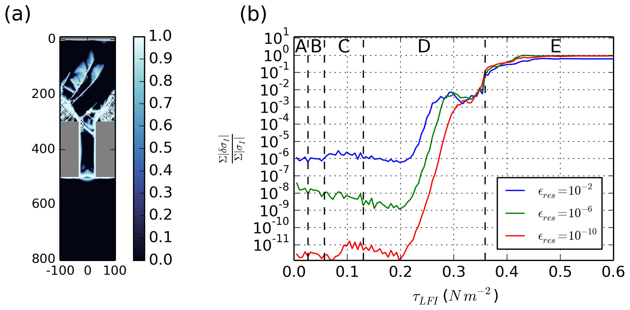
Figure 14 (a) Asymmetries dominating the damage fields after the ice bridge collapse (Stage E) in Fig. 4. (b) Evolution of normalized, domain-integrated asymmetries in the σ_I field when using different residual tolerance ϵ_res on the solution. Dashed lines indicate the beginning and end of the simulation phases (A, B, C, D, E).

An error propagation analysis shows that the instabilities are largely attributed to the stress correction scheme and the computation of the damage factor Ψ (Eq. 13). Assuming that the model is iterated to convergence such that the uncorrected stress state has a relative error ϵ, the error on the corrected stress is as follows (see derivation in Appendix C):

$$\begin{array}{}\text{(48)}& {\mathit{ϵ}}_{\mathrm{M}}=\mathit{ϵ}\sqrt{\mathrm{1}+R},\end{array}$$

where

$$\begin{array}{}\text{(49)}& R={\displaystyle \frac{{{\mathit{\sigma }}_{\mathrm{II}}^{\prime }}^{\mathrm{2}}+{\mathit{\mu }}^{\mathrm{2}}{{\mathit{\sigma }}_{\mathrm{I}}^{\prime }}^{\mathrm{2}}}{({\mathit{\sigma }}_{\mathrm{II}}^{\prime }+\mathit{\mu }{\mathit{\sigma }}_{\mathrm{I}}^{\prime }{)}^{\mathrm{2}}}}.\end{array}$$

If ${\mathit{\sigma }}_{\mathrm{I}}^{\prime }>\mathrm{0}$ (tensile stress state), $\mathrm{0}<R<\mathrm{1}$ (triangle inequality) and the error on the memory terms (ϵ_M) is of the same order as that of the uncorrected stress state ($\mathit{ϵ}\le {\mathit{ϵ}}_{\mathrm{M}}\le \sqrt{\mathrm{2}}\mathit{ϵ}$). If ${\mathit{\sigma }}_{\mathrm{I}}^{\prime }<\mathrm{0}$ (compressive stress state), we have R≥1, the error on the stress memory can become orders of magnitude larger than that of the uncorrected stress state, and the model accuracy and convergence properties are greatly reduced. These errors are stored in the memory terms and accumulate at each fracture event. Note that as the elastic stress memory is dissipated over the viscous relaxation timescale, and this issue could be mitigated by decreasing the viscous coefficients η₀. Using a compressive strength cutoff capping also offers a limit to the uniaxial compression and reduces this instability. Another solution could be using a nonlinear yield curve which converges to the Tresca criterion (σ_II=const) for large compressive stresses (e.g., the yield criterion of Schreyer et al., 2006). We, however, argue that this issue in the damage parameterization should be treated by bringing the stress back onto the yield curve along a different path (e.g., following a line perpendicular to the curve). It might also be possible to use a different stress correction path to constrain the orientation of the lines of fractures to the yield criterion. This will be assessed in future work.

5 Conclusions

The MEB rheology is implemented in the Eulerian FD numerical framework of the McGill sea ice model. We show that the discretized Maxwell stress–strain relationship can be written in a form that resembles that of the VP model, with an additional memory term. The MEB rheology is then simply implemented by redefining the VP viscous coefficients in terms of the MEB parameters and by adding the damage parameterization in a separate module. To our knowledge, it is the first time the MEB rheology has been implemented in the same framework as a VP or EVP model. This will allow direct comparison of these models using the same numerical platform in future work.

In idealized ice bridge simulations, we show that the damage parameterization allows the ice fractures in the MEB model to propagate over large distances at short timescales. This process relies on the memory of the past deformations included in the model, which causes a concentration of stresses close to the preexisting damage. We also show that while the choice of yield curve influences the localization and orientation of the ice fractures, the angles of fracture propagation differ from those expected from the Mohr–Coulomb theory. This is consistent with results from Dansereau et al. (2019) that show that the fracture orientation is determined by the planes of damage instability. Preliminary results suggest that the orientation of the fracture lines are influenced by the stress correction scheme. This will be the subject of future work.

The stress correction scheme in the damage parameterization (Rampal et al., 2016) is also found to cause a problematic increase in the numerical errors in the stress memory terms. The growth of errors depends on the magnitude of the compressive stress associated with the ice failure. These errors accumulate in the memory term at each fracture event, creating numerical artifacts that dominate the solutions over time. We argue that this weakness of the damage parameterization should be treated as a numerical issue. In previous MEB implementations, asymmetries are expected due to either the asymmetric coastlines and forcing (Rampal et al., 2016) or the material heterogeneity used to initialize the model (Dansereau et al., 2016), such that this instability difficult to detect. A possible solution to this problem would be to use a nonlinear yield curve that converges to the Tresca criterion for large compressive stresses (e.g., the yield criterion of Schreyer et al., 2006). It may also be possible to eliminate this numerical noise by using a different stress correction scheme that does not follow a path to the origin. This will be assessed in future work.

The simulated breakup of the landfast ice bridge occurs with two main fracture events. First, an ice arch develops at the downstream end of the channel, shaping the edge of the ice bridge in the channel. This ice arch forms in all simulations and is stable in shape as long as the ice bridge remains in place, with a curvature that increases for smaller angles of internal friction. Second, shear fractures are formed at the upstream end of the channel, resulting in the decohesion of the channel ice bridge and the formation of landfast wedges upstream of the islands. Based on the simulation results, we determined that the parameterized cohesion most consistent to the observed ice bridges in the Arctic is in the range of 5–10 kN m⁻², lower than stress buoys that measure both dynamical and thermal stresses at smaller scales but in the range of values previously associated to ice arch observations.

Appendix A: Damage factor Ψ

Let ${\mathit{\sigma }}_{\mathrm{I}}^{\prime }$ and ${\mathit{\sigma }}_{\mathrm{II}}^{\prime }$ be the stress invariant at time level n before the correction is applied and σ_If and σ_IIf be the corrected stress invariant lying on the yield curve. Following Bouillon and Rampal (2015), we use a damage factor Ψ ($\mathrm{0}<\mathrm{\Psi }<\mathrm{1}$) to reduce the elastic stiffness and bring the stress state onto the yield curve, i.e.,

$$\begin{array}{}\text{(A1)}& {\mathit{\sigma }}_{\mathrm{If}}=\mathrm{\Psi }{\mathit{\sigma }}_{\mathrm{I}}^{\prime };{\mathit{\sigma }}_{\mathrm{IIf}}=\mathrm{\Psi }{\mathit{\sigma }}_{\mathrm{II}}^{\prime }.\end{array}$$

Substituting these relations into the Mohr–Coulomb criterion (${\mathit{\sigma }}_{\mathrm{IIf}}+\mathit{\mu }{\mathit{\sigma }}_{\mathrm{If}}=c$), we solve for Ψ:

$$\begin{array}{}\text{(A2)}& \mathrm{\Psi }={\displaystyle \frac{c}{{\mathit{\sigma }}_{\mathrm{II}}^{\prime }+\mathit{\mu }{\mathit{\sigma }}_{\mathrm{I}}^{\prime }}}.\end{array}$$

Note that this relation implies that the stress correction is done following a line from the stress state (${\mathit{\sigma }}_{\mathrm{I}}^{\prime }$, ${\mathit{\sigma }}_{\mathrm{II}}^{\prime }$) to the origin (see Fig. 2). This scheme stems from applying the damage factor to each individual stress component. Other paths could be used for the correction (e.g., following a vertical or horizontal line) but would require the use of a different stress factor for the different components of the stress tensor. This could be used to cure the error propagation problem when large compressive stresses are present (see Appendix C).

Appendix B: Analytical solutions of the 1D momentum equation

Considering an infinite channel of landfast ice (u=0) along the y direction with forcing τ_LFY=τ_y, we write the 1D steady-state momentum equation as follows:

$$\begin{array}{}\text{(B1)}& {\displaystyle \frac{\partial {\mathit{\sigma }}_{xy}}{\partial x}}+{\mathit{\tau }}_y=\mathrm{0},\end{array}$$

where we have neglected the $\partial /\partial y$ terms. In this case, the normal stress is zero in the entire channel and the stress invariants are σ_I=0, σ_II=σ_xy. The shear stress at any arbitrary point x across the channel can be determined by integrating Eq. (B1) from the channel center (x=0) to x:

$$\begin{array}{}\text{(B2)}& {\mathit{\sigma }}_{xy}=-{\mathit{\tau }}_{y}x.\end{array}$$

By symmetry, the maximum shear stresses in the channel are located at the channel walls at $x=\pm \frac{W}{\mathrm{2}}$, where W is the width of the channel. The maximum shear stress invariant on the channel walls is then

$$\begin{array}{}\text{(B3)}& {\mathit{\sigma }}_{\mathrm{II}}={\displaystyle \frac{W{\mathit{\tau }}_y}{\mathrm{2}}}.\end{array}$$

Similarly, we find the analytical solution for the normal stresses in a band of landfast ice with width L_y along an infinite coastline running in the x direction with a surface forcing τ_LFI=τ_y, by integrating the 1D momentum equation in which the $\partial /\partial x$ terms are neglected, i.e.,

$$\begin{array}{}\text{(B4)}& {\displaystyle }& {\displaystyle \frac{\partial {\mathit{\sigma }}_{yy}}{\partial y}}+{\mathit{\tau }}_y=\mathrm{0},\text{(B5)}& {\displaystyle }& {\displaystyle }{\mathit{\sigma }}_{yy}=-{\mathit{\tau }}_{y}y.\end{array}$$

Placing the landfast ice edge (where σ_yy=0) at y=0, the largest compressive stresses will be located along the coast, at $y=-L_y$. Note that in this case, shear stress is zero in the entire landfast ice and the stress invariants are function of both σ_xx and σ_yy:

$$\begin{array}{}\text{(B6)}& {\displaystyle }& {\displaystyle }{\mathit{\sigma }}_{yy}=E{C}_{\mathrm{1}}{\mathit{ϵ}}_{yy},\text{(B7)}& {\displaystyle }& {\displaystyle }{\mathit{\sigma }}_{xx}=E{C}_{\mathrm{2}}{\mathit{ϵ}}_{yy}=\mathit{\nu }{\mathit{\sigma }}_{yy},\text{(B8)}& {\displaystyle }& {\displaystyle }{\mathit{\sigma }}_{\mathrm{I}}={\displaystyle \frac{{\mathit{\sigma }}_{xx}+{\mathit{\sigma }}_{yy}}{\mathrm{2}}}={\displaystyle \frac{(\mathrm{1}+\mathit{\nu }){\mathit{\sigma }}_{yy}}{\mathrm{2}}},\text{(B9)}& {\displaystyle }& {\displaystyle }{\mathit{\sigma }}_{\mathrm{II}}=\sqrt{({\displaystyle \frac{{\mathit{\sigma }}_{yy}-{\mathit{\sigma }}_{xx}}{\mathrm{2}}}{)}^{\mathrm{2}}}={\displaystyle \frac{(\mathrm{1}-\mathit{\nu }){\mathit{\sigma }}_{yy}}{\mathrm{2}}}.\end{array}$$

This allows us to write the Mohr–Coulomb criterion in terms of σ_yy:

$$\begin{array}{}\text{(B10)}& {\mathit{\sigma }}_{\mathrm{II}}+\sin \mathit{\varphi }{\mathit{\sigma }}_{\mathrm{I}}={\displaystyle \frac{\mathrm{1}+\mathrm{2}\sin \mathit{\varphi }}{\mathrm{3}}}{\mathit{\sigma }}_{yy}<c.\end{array}$$

Appendix C: Error propagation analysis

The error δF associated with a function $F(X,Y,Z,\mathrm{\dots })$ with uncertainties $(\mathit{\delta }x,\mathit{\delta }y,\mathit{\delta }z,\mathrm{\dots })$ is given by

$$\begin{array}{}\text{(C1)}& \mathit{\delta }F=\sqrt{({\displaystyle \frac{\partial F}{\partial X}}{)}^{\mathrm{2}}\mathit{\delta }{x}^{\mathrm{2}}+({\displaystyle \frac{\partial F}{\partial Y}}{)}^{\mathrm{2}}\mathit{\delta }{y}^{\mathrm{2}}+({\displaystyle \frac{\partial F}{\partial Z}}{)}^{\mathrm{2}}\mathit{\delta }{z}^{\mathrm{2}}+\mathrm{\dots }}.\end{array}$$

In the damage parameterization, the components of the corrected stress tensor used as the memory terms (σ_ijM) can be written in terms of the uncorrected stress tensor (${\mathit{\sigma }}_{ij}^{\prime }$) and the damage factor Ψ (Eq. 13):

$$\begin{array}{}\text{(C2)}& {\mathit{\sigma }}_{ij\mathrm{M}}=\mathrm{\Psi }{\mathit{\sigma }}_{ij}^{\prime }.\end{array}$$

Using Eq. (A2), this can be rewritten in terms of the uncorrected stress invariants (${\mathit{\sigma }}_{\mathrm{I}}^{\prime }$, ${\mathit{\sigma }}_{\mathrm{II}}^{\prime }$):

$$\begin{array}{}\text{(C3)}& {\mathit{\sigma }}_{ij\mathrm{M}}({\mathit{\sigma }}_{ij}^{\prime },{\mathit{\sigma }}_{\mathrm{I}}^{\prime },{\mathit{\sigma }}_{\mathrm{II}}^{\prime })={\displaystyle \frac{c{\mathit{\sigma }}_{ij}^{\prime }}{{\mathit{\sigma }}_{\mathrm{II}}^{\prime }+\mathit{\mu }{\mathit{\sigma }}_{\mathrm{I}}^{\prime }}}.\end{array}$$

Assuming that the model has converged to a solution within an error on the stresses $\mathit{\delta }{\mathit{\sigma }}_{ij}^{\prime }=\mathit{ϵ}{\mathit{\sigma }}_{ij}^{\prime }$, $\mathit{\delta }{\mathit{\sigma }}_{\mathrm{I}}^{\prime }=\mathit{ϵ}{\mathit{\sigma }}_{\mathrm{I}}^{\prime }$, $\mathit{\delta }{\mathit{\sigma }}_{\mathrm{II}}^{\prime }=\mathit{ϵ}{\mathit{\sigma }}_{\mathrm{II}}^{\prime }$, where ϵ is a small number, the model convergence error propagates on the stress memory with an error of

$$\begin{array}{}\text{(C4)}& \begin{array}{rl}& \mathit{\delta }{\mathit{\sigma }}_{ij\mathrm{M}}\\ & =\sqrt{({\displaystyle \frac{\partial {\mathit{\sigma }}_{ij\mathrm{M}}}{\partial {\mathit{\sigma }}_{ij}^{\prime }}}{)}^{\mathrm{2}}\mathit{\delta }{{\mathit{\sigma }}_{ij}^{\prime }}^{\mathrm{2}}+({\displaystyle \frac{\partial {\mathit{\sigma }}_{ij\mathrm{M}}}{\partial {\mathit{\sigma }}_{\mathrm{I}}^{\prime }}}{)}^{\mathrm{2}}\mathit{\delta }{{\mathit{\sigma }}_{\mathrm{I}}^{\prime }}^{\mathrm{2}}+({\displaystyle \frac{\partial {\mathit{\sigma }}_{ij\mathrm{M}}}{\partial {\mathit{\sigma }}_{\mathrm{II}}^{\prime }}}{)}^{\mathrm{2}}\mathit{\delta }{{\mathit{\sigma }}_{\mathrm{II}}^{\prime }}^{\mathrm{2}}}.\end{array}\end{array}$$

Substituting ($\mathit{\delta }{\mathit{\sigma }}_{ij}^{\prime }$, $\mathit{\delta }{\mathit{\sigma }}_{\mathrm{I}}^{\prime }$, $\mathit{\delta }{\mathit{\sigma }}_{\mathrm{II}}^{\prime }$) for ϵ and using Eq. (C3), we obtain

$$\begin{array}{}\text{(C5)}& \begin{array}{rl}\mathit{\delta }{\mathit{\sigma }}_{ij\mathrm{M}}& =\sqrt{{\displaystyle \frac{c^{\mathrm{2}}}{({\mathit{\sigma }}_{\mathrm{II}}^{\prime }+\mathit{\mu }{{\mathit{\sigma }}^{\mathbf{\prime }}}_{\mathrm{I}}{)}^{\mathrm{2}}}}{\mathit{ϵ}}^{\mathrm{2}}{{\mathit{\sigma }}_{ij}^{\prime }}^{\mathrm{2}}+{\displaystyle \frac{c^{\mathrm{2}}{{\mathit{\sigma }}^{\prime }}_{ij}^{\mathrm{2}}{\mathit{\mu }}^{\mathrm{2}}}{({{\mathit{\sigma }}^{\mathbf{\prime }}}_{\mathrm{II}}+\mathit{\mu }{\mathit{\sigma }}_{\mathrm{I}}^{\prime }{)}^{\mathrm{4}}}}{\mathit{ϵ}}^{\mathrm{2}}{{\mathit{\sigma }}_{\mathrm{I}}^{\prime }}^{\mathrm{2}}},\\ & \stackrel{\mathrm{‾}}{+{\displaystyle \frac{c^{\mathrm{2}}{{\mathit{\sigma }}^{\prime }}_{ij}^{\mathrm{2}}}{({{\mathit{\sigma }}^{\mathbf{\prime }}}_{\mathrm{II}}+\mathit{\mu }{{\mathit{\sigma }}^{\mathbf{\prime }}}_{\mathrm{I}}{)}^{\mathrm{4}}}}{\mathit{ϵ}}^{\mathrm{2}}{{\mathit{\sigma }}_{\mathrm{II}}^{\prime }}^{\mathrm{2}}}\end{array},\end{array}$$

or

$$\begin{array}{}\text{(C6)}& \mathit{\delta }{\mathit{\sigma }}_{ij\mathrm{M}}=\mathit{ϵ}{\mathit{\sigma }}_{ij\mathrm{M}}\sqrt{\mathrm{1}+{\displaystyle \frac{{{\mathit{\sigma }}_{\mathrm{II}}^{\prime }}^{\mathrm{2}}+{\mathit{\mu }}^{\mathrm{2}}{{\mathit{\sigma }}_{\mathrm{I}}^{\prime }}^{\mathrm{2}}}{({\mathit{\sigma }}_{\mathrm{II}}^{\prime }+\mathit{\mu }{\mathit{\sigma }}_{\mathrm{I}}^{\prime }{)}^{\mathrm{2}}}}}.\end{array}$$

Assuming that the error on the stress memory components (ϵ_M) has the form δσ_ijM=ϵ_Mσ_ijM, we can express the relative error of the stress memory components as a function of the stress invariants as follows:

$$\begin{array}{}\text{(C7)}& {\mathit{ϵ}}_{\mathrm{M}}=\mathit{ϵ}\sqrt{\mathrm{1}+R},\end{array}$$

where

$$\begin{array}{}\text{(C8)}& R={\displaystyle \frac{{{\mathit{\sigma }}_{\mathrm{II}}^{\prime }}^{\mathrm{2}}+{\mathit{\mu }}^{\mathrm{2}}{{\mathit{\sigma }}_{\mathrm{I}}^{\prime }}^{\mathrm{2}}}{({\mathit{\sigma }}_{\mathrm{II}}^{\prime }+\mathit{\mu }{\mathit{\sigma }}_{\mathrm{I}}^{\prime }{)}^{\mathrm{2}}}}.\end{array}$$