Spectral attenuation of ocean waves in pack ice and its application in calibrating viscoelastic wave-in-ice models

We investigate a case of ocean waves through a pack ice cover captured by Sentinel-1A synthetic aperture radar (SAR) on 12 October 2015 in the Beaufort Sea. The study domain is 400 km by 300 km, adjacent to a marginal ice zone (MIZ). The wave spectra in this domain were reported in a previous study (Stopa et al., 2018b). In that study, the authors divided the domain into two regions delineated by the first appearance of leads (FAL) and reported a clear change of wave attenuation of the total energy between the two regions. In the present study, we use the same dataset to study the spectral attenuation in the domain. According to the quality of SAR-retrieved wave spectrum, we focus on a range of wave numbers corresponding to 9–15 s waves from the open-water dispersion relation. We first determine the apparent attenuation rates of each wave number by pairing the wave spectra from different locations. These attenuation rates slightly increase with increasing wave number before the FAL and become lower and more uniform against wave number in thicker ice after the FAL. The spectral attenuation due to the ice effect is then extracted from the measured apparent attenuation and used to calibrate two viscoelastic wave-in-ice models. For the Wang and Shen (2010b) model, the calibrated equivalent shear modulus and viscosity of the pack ice are roughly 1 order of magnitude greater than that in grease and pancake ice reported in Cheng et al. (2017). These parameters obtained for the extended Fox and Squire model are much greater, as found in Mosig et al. (2015) using data from the Antarctic MIZ. This study shows a promising way of using remote-sensing data with large spatial coverage to conduct model calibration for various types of ice cover.

Highlights. Three key points:

1. The spatial distribution of wave number and spectral attenuation in pack ice are analyzed from SAR-retrieved surface wave spectra.

2. The spectral attenuation rate of 9–15 s waves varies around 10⁻⁵ m² s⁻¹, with lower values in thicker semicontinuous ice fields with leads.

3. The calibrated viscoelastic parameters are greater than those found in pancake ice.

1 Introduction

Rapid reduction in Arctic ice in recent decades has become a focal point in climate change discussions (Comiso et al., 2008; Meier, 2017; Rosenblum and Eisenman, 2017; Stroeve and Notz, 2018). The reduction emphasizes the need to better understand the complex interaction between the sea ice, the ocean and the atmosphere. One of these interaction processes is between ocean waves and sea ice. Ocean waves help to shape the formation of new ice covers (Lange et al., 1989; Shen et al., 2001), break existing ice covers (Kohout et al., 2016), modify upper-ocean mixing (Smith et al., 2018) and potentially compress sea ice through wave radiation stress (Stopa et al., 2018a). In turn, ice covers suppress wave–wind interaction by reducing the fetch. They also alter wave dispersion and attenuation through scattering and dissipation (Squire, 2007, 2018, 2020).

Modeling surface gravity waves in polar oceans requires the knowledge of many source terms. These source terms include wind inputs and dissipation, nonlinear transfer between frequencies, and wave–ice interaction. WAVEWATCH III^® (WW3; WAVEWATCH III^® Development Group, 2019), one of the most widely used third-generation wind–wave models for global and regional wave forecasts, has implemented several dispersion and dissipation (IC0, IC1, IC2, IC3, IC4 and IC5) as well as scattering (IS1 and IS2) parameterizations, called “switches” in WW3, to estimate the effect of ice on waves. Of the two scattering switches, IS1 redistributes a constant fraction of the incoming wave energy to all directions isotropically. IS2 adopts a linear Boltzmann equation and an estimation of maximum floe diameter due to ice breakup to model wave scattering combined with a creep-related dissipation. As is discussed in Sect. 3.2, scattering is negligible in the present dataset; hence it will not be considered in the present study. Of the six different dispersion and dissipation parameterizations, IC0 and IC1 are out-of-date. IC4 is empirically determined from data obtained in the Southern Ocean. IC2 is based on a theory that states that wave damping is entirely due to the eddy viscosity in the water body beneath the ice cover. The other two parameterization, IC3 and IC5, both assume that wave damping is due to the processes within the ice cover alone. In this study, we will focus on IC3 and IC5 parameterizations. The same method may be applied to calibrate IC2. Both IC3 and IC5 theorize that sea ice can store and dissipate mechanical energy; hence they model the ice cover as a viscoelastic material. The storage property is reflected in the potential and elastic energy, and the dissipative property is in the equivalent viscous damping. The difference between IC3 and IC5 is that IC3 is an extension of the viscous ice layer model with a finite thickness (Keller, 1998) by including elasticity into a complex viscosity (Wang and Shen, 2010b), while IC5 is an extension of the thin elastic plate model (Fox and Squire, 1994) introduced by Mosig et al. (2015) by adding viscosity into a complex shear modulus (equivalent to the complex viscosity via the Voigt model). Below we refer to these two viscoelastic models as WS and FS, respectively. Each of the two models shows a frequency-dependent wave propagation determined by the dispersion relation. This relation, which depends on the viscoelastic parameters, specifies how the wave number $k=k_{\mathrm{r}}+i{k}_{\mathrm{i}}$ is related to the wave frequency f. The complex wave number k contains a real part k_r, which determines the wave speed, and an imaginary part k_i, which determines the damping rate. To use these models for wave forecasts in ice-covered seas, one needs to determine the viscoelastic parameters for all types of ice covers. To derive these parameters using first principles is challenging, as demonstrated by De Carolis et al. (2005), who obtained the viscosity of grease ice using principles in fluid mechanics of a suspension. Alternatively, an inverse method has been adopted to parameterize IC3. Using in situ data from the R/V Sikuliaq field experiment (Thomson et al., 2018), the WS model was calibrated to match the observed wave number and attenuation (Cheng et al., 2017). This calibration was carried out in a marginal ice zone (MIZ) populated predominantly with grease and pancake ice. Although it showed good agreement between the calibrated model and the field data in the frequency band containing most of the wave energy, these calibrated values are limited to the grease and pancake ice types. Further into the ice cover, where more rigid ice with larger floes is present, how the viscoelastic parameters might change is unknown at present. Note that models can only be as robust as the training data. Therefore, using a broader type of sea ice data will result in a more robust model.

Advancements made in remote-sensing technology have provided opportunities for such model calibration. Ardhuin et al. (2017) developed a method to conditionally invert from ice-covered water wave orbital motion to directional wave spectra from synthetic aperture radar (SAR) images based on the velocity-bunching mechanism. The methodology is further improved in Ardhuin et al. (2018) and Stopa et al. (2018b) to study wave state in the ice-covered Beaufort Sea using SAR images, which were captured during the R/V Sikuliaq field experiment by the satellite Sentinel-1A. Stopa et al. (2018b) retrieved wave-number-dependent spectra under the partially and fully ice-covered regions by substantially reducing data contamination by ice features with a similar-length scale as the wavelength. Using the SAR-retrieved wave spectra, Stopa et al. (2018b) found that the significant wave height attenuated steeply prior to the first appearance of ice leads (denoted as FAL hereafter), with a milder attenuation rate after the FAL. The definition of FAL is described in Appendix A. Furthermore, Monteban et al. (2019) used two overlapping burst images from the Sentinel-1 separated by ∼2 s to investigate wave dispersion in the Barents Sea. Based on the method proposed by Johnsen and Collard (2009), this time separation between subsequent images was sufficient to result in a less noisy and higher-quality imaginary spectrum, therefore allowing them to obtain spatiotemporal information of the dispersion relation. Their results showed that for long waves (100–350 m) in thin ice (<40 cm), the dispersion relation was the same as in open water.

This study uses the dataset reported in Stopa et al. (2018b). It includes two parts of data analysis: obtaining spectral wave attenuation rates from the retrieved wave data and then using these attenuation rates for wave-in-ice model calibration. This paper is organized as follows: Sect. 2 introduces the wave spectra data from Stopa et al. (2018b) used in this study. From this data, we obtain the dominant wave numbers and the related wave directions over the studied domain. In Sect. 3, we use the directional wave spectra to derive the apparent attenuation rate and then the attenuation rate due to sea ice alone. In Sect. 4, we calibrate two viscoelastic wave-in-ice models using the obtained wave-number-dependent attenuation data. The methodology presented in these two sections is similar to that in Cheng et al. (2017) with modifications to resolve the difference of the spectral data types of the waves. In Cheng et al. (2017), the spectral data were between energy and frequency, while in Stopa et al. (2018b) they were between energy and wave number. Section 5 discusses the characteristics of wavelength and attenuation in pack ice, calibrated viscoelastic parameters and wave attenuation modeling. The final conclusions are given in Sect. 6.

2 Data description

During the R/V Sikuliaq experiment, the Sentinel-1A, equipped with a synthetic aperture radar (SAR), acquired six sequential images around 16:50 UTC on 12 October 2015. These SAR images covered a 400 km by 1100 km region including open water, grease and pancake ice and pack ice (refer to Fig. 1 in Stopa et al., 2018b). A large wave event during this time with wave heights exceeding 4 m in the captured region provided quality wave data. From these SAR images, for most of this ice-covered region Stopa et al. (2018b) obtained two-dimensional wave spectra data E(k_x, k_y), where E indicates wave energy density and k_x and k_y are the wave number components in the range and azimuth directions of the satellite track, respectively. Details of this dataset and its retrieval may be found in Stopa et al. (2018b). We convert the two-dimensional spectrum at each location into an equivalent wave-number-direction spectrum E(k_r,θ), where $k_{\mathrm{r}}=\sqrt{k_x^{\mathrm{2}}+k_y^{\mathrm{2}}}$ and $\mathit{\theta }=\mathrm{atan}\left(k_y/k_x\right)$ indicate wave number and direction, respectively. The wave number is discretized from 0.011 to 0.045 m⁻¹ with an increment of 0.002 m⁻¹, and the direction is discretized into 360 bins with a 1^∘ bin width. We then define wave-number-dependent main wave directions for each given spectrum E(k_r,θ) in the following way: for each wave number k_r we fit the corresponding E curve with a Gaussian function (an example is given in Fig. S1 in the Supplement). The mean of this Gaussian function is defined as the main wave direction ${\mathit{\theta }}_{k_{\mathrm{r}}}$ for this k_r. Furthermore, we define the dominant wave number k_r,dominant to be the one corresponding to the maximum directionally integrated wave energy $\int E\left(k_{\mathrm{r}},\mathit{\theta }\right)\mathrm{d}\mathit{\theta }$.

An overview of the processed wave conditions in terms of the dominant wave number and its main direction is given in Fig. 1a along with the locations of the ice edge and other in situ observations. The associated ice conditions in the region are presented in Fig. 1b, c. Significant spatial variability is observed in both the wave and ice conditions. Figure 1a presents a subregion captured by the SAR images covering a portion of Alaska to the last azimuth position where waves are detectable in the images. Colors indicate the dominant wave number distribution of the retrievals, and arrows indicate their main directions. Cell size is coarsened to 12.5 km×12.5 km to enhance visualization. The ice edge is indicated by the contours of ice concentration (<0.4) from AMSR2 (Advanced Microwave Scanning Radiometer 2; https://seaice.uni-bremen.de/data/amsr2, last access: 21 June 2020, Spreen et al., 2008). An in situ buoy, AWAC-I (a subsurface Nortek acoustic wave and current buoy, moored at 150^∘ W, 75^∘ N), is marked by a magenta asterisk. Except for the in situ observations from the Sikuliaq ship (green diamond) and several drifting buoys (blue dots) near the ice edge, ice morphology information including ice types and their partial concentrations is absent. Nevertheless, the FAL (red dots) presumably marks the separation between discrete floes and a semicontinuous ice cover with dispersed leads. The ice condition below (before) the FAL was more complex, with thinner ice and lower concentration than that above (after) the FAL.

We select the study domain defined by the azimuth from 450 to 750 km and the range from 0 to 400 km. This domain contains most of the wave data retrieved in the pack ice field. Figure 1b, c show the distributions of ice concentration from AMSR2 and ice thickness from SMOS (Soil Moisture and Ocean Salinity; https://seaice.uni-bremen.de/data/smos, last access: 21 June 2020, Huntemann et al., 2014), respectively, in the region of interest. As shown in Cheng et al. (2017; Supplement Figs. S6 and S7), these two ice products compared the best with in situ observations in the MIZ. Their accuracies in the pack ice zone are uncertain. The purpose of this work is to retrieve the spectral wave attenuation and use the result to calibrate viscoelastic models in regions dominated by thin pack ice (thickness: <0.3 m). As shown in Fig. 1a, k_r,dominant generally declines crossing the FAL towards the north. Before the FAL, k_r,dominant increases in the direction of increasing range and decreasing ice concentration but is insensitive to ice thickness variation. After the FAL, k_r,dominant decreases in the wave-propagating direction (arrows) associated with the increase in ice thickness, where the ice field is presumably a semicontinuous cover populated with leads.

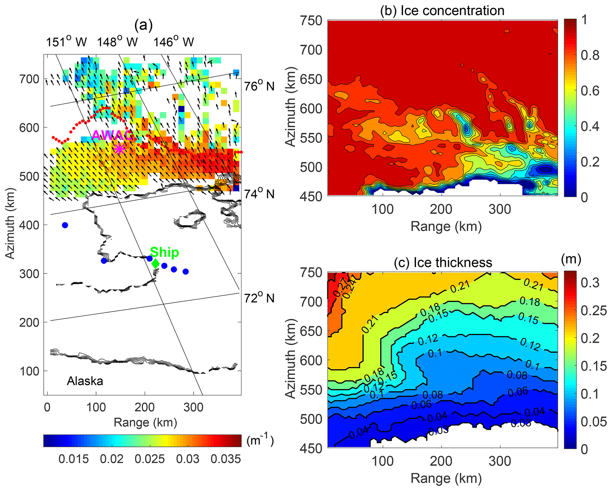
Figure 1 (a) Overview of the retrieved data distribution around 16:50 UTC on 12 October 2015. Colors represent the dominant wave number, and arrows represent the main direction of the dominant wave number. Red dots indicate the first appearance of leads (FAL). Locations of the Sikuliaq ship and the buoys operating at that time are indicated by a green diamond and blue dots, respectively. AWAC-I is marked by a magenta asterisk. Ice edges are indicated by contours of ice concentration <0.4 from AMSR2. (b, c) Distributions of ice concentration (AMSR2) and ice thickness (SMOS) in the selected region, respectively.

Figure 2a, b show two-dimensional histograms of the main wave direction for each wave number ${\mathit{\theta }}_{k_{\mathrm{r}}}$ before and after the FAL, respectively, where wave direction is defined in the meteorological convention (i.e., the direction “from” in degrees clockwise from true north). The gray scale indicates the occurrence frequency of ${\mathit{\theta }}_{k_{\mathrm{r}}}$ in each k_r bin. We observe a significant change in ${\mathit{\theta }}_{k_{\mathrm{r}}}$ crossing the FAL: before the FAL ${\mathit{\theta }}_{k_{\mathrm{r}}}$ spreads from 160 to 190^∘, while ${\mathit{\theta }}_{k_{\mathrm{r}}}$ is more tightly clustered from 180 to 200^∘ after the FAL. The difference before and after the FAL is most significant for k_r<0.035 m⁻¹.

For the subsequent spectral analysis, we further restrict k_r to 0.019 m${}^{-\mathrm{1}}\le k_{\mathrm{r}}\le min\left(\mathrm{2}\mathit{\pi }/{\mathit{\lambda }}_{\mathrm{c}},\mathrm{0.045}{\mathrm{m}}^{-\mathrm{1}}\right)$, where λ_c is the azimuth cutoff indicating the minimum resolvable wavelength from the SAR imagery (Stopa et al., 2015; Ardhuin et al., 2017). Below this wavelength, the patterns of ice-covered ocean surface roughness from SAR imagery are more related to ice features rather than waves (Stopa et al., 2018b). For k_r<0.019 m⁻¹, energy density $E\left(k_{\mathrm{r}},{\mathit{\theta }}_{k_{\mathrm{r}}}\right)$ is small with high spatial variation (Fig. B1 in Appendix B) and hence treated as a noise band and removed from further study.

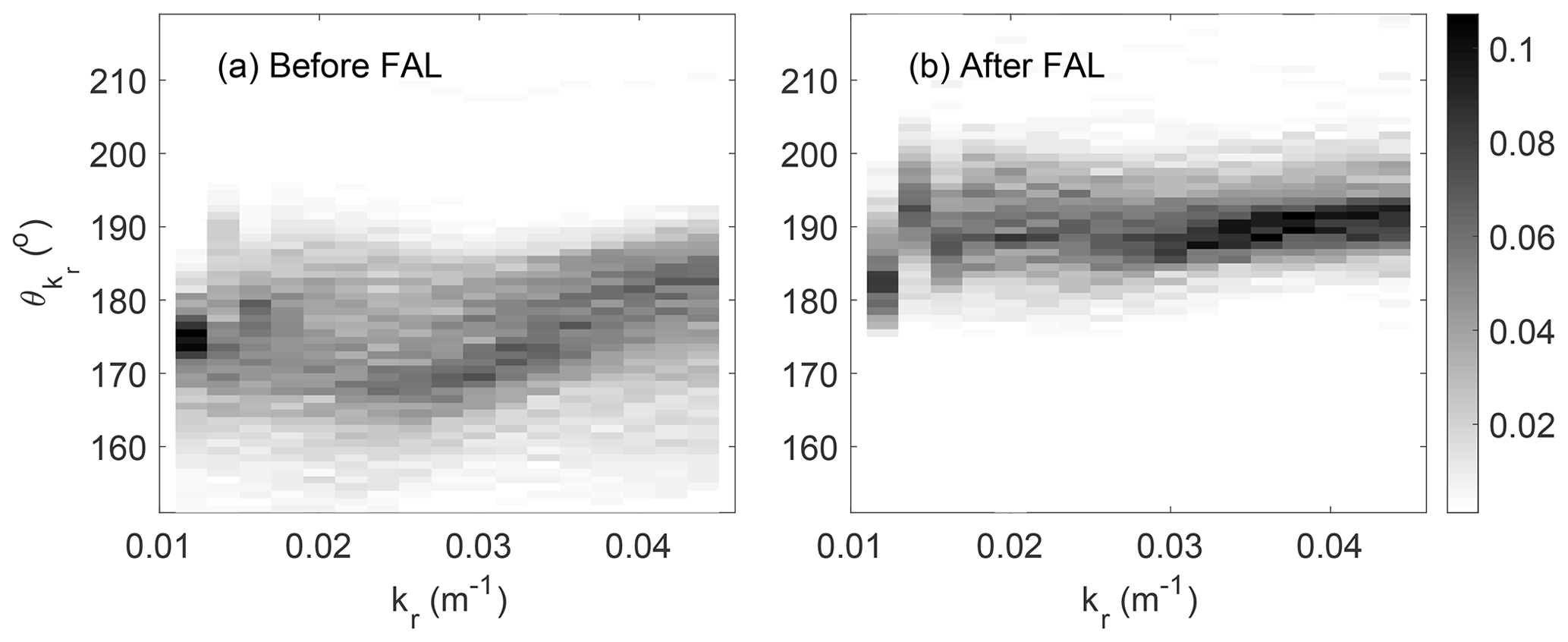
Figure 2 Two-dimensional histogram of ${\mathit{\theta }}_{k_{\mathrm{r}}}$ and k_r collected (a) before and (b) after the FAL. The gray scale represents the occurrence frequency of ${\mathit{\theta }}_{k_{\mathrm{r}}}$ in each k_r bin.

The corresponding frequency f (wave period T) range is estimated as 0.067 to 0.11 Hz (9 to 15 s) using the open-water dispersion relation (2πf)²=gk_ow, where g is the gravitational acceleration, and k_ow indicates the wave number in open water. The actual dispersion relation, which is likely dependent on the ice condition, cannot be measured from our instantaneous SAR data. Using accelerometers deployed on ice floes (Fox and Haskell, 2001) and from marine radar or buoy data (Collins et al., 2018), it was found that the wave number in the ice-covered region within about 10 km from the ice edge was close to that in open water. Further into the ice cover, Monteban et al. (2019) used two overlapping burst images from the Sentinel-1 separated by ∼2 s to investigate wave dispersion in the Barents Sea. The ice concentration and thickness in their study were similar to the present study. The computed wave dispersion within the sea ice for long waves (peak wavelengths: >100 m) was in good agreement with the open-water dispersion relation.

3 Wave attenuation

In this section, we first obtain the apparent spectral wave attenuation by pairing the directional spectra at different locations. We then remove the contributions of wave energy between pairs of locations from wind input, wave breaking dissipation and nonlinear transfer between frequency components to extract the spectral attenuation due to ice effects alone. These spectral attenuation rates due to ice are be used in Sect. 4 to calibrate two viscoelastic wave-in-ice models.

3.1 Apparent wave attenuation

We define an apparent wave attenuation for each k_r by assuming exponential decay of the wave spectral densities from location A to location B:

$$\begin{array}{}\text{(1)}& \mathit{\alpha }\left(k_{\mathrm{r}}\right)={\displaystyle \frac{\mathrm{1}}{\mathrm{2}D\cos \left(\left|\overline{\mathit{\theta }}-{\mathit{\theta }}_{AB}\right|\right)}}\ln \left({\displaystyle \frac{E_A\left(k_{\mathrm{r}},\overline{\mathit{\theta }}\right)}{E_B\left(k_{\mathrm{r}},\overline{\mathit{\theta }}\right)}}\right),\end{array}$$

where $\overline{\mathit{\theta }}=\frac{{\mathit{\theta }}_{k_{\mathrm{r},A}}+{\mathit{\theta }}_{k_{\mathrm{r},B}}}{\mathrm{2}}$ is the average of the main wave directions at A and B; D and θ_AB are the distance and direction from A to B in the longitude–latitude coordinates, respectively. A selected pair of A and B is named as a pair hereafter. To reduce the uncertainties of naturally present ice and wave variability, a set of quality control criteria are applied to a pair before further analysis:

1. Ignore substantially oblique waves. The difference between $\overline{\mathit{\theta }}$ and the vector from location A to location B is restricted to $\left|\overline{\mathit{\theta }}-{\mathit{\theta }}_{AB}\right|\le$15^∘.

2. Avoid strong spatial variations of ice condition between A and B. Distance between A and B is restricted to D≤60 km.

3. As the wave state changes significantly across the FAL as mentioned in Sect. 2, no pair across the FAL is selected. This criterion enables us to detect, if available, the influence of ice morphology on wave attenuation.

4. Ensure points A and B are both subject to the same wave system. The Pearson correlation coefficient between energy spectra E_A(k_r,θ) and E_B(k_r,θ) is required to be greater than 0.9. The Pearson correlation coefficient is defined as $r=\frac{{\mathrm{\Sigma }}_i\left(x_i-\overline{x}\right)\left(y_i-\overline{y}\right)}{\sqrt{{\mathrm{\Sigma }}_i{\left(x_i-\overline{x}\right)}^{\mathrm{2}}}\sqrt{{\mathrm{\Sigma }}_i{\left(y_i-\overline{y}\right)}^{\mathrm{2}}}}$, where x_i and y_i are the power spectral density (PSD) values at the ith wave number.

5. Exclude outliers of the spectral attenuation where the wave energy of B is higher or close to that of A. Thus, $\mathit{\alpha }\left(k_{\mathrm{r}}\right)>{\mathrm{10}}^{-\mathrm{6}}$ m⁻¹ is required.

6. A selected pair has to have at least 10 data points of α(k_r) to do calibration in Sect. 4.

We obtain 2634 pairs (2194 pairs before the FAL and 440 pairs after the FAL) through the above criteria to calculate the apparent wave attenuation α(k_r) by Eq. (1). The results are sorted statistically to show the occurrence frequency of α(k_r). The α domain is equally divided into 30 bins, from 10⁻⁶ to 10⁻⁴ m⁻¹ in log scale, and the k_r domain is equally divided from 0.011 to 0.045 m⁻¹ with an increment of 0.002 m⁻¹ as mentioned earlier. Figure 3a, b show two-dimensional histograms of α against k_r before and after the FAL, respectively. Gray scales represent the occurrence of α at each combined bin of α and k_r. Red curves indicate the most frequent occurrence of α(k_r) against k_r. It is observed that more data are obtained before the FAL, with a slightly increasing trend of α(k_r) versus k_r before the FAL, while α(k_r) obtained after the FAL are mostly lower and independent of k_r.

The range of this apparent spectral attenuation is in agreement with Stopa et al. (2018b), in which the authors selected multiple tracks throughout the ice region and focused on the overall decay of the significant wave height over hundreds of kilometers. The reduction in attenuation crossing the FAL shown in Fig. 3 is also consistent with Stopa et al. (2018b), who reported a drop in attenuation of the significant wave height after the FAL. In Appendix B, we show the results of this long-range attenuation against wave number (Fig. B1). The difference of attenuation obtained by the two methods, one based on short distances (<60 km) to reduce the effect of ice type variability and the other over long distances (∼300 km), is discussed in Sect. 5.

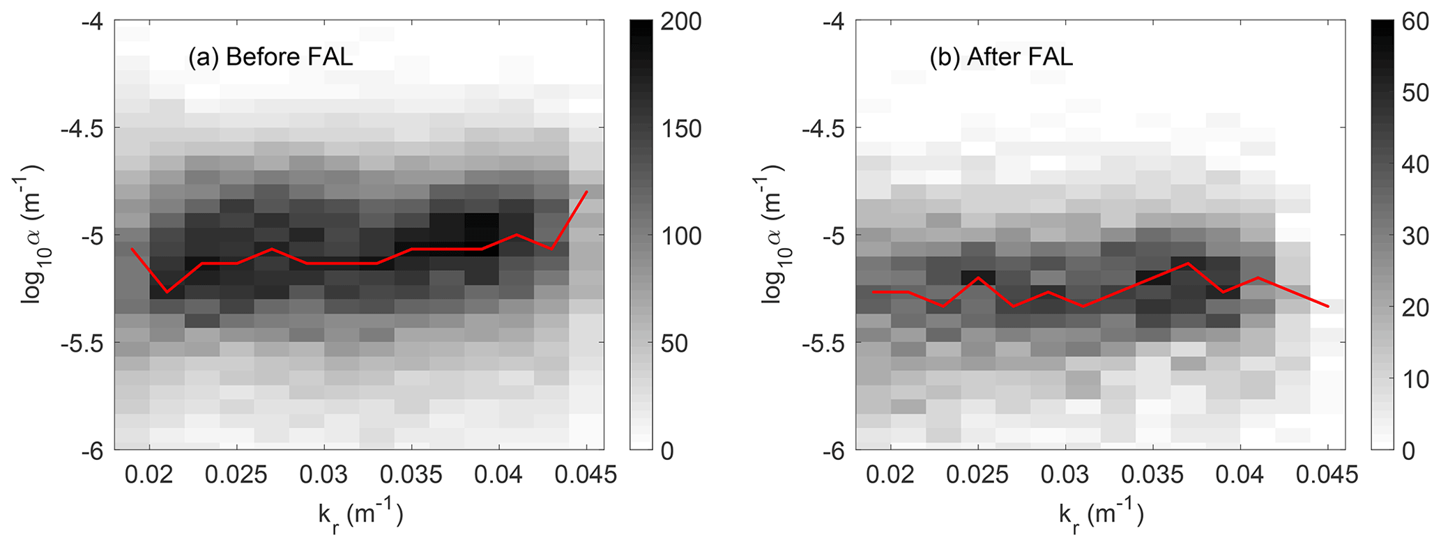
Figure 3 Smoothed two-dimensional histograms of wave number k_r and the apparent attenuation α (a) before the FAL and (b) after the FAL. The α domain is equally divided into 30 bins in the log scale from 10⁻⁶ to 10⁻⁴ m⁻¹. The k_r domain is divided from 0.011 to 0.045 m⁻¹ with an increment of 0.002 m⁻¹. The gray scale indicates the occurrence of α in each α–k_r bin from the selected pairs. The red curve indicates the highest occurrence of α against k_r.

Because of the large study domain and the apparent difference of k_r,dominant in the east–west direction before the FAL, as shown in Fig. 1a, it is worthwhile examining the regional variability. Figure 4 displays the results related to α and k_r in three subdomains from west to east, bounded by longitudes (150, 151^∘ W), (148, 149^∘ W) and (146, 147^∘ W). The left column shows 467, 233 and 132 pairs selected in the three longitude bins, respectively. Each segment indicates a pair selected in Sect. 3.1, with ends corresponding to the locations A and B and its color indicates the mean ice thickness between the two. In the middle column, the α values corresponding to k_r= 0.019, 0.025, 0.031 and 0.039 m⁻¹ obtained from these pairs are separated into two groups: before and after the FAL. In each subdomain delineated by the longitude and the FAL, the distribution of α for each k_r is presented by a violin plot whose width indicates the probability density distribution of α, and a circle marker inside indicates the median. These violin plots show that α before the FAL is larger than that after the FAL for all k_r in all three subdomains. We note that the sample size after the FAL in the easternmost subdomain (146, 147^∘ W) is the lowest, corresponding to the largest variability of the violin plots. To track wave spectrum evolution from near the ice edge towards the interior ice zone, we collect wave PSDs ($\int E\left(k_{\mathrm{r}},\mathit{\theta }\right)\mathrm{d}\mathit{\theta })$ at the north end of each selected pairs in the left column. The averaged PSDs of this collection per 0.1^∘ in latitude are presented by curves in the right column, where colors indicate the latitude. As defined earlier, k_r associated with the peak of a PSD curve is k_r,dominant. Before the FAL the magnitude of the PSD drops rapidly, while k_r,dominant varies slightly as the latitude increases. In contrast, the PSDs change slowly after the FAL, while k_r,dominant decreases quickly. Note that at high latitudes, the PSD at k_r,dominant (red) is higher than that of the same wave number at low latitudes. We revisit this phenomenon in the discussion section.

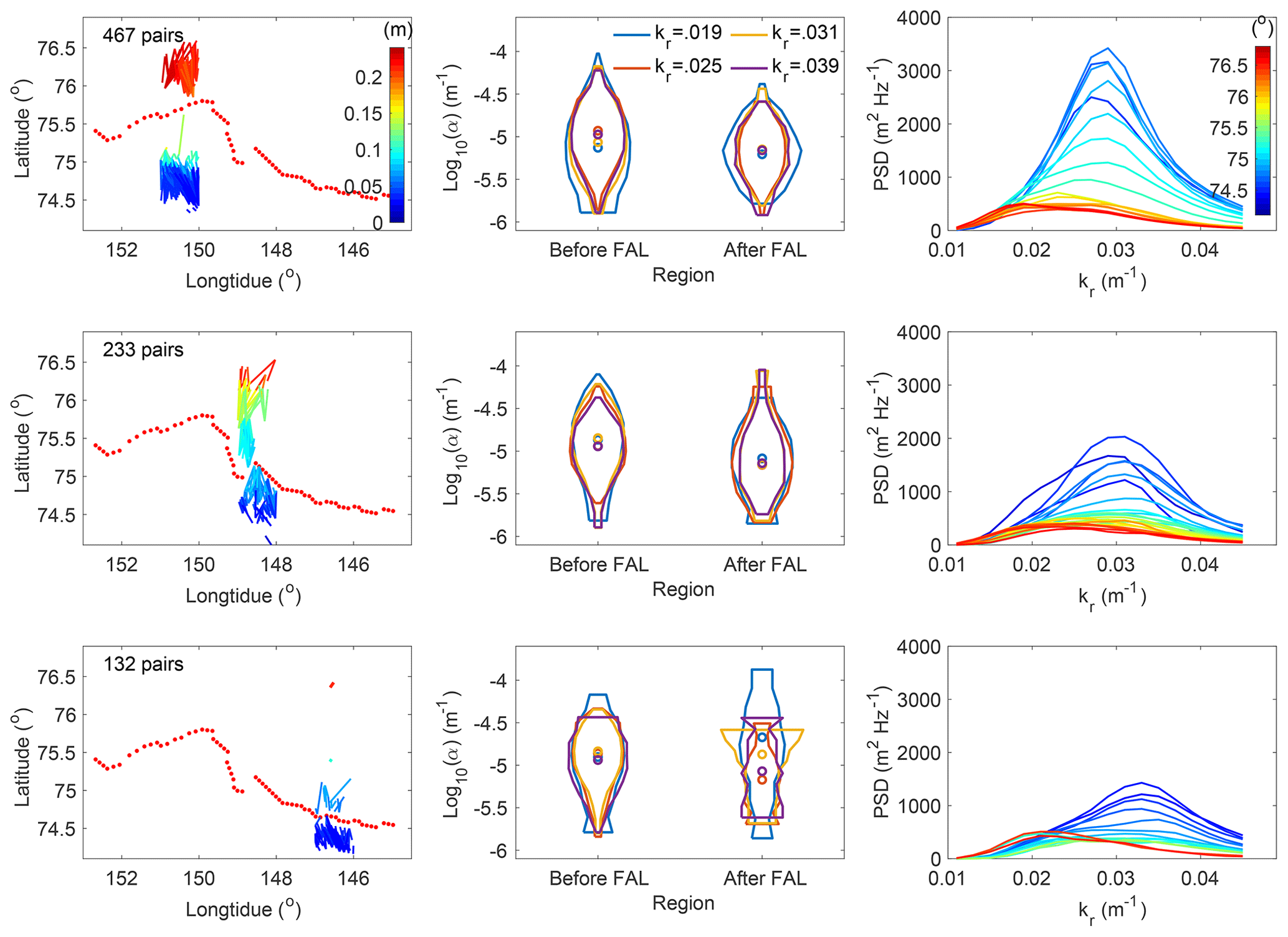
Figure 4 Close view in three selected longitude intervals: (150, 151^∘ W), (148, 149^∘ W) and (146, 147^∘ W). Left column: geographical distribution of the selected pairs, each of which being represented by a segment and color indicating the mean ice thickness. Red dots represent the FAL. Middle column: violin plots of the relevant α, grouped by wave numbers and occurrence before or after the FAL. Right column: evolution of the PSD of wave spectra per 0.1^∘ in latitude. Note that in the rightmost interval (bottom row) the red PSD curves correspond to the few very short red segments near 76.5^∘ N.

3.2 Wave attenuation due to ice effect

Following Eq. (1), the apparent attenuation obtained above is determined by the energy difference between two locations. This apparent attenuation is the result of multiple source terms, including the wind input S_in, damping through wave breaking, and swell dissipation S_ds, the energy transfer due to nonlinear interactions among spectral components S_nl and the dissipation and scattering of wave energy due to ice cover S_ice. In this section, we derive the attenuation rate due to S_ice from the measured apparent attenuation α.

The radiative transfer equation for surface waves concerning all of the above effects is

$$\begin{array}{}\text{(2)}& {\displaystyle \frac{\partial E}{\partial t}}+{\displaystyle \frac{\partial \left(c_{\mathrm{g}}+U\right)E}{\partial x}}=\left(\mathrm{1}-C\right)(S_{\mathrm{in}}+S_{\mathrm{ds}})+S_{\mathrm{nl}}+C{S}_{\mathrm{ice}},\end{array}$$

where $E=E\left(k_{\mathrm{r}},\mathit{\theta },x,t\right)$ is the power spectral density depending on wave number, direction and location x; c_g is the group velocity; and U is the current velocity. Note that U in this region is below 0.1 m s⁻¹ according to OSCAR (Ocean Surface Current Analyses Real-time, ESR, 2009 and Bonjean and Lagerloef, 2002). Because the current speed is at least 1 order of magnitude below the estimated c_g using the open-water dispersion relation, we may drop it from Eq. (2). Furthermore, consistent with the fact that the dispersion relation in this study is close to that of the open water, c_g is relatively constant. Adopting the exponential wave decay along x, i.e., $E\left(k_{\mathrm{r}},\mathit{\theta },x\right)=E\left(k_{\mathrm{r}},\mathit{\theta },x=\mathrm{0}\right)e^{-\mathrm{2}\mathit{\alpha }x}$, we have $\frac{\partial \left(c_{\mathrm{g}}+U\right)E}{\partial x}\approx c_{\mathrm{g}}\frac{\partial E}{\partial x}=-\mathrm{2}{c}_{\mathrm{g}}\mathit{\alpha }E$.

Next, we examine the temporal derivative of wave energy $\frac{\partial E}{\partial t}$. It is challenging to calculate $\frac{\partial E}{\partial t}$ from the nearly instantaneous SAR imagery. Instead, we estimate $\frac{\partial E}{\partial t}$ using hourly wave spectra data from two sources around the time stamp of the SAR imagery: the in situ AWAC-I marked in Fig. 1 and the WW3 simulations of the whole domain (reference model run of Ardhuin et al., 2018). From the AWAC-I data, we obtain $\frac{\partial E}{\partial t}$ and compare that with $c_{\mathrm{g}}\frac{\partial E}{\partial x}$ using SAR-retrieved wave data at the AWAC-I site. From the WW3 simulations, we obtain both terms over the whole study domain. Both results consistently show that $\frac{\partial E}{\partial t}$ is at least 2 orders of magnitude below $c_{\mathrm{g}}\frac{\partial E}{\partial x}$. Thus, $\frac{\partial E}{\partial t}$ is dropped from Eq. (2).

The other source terms S_in and S_ds are estimated using formulations from Snyder et al. (1981) and Komen et al. (1984). For S_nl, we select the discrete interaction approximation (DIA; Hasselmann and Hasselmann, 1985; Hasselmann et al., 1985) to estimate its value. Note that those parameterizations were formulated from an open-water study. How they might change in the presence of ice covers is an open question. The formulations and associated coefficients used here are described in Cheng et al. (2017). Wherever needed in these formulations, f is approximated by the open-water dispersion relation with the measured k_r. Ice concentration is from AMSR2, ice thickness is from SMOS and wind data are from the Climate Forecast System Reanalysis (CFSR; Saha et al., 2010).

Ice-induced wave attenuation is known from the dissipation of wave energy and scattering of waves (e.g., Wadhams et al., 1988; Squire et al., 1995; Montiel et al., 2018). Here we attribute the attenuation entirely to the dissipative process with the following arguments: Ardhuin et al. (2018) reported that in the studied region, ice floe scattering has a weaker effect on wave attenuation compared with other processes, including the boundary layer beneath the ice, inelastic flexing of ice cover and wave-induced ice fracture. The inelastic flexing and ice fracture may be considered as part of the dissipative mechanism within the ice cover already included in the viscous coefficient, but scattering is a redistribution of energy, which must be isolated from the apparent attenuation before using the data to calibrate the viscoelastic models. We estimate the scattering effect based on the study of Bennetts and Squire (2012) as follows: in that study, wave attenuation by floes, cracks and pressure ridges was examined. In the absence of in situ observations, we assume that few and small ridges are present in the studied ice cover (thickness: <0.3 m); hence the effect of ridges is negligible. In our case of long waves propagating through such thin ice cover, Bennetts and Squire (2012) have shown that the floes produce much more attenuation than the cracks. Without in situ observation, WW3 simulations (REF run in Ardhuin et al., 2018) implementing wave-induced fracturing of ice floes gave a range of estimated maximum floe diameter from 70 to 150 m. Using this range of floe diameter, the theoretical scattering results from Bennetts and Squire (2012) indicate that the floe scattering-induced attenuation is about 10⁻⁷ m⁻¹, which is negligible compared to the α shown in Fig. 3.

With all the above simplifications and the assumed exponential decay of wave energy, Eq. (2) becomes

$$\begin{array}{}\text{(3)}& -c_{\mathrm{g}}\mathrm{2}\mathit{\alpha }E=\left(\mathrm{1}-C\right)(S_{\mathrm{in}}+S_{\mathrm{ds}})+S_{\mathrm{nl}}-C\mathrm{2}{c}_{\mathrm{g}}{k}_{\mathrm{i}}E,\end{array}$$

which yields

$$\begin{array}{}\text{(4)}& k_{\mathrm{i}}={\displaystyle \frac{\mathrm{2}{c}_{\mathrm{g}}\mathit{\alpha }E+\left(\mathrm{1}-C\right)\left(S_{\mathrm{in}}+S_{\mathrm{ds}}\right)+S_{\mathrm{nl}}}{\mathrm{2}C{c}_{\mathrm{g}}E}},\end{array}$$

where k_i is the attenuation rate due to the ice cover. The occurrence of the k_i data is presented by two-dimensional histograms of k_i against k_r in Fig. 5. Not surprisingly, since the effect of wind is low due to the low open-water fraction in the study region and the relatively short distances between the pairs for the nonlinear transfer of energy to accumulate, we observe that k_i is very close to the apparent attenuation α. We discuss this ice-induced dissipation further in Sect. 5.

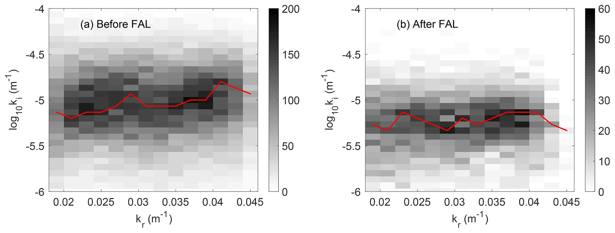
Figure 5 Smoothed two-dimensional histograms of the ice-induced attenuation rate k_i against wave number k_r (a) before the FAL and (b) after the FAL. The attenuation domain is equally divided into 30 bins in the log scale from 10⁻⁶ to 10⁻⁴ m⁻¹. The gray scale indicates the occurrence of k_i in each k_i–k_r bin from the selected pairs. The red curve indicates the highest occurrence of k_i against k_r.

4 Wave-in-ice model calibration

In this section, we present the calibration of the WS model and the FS model. We begin with a brief introduction of the two models then describe the calibration procedure. In both models, k_r and k_i are solved from the respective dispersion relations for given ice thickness and viscoelastic parameters. The viscoelastic parameters are optimized by minimizing the overall difference of the k_i–k_r relationship between the models and data obtained in Sect. 3.

4.1 Dispersion relation

The dispersion relations of the two models are written as

$$\begin{array}{}\text{(5a)}& {\mathit{\sigma }}^{\mathrm{2}}-Qgk\tanh kH=\mathrm{0}.\end{array}$$

For the WS model,

$$\begin{array}{}\text{(5b)}& \begin{array}{rl}& Q=\mathrm{1}+{\displaystyle \frac{{\mathit{\rho }}_{\mathrm{ice}}}{{\mathit{\rho }}_{\mathrm{water}}}}\\ & {\displaystyle \frac{\left(g^{\mathrm{2}}{k}^{\mathrm{2}}-N^{\mathrm{4}}-\mathrm{16}{k}^{\mathrm{6}}{a}^{\mathrm{2}}{\mathit{\nu }}_e^{\mathrm{4}}\right)S_k{S}_a-\mathrm{8}{k}^{\mathrm{3}}a{\mathit{\nu }}_e^{\mathrm{2}}{N}^{\mathrm{2}}(C_k{C}_a-\mathrm{1})}{gk(\mathrm{4}{k}^{\mathrm{3}}a{\mathit{\nu }}_e^{\mathrm{2}}{S}_k{C}_a+N^{\mathrm{2}}{S}_a{C}_k-gk{S}_k{S}_a)}}\end{array}.\end{array}$$

For the FS model,

$$\begin{array}{}\text{(5c)}& Q={\displaystyle \frac{G_{\mathit{\nu }}{h}^{\mathrm{3}}}{\mathrm{6}{\mathit{\rho }}_{\mathrm{water}}g}}\left(\mathrm{1}+V\right)k^{\mathrm{4}}-{\displaystyle \frac{{\mathit{\rho }}_{\mathrm{ice}}h{\mathit{\sigma }}^{\mathrm{2}}}{{\mathit{\rho }}_{\mathrm{water}}g}}+\mathrm{1},\end{array}$$

where H is water depth, σ=2πf is the angular frequency, ρ_ice and ρ_water are the densities of ice and water, respectively, $k=k_{\mathrm{r}}+i{k}_{\mathrm{i}}$ is a complex wave number, h is the ice thickness, $a^{\mathrm{2}}=k^{\mathrm{2}}-\frac{i\mathit{\sigma }}{{\mathit{\nu }}_e}$, S_k=sinhkh, S_a=sinhah, C_k=coshkh, C_a=coshah, $N=\mathit{\sigma }+\mathrm{2}i{k}^{\mathrm{2}}{\mathit{\nu }}_e$, $G_{\mathit{\nu }}=G-i\mathit{\sigma }\mathit{\nu }{\mathit{\rho }}_{\mathrm{ice}}$ and ${\mathit{\nu }}_e=\mathit{\nu }+\frac{iG}{{\mathit{\rho }}_{\mathrm{ice}}\mathit{\sigma }}$ and V is Poisson's ratio. Equivalent shear modulus G and kinematic viscosity ν in both models are to be calibrated. In this study, we use H=1000 m for deep water, ρ_water=1025 kg m⁻³, ρ_ice=922.5 kg m⁻³ and V=0.3 for ice.

Hereafter, we use superscripts t for the theoretical values and m for the measured data. Specifically, the theoretical wave number and attenuation rate are denoted as $k_{\mathrm{r}}^{\mathrm{t}}$ and $k_{\mathrm{i}}^{\mathrm{t}}$. They are calculated for each set of G,ν values. Attenuation data due to the ice effect obtained in Sect. 3 are denoted as $k_{\mathrm{i}}^{\mathrm{m}}$. The corresponding wave number $k_{\mathrm{r}}^{\mathrm{m}}$ is the discretized k_r values from 0.011 to 0.045 m⁻¹ with an increment of 0.002 m⁻¹.

4.2 Calibration methodology

In this section, we optimize G,ν by fitting the k_i–k_r relationship from the model via Eq. (5) to the measured values from Eq. (4). Specifically, for given G and ν, we solve arrays of $k_{\mathrm{r}}^{\mathrm{t}}$ and $k_{\mathrm{i}}^{\mathrm{t}}$ through Eq. (5) for each f densely sampled from 0.0001 to 1 Hz. We then interpolate the results to obtain the theoretical k_i at each wave number $k_{\mathrm{r}}^{\mathrm{m}}$ from the data in Sect. 3.2. For each of these $k_{\mathrm{r}}^{\mathrm{m}}$ we have the measured dissipation rate $k_{\mathrm{i}}^{\mathrm{m}}$ shown in Sect. 3.2. We now use an optimization procedure to determine the best-fit parameters G and ν. The objective function for the optimization is defined as the weighted sum of the differences between $k_{\mathrm{i}}^{\mathrm{t}}$ and $k_{\mathrm{i}}^{\mathrm{m}}$ over $k_{\mathrm{r}}^{\mathrm{m}}$, i.e.,

$$\begin{array}{}\text{(6)}& F={∥w\left(k_{\mathrm{r}}^{\mathrm{m}}\right)\left(k_{\mathrm{i}}^{\mathrm{m}}\left(k_{\mathrm{r}}^{\mathrm{m}}\right)-k_{\mathrm{i}}^{\mathrm{t}}\left(k_{\mathrm{r}}^{\mathrm{m}}\right)\right)∥}_{\mathrm{2}},\end{array}$$

where ∥•∥₂ is the L-2 norm operator and $w\left(k_{\mathrm{r}}^{\mathrm{m}}\right)$ is a weighting factor to account for the distributions of wave energy and attenuation rate. Cheng et al. (2017) tested two weighting factors, $w=\int E\left(\mathit{\theta },f\right)\mathrm{d}\mathit{\theta }$ and $\int E\left(\mathit{\theta },f\right)f^{\mathrm{4}}\mathrm{d}\mathit{\theta }$, in calibrating the WS model. In that study, the measured data had a range of f varied from 0.05 to 0.5 Hz, and the attenuation rate varied from 10⁻⁶ to 10⁻³ m² s⁻¹. The authors found that using $w=\int E\left(\mathit{\theta },f\right)\mathrm{d}\mathit{\theta }$ fitted attenuation best at the most energetic wave band, while $w=\int E\left(\mathit{\theta },f\right)f^{\mathrm{4}}\mathrm{d}\mathit{\theta }$ performed better to capture significant increasing in k_i at high frequencies. No weighting factor could produce a fitting over the entire spectral attenuation curve. For the present study, the variation of spectral attenuation is small, as shown in Fig. 5, with no particular region of emphasis. We thus choose $w=\sqrt{\int E\left(\mathit{\theta },k_{\mathrm{r}}\right)\mathrm{d}\mathit{\theta }}$, which has a broad band around the peak energy of the wave field.

We choose a search domain (10⁻⁷ Pa $\le G\le {\mathrm{10}}^{\mathrm{10}}$ Pa and 10⁻⁴ m² s${}^{-\mathrm{1}}\le \mathit{\nu }\le {\mathrm{10}}^{\mathrm{4}}$ m² s⁻¹) for the WS model. This search domain covers all other reported viscoelastic values for ice covers (e.g., Newyear and Martin, 1999; Doble et al., 2015; Zhao and Shen, 2015; Rabault et al., 2017). For the FS model, it is known that very large G,ν are needed to obtain the level of k_i observed (Mosig et al., 2015). We thus choose a large search domain 10 Pa $\le G\le {\mathrm{10}}^{\mathrm{20}}$ Pa and $\mathrm{10}{\mathrm{m}}^{\mathrm{2}}{\mathrm{s}}^{-\mathrm{1}}\le \mathit{\nu }\le {\mathrm{10}}^{\mathrm{15}}$ m² s⁻¹. This parameter range is far beyond the measured data from solid ice (Weeks and Assur, 1967). The global optimization procedure is performed by using the genetic algorithm with function ga in MATLAB and the Global Optimization Toolbox R2016a (2016).

4.3 Results

For the WS model, the optimized G,ν are gathered into a small cluster around $G\cong {\mathrm{10}}^{-\mathrm{4}}$ Pa and a large cluster around G≅10⁵ Pa, with large variation in ν. The existence of two separate clusters of calibrated results was also found in grease–pancake mixtures near the ice edge (Cheng et al., 2017). Note that multiple solutions (optimized G,ν pairs) could be obtained by optimizing a nonlinear system such as that shown in Eq. (5). Thus, constraints are applied to select solutions that are physically plausible. Note that the solutions around $G={\mathrm{10}}^{-\mathrm{4}}$ Pa and solutions with ν near 10⁴ m² s⁻¹ lead to the residual from Eq. (6) insensitive to G. It implies that the modeled material is viscous-dominant with almost nil elastic effect. Those cases are incompatible with the pack ice condition and are thus removed in the following analysis. Scatter plots of the remaining data points (G,ν) are presented by Fig. S2 in the Supplement. For these remaining data, we apply the bivariate Gaussian distribution to obtain the 90 % probability range of (G,ν) before and after the FAL, respectively. Means and covariances of the related probability density functions are given in Table 1. A slight difference in the distributions of G,ν before and after the FAL is noticed. The mean elasticity is slightly lower before the FAL than after the FAL, and the mean viscosity is slightly higher before the FAL than after the FAL. The results imply that the ice layer behaves more elastic in the inner ice field and more viscous towards the ice edge. It is worth noting that the ranges of both G and ν are about 1 order of magnitude greater than those of the grease and pancake ice (Cheng et al., 2017). As expected, the effective elasticity in the WS model for more solid ice is closer to the elastic modulus of sea ice.

Table 1 Statistical features of the clusters of G and ν from the WS model and FS model calibration. The mean (μ) and covariance (cov) of X=log₁₀G and Y=log₁₀ν.

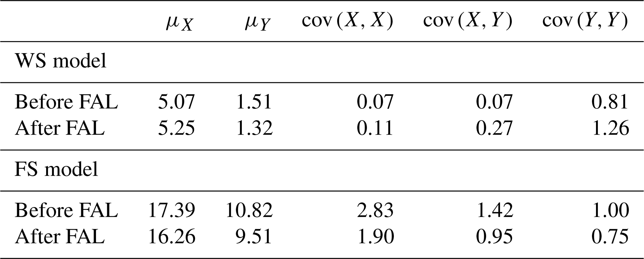
For the FS model, the calibrated (G,ν) are clustered, whereas scatter plots of (G,ν) are given in Fig. S3 in the Supplement. Hence all data points are used in the bivariate Gaussian fitting. The resulting mean and covariance values are also given in Table 1. Notice that the mean values of G, ν from the FS model are extremely larger than the intrinsic values of ice. The distribution of calibrated values is further discussed in the discussion section. Hereafter we only elaborate on the results of the WS model. Figure 6a shows the overall comparison of k_i–k_r between the measurements (gray) and the WS model (black). Both the median (solid curve) and 90 % boundaries (dashed curves) are in good agreement. In Fig. 6a, we superimpose an empirical model from Meylan et al. (2014), which is also included in WW3 to account for the ice effect as switch IC4. By fitting the wave buoy data from the Antarctic MIZ obtained in 2012, Meylan et al. (2014) proposed a simple period-dependent attenuation rate $k_{\mathrm{i}}\left(T\right)=\frac{\mathrm{2.12}\times {\mathrm{10}}^{-\mathrm{3}}}{T^{\mathrm{2}}}+\frac{\mathrm{4.59}\times {\mathrm{10}}^{-\mathrm{2}}}{T^{\mathrm{4}}}$, which is converted into a k_i–k_r relation through the open-water dispersion relation. The empirical formula predicted that attenuation was consistent with the range we obtained here but with a higher sensitivity to k_r. Figure 6b shows the normalized wave number $\frac{k_{\mathrm{r}}}{k_{\mathrm{ow}}}$ against f using the optimized G,ν in the WS model. The deviation of $\frac{k_{\mathrm{r}}}{k_{\mathrm{ow}}}$ from 1 is less than 5 %, indicating the modeled wave dispersion agrees with the open-water dispersion relation. It is consistent with Monteban et al. (2019), who investigated wave dispersion in ice from the SAR data in the Barents Sea as the studied range of wavelength and ice thickness are similar. The counterpart of the FS model is given in Fig. S4 in the Supplement.

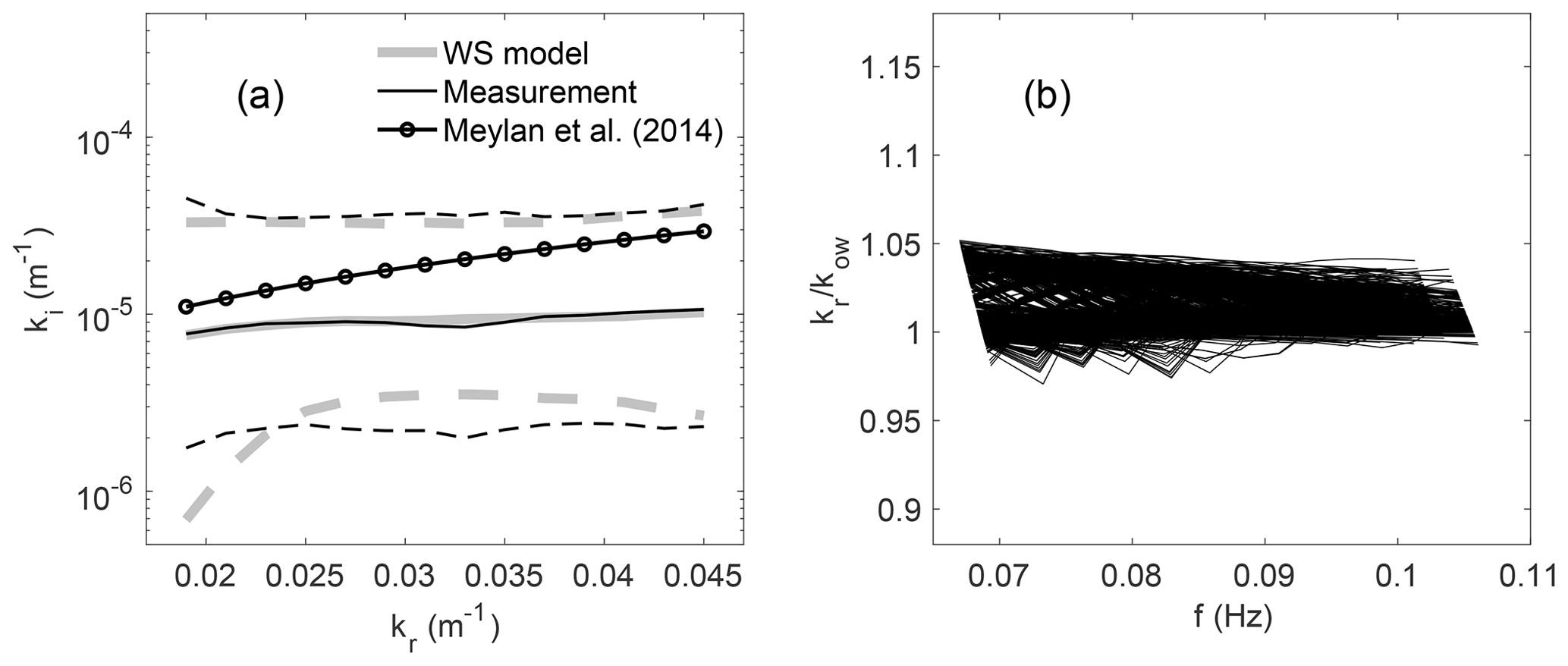
Figure 6 (a) Comparison of ice-induced attenuation k_i between measured data from Eq. (4) and the WS model predictions; solid lines are mean values and dashed lines are 90 % confidence intervals. The thick gray lines are from the calibrated WS model, and the thin black lines are from the data. The black line with the symbol is from the empirical model from Meylan et al. (2014). (b) The corresponding k_r∕k_ow from the calibrated WS model against wave frequency.

Figure 7a, b show distributions of calibrated G and ν from the WS model in the azimuth-range domain, respectively. Contours represent ice thickness distribution from SMOS. The FAL is marked as red dots. The spatial domain is divided into 12.5 km×12.5 km cells to enhance visualization. Cell color indicates the averaged value of log₁₀G and log₁₀ν of all pairs with midpoints inside the cell. Ignoring the outliers, Fig. 7a shows that G is generally larger after the FAL (thicker ice with leads) than before the FAL, while ν has an opposite trend. Note that the outliers could be from multiple sources, such as noise in the retrieved wave data, spatial variability of ice condition, assumptions made in selecting pairs and calculating attenuation and the adopted genetic algorithm in the model calibration. The counterpart of the FS model is given in Fig. S5 in the Supplement.

Figure 7 (a) Distribution of log₁₀G in an averaged 12.5 km×12.5 km grid in the range–azimuth plane. Cell color indicates the averaged log ₁₀G of all pairs with midpoints inside a cell; contours indicate SMOS ice thickness; red dots indicate the FAL. (b) Same as panel (a) except log₁₀G is replaced with log₁₀ν.

5 Discussion

In this section, we discuss some key wave characteristics mentioned in the analysis and the behaviors of calibrated model parameters. Some thoughts about wave-in-ice modeling are provided at the end.

5.1 Evolution of wave characteristics

The behaviors of k_r,dominant and PSD in Figs. 1 and 4 may come from multiple mechanisms. The decrease in k_r,dominant towards the interior ice is in agreement with a similar study in the MIZ (Shen et al., 2018) as well as the lengthening of dominant wave periods reported in many field observations (e.g., Robin, 1963; Wadhams et al., 1988; Marko, 2003; Kohout et al., 2014; Collins et al., 2015). The phenomenon is commonly explained by the low-pass filter mechanism in the literature. That is, higher-frequency waves are preferentially attenuated; thus the power spectrum peak shifts to longer waves. However, though this mechanism is supported by the increasing trend of k_i with increasing wave number before the FAL, it is insufficient to explain the observations after the FAL, where the k_i–k_r curve is practically flat (Fig. 5), and the peak of the PSD shifts toward lower k_r with increasing latitude (Fig. 4). A downshift of wave energy towards lower wave number might also be related to nonlinear wave–wave interaction. Through this interaction, spectral wave energy in the main wave frequency could transfer into the low-frequency components. How to quantify these mechanisms is still an open question, with few data – especially in pack ice – being available and the skills in observations still developing. A piece of critical information is the relationship between the wave period and wave energy, especially in the region after the FAL. Monteban et al. (2019) showed promising applications of overlapping SAR images separated by a sufficient time gap to obtain such information.

The attenuation rate obtained in this study ($\sim {\mathrm{10}}^{-\mathrm{5}}$ m² s⁻¹) against wave number shows a slightly increasing trend before the FAL and a nearly flat trend and lower after the FAL. A similar magnitude of attenuation is found in the MIZ in both the Arctic and Antarctic, as reported in previous studies in the same period range, but larger for shorter periods (e.g., Meylan et al., 2014; Doble et al., 2015; Rogers et al., 2016; Cheng et al., 2017). The analysis of attenuation against wave number in Sect. 3 is obtained for pairs of observations over relatively short distances (<60 km). In Appendix B, we present another method to determine the overall attenuation similar to the analysis of the attenuation of the significant wave height shown in Stopa et al. (2018b). By analyzing wave number by wave number over the entire space that the SAR data covers the apparent attenuation coefficient is obtained by fitting hundreds of data points over long distances, ignoring the higher variation of ice thickness (0.01–0.3 m) and the shift of dominant wave number from the PSD curves. The results are shown in Appendix B, Fig. B2. In some cases, we can even have negative values of this attenuation, meaning energy increases as the wave propagates. What we would like to emphasize by showing this result is that over a very long distance, the ice condition can change significantly in addition to nonlinear energy transfer and wind input and dissipation; thus long-distance spectral analysis may become difficult to interpret.

5.2 About model calibration

The covariance values of the calibrated viscoelastic parameters are greater than those found in grease and pancake ice using buoy data (Cheng et al., 2017). In processing the SAR data, there are many challenges to be dealt with. It is extremely difficult to separate (1) sea ice variability, (2) wave height variability and (3) instrument variability (speckle and incoherent SAR noise). All of these influence the variations we see in the wave spectral data. Still, the scatter of the spectral attenuation shown in Fig. 3 is significant even after the filtering described in Sect. 3.1. This data scatter results in a large range of calibrated model parameters. We believe that the scatter of calibrated G,ν in both WS and FS models could be narrowed down by reducing the uncertainty of measured attenuation data. We also believe that for the FS model the calibrated values and spread could be reduced by modifying the objective function (Eq. 6) with an additional constraint on the wave number, which presently shows an extremely large range as shown in Fig. S4. Regardless, the FS model needs much larger G,ν to produce attenuation rates comparable to the observed data. This is the case not only for the pack ice but also for the MIZ. When analyzing data from the Antarctic MIZ reported in Kohout and Williams (2013) and by further constraining $k_{\mathrm{r}}=k_{\mathrm{ow}}/\mathrm{1.7}$, Mosig et al. (2015) obtained $G=\mathrm{4.9}\times {\mathrm{10}}^{\mathrm{12}}$ Pa, $\mathit{\nu }=\mathrm{5}\times {\mathrm{10}}^{\mathrm{7}}$ m² s⁻¹. Though far below the present case, these values are still orders of magnitude above the intrinsic values measured from solid ice (Weeks and Assur, 1967). Meylan et al. (2018) discussed the attenuation behavior among different dissipative models by assuming small |k_r−k_ow|. Specifically, they showed that the FS model produced $k_{\mathrm{i}}\approx \frac{{\mathit{\rho }}_{\mathrm{ice}}\left(\mathrm{1}+V\right)h^{\mathrm{3}}}{\mathrm{6}{\mathit{\rho }}_{\mathrm{water}}{g}^{\mathrm{6}}}\mathit{\nu }{\mathit{\sigma }}^{\mathrm{11}}$ and the pure viscous case of the WS model (i.e., the model in Keller, 1998) produced $k_{\mathrm{i}}\approx \frac{\mathrm{4}{\mathit{\rho }}_{\mathrm{ice}}h}{{\mathit{\rho }}_{\mathrm{water}}{g}^{\mathrm{4}}}\mathit{\nu }{\mathit{\sigma }}^{\mathrm{7}}$. The higher the power in σ, the more likely ν is to match the measured k_i in the high-period (low-frequency) wave range. The FS model also naturally leads to large G. As shown in Mosig et al. (2015), inverting the dispersion relation shown in Eqs. (5a) and (5c) gives $G-i\mathit{\sigma }{\mathit{\rho }}_i\mathit{\nu }=\mathrm{6}\frac{{\mathit{\rho }}_w{\mathit{\sigma }}^{\mathrm{2}}-gk{\mathit{\rho }}_w-hk{\mathit{\rho }}_i{\mathit{\sigma }}^{\mathrm{2}}}{h^{\mathrm{3}}{k}^{\mathrm{5}}\left(\mathrm{1}+V\right)}$, the leading term of which yields $G\approx O\left(k_{\mathrm{r}}^{-\mathrm{5}}\right)$ in small k_r.

5.3 Thoughts on modeling wave–ice interaction

Damping models play a crucial role in spectral attenuation. At present, using any specific model to describe wave attenuation is tentative. There are many identified damping mechanisms. For instance, boundary layer under the ice cover (Liu and Mollo-Christensen, 1988; Smith and Thomson, 2019), spilling of water over the ice cover (Bennetts and Williams, 2015), interactions between floes (Herman et al., 2019a, b) and jet formation between colliding floes (Rabault et al., 2019) have all been reported in laboratory or field studies. A full wave-in-ice model that considers all important mechanisms is not yet available. While theoretical improvements are needed to better model wave propagation through various types of ice covers, practical applications cannot wait. Calibrated models that are capable of reproducing key observations must be developed parallel to model improvements. The present study provides a viable way to calibrate two such models available in WW3. These models lump all dissipative mechanisms in the ice cover into a viscous term. This type of model calibration study has two obvious utilities. First, with proper calibration, models can capture the attenuation of the most energetic part of the wave spectrum. Second, the discrepancies may be used to motivate the development of models in which there are missing mechanisms, thereby helping future model development. Because different physical processes may play different roles under various ice morphology, collecting wave data to calibrate these models for various ice types is necessary. Finally, more observations with higher-quality data will improve the modeling of the wave–ice interaction and the robustness of the models.

6 Conclusions

In this study, we use the wave spectra retrieved from SAR imagery to examine the spectral attenuation in young pack ice. These images were obtained in the Beaufort Sea on 12 October 2015. According to the analysis of data retrieved over several hundred kilometers, the observed decrease in wave energy and lengthening of dominant waves towards the interior ice are consistent with earlier in situ observations. We investigate wave attenuation of dominant spectral densities per wave number between two arbitrary locations in the region separated by less than 60 km. Similar attenuation rates are observed for all wave numbers from 0.019 to 0.045 m⁻¹ (estimated wave period from 9 to 15 s). After isolating the ice-induced attenuation from these data, we calibrate two viscoelastic-type wave-in-ice models through an optimization procedure between the measured data and theoretical results. Both models can generally match the observed attenuation corresponding to the energetic portion of the wave spectra, with a large difference in dispersion (see wave number plots in Figs. 6 and S4). For the WS model, the calibrated shear modulus and the viscous parameter in the region beyond the first appearance of leads with thicker ice is slightly larger and smaller, respectively, than in the region closer to the ice edge before the first appearance of leads. The resulting wave number is within 5 % of that from the open-water dispersion. The wave–ice interaction is complicated due to many coexisting physical processes. At present no models have fully integrated all identified processes. The present study demonstrates a method based on measured data to calibrate existing models so that they can be applied to meet the operational needs. As the models improve, further calibration exercises may be performed accordingly. For example, the eddy viscosity model (Liu and Mollo-Christensen, 1988) attributed the wave attenuation entirely to the water body under the ice cover. This model is also included in WW3 as the switch IC2, with the eddy viscosity as a tuning parameter. The present analysis can also be used to calibrate that model or models that try to combine both dissipation from the ice cover and the eddy viscosity from the water beneath (e.g., Zhao and Shen, 2018). From a physical point of view, dissipative mechanisms may be present simultaneously inside the ice cover and the water body underneath. However, the calibration of complex models with multiple coexisting processes is a difficult task that requires a much more dedicated study.

We conclude by noting that high-resolution spatial data from remote sensing provide new opportunities to investigate the wave–ice interaction over a large distance and with different ice types. However, details of ice types and temporal observations are in development. To reach a full understanding and thus a complete wave-in-ice model, collaboration from observation and modeling efforts is required.

Appendix A

The definition of the first appearance of leads was introduced in Stopa et al. (2018b). Here we provide more details of the methodology used. The SAR sea surface roughness images in Fig. 1 of Stopa et al. (2018b) are divided into 5.1 km×7.2 km subimages with a 50 % overlap of adjacent subimages in the range–azimuth domain. Each subimage contains 512 pixels×512 pixels. The FAL location for each range position is defined as the minimum azimuth position where large-scale ice features were detected. Detection of large-scale ice features is applied to each SAR subimage as the following. We first compute a one-dimensional spectrum of the SAR subimage to produce an image modulation spectrum. The spectrum is then normalized by the maximum energy contained in wavelengths from 100 to 300 m (the wavelength range of the dominant sea state for this event). When the ratio of the average of the normalized image spectra with wavelengths in the range of 600–1000 m and the dominant ocean wave wavelength range from 160–220 m exceeds 0.8, we deem there to be a “large-scale” feature such as lead within the image. Figure A1 shows two representative examples of detecting ice leads from SAR images captured before and after the FAL. From the criterion above, there are no leads in the top case, but leads are found in the bottom case. Also notice the change in the probability distribution of the roughness: the mean value changes (lower in the nonlead case compared lead case) and the standard deviation (lower in the nonlead case compared to the lead case).

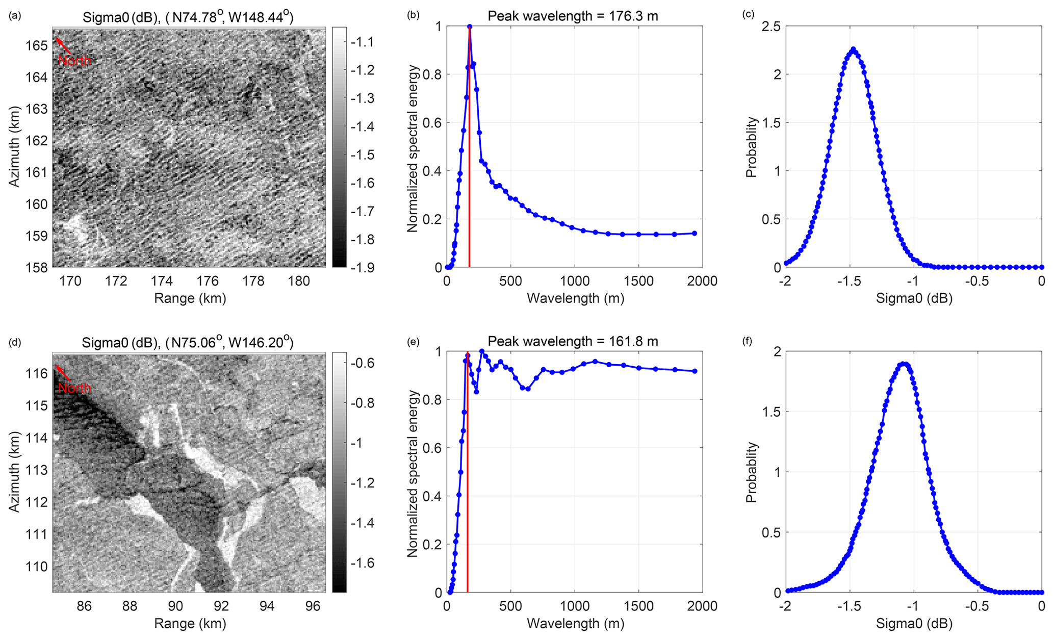
Figure A1 Illustration of the process to determine the FAL using two representative SAR subimages. (a, d) Surface SAR subimage roughness for a case locatedbefore the FAL (a, b, c) and a case located after the FAL (d, e, f). (b, e) Normalized spectral energy (normalized by the maximum energy within the 100–300 m wavelengths) of the SAR subimages, where the red line indicates the dominant wavelength. (c, f) The probability density function of the SAR roughness (backscatter or sigma0 of thermal noise in the SAR imagery) for the two cases.

Appendix B

We investigate the decay of the dominant energy component $E\left(k_{\mathrm{r}},{\mathit{\theta }}_{k_{\mathrm{r}}}\right)$ over a long distance along selected tracks with fixed longitude (145, 146, …, 150^∘ W). Figure B1 shows $E\left(k_{\mathrm{r}},{\mathit{\theta }}_{k_{\mathrm{r}}}\right)$ (blue dots) collected within a given longitude interval 150±0.1^∘ W starting from 74.5^∘ N towards the north. E(k_r) for k_r<0.019 m⁻¹ is too scattered to show any attenuation trend. As k_r increases, the data become tighter with a clear decay trend. To obtain attenuation coefficient $\widehat{\mathit{\alpha }}\left(k_{\mathrm{r}}\right)$, we fit the $E\left(k_{\mathrm{r}},{\mathit{\theta }}_{k_{\mathrm{r}}}\right)$ by an exponential curve (black line) in each panel based on an exponential wave decay assumption.

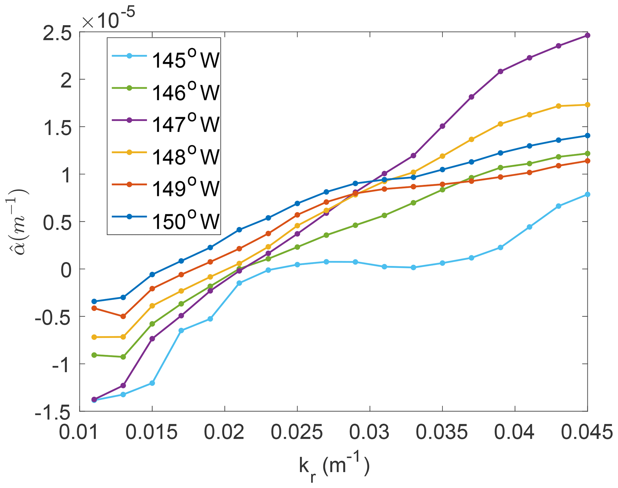
The resulting $\widehat{\mathit{\alpha }}\left(k_{\mathrm{r}}\right)$ against k_r is shown in Fig. B2 as well as another five curves associated with different longitudes, processed in the same way. Figure B2 shows an increasing trend of $\widehat{\mathit{\alpha }}\left(k_{\mathrm{r}}\right)$ against k_r as expected, and $\widehat{\mathit{\alpha }}(k_{\mathrm{r}}<\mathrm{0.019}$ m⁻¹) are mostly negative. This method masks the variation of ice morphology and peak shifting of the power spectral density; thus it is insufficient to understand the damping mechanism in the water–ice interaction. Hence, as our interest is to determine the attenuation in more consistent ice conditions, a shorter distance between measuring points is adopted in Sect. 3.

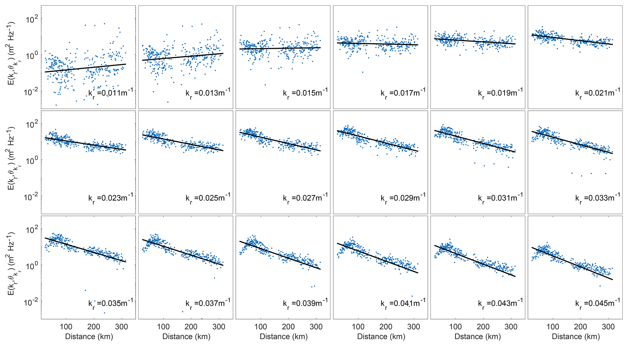
Figure B1 Evolution of dominant wave energy component over long distances within a given longitude interval $\mathrm{150}\pm \mathrm{0.1}{}^{\circ }$ W at different wave numbers. The horizontal axis is the distance along a longitude from 74.5^∘ N towards the north.

Figure B2 $\widehat{\mathit{\alpha }}$ against k_r of different longitude tracks.