Extracting recent short-term glacier velocity evolution over southern Alaska and the Yukon from a large collection of Landsat data

The measurement of glacier velocity fields using repeat satellite imagery has become a standard method of cryospheric research. However, the reliable discovery of important glacier velocity variations on a large scale is still problematic because time series span different time intervals and are partly populated with erroneous velocity estimates. In this study we build upon existing glacier velocity products from the GoLIVE dataset (https://nsidc.org/data/golive, last access: 26 February 2019) and compile a multi-temporal stack of velocity data over the Saint Elias Mountains and vicinity. Each layer has a time separation of 32 days, making it possible to observe details such as within-season velocity change over an area of roughly 150 000 km². Our methodology is robust as it is based upon a fuzzy voting scheme applied in a discrete parameter space and thus is able to filter multiple outliers. The multi-temporal data stack is then smoothed to facilitate interpretation. This results in a spatiotemporal dataset in which one can identify short-term glacier dynamics on a regional scale. The goal is not to improve accuracy or precision but to enhance extraction of the timing and location of ice flow events such as glacier surges. Our implementation is fully automatic and the approach is independent of geographical area or satellite system used. We demonstrate this automatic method on a large glacier area in Alaska and Canada. Within the Saint Elias and Kluane mountain ranges, several surges and their propagation characteristics are identified and tracked through time, as well as more complicated dynamics in the Wrangell Mountains.

1 Introduction

Alaskan glaciers have a high mass turnover rate (Arendt, 2011) and contribute considerably to sea level rise (Arendt et al., 2013; Harig and Simons, 2016). Monitoring changes in ice flow is thus of importance, especially since the velocity of these glaciers fluctuates considerably. Many of the glaciers have been identified as surge type based on direct observations or from their looped moraines (Post, 1969; Herreid and Truffer, 2016). Furthermore, glacier elevation change in this region is heterogeneous (Muskett et al., 2003; Berthier et al., 2010; Melkonian et al., 2014), providing another indication of complicated responses. Gaining a better understanding of causes of glacier mass redistribution is necessary in order to separate surging and seasonal variation from longer-term trends.

Glacier velocity monitoring through satellite remote sensing has proven to be a useful tool to observe velocity change on a basin scale. Several studies have focused on dynamics of individual glaciers in Alaska at an annual or seasonal resolution (Fatland and Lingle, 2002; Burgess et al., 2012; Turrin et al., 2013; Abe and Furuya, 2015; Abe et al., 2016). Such studies can give a better understanding of the specific characteristics of a glacier and which circumstances are of importance for this behavior and response. Region-wide annual or “snapshot” velocities have also been estimated over the Saint Elias mountain range in previous studies (Burgess et al., 2013; Waechter et al., 2015; Van Wychen et al., 2018). The results give a first-order estimate of the kinematics at hand. With frequent satellite data coverage, one study found it is possible to detect the time of glacier speedups to within a week (Altena and Kääb, 2017b), although this study did not include an automated approach. In the most recent work, regional analyses have been conducted over sub-seasonal (Moon et al., 2014; Armstrong et al., 2017) and multi-decadal (Heid and Kääb, 2012a; Dehecq et al., 2015) periods. With such data one is able to observe the behavior of groups of glaciers that experience similar climatic settings. Consequently, surges and other glacier-dynamics events can be put into a wider spatiotemporal perspective.

Since the launch of Landsat 8 in 2013 a wealth of high-quality medium-resolution imagery has been acquired over the cryosphere on a global scale. Onboard data storage and rapid ground-system processing have made it possible to almost continuously acquire imagery. The archived data have enormous potential to advance our knowledge of glacier flow. Extraction of glacier velocity is one of the stated mission objectives of Landsat 8 (Roy et al., 2014). The high data rate far exceeds the possibilities for manual interpretation. Fortunately, automatically generated velocity products are now available (Scambos et al., 2016; Rosenau et al., 2016), though at this point sophisticated quality control and post-processing methods are still being developed.

Up to now, most studies of glacial velocity have had an emphasis on either spatial or temporal detail. When temporal detail is present, studies focus on a single glacier or a handful of glaciers (Scherler et al., 2008; Quincey et al., 2011; Paul et al., 2017). Conversely, when regional assessments are the focus, studies limited themselves to cover a single period with only annual resolution (Copland et al., 2009; Dehecq et al., 2015; Rosenau et al., 2015). Most studies rely on filtering in the post-processing of vector data by using the correlation value (Scambos et al., 1992; Kääb and Vollmer, 2000) or through median filtering within a zonal neighborhood (Skvarca, 1994; Paul et al., 2015). Some sophisticated post-processing procedures are available (Maksymiuk et al., 2016) but rely on coupling with flow models. Alternatively, geometric properties, such as reverse correlation (Scambos et al., 1992; Jeong et al., 2017) or triangle closure (Altena and Kääb, 2017a), can be taken into account during the matching to improve robustness and reduce post-processing efforts.

While glacier velocity data are increasingly available, in general post-processing is not at a sufficient level to directly exploit the full information content within these products. In this study we describe the construction of a post-processing chain that is capable of extracting temporal information from stacks of noisy velocity data. Our emphasis is on discovering temporal patterns over a mountain-range scale. Analysis of the details of glacier-dynamics patterns identified by this processing will be considered in later work. For a single glacier, it is certainly possible to employ manual selection of low-noise, good-coverage velocity datasets. However, such a strategy will not be efficient when multiple glaciers or mountain ranges are of interest. In this contribution we want to develop the methodological possibilities further and try to construct glacier velocities at a monthly resolution over large areas. Therefore, our implementation focuses on automatic post-processing, without the help of expert knowledge or human interaction. Our method retains spatial detail present in the data and does not simplify the flow structure to flow lines. This methodology can generate products that improve our knowledge about the influence and timing of tributary and neighboring ice flow variations.

We start by discussing the data used and provide background on the area under study. We then introduce the spatiotemporal structure of the data, followed by an explanation of our process for vector “voting” and vector field smoothing. The final section highlights our results and our validation and assessment of the performance of the method.

2 Data and study region

2.1 GoLIVE velocity fields

The Global Land Ice Velocity Extraction from Landsat 8 (GoLIVE) velocity fields used in this study are based upon repeat optical remote-sensing imagery and are distributed through the National Snow and Ice Data Center (NSIDC; https://nsidc.org/data/golive, last access: 26 February 2019) (Scambos et al., 2016). These velocity fields are derived from finding displacements between pairs of Landsat 8 images, using the panchromatic band with 15 m resolution. A high-pass filter of 1 km spatial scale is applied before processing. Normalized cross-correlation is applied between the image pairs on a sampling grid with 300 m spacing (Fahnestock et al., 2016; Scambos et al., 1992) and a template size of 20 pixels (or 300 m). The resulting products are grids with lateral displacements, the absolute correlation value, signal-to-noise ratio and ratio between the two best matches. At the time of writing, displacement products can cover a time interval from 16 days up to 96 days. For a detailed description of the processing chain see Fahnestock et al. (2016).

The Landsat 8 satellite has a same-orbit revisit time of 16 days and a swath width of 185 km. Only scenes which are at least 50 % cloud-free are used (as determined by the provided estimate in the metadata for the scenes). Consequently, not every theoretical pair combination is processed, and no pairs of overlapping images with different orbits (paths) are used (see Altena and Kääb, 2017a) to avoid more complicated viewing geometry adjustments. Georeference errors are compensated for by the estimation of a polynomial bias surface through areas outside glaciers (i.e., assumed stable). The glacier mask used for that purpose is from the Randolph Glacier Inventory (RGI) (Pfeffer et al., 2014). The resulting grids come in Universal Transverse Mercator (UTM) projection and if orthorectification errors are minimal, displacements for precise georeferencing require only horizontal movement of a few meters (generally <10 m). In total we use 12 Landsat path–row tiles to cover our study area (Fig. 1).

2.2 Study region

The region of interest covers the Saint Elias, Wrangell and Kluane mountain ranges, as well as some parts of the Chugach range. Many surge-type glaciers are located in the Saint Elias Mountains (Post, 1969; Meier and Post, 1969). These ranges host roughly 42 000 km² of glacier area with roughly 22 % of the glacier area connected to marine-terminating fronts draining into the Gulf of Alaska (Molnia, 2008). The glaciers in this area are diverse, as a wide range of thermal conditions (cold and warm ice) and morphological glacier types (valley, ice fields, marine terminating) occur in these mountain ranges (Clarke and Holdsworth, 2002). This diversity is in part due to the large precipitation gradient over the mountain range. The highest amount of precipitation falls in summer or autumn. The study area covers mountain ranges with two distinct climates. Along the coast one finds a maritime climate with a small annual temperature range. These mountains function as a barrier, and the mountain ranges behind, in the interior, have a more continental climate (Bieniek et al., 2012).

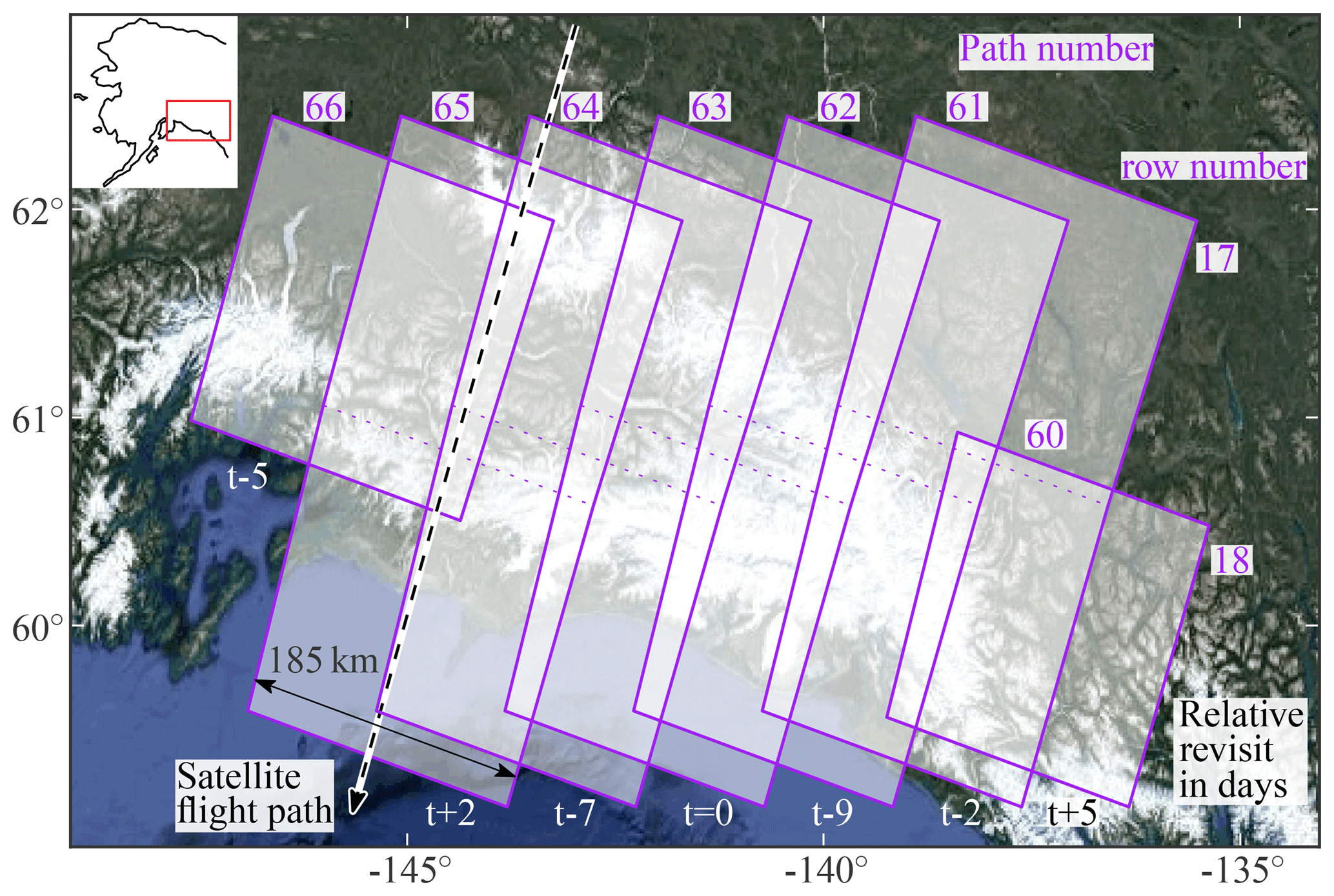
Figure 1 Nominal Landsat 8 footprints used over the study region. The purple text annotates the different satellite paths of Landsat, while the white text indicates the relative overpass time in days with respect to path 63.

3 Methodology

GoLIVE and other similar velocity products are derived from at least two satellite acquisitions. When images from multiple time instances are used, combinations of displacements, with different (overlapping) time intervals, can be constructed. In order to be of use for time series analysis, detailed velocity fields with different time spans need to be combined into a dataset with regular time steps. To reduce the noise, the temporal configuration of overlapping products can be used to synthesize am improved multi-temporal velocity field.

3.1 Temporal network configuration

At the latitude of southern Alaska, scenes from adjacent tracks have an overlap of 60 %. Looking at one track only (or Landsat path), the 16-day revisit makes several matching combinations of integer multitudes of 16 days possible. For example, suppose that over a 64-day period (Δt), five images are acquired from one satellite track and their potential pairing combinations can be illustrated as a network (Fig. 2). In this network, every acquisition (at time t) is a node, and these nodes are connected through an edge that represents a matched pair leading to a collection of displacements (d) with associated similarity measures (ρ).

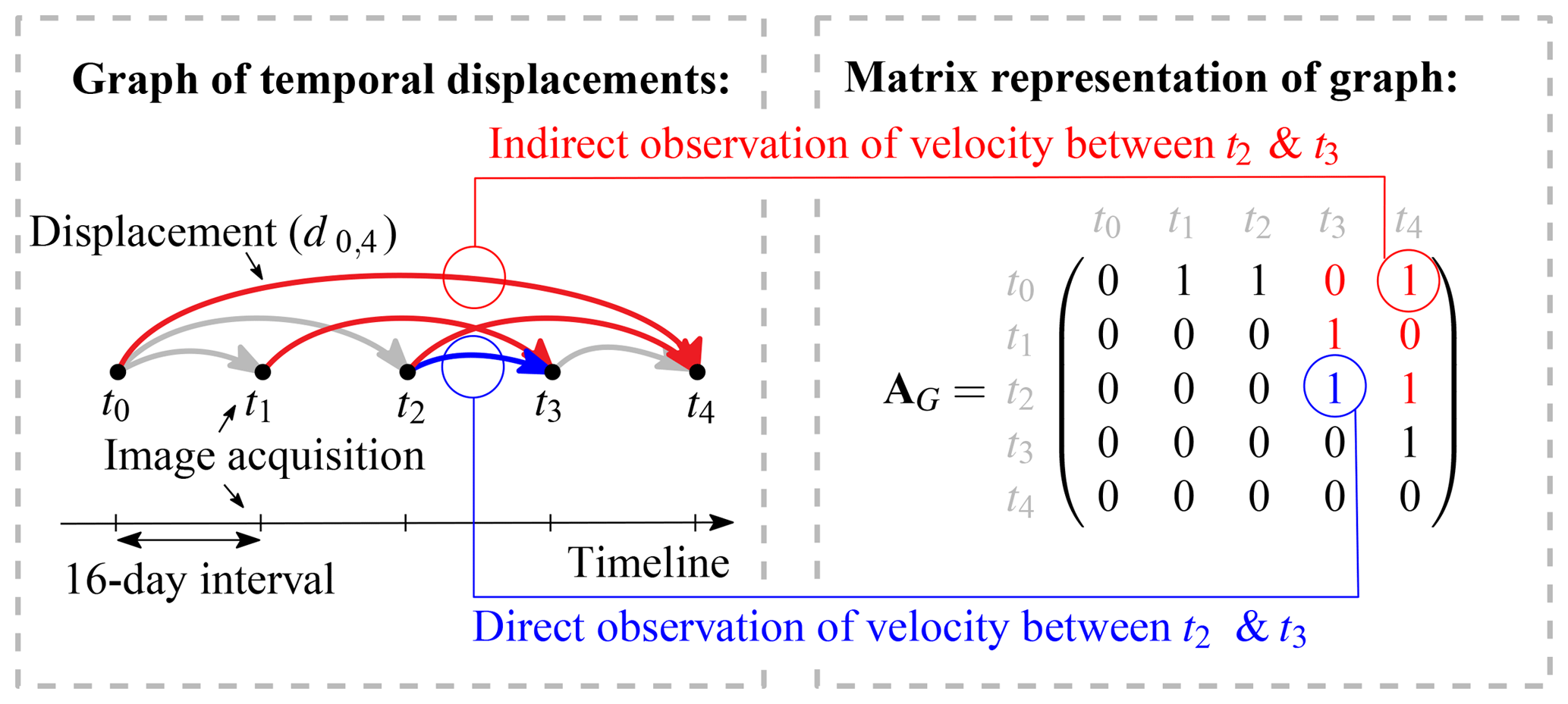
Figure 2 Graphical and matrix representation of a network. Here acquisition pairs within a network are illustrated and written down in an adjacency matrix (A_G). The dark gray squares indicate acquisitions within a period to be estimated. The connecting colors symbolize an open (red) or closed (blue) selection of displacements to be used for the velocity estimation over this period (v).

When velocities over different time spans are estimated, this network has in theory a great amount of redundancy. However in practice this is complicated, as combinations of images are not processed when there is too much obstruction by clouds. Furthermore, individual displacements can have gross errors, as an image match was not established due to surface change or lack of contrast and thus loss of similarity. Consequently, when data from such a network are combined to synthesize one consistent velocity time series, the estimation procedure needs to be able to resist multiple outliers or be able to identify whether displacement estimates could be extracted at a reliable level at all.

The network shown in Fig. 2 can be seen as a graph; nodes correspond to time stamps and edges to matched image pairs. Such a graph can be transformed into an adjacency matrix (A_G, see Fig. 2). In this matrix the columns and rows represent different time stamps. The edges can be directed, indicating which acquisition is the master (reference) or the slave (search) image during the matching procedure. For the GoLIVE data, the oldest acquisition is always the reference image; hence within the matrix only the upper triangular part has filled entities. The spacing of the time steps is 16 days and the number of days is set into the corresponding entries when a time step is covered by an edge. Individual days are specified so that adjacency matrices from different tracks which have different acquisition dates can be merged. If partial overlap of an edge occurs, then the time steps are proportionally distributed. For example, for a small network of three nodes, velocity (v) can be estimated through least-squares adjustment of the displacements (d) through the following systems of equations (Altena and Kääb, 2017a):

$$\begin{array}{ll}{\displaystyle }\mathit{y}=\mathbf{A}\mathit{v},\text{where}& {\displaystyle }\mathit{y}=\left[\begin{array}{c}{d}_{\mathrm{12}}{d}_{\mathrm{23}}\\ d_{\mathrm{13}}\end{array}\right],\mathbf{A}=\left[\begin{array}{cc}\mathrm{\Delta }{t}_{\mathrm{12}}& \mathrm{0}\\ \mathrm{0}& \mathrm{\Delta }{t}_{\mathrm{23}}\\ \mathrm{\Delta }{t}_{\mathrm{12}}& \mathrm{\Delta }{t}_{\mathrm{23}}\end{array}\right],\\ \text{(1)}& {\displaystyle }& {\displaystyle }\mathit{v}=\left[\begin{array}{c}{v}_{\mathrm{12}}\\ v_{\mathrm{23}}\end{array}\right].\end{array}$$

Here the subscript denotes the time span given by the starting and ending time stamps of the interval. This relational structure of displacements is similar to a leveling network. When the adjacency matrix is converted to an incidence matrix, then this matrix is the design matrix (A) (Strang and Borre, 1997). This makes the generation of such network adjustments easily implemented.

This formulation of the temporal network makes it possible to estimate the unknown parameters, i.e., the temporal components of the velocity time series, through different formulations. This is illustrated in Fig. 2, in which a velocity (between t₂ and t₃) is estimated. Displacements that fall between the two images can be used for the estimation (here blue), which we here call a “closed” network. But as can be seen in the figure as red connections, other displacements from outside the time span are overarching and stretching further than the initial time interval. Such measurements can be of interest as they can fill in gaps or add redundancy, but the glacier flow record obtained will be aliased compared to the real motion. Consequently, we call such a network configuration an “open” network (here red).

3.2 Voting

The velocity dataset we use (like any) contains a large number of incorrect or noisy displacements. Typically, the distribution of displacements has a normal distribution but with long tails. Moreover, a least-squares adjustment is very sensitive to outliers contained in the data to be fitted. Therefore, direct least-squares computation of velocity through the above network is not easily possible and some selection procedure is needed to exclude gross errors. Outlier detection within a network such as in Eq. (1) can be performed through statistical testing (Baarda, 1968; Teunissen, 2000), assuming measurements (d) are normally distributed. However, such procedures are less effective when several gross errors are present within the set of observations. Extracting information from highly contaminated data is therefore an active field of research. For example, robust estimators change the normal distribution to a heavy-tailed distribution. Nevertheless, such estimations typically still start with a normal least-squares adjustment based on the full initial set of observations, and only in the next step are the weights iteratively adjusted according to the amount of misfit. Hence, such methods are still restricted to robust a priori knowledge or a dataset with relatively small amounts of contamination by gross errors.

Another common approach to cope with the adjustment of error-rich observations is through sampling strategies such as least median of squares (Rousseeuw and Leroy, 2005), or random sampling and consensus (RANSAC) (Fischler and Bolles, 1981). A minimum number of observations are picked randomly to solve the model. The estimated parameters are then used to assess how the initial model fits with respect to all observations. Then the procedure is repeated with a new set of observations. The sampling procedure is stopped when a solution is within predefined bounds, or executed a defined number of times after which the best set is taken. Such methods are very popular as they can handle high contamination of data (up to 50 %) and still result in a correct estimate. Put differently, the breakdown point is 0.5 (Rousseeuw and Leroy, 2005). However, we use a different approach as these methods implement polynomial models. Our dataset benefits from including conditional equations as well.

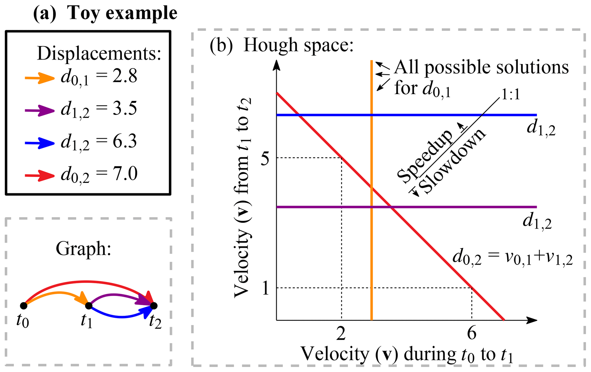
Figure 3 On the left is a graphical representation of Landsat 8 acquisitions at different times (t) illustrated as nodes and matching solutions with displacements (d) are shown as edges, within a network. The subscript for the displacement denotes the time interval. The velocities (v) are estimated through the collection of all these displacements. On the right the mathematical representation or its parameter (Hough) space for voting of displacements over two time instances is shown; in this case the parameter space of only v_0,1 and v_1,2 are shown.

The equations that form the model can be seen as individual samples that populate the parameter space. In such a way the individual relations within the equation propagate into points, lines or surfaces depending on their dimensions and relation given by the equation. Hence, measurements can be transformed into a shape that is situated within the parameter space (which has a finite extent and resolution). The collection of shapes will be scattered throughout this parameter space, but such shapes converge at a common point, which is most likely the correct parameter values. This transformation is the Hough transform and is commonly used in image processing for the detection of lines and circles.

However, the Hough transform is discrete while the measurements are noisy; thus the shapes should also be fuzzy. In this study we follow this latter direction and after discretizing the displacement-matching search space, we exploit a voting strategy. Because the shapes in parameter space are blurred, a fuzzy Hough transform (Han et al., 1994) is implemented. Our matching search space is simply the linear system of equations of the network described above. To illustrate the system, an example of a network with four displacements (d) is shown in Fig. 3. These displacements can be placed within a discrete grid that spans a large part of the parameter space (in this example two dimensional). For the short time span displacements, this results in vertical or horizontal lines (blue, purple and orange). The lines originate from the ambiguity, which is also in the entries of the design matrix (A) as 0 entries. For the overarching displacement (in red) the displacement is a combination of both velocities. Only the total displacement is known; thus the line results in a diagonal orientation (5+2 can be a solution as well as 1+6, or a non-integer combination).

In this toy example, the lines concentrate around 3 for both velocities, but with a slight preference to the upper left. This location indicates a slight speedup between these two time spans. For this case, the blue line is an outlier; it does not contribute to crossings in this zone and instead creates single crossings with other correct displacements at other locations within the parameter space. Apart from the blue line, the other crossings are concentrated around a zone but do not perfectly intersect at a single point. This is due to noise present in every displacement measurement. To simulate this noise, the lines are perturbed with a Gaussian function, as for the toy example shown in Fig. 4a. In this case, every observation will fill the parameter space with a discretized weighting function. This fuzziness in the Hough space makes it possible to find the intersection while noise is present. The dimension of the Hough space depends on the formulation of the network. In principle it can have any dimension; in one dimension this is a simple histogram, but in higher dimensions this will translate into a line which radially decreases in weight. For this study we implement a three-dimensional Hough space, which for our toy example will look like Fig. 4b; though due to visualization limitations, the fuzzy borders are not included.

The advantage of a Hough search space is the resistance to multiple outliers. It builds support and is not reliant on the whole group of observations. When a second or third dimensional space is used, the chances of random (line) crossing decrease significantly in the parameter space, and such events will stand out when multiple measurements do align. Random measurement errors can be incorporated through introducing a distribution function. In our implementation this is a Gaussian distribution, but other functions are possible as well. The disadvantage of the fuzzy Hough transform is its limitation in implementing a large and detailed search space, as the dimension and resolution depend on the available computing resources.

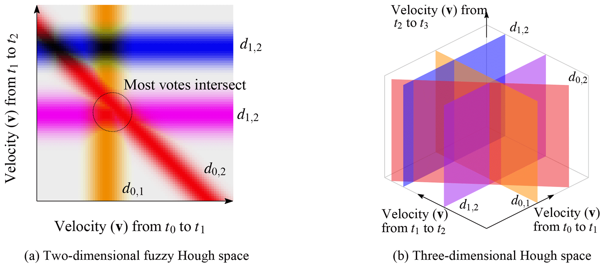
Figure 4 Two modifications used in this study, which deviate from the standard Hough transform as given by the toy example in Fig. 3. (a) The change from a clear ideal line towards fuzzy weights. (b) The extension towards a higher dimension, in this case the lines transform to planes that intersect with each other.

The fuzzy Hough transform functions as a selection process to find observations which are to a certain extent in agreement. With this selection of inliers the velocity can finally be estimated through ordinary least-squares estimation. The model is the same as used to construct the network. However, the observations without consensus (i.e., outliers) are not used. The remaining observations can, nevertheless, still be misfits, such as from shadow casting, as no ice flow behavior is prescribed in the design matrix of Eq. (1).

3.3 Smoothing

Because the voting and least-squares adjustment in our implementation has no neighborhood constraints but is rather strictly per matching grid point, the velocity estimates contain systematic, gross and random errors, though reduced with respect to the initial dataset. This least-squares adjustment with voted displacements results in a spatiotemporal stack of velocity estimates that have a regular temporal spacing. However, due to undersampling as a result of cloud cover or lack of consensus among the displacement acquisitions, the stack might have holes or ill-constrained estimates. We apply a spatial–temporal smoothing taking both spatial and temporal information into account using the Whitacker approach that tries to minimize the following function (S),

$$\begin{array}{}\text{(2)}& S=\sum _i{w}_i({\widehat{x}}_i-x_i{)}^{\mathrm{2}}+\mathit{\lambda }\sum _i({\mathrm{\Delta }}^{\mathrm{2}}{x}_i{)}^{\mathrm{2}}.\end{array}$$

This formulation is the one-dimensional case, in which for every location (x, where i denotes the index of the grid) an estimate (denoted by $\widehat{\cdot }$) is searched for that minimizes S. Here Δ denotes the difference operator; thus $\mathrm{\Delta }{x}_i=x_{i+\mathrm{1}}-x_i$. Similarly, Δ² is the double difference, describing the curvature of a signal (${\mathrm{\Delta }}^{\mathrm{2}}{x}_i=x_{+\mathrm{1}}-\mathrm{2}{x}_i+x_{i-\mathrm{1}}$). For the implementation of this method we use the procedure presented by Garcia (2010). This routine has an automatic procedure to estimate the smoothing parameter (λ) and has robust adaptive weighting (w). Its implementation uses a discrete cosine transform (DCT), which eases the computational load. The discrete cosine transform operates both globally and locally, and in multiple dimensions. In order to include all data at once, the vector field is configured as a complex number field.

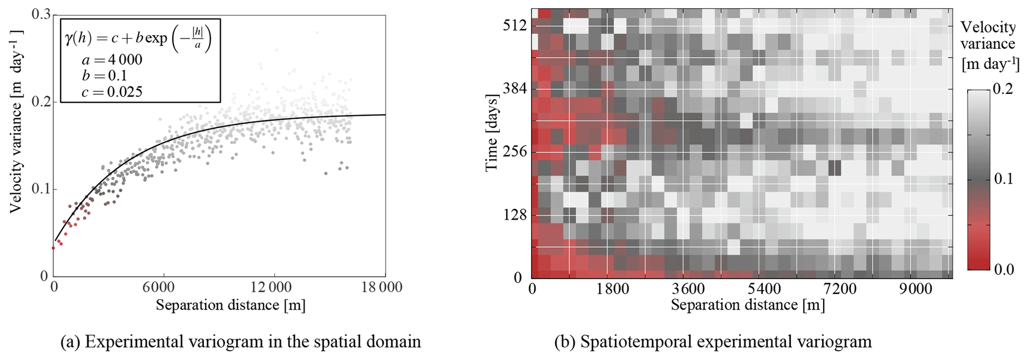
Figure 5 Experimental variograms over a slice of the stack and over a subset of the spatiotemporal stack. The color bar along the axis of (a) is used for the coloring of (b). The aspect ratio of panel (b) is at the resolution of the produced data cube (32 days by 300 m). In order to make this isotropic, the vertical axis needs to enlarge, so the spread in variance is similar in any direction (isotropic).

The smoothing parameter (λ) operates over both space (two dimensions) and time (one dimension), but the smoothing parameter is a single scalar. In this form it would be dependent on the choice of grid resolutions in time and space. In order to remove this dependency and fulfill the isotropy property, the spatial and temporal dimensions are scaled. For this scaling estimation we construct an experimental variogram and look at its distribution (Wackernagel, 2013). A subsample of the dataset with least-squares velocity estimates is taken for this purpose, which is situated over the main trunk and tributaries of Hubbard Glacier. Along the spatial axis, the variogram in Fig. 5a shows spatial correlation up to about 10 km. This sampling interval is then used to look at the spatiotemporal dependencies, as illustrated in Fig. 5b. At around a year in temporal distance one can see a clear correlation which corresponds to the seasonal cycle of glacier velocity. From this variogram a rough scaling was estimated, and the anisotropy was set towards a factor of 4. In our case the pixel spacing is 300 m and the time separation is 32 days.

4 Results

4.1 Method performance

Two different temporal networks (combinations of time intervals) can be formulated in order to calculate a velocity estimate, as is described in Sect. 3.1. The open configuration includes a greater number of velocity estimates from image pairs, but this has consequences. It results in a more complete dataset, with coherent velocity fields, but when short-term glacier dynamics occur, temporal resolution of the event may be aliased.

Our methodology thrives when several displacement estimates are present; otherwise testing is not possible. This prerequisite is especially apparent when a closed configuration is used; then the collection of displacements are reduced. In order to show this dependency a slice is shown in Fig. 6. In this time interval the western side has several overlapping displacement estimates in space and time, while this is limited at the eastern side. The exact distribution of the available data for this time interval is also highlighted in Fig. A1, within Appendix A. The lack of data can be seen at the western border of both estimates. On the eastern side the glacier velocity structure is more clearly visible, especially in the open configuration.

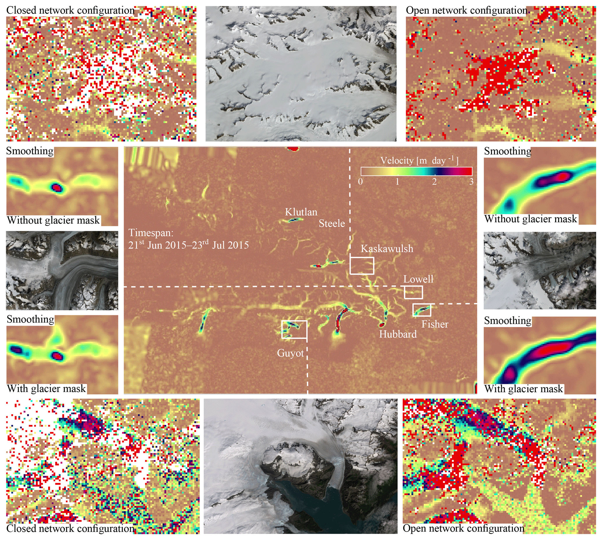
In Fig. 7 more details of the two different configurations are shown. By including more imagery as with an open configuration, the velocity estimates are more complete, as can be seen along the outlets of Guyot Glacier. In the same subsection, the completeness increases and so does the consistency, which is most apparent in the coherent low velocities over stable ground. With more displacement vectors in the configuration, smaller-scale details, such as tributaries flowing into the large Kaskawulsh Glacier, become more evident.

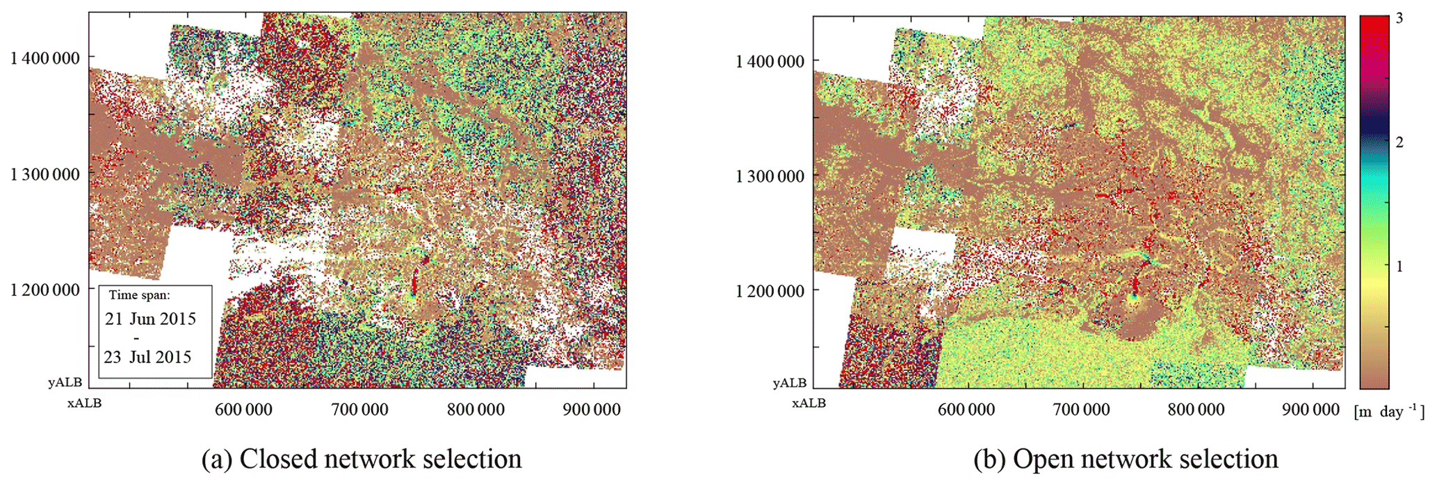
Figure 6 Least-squares estimates of velocities for the region shown in Fig. 1 with different network configurations. See Fig. 3 for a toy example of the terminology. The study region is spread over several UTM zones; hence the dataset is in Albers equal-area projection (ALB) with North American Datum 83. White regions correspond to data without an estimate.

The spatiotemporal least-squares estimates still have, to some extent, variation in direction and amplitude as well as outliers. Therefore spatial–temporal smoothing is applied, in order to extract a better overview from the data, as is described in Sect. 3.3. The results of this smoothing for the same time interval as in Fig. 6 are shown in Fig. 7.

In the smoothing procedure the surroundings of glaciers, which are stable or slow-moving terrain, are included. Consequently, high speedups such as on the surge bulge on the Steele Glacier are dampened, as in this case it has a confined snout within a valley. They do not disappear, as the signal is strong and persistent over time, but damping does occur. An aspect of concern is the retreat of the high-velocity termini of many outlet glaciers; their fronts with large velocities seem to retreat in the smoothed version, while this is not the case for the original least-squares estimate (see example in Appendix B). This effect is caused by surrounding zero-valued water bodies. Damping also occurs at turns such as at Hubbard Glacier, where the mask reduces the effect of stable terrain but has no specific glacial properties. The isotropy function included in the smoother might work for a local neighborhood but breaks down for fast-moving outlets. For this smoother, weights are given in relation to a neighborhood. However for glacier flow, the magnitude might be more similar in the direction of flow lines, while in the cross-flow direction the flow orientation might be more similar. This relation is not included in the smoother, causing damping of the gradients. There is a trade-off between the damping effect of the smoothing and the advantage of having a clear image over large areas.

Because the surrounding terrain, which has no movement, impacts the smoothed glacier velocity estimates, in particular for surge and calving fronts (i.e., for strong spatial velocity gradients), the smoothing can be supported by a glacier mask. In our case, this mask is a rasterization of the Randolph Glacier Inventory (Pfeffer et al., 2014), with an additional dilation operation, to take potential advance or errors in the inventory into account. The difference in result using this masking procedure is shown in Fig. 7, with some highlights. In general, the mask does compensate a little bit for the damping, but because the regions are mostly covered with ice its effect is small.

Figure 7 Overview map of different sections for the time interval, which is similar to Fig. 6 (i.e., 21 June till 23 July 2015). The surrounding zoom-ins are from the same time period but with different configurations (open vs. closed) or smoothing settings (glacier mask vs. no mask).

4.2 Validation over stable terrain

A first component for validation is an analysis of the stable ground and the effect of the smoothing of the voted estimates. The non-glaciated terrain is taken from a mask. A similar mask, also based on the Randolph Glacier Inventory, is used within the GoLIVE pipeline. Here, displacements over land and non-glaciated terrain are used to co-align the imagery (Fahnestock et al., 2016), as geo-location errors might be present in the individual Landsat images. The fitting is performed through a polynomial fit; in general these offsets should be random with a zero mean.

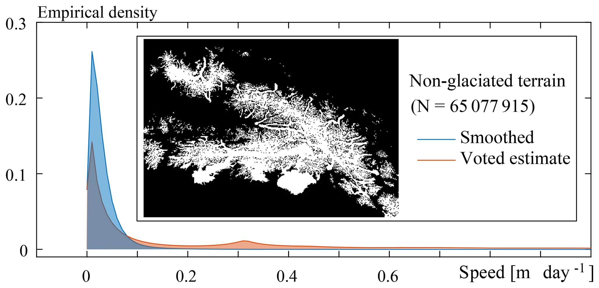
Figure 8 Distribution of the speed over stable terrain, for displacements extracted from the voting process, or after spatial temporal smoothing. The mask used is within the inset.

The distribution of these stable terrain measurements, more than 65 million in total, are illustrated in Fig. 8. Similar to the visual inspection already illustrated in Fig. 6b, the distributions also show a clear improvement, even though the voted estimates still seem to be noisy with significant outliers.

4.3 Validation of post-processing procedures

The voting used in our procedure is assessed through validation with an independent velocity estimate. Terrestrial measurements are limited in the study area; hence we use satellite imagery from RapidEye satellites over a similar time span. Data from this constellation have a resolution of 5 m and through processing in a pyramid fashion, a detailed flow field can be extracted. This velocity field functions as a baseline dataset to compare the GoLIVE and the synthesized data. Here we will look at a section of Klutlan Glacier, which flows from west to east and is thus aligned with one map axis. The velocity of this glacier is, due to its surge, of significant magnitude and therefore will have a wide spread in the voting space.

The two RapidEye images used over Klutlan Glacier were taken on 7 September and on 7 October 2016. To retrieve the most complete displacement field of the glacier, we used a coarse-to-fine image matching scheme. The search window decreased stepwise (Kolaas, 2016) and the matching itself was carried out through orientation correlation (Heid and Kääb, 2012a). At every step a local post-processing step (Westerweel and Scarano, 2005) was implemented to filter outliers. The resulting displacement field over one axis (that is x, the general direction of flow) for this period is illustrated in Fig. 9a.

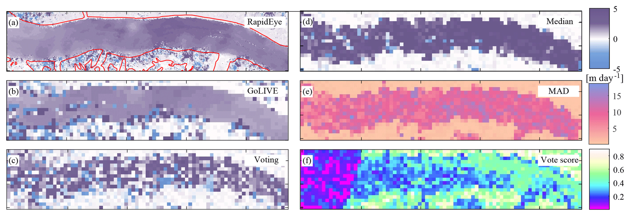
Figure 9 Monthly displacement in the x direction over the Klutlan Glacier (for location see Fig. 7) using several data sources and velocity assessment schemes. Panel (a) shows velocities derived from two RapidEye images. Glacier borders are outlined in red. Panel (b) shows displacement estimates from a GoLIVE dataset (input) and the resulting voted estimate (c) of a combination of 36 GoLIVE datasets (output). The corresponding voting score of these estimates is shown in (f). Panels (d) and (e) show the median and the median of absolute deviation (MAD), respectively, over the full dataset. These last two results would typically be used for data exploration.

For the voting of the Landsat 8-based GoLIVE data, an overlapping time period was chosen, from 11 September up to 13 October 2016, nearly but not exactly overlapping with the RapidEye pair. An open configuration was used, meaning all GoLIVE displacement fields covering this time period were used, resulting in a total of 36 velocity fields involved in the voting. The voted estimates and scores are illustrated in Fig. 9c and e. Voting scores are high over the stable terrain but low over the glacier trunk. To some extent this can be attributed to the surge event. The median over the stack and the median of absolute differences (MAD) are shown in two panels on the right side of Fig. 9d and e. These two measures are frequently used to analyze multi-temporal datasets (Dehecq et al., 2015).

When looking at this time period for the GoLIVE data, a clear displacement field is shown, as both images (11 September, 13 October) from Landsat 8 were cloud-free. The pattern is in close agreement with the RapidEye version. When looking at the voted estimate a similar pattern is observable but more corrupted. In some respects the median estimate captures the direction of flow but overestimates the velocity, probably due to the surge that occurs. The spread might confirm this, as shown by the MAD, as this is considerable and will not help to justify which displacement is correct. Furthermore, the voted estimate is an estimate over a short interval, while the median estimate is calculated over the full stack.

Figure 10 Panels (a) and (b) show the distribution of velocities for a section of Klutlan Glacier; their map views are shown in Fig. 9. In panel (c) the same x-component data as in Fig. 9 are shown, but now the distributions are shown.

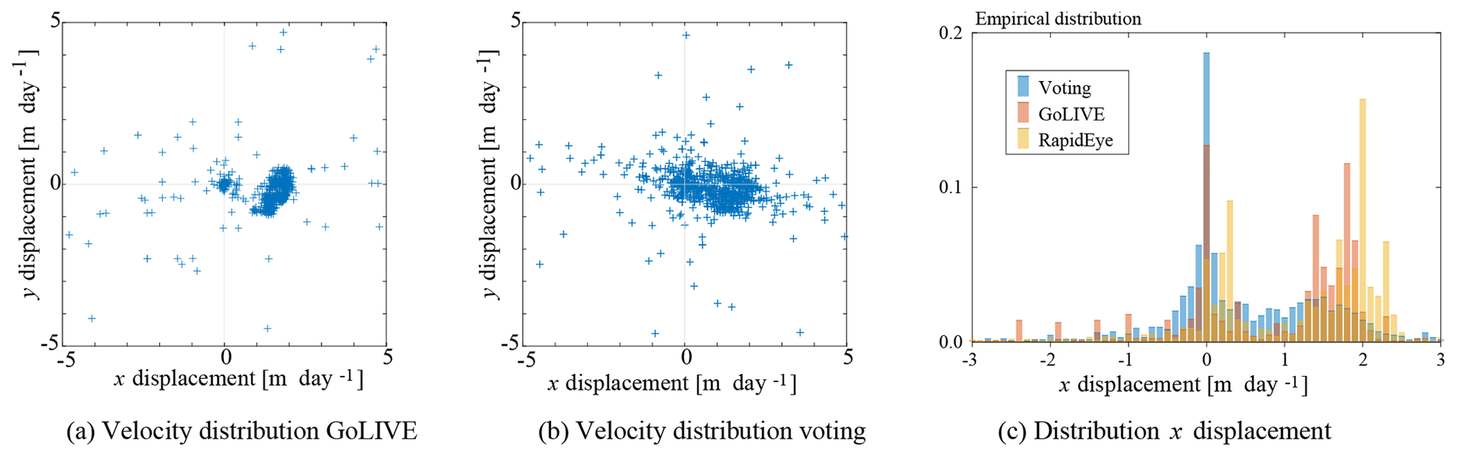
To better assess these results, the distribution of both two-dimensional displacement fields is illustrated in Fig. 10a and b. Two groups of displacement regimes are clearly visible, a cluster showing little movement and a group of displacements with a dominant movement eastwards. The voted distribution has more spread, and outliers are present, but in general the mapping has the correct direction and magnitude. When the x-component of these displacements is compared against the RapidEye displacements, the median of this difference is 0.45 m day⁻¹ for the voting and 0.27 m day⁻¹ for the good GoLIVE pair. A similar trend can be seen in Fig. 10c, which again shows the distributions are similar. The illustrated validations do show the voting scheme is able to capture the general trend of the short-term glacier flow through a large stack of corrupted velocity fields. While the voted estimate is worse than the clean GoLIVE estimate, we stress that the chosen GoLIVE dataset is one clean example within a large collection of partly corrupted displacement fields. Hence it is a step towards efficient information extraction, though the implemented voting has many potential areas for improvement.

4.4 Glaciological observations

When looking at the spatiotemporal dataset some patterns that have been observed by others also appear in our dataset. For example, the full extent of Bering Glacier slows down, as highlighted by Burgess et al. (2012); however our time series covers a period when the full deceleration towards a quiescent state can be seen. This observation of a slowdown can also be made for Donjek Glacier (Abe et al., 2016) and Logan Glacier (Abe and Furuya, 2015); see supplementary video. In the time period covered by our study some surges appear to be initiated. For example, our dataset captures a surge traveling along the main trunk of Klutlan Glacier (see Figs. B1 and B2 in the Appendix B).

Figure 11 Snapshots of ice speeds at different time instances from a data compilation for the summer 2016 surge occurring on Klutlan Glacier (for location see Fig. 7). The used GoLIVE data configuration is shown in Fig. A1, and the data are from the smoothed dataset.

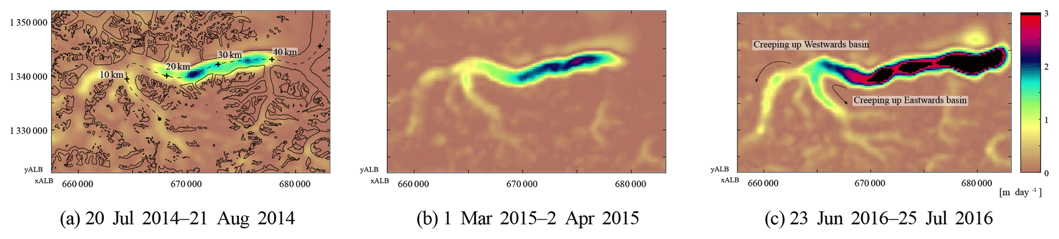
For the surge of Klutlan Glacier, the dataset shows the evolution of its dynamics, as can be seen by some velocity time stamps in Fig. 11. The surge initiation seems to happen in the central trunk of the glacier, and the surge front progresses downwards from there (with steady bulk velocities of around 4 m day⁻¹). The surge also propagates upwards mainly into the westernmost basin. The eastern basin does increase in speed but to a lesser extent, while the middle basin of this glacier system does not seem to be affected significantly. The up-glacier velocity increase is limited and does not reach the headwalls of any basin. In Landsat imagery of late 2017, there is no indication of any heavily crevassed terrain in the upper parts of these basins, which supports the hypothesis of a partially developed surge.

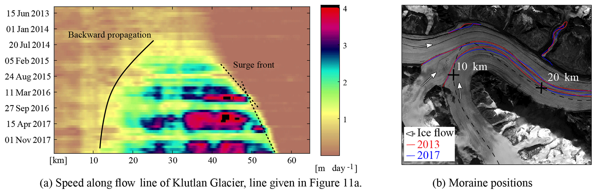
Figure 12 The speed over the central flow line of Klutlan Glacier. The markings of this flow line are shown in panel (a). In panel (b) the convergence of different basins of the Klutlan Glacier is shown; data are from a RapidEye acquisition on 5 September 2013 and 23 September 2017. For comparison the 2013 image is overlain with the two moraine positions.

When looking at the velocities over the flow line of the Klutlan Glacier, as in Fig. 12a, both the extension downstream as well as the upstream progression of the surge can be seen. Most clearly, the surge front seems to propagate downwards with a steady velocity but appears to slow down around the 50 km mark (see dashed line in Fig. 12a), as shown by the break in slope. Here, the glacier widens into a lobe at the terminus. This can suggest ice thickness is homogeneous here or ice thickness does not seem to play an important role in surge propagation.

At the end of the summer of 2016 the tributary just north of the 20 km mark of Klutlan Glacier seems to increase in speed. This can be confirmed by tracing the extent of the looped moraines, as in Fig. 12b. In the same imagery the medial moraines of the meeting point of all basins are mapped as well. Here, the moraine bands before and after the event align well at the junction, indicating a steady or similar contribution over the full period, or an insignificant effect, as the surge has not been developing into very fast flow. In contrast, the lower part of this glacial trunk has moraine bands that do not align.

The surge behavior we observe for Klutlan Glacier, especially the propagation, can be observed at other glaciers within the study area. For Fisher Glacier, a similar increase in speed is observed within the main trunk that later propagates downstream as well as upstream. This also seems to be the case for Walsh Glacier, where a speed increase in the eastern trunk leads to a surge on the northern trunk and a glacier-wide acceleration. On its way the fast-flowing ice initiates surges in tributaries downflow, but the surge extent also moves upslope and tributaries that were further up-glacier from the initial surge start to speed up. This is also seen for Steele Glacier, which develops a surge and Hodgson Glacier is later entrained into the fast flow as well.

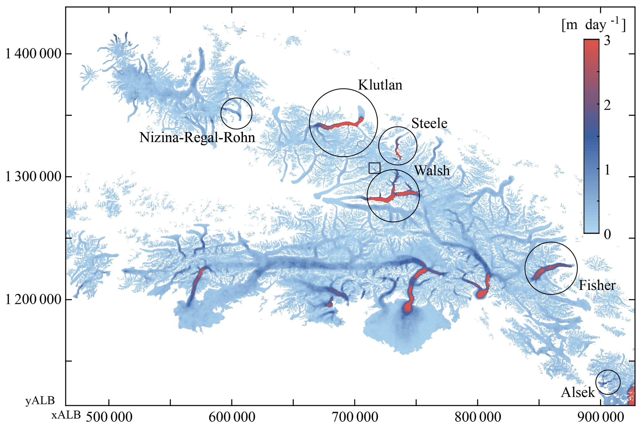
Figure 13 Spread of variation in flow speed (using the difference between the 20th and 80th percentiles) over the observed period (2013–2018). Different dynamic glaciers are encircled, and the square indicates the tributary glacier shown in Fig. C1.

These events are best observed with the help of an animation (see Supplement) but the initial identification was performed through a simple visualization of the spread of flow speed (see Fig. 13). Here the surging glaciers stand out, as do most of the tidewater glaciers, which have a highly dynamic nature at their fronts. Dynamics in smaller tributaries are visible as well; for example, a tributary of the Chitina Glacier seems to have pushed itself into the main trunk within a 2-year time period; see Fig. C1 in Appendix C.

5 Discussion

Synthesized velocity time series estimated from our post-processing chain of GoLIVE image-pair velocity determinations are dependent on the number and distribution of measured displacements (see Appendix A). It may be possible to improve these time series in several ways. Surface features imaged in the same season have similar appearances, allowing good displacement fields to be produced from images which are a year apart, as is typical working practice (Heid and Kääb, 2012b; Dehecq et al., 2015). Annual displacements fields could be helpful when areas are cloud covered for long periods, as these estimates can function as gap fillers in the least-squares estimation. Because the adjustment model assigns equal weighting to individual displacements if no other information is available, some velocity changes might be missed or blurred in time. Such a drawback might be overcome with spatial constraints, such as an advection pattern imposed on the data, although this would increase the amount of post-processing.

Another limitation of our method concerns the glacier kinematics that are constrained by our model. In the current implementation the deviation (σ) is dependent on the time interval. From a measurement perspective this makes sense, but the model does not inherently account for speed change. For long time intervals the fuzzy function forces the deviation to become small. This reduces the ability to obtain a correct match when glacier-dynamics changes are occurring. It might be helpful to explore the improvement when a fixed deviation is set instead. In addition, low scores over glaciated terrain might indicate that the deviation of the displacement is set too tight. When this deviation is given higher bounds, the score increases, and such behavior can then be used as a meaningful measure.

The smoothing parameter used is a single global parameter that assumes isotropy. In order to fulfill this property the spatiotemporal data have been scaled accordingly. However, when severe data gaps are present, the velocity dataset still shows jumps. This will improve when more data are available, for example by including Sentinel-2 data or incorporating across-track matching (Altena and Kääb, 2017a). An increase in votes will result in a better population of the vote space, as can be seen in Fig. 6. In addition, the voting score, that is, the consensus score in the Hough space, can be used as the initial weighting for the smoothing procedure (w in Eq. 2). This might reduce the number of iterations used by the robust smoother. Improvement can be made to the smoother, as our initial implementation has a simple neighborhood function and has no knowledge of glacier-specific properties.

The input data have some possibility of systematic effects that propagate into the synthesized velocity time series. PyCORR-generated displacement is based upon pattern matching methods applied to optical images. Normalized cross-correlation is most sensitive to large intensity variations within the image chips (Debella-Gilo and Kääb, 2011; Fahnestock et al., 2016). Thus specifically for glacierized regions, a low solar illumination angle in winter can cause the pattern matching to fix on shadow edges. Similarly, snow cover and melt-out edges (which occur in autumn and spring) can cause false correlations due to strong contrast in the image chips. To reduce these effects the GoLIVE correlator uses high-pass-filtered imagery (Scambos et al., 1992). Setting the scale of the filter is a subtle trade-off, as shading and shadowing of smaller surface topography are correlatable features and are particularly useful in low-sun-angle conditions (e.g., late fall–winter–early spring). In high-radiometry satellite instruments such as Landsat 8 (and 9), Sentinel 2, and WorldView, information is present in the imagery over shadow cast terrain (Kääb et al., 2016). Hence, in principle, frequency-based orientation correlation (Heid and Kääb, 2012a) might perform better for this specific issue.

6 Conclusions

In 5 years the increase in the number of high-quality optical satellite systems has made it possible to extract detailed and frequent velocity fields over glaciers, ice caps and ice sheets. The GoLIVE dataset is a repository of such velocity fields derived from Landsat 8, available at low latency for analysis by the community. Discovery and exploration of this resource can be complicated due to its vast and growing volume and the complexity of spatiotemporal changes of glacier flow fields. In this study we introduce an efficient post-processing scheme to combine ice velocity data from different overlapping time spans. The presented methodology is resistant to multiple outliers, as voting is used instead of testing. However, since cloud cover or changes in surface characteristics can hamper velocity estimation and spatial flow relations are not incorporated, the resulting synthesized time series still have gaps or outliers. We use a data-driven spatiotemporal smoother to address this issue and enhance the visualization of real glacier flow changes.

Our synthesized time series has a monthly (32 days) temporal interval and 300 m spatial resolution. The time series spans 2013 to 2018 and covers the Saint Elias Mountains and vicinity. Within this study area, we identify several surges of different glaciers at different times and their development over time can be observed. Such details can even be extracted for small tributary glaciers. More surprisingly, velocities for the snow-covered upper glacier areas are, in general, estimated accurately. Thus our synthesized time series can provide an overview of where and when interesting glacier dynamics are occurring.

This study is a demonstration of the capabilities of the new GoLIVE-type remote-sensing products combined with an advanced data filtering and interpolation scheme. We demonstrate that our method can be implemented with ease for a large region, covering several mountain ranges. The derived smoothed time series data contain many subtle additional changes that could be investigated. If this time series is combined with digital elevation model (DEM) time series (Wang and Kääb, 2015), it becomes possible to look at changes in ice mass in great detail.

The presented velocity time series has a high temporal dimension, especially with respect to the sensor 16-day orbit repeat cycle. Though temporal or spatial data gaps are still present (due to the short temporal interval, cloud cover or visual coherence loss) this might partly be addressed by enlarging the temporal resolution or through additional data, such as from Sentinel-2 (Altena and Kääb, 2017a). Fortunately, harmonization with other velocity datasets can be easily implemented because our procedure uses only geometric information and is not dependent on sensor type. With our framework it is thus possible to make a consistent time series composed of a patchwork of optical or SAR remote-sensing products.

Appendix A: Velocity pairs used

The GoLIVE velocity fields used in this study are numerous. In order to obtain an overview of the data used, the velocity pairs are plotted as a network of edges through time, in Fig. A1. Every red arch corresponds to a displacement estimate over a certain period, with a specific footprint (a given path–row combination; see Fig. 1 for localization). The general statistics of the collection of used GoLIVE displacement pairs are given in the Table A1.

Figure A1 Node network of the velocity fields used in this study, a total of 2736 velocity fields. The gray bars span the time interval used for the generation of the different velocity products used in the figures in the main text. The specific numbering is given by their annotation, which is also in gray.

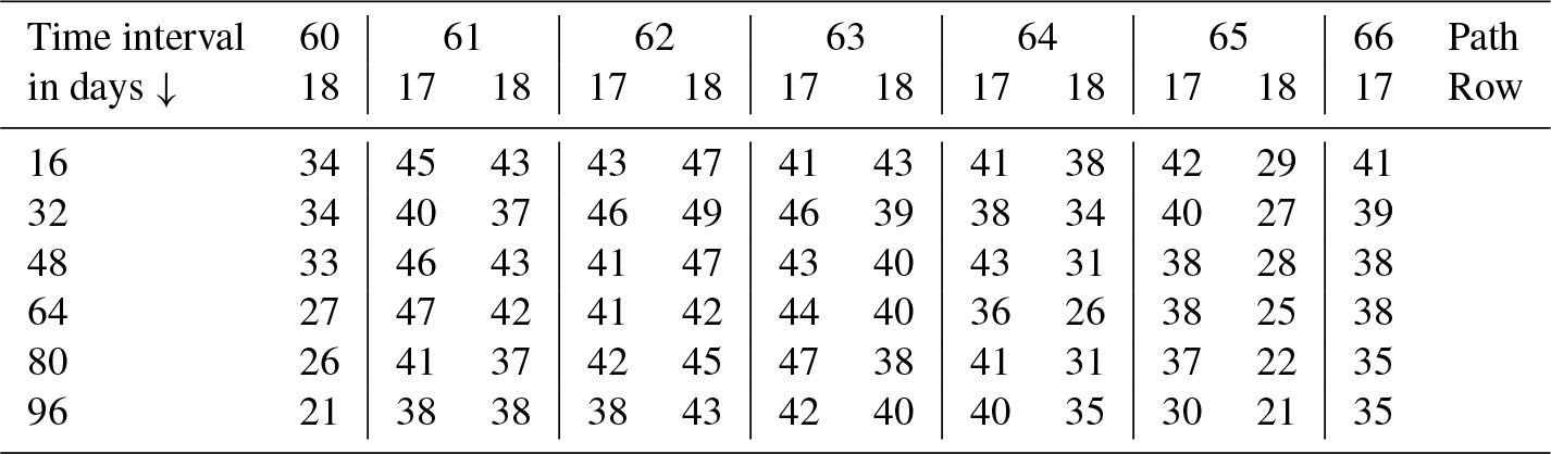
Table A1 Number of GoLIVE displacement products used in the generation of the product, ordered by location through path, row and by relative time interval.

Appendix B: Corrections performed by smoothing

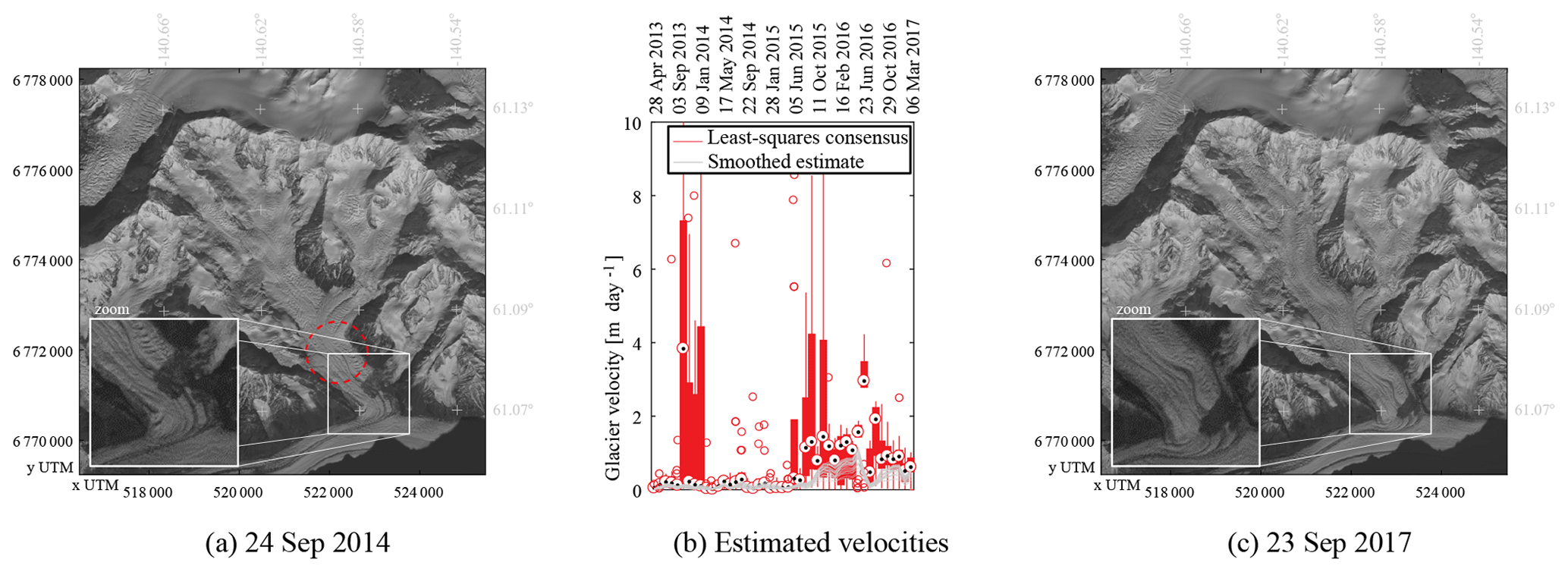
In the following section plots are given of speed variations over selected areas of interest; the locations are denoted in Fig. 11a by black crosses. Every plot has a box plot with the least-squares estimate of a selection of observations. This selection was made through consensus, by voting as described in the paper. The gray lines indicate the smoothed spatiotemporal velocity. These are multiple lines, as not one estimate is used, but a surrounding area of a 5×5 pixel wide neighborhood is taken. This is carried out in order to have sufficient data points and see the spread of the observations and the influence of the smoother. A comparison between both estimated and smoothed versions is shown in the right graph of each figure, where the white line indicates the 1:1.

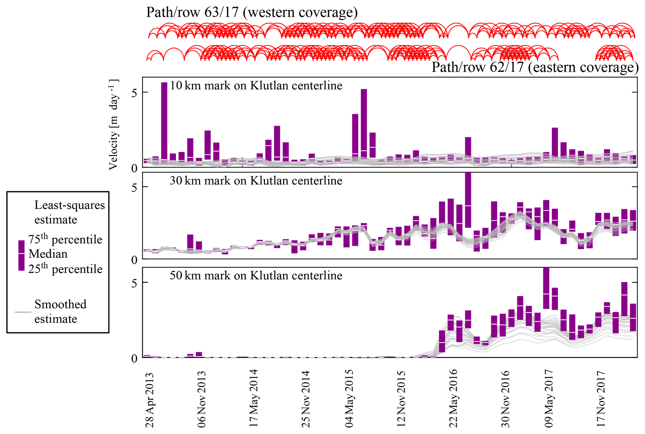
Figure B1 Temporal evolution of three locations along the flow line of Klutlan Glacier. The data from the specific marker and its direct neighborhood are shown. In purple is the box plot of these data while in gray the smoothed estimates are plotted. For the location of the reference marks, please see Fig. 11a. Above the figures, the network configuration of the GoLIVE data for the two covering Landsat scenes is given.

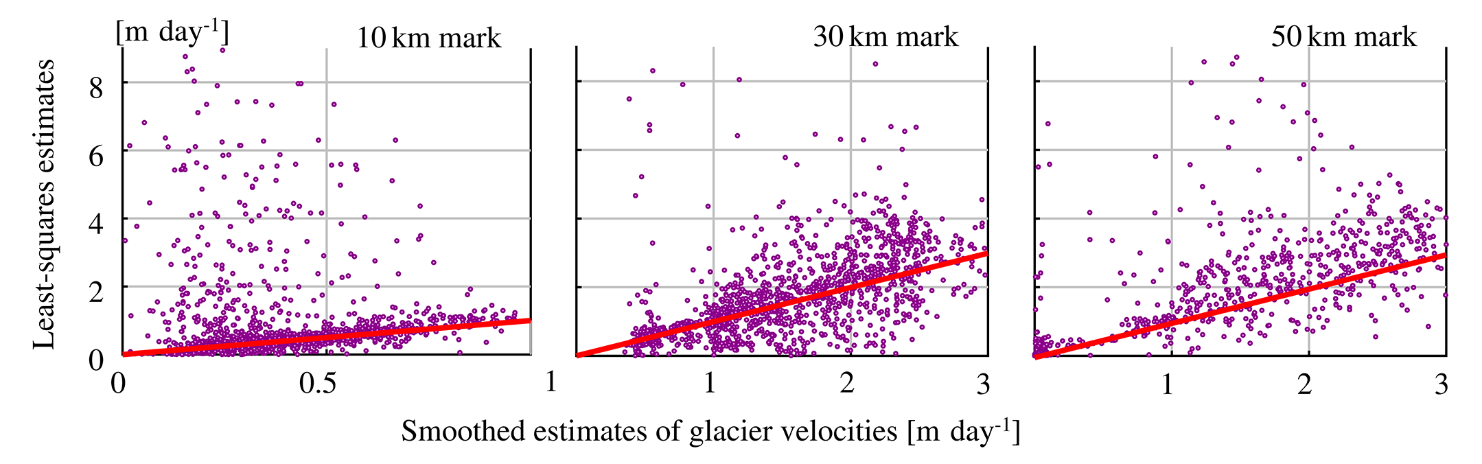
Figure B2 The temporal data shown in Fig. B1 are combined and the least-squares consensus is plotted against the smoothed estimate. The slanted line in all figures corresponds to the 1:1 line.

Figure B3 shows the velocity evolution of the ocean-terminating part of Hubbard Glacier (see Fig. 7 for specific localization). This glacier is seen from paths 61 and 62 and is in row 18. Data come from the GoLIVE dataset and an open configuration is used for the estimation of the velocity. Aliasing occurs in both the slow-moving part (0–4 km) and the fast-moving part (5–7 km). The availability of displacement data from GoLIVE is highest in the winter, as can be seen in Fig. A1. Late in 2015 the Hubbard Glacier seems to slow down completely. However, at the same period the number of GoLIVE displacement data is relatively sparse. When a lack of data occurs, it is very difficult to establish consensus and extract information. To some degree this seems to occur for other years in autumn as well.

Figure B3 (a) Landsat 8 acquisition on 5 September 2013 over Hubbard Glacier; in red is the centerline used for the sampling which is plotted in panels (b) and (c). (b) Velocity estimates using the data of displacements that had consensus during the voting step. (c) Smoothed estimate of velocity evolution over time, using spatial and temporal data and assisted by an off-glacier mask.

Appendix C: Tributary dynamics

From the constructed multi-temporal time series the variance of a low and high quantile can be estimated. This gives an overview of ice masses with a highly dynamic nature. Through this simple analysis, an unknown tributary surge was identified. The push of this tributary into the medial moraine and its velocity record over time can be seen in Fig. C1.

Figure C1 A tributary of Chitina Glacier surged in the period 2015–2016. Images are both acquired by Landsat 8; its location is indicated by a square in Fig. 13. The location of the time series in panel (b) is indicated by a red dashed circle in panel (a).