Arctic sea-ice-free season projected to extend into autumn

The recent Arctic sea ice reduction comes with an increase in the ice-free season duration, with comparable contributions of earlier ice retreat and later advance. CMIP5 models all project that the trend towards later advance should progressively exceed and ultimately double the trend towards earlier retreat, causing the ice-free season to shift into autumn. We show that such a shift is a basic feature of the thermodynamic response of seasonal ice to warming. The detailed analysis of an idealised thermodynamic ice–ocean model stresses the role of two seasonal amplifying feedbacks. The summer feedback generates a 1.6-day-later advance in response to a 1-day-earlier retreat. The underlying physics are the property of the upper ocean to absorb solar radiation more efficiently than it can release heat right before ice advance. The winter feedback is comparatively weak, prompting a 0.3-day-earlier retreat in response to a 1-day shift towards later advance. This is because a shorter growth season implies thinner ice, which subsequently melts away faster. However, the winter feedback is dampened by the relatively long ice growth period and by the inverse relationship between ice growth rate and thickness. At inter-annual timescales, the thermodynamic response of ice seasonality to warming is obscured by inter-annual variability. Nevertheless, in the long term, because all feedback mechanisms relate to basic and stable elements of the Arctic climate system, there is little inter-model uncertainty on the projected long-term shift into autumn of the ice-free season.

1 Introduction

Arctic sea ice has strikingly declined in coverage (Cavalieri and Parkinson, 2012), thickness (Kwok and Rothrock, 2009; Renner et al., 2014; Lindsay and Schweiger, 2015) and age (Maslanik et al., 2011) over the last 4 decades. CMIP5 global climate and Earth system models simulate and project this decline to continue over the 21st century (Massonnet et al., 2012; Stroeve et al., 2012) due to anthropogenic CO₂ emissions (Notz and Stroeve, 2016), with a loss of multi-year ice estimated for 2040–2060 (Massonnet et al., 2012), in the case of a business-as-usual emission scenario.

Less Arctic sea ice also implies changes in ice seasonality, which are important to investigate because of socio-economic (e.g. on shipping; Smith and Stephenson, 2013) and ecosystem implications. Indeed, the length of the Arctic sea ice season exerts a first-order control on the light reaching phytoplankton (Arrigo and van Dijken, 2011; Wassmann and Reigstad, 2011; Assmy et al., 2017) and is crucial to some marine mammals, such as walruses (Laidre et al., 2015) and polar bears (Stern and Laidre, 2016), who use sea ice as a living platform.

Various seasonality diagnostics are discussed in the sea ice literature and definitions as well as approaches vary among authors. The open-water season duration can be diagnosed from satellite ice concentration fields, either as the number of ice-free days (Parkinson, 2014) or as the time elapsed between ice retreat and advance dates, corresponding to the day of the year when ice concentration exceeds or falls under a given threshold (Stammerjohn et al., 2012; Stroeve et al., 2016). The different definitions of the length of the open-water season can differ in subtleties of the computations (notably filtering) and may not always entirely be consistent and comparable. In addition, the melt season duration, distinct from the open-water season duration, has also been analysed from changes in passive microwave emission signals due to the transition from a dry to a wet surface during melting (Markus et al., 2009; Stroeve et al., 2014).

As for changes in the Arctic open-water season duration, satellite-based studies indicate an increase by >5 days per decade over 1979–2013 (Parkinson, 2014) due to earlier ice retreat and later advance (Stammerjohn et al., 2012; Stroeve et al., 2016). There are regional deviations in the contributions to a longer open-water season duration, most remarkably in the Chukchi and Beaufort seas where later ice advance takes over (Johnson and Eicken, 2016; Serreze et al., 2016), which has been attributed to increased oceanic heat advection from the Bering Strait (Serreze et al., 2016). Such changes in the seasonality of Arctic ice-covered waters reflect the response of the surface energy budget to warming. Indeed, warming and ice thinning imply earlier surface melt onset and ice retreat (Markus et al., 2009; Stammerjohn et al., 2012; Blanchard-Wrigglesworth et al., 2010). In addition, a shift towards later ice advance, tightly co-located with earlier retreat, is observed, especially where negative sea ice trends are large (Stammerjohn et al., 2012; Stroeve et al., 2016). This has been attributed to the ice–albedo feedback, namely to the combined action of (i) earlier ice retreat, implying lower surface albedo, and (ii) higher annual solar radiation uptake by the ocean. Such a mechanism (Stammerjohn et al., 2012) explains the ongoing delay in ice advance of a few days per decade from the estimated increase in solar absorption (Perovich et al., 2007), in accord with the observed in situ increase in the annual sea surface temperature (SST) maximum (Steele et al., 2008; Steele and Dickinson, 2016).

The observed increase in the ice-free season duration should continue over the next century, as projected by the CESM Large Ensemble (Barnhart et al., 2016), but this signal is obscured by important levels of internal variability. Other CMIP5 ESMs likely project a longer ice-free season as well, and this is true in the Alaskan Arctic where they have been analysed (Wang and Overland, 2015). In both these studies, the simulated future increases in the ice-free season duration are dominated by the later ice advance. Such behaviour remains unexplained and should be investigated with a larger set of models and regions.

In the present study, we aim at better quantifying the potential changes in Arctic sea ice seasonality and understanding the associated mechanisms. We first revisit the ongoing changes in Arctic sea ice retreat and advance dates using satellite passive microwave records, at both inter-annual and multi-decadal timescales. We also analyse, for the first time over the entire Arctic, all CMIP5 historical and RCP8.5 simulations covering 1900–2300 and study mechanisms at play using a one-dimensional ice–ocean model.

2 Methods

We analyse the recent past and future of sea ice seasonality by computing a series of diagnostics based on satellite observations, Earth system models and a simple ice–ocean model.

2.1 Data sources

Passive microwave sea ice concentration (SIC) retrievals, namely the GSFC Bootstrap SMMR-SSM/I quasi-daily time series product, over 1980–2015 (Comiso, 2000, updated 2015), are used as an observational basis. We also use the CMIP5 Earth system model historical simulations and future projections of SIC. Because of high inter-annual variability in ice advance and retreat dates and because some models lose multi-year ice only late into the 21st century, we retain the nine ESM simulations that pursue RCP8.5 until 2300 (first ensemble member, Table 1). Analysis focuses on 1900–2200, combining historical (1900–2005) and RCP8.5 (2005–2200) simulations. The year 2200 corresponds to the typical date of year-round Arctic sea ice disappearance (Hezel et al., 2014). We also extracted the daily SST output from IPSL-CM5A-LR. All model outputs were interpolated on a 1^∘ geographic grid.

Table 1 Linear trends in ice retreat and advance dates over 2000–2200 (200 years), and long-term ice advance amplification ratios for the individual and mean CMIP5 models and for the 1-D model. Trends and ratios are given as median ± interquartile range over the seasonal ice zone in which trends are significant at a 95 % confidence level (p=0.05). n/a: not applicable.

To investigate how mean state biases may affect ESM simulations, we also included in our analysis a 1958–2015 forced-atmosphere ISPL-CM simulation, i.e. an ice–ocean simulation that was performed with the NEMO-LIM 3.6 model (Rousset et al., 2015), driven by the DFS5 atmospheric forcing (Dussin et al., 2016). NEMO-LIM 3.6 is similar to the ice–ocean component of IPSL-CM5A-LR, except that (i) horizontal resolution is twice as high (1^∘ with refinement near the poles and the equator), (ii) the sea ice model has been upgraded to multiple categories, among other differences, and (iii) a weak sea surface salinity restoration is applied. Such a simulation not only performs generally better than a free-atmosphere ESM run in terms of seasonal ice extent (Fig. S1 in the Supplement; Uotila et al., 2017), but also has year-to-year variations in phase with observations, a feature that is intrinsically not captured in a coupled ESM. However, a caveat of forced-atmosphere simulations is the absence of feedback from the sea ice–ocean surface state onto atmospheric conditions, which can affect the processes that drive changes in ice advance and retreat timing.

2.2 Ice seasonality diagnostics

We use slightly updated computation methods for ice retreat (d_r) and advance (d_a) dates, compared with previous contributions (Parkinson, 1994; Stammerjohn et al., 2012; Stroeve et al., 2016). Ice retreat date (d_r) is defined as the first day of the year when SIC drops below 15 %, whereas ice advance date (d_a) is the first day of the year when SIC exceeds this threshold (Stroeve et al., 2016). The choice of the SIC threshold has no significant impact on the results. All previous studies recognise that a typical 5-day temporal filtering on the input ice concentration is required to get rid of short-term dynamical events (Stammerjohn et al., 2012; Stroeve et al., 2016). By contrast, we use 15 days, in order to get rid of most short-term dynamical ice events, which barely affects trends in d_r and d_a (see Table S1). Another important issue is the reference time axis, which varies among authors. To circumvent the effect of the d_a discontinuity between 31 December and 1 January, we define the origin of time on 1 January and count d_a negatively if it falls between 1 July and 31 December. A safe limit is 1 July because there is no instance of ice advance date between early June and late July in the satellite record or in CMIP5 simulations. The length of the ice-free season is defined as the period during which SIC is lower than 15 %.

The same seasonality diagnostics are computed from model outputs. Yet, since the long-term ESM simulations used here only have monthly SIC outputs, we compute the ice seasonality diagnostics based on monthly SIC fields linearly interpolated daily. Such operation drastically reduces error dispersion but introduces a small systematic bias on d_r (early bias) and d_a (late bias), on the order of 5±5 (6) days. These biases were determined from an analogous processing of satellite records. Dates of ice retreat and advance were derived from a daily interpolation of monthly averaged concentration fields and subsequently compared to direct retrievals based on daily resolved concentration fields (see Fig. S2). The identified biases apply to CMIP5 records because errors stem from the processing of data and do not depend on the type of data used (satellite or CMIP5). These small systematic biases in model ice retreat and advance dates likely contribute to the mean model bias compared to satellite data (Table 1, Fig. 1) but remain small compared to the long-term signals analysed throughout this paper.

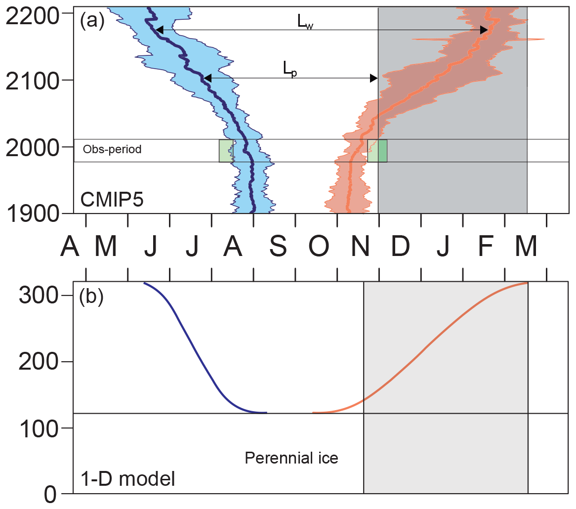
Figure 1 Evolution of the ice seasonality diagnostics (ice retreat date, blue; ice advance date, orange): (a) CMIP5 median and interquartile range, with corresponding range of satellite-derived values (green rectangles 1980–2015) over the 70–80^∘ N latitude band; (b) one-dimensional ice–ocean model results. The ice-free period (L_w), the photoperiod (L_p) and the average polar night (grey rectangle) are also depicted. Note that the systematic difference between observations and CMIP5 models is reduced when accounting for the systematic bias due to the daily interpolation of monthly means in CMIP5 models (see Sect. 2 and Table S2).

The ice seasonality diagnostics and their spatial distribution are reasonably well captured by the mean of selected CMIP5 models over the recent past (Fig. 2). The spatial distribution of ice seasonality diagnostics varies among models, reflecting a possible dependence on the mean state or differences in the treatment of ice dynamics. Larger errors in some individual models (Fig. S3) are associated with an inaccurate position of the ice edge. Overall, ESMs tend to have a shorter open-water season than observed (Figs. 2a–c and S3), which is visible in the North Atlantic and North Pacific regions and can be related to the systematic bias due to the use of interpolated monthly data, but also to the tendency of our model subset to overestimate sea ice. Such an interpretation is supported by (i) the visibly better consistency of the simulated ice seasonality diagnostics with observations in the forced-atmosphere ISPL-CM simulation than in IPSL-CM5A-LR and (ii) by the fact that models with simulated ice extent rather close to observations over the recent past (CESM, CNRM or MPI; Massonnet et al., 2012) are more in line with observed seasonality diagnostics than the other models (Figs. 2 and S3).

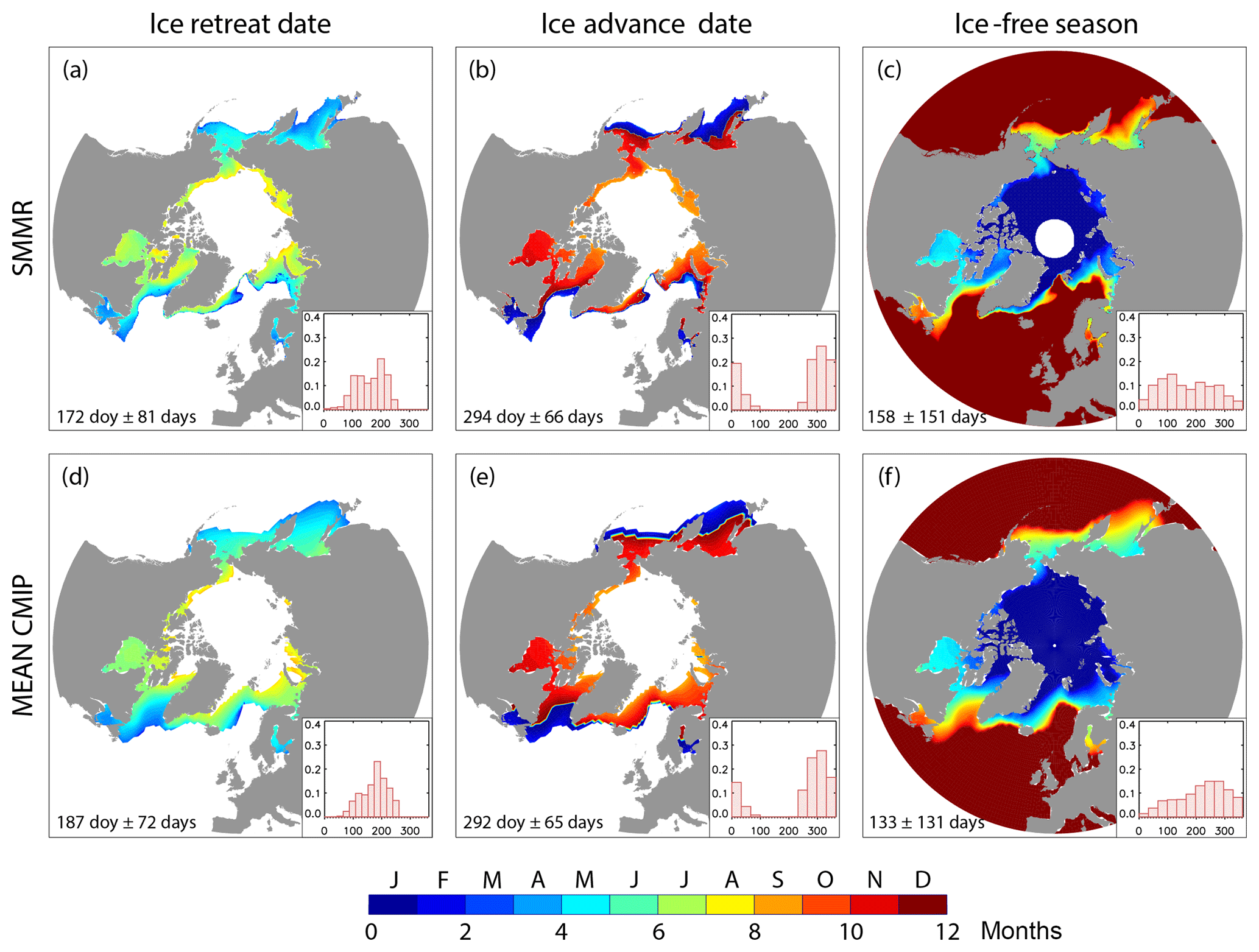
Figure 2 Maps and frequency histograms of (a, d) ice retreat date, (b, e) ice advance date and (c, f) ice-free season length over 1980–2015 (36 years), based on (a, b, c) passive microwave satellite concentration retrievals (Comiso, 2000; updated 2015) and (d, e, f) daily concentration fields averaged over CMIP5 models. Median ± IQR (interquartile range) refers to all points in the seasonal ice zone. See Fig. S3 for individual models.

2.3 Trends in ice advance and retreat dates and related diagnostics

Trends in ice retreat and advance dates were calculated for each satellite or model pixel, from the slope of a least-square fit over a given period, using years when both d_r and d_a are defined. If the number of years used for calculation of the trend is less than one-third of the considered period, a missing value is assigned. One-third compromises between spatial and temporal coverage of the considered time series (see Table S1).

To describe the relative contribution of ice advance and retreat dates to changes in open-water season duration, we introduce a first diagnostic, termed the long-term ice advance vs. retreat amplification coefficient ($R_{\mathrm{a}/\mathrm{r}}^{\text{long}}$). $R_{\mathrm{a}/\mathrm{r}}^{\text{long}}$ is defined as minus the ratio of trends in ice advance to trends in ice retreat dates. The sign choice for $R_{\mathrm{a}/\mathrm{r}}^{\text{long}}$ is such that positive values arise for concomitant long-term trends toward later ice advance and earlier retreat. $R_{\mathrm{a}/\mathrm{r}}^{\text{long}}$ gives synthetic information about trends in ice advance and retreat dates within a single diagnostic. For example, $R_{\mathrm{a}/\mathrm{r}}^{\text{long}}>\mathrm{0}$ means that a trend towards earlier retreat (d_r<0) occurs concurrently with a trend towards later advance (d_a>0). Strictly speaking $R_{\mathrm{a}/\mathrm{r}}^{\text{long}}>\mathrm{0}$ could also indicate later retreat and earlier advance (i.e. a reduction of open-water season duration), which does not happen in a warming climate. Moreover, by definition, $R_{\mathrm{a}/\mathrm{r}}^{\text{long}}>\mathrm{1}$ if the long-term trend in ice advance date exceeds the long-term trend in retreat date in a particular pixel, otherwise $R_{\mathrm{a}/\mathrm{r}}^{\text{long}}<\mathrm{1}$. Note that for $R_{\mathrm{a}/\mathrm{r}}^{\text{long}}$ to be meaningful, we restrict computations to pixels in which trends in both d_r and d_a are significant at a specified confidence level. p=0.05; i.e. a 95 % confidence interval gives the most robust value but heavily restricts the spatial coverage, especially for CMIP5 outputs. By contrast, p=0.25; i.e. a 75 % confidence interval slightly expands coverage but loses some robustness.

In order to study the shorter-term association between retreat and ice advance, we introduce a second diagnostic, termed the short-term ice advance vs. retreat amplification coefficient ($R_{\mathrm{a}/\mathrm{r}}^{\text{short}}$). $R_{\mathrm{a}/\mathrm{r}}^{\text{short}}$ is defined by applying the same reasoning to inter-annual timescales, i.e. minus the linear regression coefficient between detrended ice advance and retreat dates. $R_{\mathrm{a}/\mathrm{r}}^{\text{short}}$ gives information on how anomalies in ice advance date scale with respect to anomalies in retreat dates over the same year, regardless of the long-term trend. Such a definition warrants comparable interpretation for $R_{\mathrm{a}/\mathrm{r}}^{\text{short}}$ and $R_{\mathrm{a}/\mathrm{r}}^{\text{long}}$. In a warming climate, $R_{\mathrm{a}/\mathrm{r}}^{\text{short}}>\mathrm{0}$ indicates concomitant anomalies towards earlier retreat and later advance, and $R_{\mathrm{a}/\mathrm{r}}^{\text{short}}>\mathrm{1}$ indicates that anomalies in advance date are larger than in retreat date.

For computations of $R_{\mathrm{a}/\mathrm{r}}^{\text{long}}$ and $R_{\mathrm{a}/\mathrm{r}}^{\text{short}}$ we use a reference period of 36 years. The length of the available observation period is 36 years and is close to the standard 30 years used in climate sciences. On one occasion (Table 1), we use 200 years as a reference period. The total number of years we can use to qualify changes is 200 years and is the most representative of a long climate change simulation.

All trends and ice advance vs. retreat amplification coefficients given in the rest of the text are the median (± inter-quartile range), taken over the seasonal ice zone. We use non-parametric statistics because the distributions are not Gaussian.

2.4 1-D model

We use the Semtner (1976) zero-layer approach for ice growth and melt above an upper oceanic layer taking up heat, whereas snow is neglected. The model simplifies reality by assuming constant mixed-layer depth, no horizontal advection in ice and ocean, no heat exchange with the interior ocean, and no sensible heat storage in the snow–ice system. The ice–ocean seasonal energetic cycle is computed over 300 years, using climatological solar, latent, and sensible heat fluxes and increasing downwelling long-wave radiation, to represent the greenhouse effect. Ice retreat and advance dates are diagnosed from model outputs (see Appendix A for details). We argue that the Semtner (1976) zero-layer approach is appropriate to study the response of CMIP5 models to warming, as the CMIP5 models with more complicated thermodynamics cannot be distinguished from those using the Semtner zero-layer approach (Massonnet et al., 2018). The zero-layer approach is known to alter the sea ice seasonal cycle (Semtner, 1984), but should not fundamentally affect the processes discussed here.

3 Link between earlier ice retreat and later ice advance in observations and models

3.1 Trends in ice advance and retreat date in observations and models

Over 1980–2015, the ice-free season duration has increased by 9.8±12.1 days decade⁻¹, with nearly equal contributions of earlier ice retreat ($-\mathrm{4.8}\pm \mathrm{7.7}$ days decade⁻¹) and later ice advance (4.9±5.8 days decade⁻¹, median based on satellite observation, updated figures; see Table S1). Variability is high however. Significant trends in both d_r and d_a at the 95 % confidence level are found over a relatively small fraction (22 %) of the seasonal ice zone (Fig. 3), independently of the details of the computation (Table S1). The patterns of changes are regionally contrasted, and Chukchi Sea is the most notable exception to the rule, where later ice advance clearly dominates changes in the ice-free season (Serreze et al., 2016, Fig. 3).

Figure 3 Maps and frequency histograms of linear trends (for hatched zones only) in (a, d) ice retreat date (b, e), ice advance date and (c, f) ice-free season length over 1980–2015 (36 years), based on (a, b, c) passive microwave satellite concentration retrievals (Comiso, 2000; updated 2015); (d, e, f) the mean CMIP5 models. Hatching refers to the 95 % confidence interval (p=0.05). Median ± IQR refers to significant pixels with at least one-third of the years with defined retreat and ice advance dates. See Fig. S4 for individual models.

Trends simulated by the mean of selected CMIP5 models are comparable with observations, in terms of ice retreat date ($-\mathrm{4.4}\pm \mathrm{3.5}$ days decade⁻¹), ice advance date (5.9±3.3 days decade⁻¹) and ice-free season duration (10.3±6.3 days decade⁻¹, Fig. 3). Individual models show larger errors (Fig. S4 to compare with Fig. 3), to be related notably with mean state issues or the spread in the strength of strong oceanic currents, in the North Atlantic and the North Pacific. One common location where trends are underestimated is the North Atlantic region, in particular the Barents Sea, which arguably reflects a weak meridional oceanic heat supply (Serreze et al., 2016). One should be reminded that as reality is a single realisation of internal climate variability (Notz, 2015), a model–observation comparison of this kind is intrinsically limited. This could be of particular relevance in the Barents Sea, which is subject to internally generated decadal-scale variations driven by ocean heat transport anomalies (Yeager et al., 2015).

3.2 Earlier sea ice retreat implies later ice advance

In terms of mean state and contemporary trends, models seem realistic enough for an analysis of changes at pan-Arctic scales but might be less meaningful at regional scales. We first study the contemporary link between earlier retreat and ice advance by looking at the sign of R_a∕r values in contemporary observations and models. Because $R_{\mathrm{a}/\mathrm{r}}^{\text{long}}$ is a ratio of significant trends, and because all models have regional differences as to where trends are significant, we base our analysis on individual models.

Based on observations (Fig. 4), we find positive values of $R_{\mathrm{a}/\mathrm{r}}^{\text{long}}$ in more than 99 % of grid points in the studied zone, provided that computations are restricted where trends on ice retreat and advance dates are significant at a 95 % level (N=5257). In a warming climate, positive $R_{\mathrm{a}/\mathrm{r}}^{\text{long}}$ values mean concomitant and significant trends towards earlier retreat and later advance, whereas missing values reflect either that the trends are not significant or that the point is out of the seasonal ice zone. $R_{\mathrm{a}/\mathrm{r}}^{\text{short}}$ (Fig. 6) is generally smaller (0.21±0.27) than $R_{\mathrm{a}/\mathrm{r}}^{\text{long}}$ (0.71±0.42, 95 % confidence level), and also positive in most pixels (87 % of 23 475 pixels).

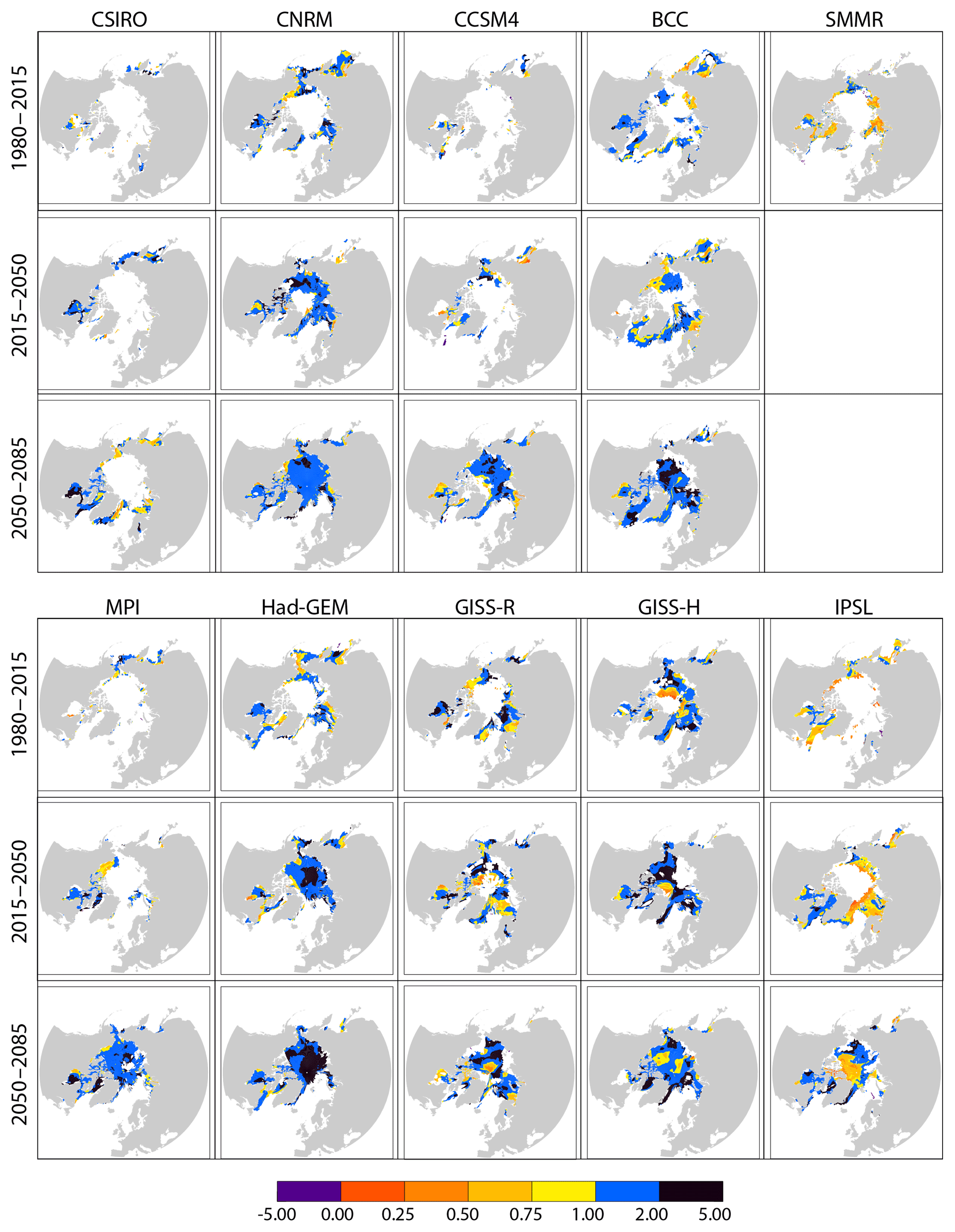
Figure 4 Long-term ice advance vs. retreat amplification coefficient from passive microwave ice concentration retrievals (SMMR; over 1980–2015), and for all individual models over 1980–2015, 2015–2050 and 2050–2085. We use a 75 % (p=0.25) confidence interval for this specific computation. Similar figures (for SMMR and IPSL_CM5A_LR only) for p=0.05 are available in the Supplement (Fig. S9).

CMIP5 models are consistent with the robust link between earlier ice retreat and later advance dates found in observations (Stammerjohn et al., 2012; Stroeve et al., 2016). More generally, we find a robust link between earlier retreat and later advance in all cases: both R_a∕r values are virtually always positive for short- and long-term computations, from observations and models (Figs. 4, 5) over the three analysed periods (1980–2015 for observations and models, 2015–2050 and 2050–2085 for models only) and regardless of internal variability (Figs. S5 and S6). This finding expands previous findings from satellite observations using detrended time series (Stammerjohn et al., 2012; Serreze et al., 2016; Stern and Laidre, 2016), in particular the clear linear correlation found between detrended ice retreat and ice advance dates (Stroeve et al., 2016). Following these authors, we attribute the strong earlier retreat and later ice advance relationship as a manifestation of the ice–albedo feedback: earlier ice retreat leads to an extra absorption of heat by the upper ocean. This heat must be released back to the atmosphere before the ice can start freezing again, leading to later ice advance. Such a mechanism, also supported by satellite SST analysis in the ice-free season (Steele et al., 2008; Steele and Dickinson, 2016), explains the sign of the changes in ice advance date. However, it does not explain the relatively larger magnitude of the trends in ice advance date compared with trends in ice retreat date, studied in the next section.

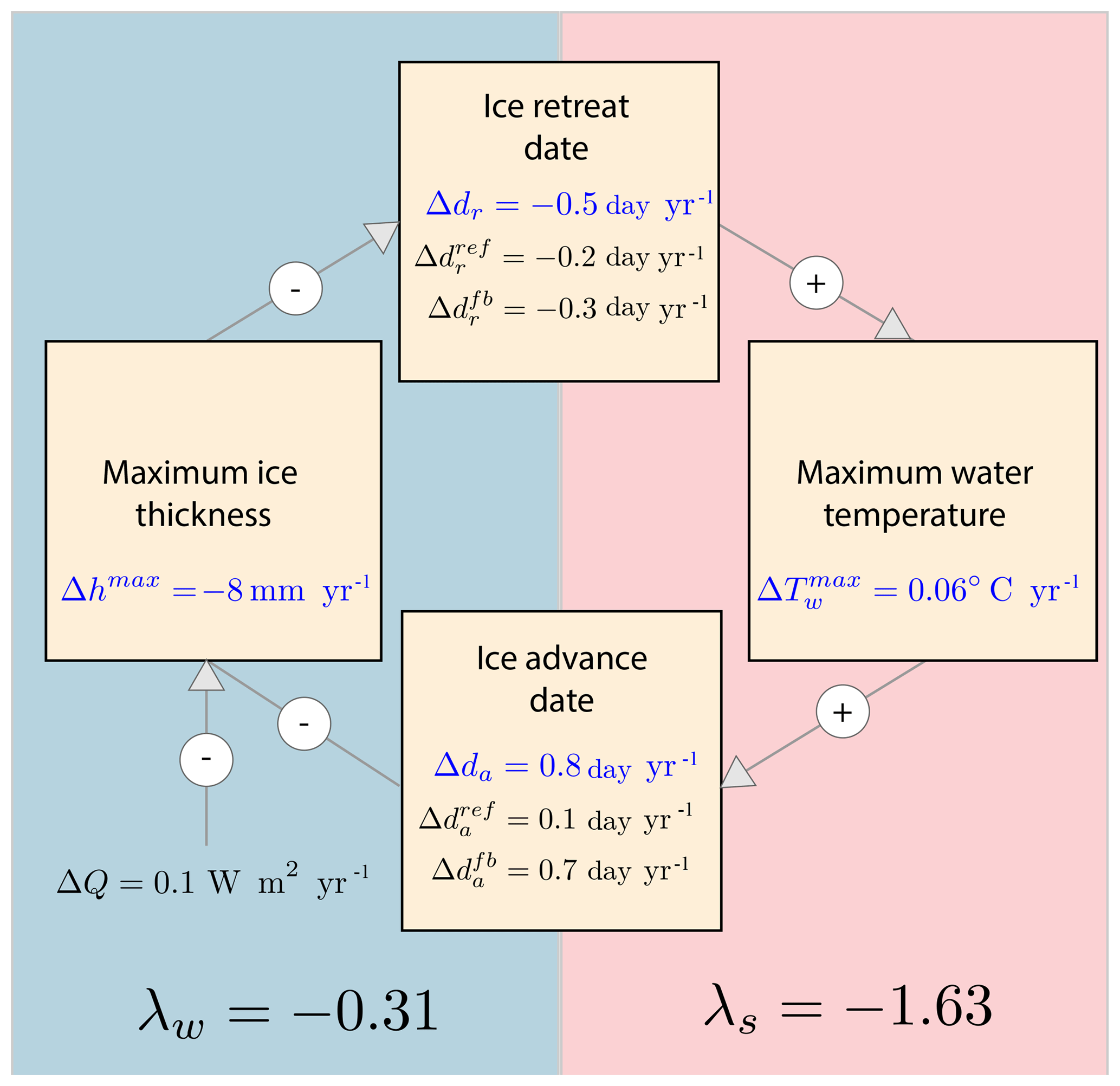
Figure 5 Schematics of the mechanisms shaping the thermodynamic response of sea ice seasonality to a radiative forcing perturbation. The numbers give annual averages simulated by the 1-D model. Changes in ice retreat and advance dates are split between reference (ref) and feedback (fb) responses. See Appendix A for details of the computations.

3.3 Increasingly late ice advance dominates future changes in open-water season

We now focus on the respective contribution of changes in retreat and ice advance dates to the increasingly long open-water season by analysing the magnitude of $R_{\mathrm{a}/\mathrm{r}}^{\text{long}}$. Contemporary values of $R_{\mathrm{a}/\mathrm{r}}^{\text{long}}$ match between model and observations but not spatially (Fig. 4). Over 1980–2015 the simulated $R_{\mathrm{a}/\mathrm{r}}^{\text{long}}$ (CMIP5 mean) is slightly higher (1.1±0.7) than the observational value (0.7±0.4). Since none of the models position the sea ice edge correctly everywhere, it is not surprising that the spatial distribution and the modal $R_{\mathrm{a}/\mathrm{r}}^{\text{long}}$ differ among models and between models and observations. The fact that, by definition, satellite data only sample one realisation of internal variability could contribute to the discrepancy as well. In support of these two arguments, the forced-atmosphere ISPL-CM simulation better simulates the spatial distribution of $R_{\mathrm{a}/\mathrm{r}}^{\text{long}}$ (see Fig. S7), which underlines the role of mean state errors.

As far as future changes are concerned, all models show a qualitatively similar evolution (Figs. 1 and S5). Projected changes in ice retreat and ice advance dates start by approximately 2000 and continue at a nearly constant pace from 2040 until 2200. By 2040, the trend in ice advance date typically becomes larger than the trend in ice retreat date, as indicated by the corresponding mean $R_{\mathrm{a}/\mathrm{r}}^{\text{long}}=\mathrm{1.8}\pm \mathrm{0.4}$ over 2000–2200 (Table 1).

To further understand these contrasting trends between ice retreat and ice advance dates, we mapped $R_{\mathrm{a}/\mathrm{r}}^{\text{long}}$, over 2015–2050 and 2050–2085. We find that, in the course of the 21st century, trends in retreat and ice advance date become significant over increasingly wide regions. The overall $R_{\mathrm{a}/\mathrm{r}}^{\text{long}}$ value increases, as illustrated in Fig. 4. This behaviour is found independent of the considered model and of the internal variability (Figs. S5 and S6).

This finding expands the recent analyses of the CESM Large Ensemble project (Barnhart et al., 2016) and of Alaskan Arctic sea ice in CMIP5 models, finding faster ice coverage decrease in autumn than in spring (Wang and Overland, 2015). Both studies propose that the extra heat uptake in the surface ocean due to an increased open-water season as a potential explanation. As suggested earlier, this indeed explains why $R_{\mathrm{a}/\mathrm{r}}^{\text{long}}$ would be positive but does not explain the amplified delay in ice advance date, that is, why $R_{\mathrm{a}/\mathrm{r}}^{\text{long}}$ would be >1. We are now addressing this question.

3.4 A thermodynamic mechanism for an amplified delay in ice advance date

The reason why $R_{\mathrm{a}/\mathrm{r}}^{\text{long}}$ becomes >1 by 2040 is related to the asymmetric response of ice–ocean thermodynamics to warming: the upper ocean absorbs solar radiation about twice as efficiently as it can release heat right before ice advance. That summer feedback processes dominate is enabled by a relatively weak winter feedback (between later ice advance and earlier retreat the next year).

To come to this statement, we would need diagnostics unavailable in CMIP5, in particular a daily description of the surface energy budget. This is why we used a 1-D thermodynamic model of sea ice growth and melt in relation with the upper-ocean energy budget (Semtner, 1976) to study the idealised thermodynamic response of seasonal ice to a radiative forcing perturbation. Without any particular tuning, the 1-D model simulations feature an evolution that is similar to the long-term behaviour of CMIP5 models (Fig. 1b), with trends in ice advance date (8.2 days decade⁻¹) of larger absolute magnitude than trends in retreat date (−4.7 days decade⁻¹), giving a corresponding value of $R_{\mathrm{a}/\mathrm{r}}^{\text{long}}=\mathrm{1.9}$. All figures fall within the CMIP5 envelope (Table 1).

As explained above, the seasonal relationships between ice advance and retreat dates are underpinned by atmosphere–ice–ocean feedbacks. The non-radiative feedback framework of Goosse et al. (2018; see Appendix A for details) clarifies the study of these relationships. Changes in dates of ice retreat (Δd_r) and advance (Δd_a) in response to a radiative forcing perturbation are split into reference and feedback response terms:

$$\begin{array}{}\text{(1)}& {\displaystyle }\left\{\begin{array}{l}\mathrm{\Delta }{d}_{\text{r}}=\mathrm{\Delta }{d}_{\text{r}}^{\text{ref}}-{\mathit{\lambda }}_{\text{w}}\mathrm{\Delta }{d}_{\text{a}},\\ \mathrm{\Delta }{d}_{\text{a}}=\mathrm{\Delta }{d}_{\text{a}}^{\text{ref}}-{\mathit{\lambda }}_{\text{s}}\mathrm{\Delta }{d}_{\text{r}}.\end{array}\right.\end{array}$$

The sign convention for the feedback terms is such that the link between earlier retreat (Δd_r<0) and later advance (Δd_a>0) gives positive feedback factors. The feedback response refers to the change in d_r (resp. d_a) that can solely be attributed to the change in d_a (resp. d_r). It is expressed using a feedback factor λ_w (resp. λ_s) related to winter (resp. summer) feedback processes. The reference response $\mathrm{\Delta }{d}_{\text{r}}^{\text{ref}}$ (resp. $\mathrm{\Delta }{d}_{\text{a}}^{\text{ref}})$ is that of a virtual system in which the feedback would be absent. Expressions for the reference and feedback response terms, as well as for feedback factors, stem from physical analysis, detailed in Appendix A.

According to this analysis, feedbacks between the dates of retreat and advance dominate the thermodynamic response of ice seasonality (Fig. 5): the reference response to the applied perturbation of 0.1 W m⁻² yr⁻¹ is −0.2 day yr⁻¹ of earlier retreat and 0.1 d yr⁻¹ of later advance.

Ice growth and melt processes generate a relatively weak winter amplifying feedback of ice advance date onto ice retreat date: a shorter growth season implies thinner ice, which subsequently melts away faster. The winter feedback factor is (see Appendix A for derivation)

$$\begin{array}{}\text{(2)}& {\displaystyle }{\mathit{\lambda }}_{\text{w}}={\displaystyle \frac{\mathrm{1}}{\mathrm{2}}}\cdot \left({\displaystyle \frac{d_{\text{r}}-d_{\text{h}}}{d_{\text{h}}-d_{\text{a}}}}\right),\end{array}$$

where d_h is the date of maximum ice thickness, and is solely a function of the ice growth and melt seasonal parameters. λ_w has a rather stable value of 0.31±0.04 over the 127 years of simulated seasonal ice. This value of λ_w indicates a feedback response in ice retreat date of about one-third of the change towards later ice advance the previous autumn. λ_w is <1 for two reasons. First the melt season is shorter than the growth season (Perovich et al., 2003); hence changes in ice advance date translate into weaker changes in ice retreat date. Second, the ice growth rate is larger for thin than for thick ice (Maykut, 1986); hence the maximum winter ice thickness does not decrease due to later advance as much as if the growth rate was constant.

Energetics of the summer ice-free ocean generate a summer amplifying feedback of ice retreat date onto ice advance date, much stronger than the winter feedback. The summer feedback factor is (see Appendix A for derivation)

$$\begin{array}{}\text{(3)}& {\displaystyle }{\mathit{\lambda }}_{\text{s}}=-{\displaystyle \frac{Q_{+}}{Q_{-}}},\end{array}$$

where 〈Q₊〉 and 〈Q₋〉 are the average net positive (negative) atmosphere-to-ocean heat fluxes during the ice-free period. The 1-D model diagnostics give an average value of 1.63±0.18 for λ_s, meaning that earlier retreat implies a feedback delay in ice advance of ∼1.6 times the initial change in ice retreat date. Physically, the strength of the summer feedback is in direct relation with the ice-free upper-ocean energy budget and the evolution of SST. 〈Q₊〉 mostly corresponds to net solar flux, typically 150 W m⁻², and is typically larger than 〈Q₋〉, which corresponds to the net non-solar, mostly long-wave heat flux, at freezing temperatures, typically 75–150 W m⁻² (see Appendix B). Hence, after ice retreat, the SST rapidly increases due to solar absorption into the mixed layer and then decreases much slower until freezing, due to non-solar ocean-to-atmosphere fluxes (Fig. 7a), an evolution that is similar to a recent satellite-based analysis (Steele and Dickinson, 2016). In other words, the energy excess associated with later retreat, stored into the surface ocean, takes extra time to be released before ice advance.

Figure 6 Short-term ice advance vs. retreat amplification coefficient from passive microwave ice concentration retrievals (SMMR; over 1980–2015), and for all individual models over 1980–2015, 2015–2050 and 2050–2085.

Figure 7 (a) Energetics of ice retreat and advance in the simple model: net atmospheric (solid) and solar (yellow) heat fluxes to the ocean; SST (dash), depicted for years 150 and 210. (b) Annual evolution of the simulated sea surface temperature, averaged over the seasonal ice zone, for 2 decades of reference (2015–2025, 2075–2085) as simulated by the IPSL_CM5A_LR model and showing the same temporal asymmetry as in the simple model.

In practise, keeping only the dominant term, $R_{\mathrm{a}/\mathrm{r}}^{\text{long}}$ (the seasonality of the system) reduces to the summer feedback factor:

$$\begin{array}{}\text{(4)}& {\displaystyle }{R}_{\mathrm{a}/\mathrm{r}}^{\text{long}}\approx {\mathit{\lambda }}_{\text{s}}.\end{array}$$

$R_{\mathrm{a}/\mathrm{r}}^{\text{long}}$ appears to vary little among CMIP5 models and even with the 1-D model. Why this could be the case is because the winter and summer feedback factors are controlled by very basic physical processes of the Arctic ice–ocean–climate system and therefore feature relatively low uncertainty levels. Celestial mechanics, ubiquitous clouds and near-freezing temperatures provide strong constraints on the surface radiation balance and hence on the summer feedback factor, that all models likely capture. All models also include the growth and melt season asymmetry and the growth–thickness relationship (see Massonnet et al., 2018) at the source of the relatively weak winter feedback. In IPSL-CM5A-LR, the sole model for which we could retrieve daily SST (Fig. 7b), the evolution of the summer SST in seasonally ice-free regions features a rapid initial increase followed by slow decrease, an indication that the mechanism we propose is sensible.

3.5 Inter-annual variability and extra processes add to the purely thermodynamic response

The CMIP5 response of ice seasonality differs from the idealised thermodynamic response in two notable ways. First, $R_{\mathrm{a}/\mathrm{r}}^{\text{long}}>\mathrm{1}$ only clearly emerges by 2040 in CMIP5 models. Second, $R_{\mathrm{a}/\mathrm{r}}^{\text{long}}$ is typically <1 over the recent past (1980–2015) from the satellite record (Fig. 4). This must be due to the contribution of processes absent from the 1-D model.

As to why the 1-D response would emerge in the course of this century, there are a series of potential reasons that we cannot disentangle with the limited available CMIP5 outputs. (i) The contribution of the subsurface ocean to the surface energy budget, neglected in the 1-D approach, is likely larger today than in the future Arctic. Over the 21st century, the Arctic stratification increases in CMIP5 models (Vancoppenolle et al., 2013; Steiner et al., 2014), whereas the oceanic heat flux convergence should decrease (Bitz et al., 2005). (ii) The solar contribution to the upper-ocean energy budget is smaller today than in the future, as the date of retreat falls closer to the summer solstice. (iii) The surface energy budget is less spatially coherent today than in the future, when the seasonal ice zone moves northwards. The solar radiation maximum drastically changes over 45 to 65^∘ N but has small spatial variations above the Arctic circle (Peixoto and Oort, 1992). Note that in some specific regions, $R_{\mathrm{a}/\mathrm{r}}^{\text{long}}$ is already >1, in particular in the Chukchi Sea, but this has been associated with the summer oceanic heat transport through the Bering Strait (Serreze et al., 2016), which is a localised event, that does not explain why $R_{\mathrm{a}/\mathrm{r}}^{\text{long}}$ would globally become >1 in the future.

The aforementioned processes, ignored in the 1-D model may explain why $R_{\mathrm{a}/\mathrm{r}}^{\text{long}}>\mathrm{1}$ would emerge by mid-century, but internal variability, also absent in the 1-D model, should also be considered (Barnhart et al., 2016). It is remarkable that $R_{\mathrm{a}/\mathrm{r}}^{\text{short}}$ is <1 from both satellite records and CMIP5 model simulations, for all periods and models considered (Fig. 6). This suggests that the ice advance amplification mechanism is not dominant at inter-annual timescales. Indeed, based on inter-annual satellite time series, the standard deviation of ice retreat (SD = 21.6 days) and advance dates (SD = 14.3 days) is high (Stroeve et al., 2016) and the corresponding trends over 1980–2015 are not significant. Conceivably, atmosphere, ocean and ice horizontal transport, operating at synoptic to inter-annual timescales, obscure the simple thermodynamic relation between the ice retreat and advance dates found in the 1-D model. For instance, the advection of sea ice on waters with a temperature higher than the freezing point would imply earlier ice advance. Altogether, this highlights that the ice advance amplification mechanism is a long-term process and stresses the importance of the considered timescales and period as previous studies have already shown (Parkinson et al., 2014; Barnhart et al., 2016).

4 Summary and discussion

The analysis presented in this paper, focused on changes in sea ice seasonality and the associated driving mechanisms, raised the following new findings.

1. All CMIP5 models consistently project that the trend towards later advance progressively exceeds and ultimately doubles the trend towards earlier retreat over this century, causing the ice-free season to shift into autumn.

2. The long-term shift into autumn of the ice-free season is a basic feature of the thermodynamic response of seasonal ice to warming.

3. The thermodynamic shift into autumn of the ice-free season is caused by the combination of relatively strong summer and relatively weak winter feedback processes.

4. Thermodynamic processes only explain the long-term response of ice seasonality, not the inter-annual variations, nor the delayed emergence of the long-term response, which are both consistently simulated features among CMIP5 models.

A central contribution of this paper is the detailed study of the mechanisms shaping the thermodynamic response of sea ice seasonality to radiative forcing in the Semtner (1976) ice–ocean thermodynamic model, using the non-radiative feedback framework of Goosse et al. (2018). The low seawater albedo as compared with ice and the enhanced solar radiation uptake by the ocean had previously been put forward to explain the increase in the length of the open-water season (Stammerjohn et al., 2012). Our analysis completes this view. Extra solar heat reaching the ocean due to earlier ice retreat is absorbed at a higher rate than it can be released until ice advance. This provides a powerful feedback at the source of the shift into autumn of the open-water season. In addition, the link between later advance and earlier retreat the next spring is weak because of the damping effects of the long ice growth period and of the inverse relationship between growth rate and ice thickness. All of these processes are simple enough to be captured by most of the climate models, which likely explains why the different models are so consistent in terms of future ice seasonality.

The link between earlier ice retreat and later advance is found in both satellite retrievals and climate projections, regardless of the considered period and timescale, expanding findings from previous works (Stammerjohn et al., 2012; Serreze et al., 2016; Stern and Laidre, 2016; Stroeve et al., 2016) and further stressing the important control of thermodynamic processes on sea ice seasonality. Yet, two notable features are in contradiction with the thermodynamic response of seasonal ice to warming. First, the long-term response of ice seasonality to warming only appears by mid-century in CMIP5 simulations, when changes in the ice-free season emerge out of variability (Barnhart et al., 2016). Second, changes in ice retreat date are larger than changes in ice advance date at inter-annual timescales. Transport or coupling processes (involving the atmosphere, sea ice, ocean) are the most likely drivers but their effect could not be formally identified because of the lack of appropriate diagnostics in CMIP5. Such a set-up, with a long-term control by thermodynamic processes, has other analogues in climate change studies (Bony et al., 2004; Kröner et al., 2017; Shepherd, 2014).

As the Arctic sea ice seasonality is a basic trait of the Arctic Ocean, a shift of the Arctic sea-ice free season would also have direct ecosystem and socio-economic impacts. The shift in the sea ice seasonal cycle will progressively break the close association between the ice-free season and the seasonal photoperiod in Arctic waters, a relation that is fundamental to photosynthetic marine organisms existing in the present climate (Arrigo and van Dijken, 2011). Indeed, because the ice advance date is projected to overtake the onset of polar night (Fig. 1), typically by 2050, changes in the photoperiod are at this point solely determined by the ice retreat date, and no more by the advance date. The duration of the sea ice season also restricts the shipping season (Smith and Stephenson, 2013; Melia et al., 2017). The second clear implication of the foreseen shift of the Arctic open-water season is that the Arctic navigability would expand to autumn, well beyond the onset of polar night, supporting the lengthening of the shipping season mostly by later closing dates (Melia et al., 2017).

Better projecting future changes in sea ice and its seasonality is fundamental to our understanding of the future Arctic Ocean. Detailed studies of the drivers of sea ice seasonality, in particular the upper-ocean energy budget, the role of winter and summer feedbacks, and the respective contribution of thermodynamic and dynamic processes, are possible tracks towards reduced uncertainties. Further knowledge can be acquired from observations (e.g. Steele and Dickinson, 2016) and Earth system model analyses, for which the expanded set of ice–ocean diagnostics expected in CMIP6, including daily ice concentration fields (Notz et al., 2016), will prove instrumental.

Appendix A: Upper-ocean energetics and ice seasonality in the 1-D ice–ocean model

To characterise the purely thermodynamic response of seasonal ice to a radiative forcing perturbation, we use the Semtner (1976) zero-layer approach for ice growth and melt above an upper oceanic layer taking up heat. Snow is neglected. The ice model equations for surface temperature (T_su) and ice thickness (h) read

$$\begin{array}{}\text{(A1)}& {\displaystyle }& {\displaystyle }{Q}_{\text{atm}}\left(T_{\text{su}}\right)=Q_{\text{c}}\left(T_{\text{su}}\right),\text{(A2)}& {\displaystyle }& {\displaystyle }\mathit{\rho }L{\displaystyle \frac{\text{d}h}{\text{d}t}}=Q_{\text{atm}}\left(T_{\text{su}}\right)+Q_{\text{w}},\end{array}$$

where $Q_{\text{atm}}=Q_{\mathrm{0}}+Q_{\text{sol}}(\mathrm{1}-{\mathit{\alpha }}_i)-\mathit{ϵ}\mathit{\sigma }{T}_{\text{su}}^{\mathrm{4}}$, with Q₀ the sum of downwelling long-wave, latent and sensible heat fluxes, Q_sol the incoming solar flux, α_i=0.64 the ice albedo, ϵ=0.98 the emissivity, and $\mathit{\sigma }=\mathrm{5.67}\times {\mathrm{10}}^{-\mathrm{8}}$ W m⁻² K⁻⁴ the Stefan–Boltzmann constant. Q_c is the heat conduction flux in the ice (>0 downwards), Q_w is the ocean-to-ice sensible heat flux at the ice base, ρ=900 kg m⁻³ is ice density and L=334 kJ kg⁻¹ is the latent heat of fusion. Once the ice thickness vanishes, the water temperature T_w in a h_w=30 m thick upper-ocean layer follows

$$\begin{array}{ll}{\displaystyle }{\mathit{\rho }}_{\text{w}}& {\displaystyle }{c}_{\text{w}}{\displaystyle \frac{\partial T_{\text{w}}}{\partial t}}{h}_{\text{w}}=Q_{\mathrm{0}}+Q_{\text{sol}}(\mathrm{1}-{\mathit{\alpha }}_{\text{w}})[\mathrm{1}-\text{exp}(-\mathit{\kappa }{h}_{\text{w}}\left)\right]\\ \text{(A3)}& {\displaystyle }& {\displaystyle }-\mathit{ϵ}\mathit{\sigma }{T}_{\text{w}}^{\mathrm{4}}.\end{array}$$

ρ_w=1025 kg m⁻³ is water density, c_w=4000 J kg⁻¹ K⁻¹ is water specific heat and ${\mathit{\kappa }}_{\text{w}}=\mathrm{1}/\mathrm{30}$ m⁻¹ is the solar radiation attenuation coefficient in water. Ice starts forming back once T_w returns to the freezing point $T_{\text{f}}=-\mathrm{1.8}$ ^∘C.

Figure A1 Schematic representation of the analysis framework applied to the 1-D model outputs, illustrating the mechanisms of change in ice seasonality between a reference year (solid line) and a subsequent year (dashed line). Ice appears at the ice advance date (d_a). The ice thickness (h) increases until the date of maximum thickness (d_h), then decreases at an average melt rate 〈m〉. Once the ice thickness vanishes at the ice retreat date d_r, the sea water temperature T_w increases due to incoming heat flux Q₊, until the date of maximum temperature (d_T), and finally decreases due to the heat loss Q₋.

The atmospheric solar (Q_sol) and non-solar (Q₀) heat fluxes are forced using the classical standard monthly mean climatologies, typical of central Arctic conditions (Fletcher, 1965). We impose Q_w=2 W m⁻² following Maykut and Untersteiner (1971). We add a radiative forcing perturbation ΔQ=0.1 W m⁻² to the non-solar flux each year to simulate the greenhouse effect. Ice becomes seasonal after 127 years. The model is run until there is no ice left, which takes 324 years.

The following diagnostics of the ice–ocean seasonality (see Fig. A1) are derived from 1-D model outputs:

• d_r (ice retreat date): the first day with $T_{\text{w}}>T_{\text{f}}=-\mathrm{1.8}$ ^∘C;

• d_a (ice advance date): the last day with $T_{\text{w}}>T_{\text{f}}=-\mathrm{1.8}$ ^∘C.

Two other markers of the ice–ocean seasonality prove useful and were also diagnosed:

• d_T (maximum water temperature date): the last day with Q>0.

• d_h (maximum thickness date): the date of maximum ice thickness.

The simulated trend towards later ice advance is on average 1.9 times the trend towards earlier retreat, a value consistent with the CMIP5 value. An advantage of the 1-D model is that the required diagnostics to investigate the ice seasonality drivers are easily available.

Nevertheless, the response of ice seasonality is not straightforward because there are feedbacks between ice retreat and advance dates. First, later advance delays ice growth, reduces the winter maximum thickness and, in turn, implies earlier retreat. Second, earlier retreat adds extra solar heat to the upper ocean, delaying ice advance. To understand the changes in ice seasonality and attributing their causes, we apply the non-radiative feedback framework introduced by Goosse et al. (2018).

Figure A2 Thermodynamic response of sea ice seasonality to warming in the 1-D model. (a) Evolution over the years of the annual contributors to changes in ice retreat and advance date, as simulated by the 1-D model. The yellow line gives the total response Δd_r (resp. Δd_a) as diagnosed from model output. The blue curve gives the reference response $\mathrm{\Delta }{d}_{\text{r}}^{\text{ref}}$ (resp. $\mathrm{\Delta }{d}_{\text{a}}^{\text{ref}})$ to the radiative forcing perturbation as calculated with Eq. (A11) (resp. A16). The red curve gives the feedback response $\mathrm{\Delta }{d}_{\text{r}}^{\text{fb}}$ (resp. $\mathrm{\Delta }{d}_{\text{a}}^{\text{fb}})$, attributed to the feedback from d_a (resp. d_r), calculated with Eqs. (A9) and (A10) (resp. A13 and A15). The black dashed line testifies that the sum of reference and feedback responses matches the total. (b) Evolution over the years of the simulated freeze-up amplification ratio in the 1-D model. The yellow curve gives the freeze-up amplification R, calculated as the ratio of the total response in d_a (Δd_a) divided by the total response in d_r (Δd_r), as diagnosed from the 1-D model. The blue curve gives the contribution of the reference response to the freeze-up amplification ratio ($\mathrm{\Delta }{d}_{\text{a}}^{\text{ref}}/\mathrm{\Delta }{d}_{\text{r}})$. The red curve gives the contribution of the summer feedbacks ($\mathrm{\Delta }{d}_{\text{a}}^{\text{ref}}/\mathrm{\Delta }{d}_{\text{r}}={\mathit{\lambda }}_{\text{s}})$. The black dashed line testifies that the sum of reference and feedback contributions matches the total.

A1 Analysis framework

We split the changes in ice retreat (Δd_r) and advance (Δd_a) dates in response to a radiative forcing perturbation into reference and feedback contributions (Goosse et al., 2018):

$$\begin{array}{}\text{(A4)}& \left\{\begin{array}{l}\mathrm{\Delta }{d}_{\text{r}}=\mathrm{\Delta }{d}_{\text{r}}^{\text{ref}}-{\mathit{\lambda }}_{\text{w}}\mathrm{\Delta }{d}_{\text{a}},\\ \mathrm{\Delta }{d}_{\text{a}}=\mathrm{\Delta }{d}_{\text{a}}^{\text{ref}}-{\mathit{\lambda }}_{\text{s}}\mathrm{\Delta }{d}_{\text{r}}.\end{array}\right.\end{array}$$

The reference response in ice retreat date to the perturbation ($\mathrm{\Delta }{d}_{\text{r}}^{\text{ref}})$ is defined using a virtual reference system in which winter feedbacks (from d_a onto d_r) would not operate. The feedback response ($\mathrm{\Delta }{d}_{\text{r}}^{\text{fb}})$ is the total minus the reference response and is assumed proportional to the change in ice advance date (Δd_a). Equivalently it is the part of the total change in d_r that can solely be linked to changes in d_a in the previous autumn. The feedback factor λ_w quantifies the strength of this link. The sign convention is such that concomitant later advance (Δd_a>0) and earlier retreat (Δd_r>0) give a positive feedback factor. The definitions for the feedback and reference response terms in ice advance date are similar. The only difference is that the summer feedback factor λ_s quantifies the link between earlier retreat and later advance in the same year.

A2 Winter response

To formulate what determines the changes in ice retreat date, we focus on the ice season (Fig. A1) and use the maximum ice thickness to connect d_a to d_r. The ice thickness increases from zero on d=d_a until a maximum h^max reached when d=d_h. Stefan's law of ice growth (Stefan, 1981) gives

$$\begin{array}{}\text{(A5)}& h^{\text{max}}\approx \sqrt{-{\displaystyle \frac{\mathrm{2}k\langle T_{\text{su}}\rangle }{\mathit{\rho }L}}\cdot \left(d_{\text{h}}-d_{\text{a}}\right)},\end{array}$$

where 〈T_su〉 is the surface temperature averaged over [d_a,d_h], i.e. over the ice growth period. Stefan's law is not exact but precise enough, reproducing the simulated annual values of h^max within 2±2 % of the 1-D model simulation over the 197 years of seasonal ice. The other advantage of Stefan's ice thickness is to be differentiable. Defining $v=k/\left(\mathit{\rho }{\text{Lh}}^{\text{max}}\right)$, the change in ice thickness due to the radiative forcing perturbation is, after linearisation,

$$\begin{array}{}\text{(A6)}& \mathrm{\Delta }{h}^{\text{max}}=v\cdot \langle T_{\text{su}}\rangle \cdot \left[\mathrm{\Delta }{d}_{\text{a}}-\mathrm{\Delta }{d}_{\text{h}}+(d_{\text{a}}-d_{\text{h}}){\displaystyle \frac{\mathrm{\Delta }\langle T_{\text{su}}\rangle }{\langle T_{\text{su}}\rangle }}\right].\end{array}$$

Now, to connect the maximum ice thickness to the ice retreat date, we consider the melt season. The ice melts from h^max on d=d_h until ice thickness vanishes on d=d_r. Hence

$$\begin{array}{}\text{(A7)}& h^{\text{max}}=\langle m\rangle \cdot \left(d_{\text{r}}-d_{\text{h}}\right),\end{array}$$

where 〈m〉 is the average melt rate, assumed to be negative.

We now combine growth and melt seasons and eliminate h^max. Differentiating (Eq. A7), then injecting Δh^max from (Eq. A6) and dividing by 〈m〉, we get

$$\begin{array}{ll}{\displaystyle }& {\displaystyle \frac{\mathrm{\Delta }\langle m\rangle }{\langle m\rangle }}\cdot \left(d_{\text{r}}-d_{\text{h}}\right)+\mathrm{\Delta }{d}_{\text{r}}-\mathrm{\Delta }{d}_{\text{h}}={\displaystyle \frac{v\cdot \langle T_{\text{su}}\rangle }{\langle m\rangle }}\cdot \\ \text{(A8)}& {\displaystyle }& {\displaystyle }\left[\mathrm{\Delta }{d}_{\text{a}}-\mathrm{\Delta }{d}_{\text{h}}+\left(d_{\text{a}}-d_{\text{h}}\right){\displaystyle \frac{\mathrm{\Delta }\langle T_{\text{su}}\rangle }{\langle T_{\text{su}}\rangle }}\right].\end{array}$$

Using Stefan's law (Eq. A5) to replace h^max in the definition of v, the first factor on the right-hand side of Eq. (A8) can be rewritten as

$$\begin{array}{}\text{(A9)}& {\displaystyle \frac{v\cdot \langle T_{\text{su}}\rangle }{\langle m\rangle }}=-{\displaystyle \frac{\mathrm{1}}{\mathrm{2}}}.\left({\displaystyle \frac{d_{\text{r}}-d_{\text{h}}}{d_{\text{h}}-d_{\text{a}}}}\right)\equiv -{\mathit{\lambda }}_{\text{w}}.\end{array}$$

Substituting Eq. (A9) into (A8) and rearranging terms gives the desired decomposition between reference and feedback responses:

$$\begin{array}{}\text{(A10)}& \mathrm{\Delta }{d}_{\text{r}}=\mathrm{\Delta }{d}_{\text{r}}^{\text{ref}}-{\mathit{\lambda }}_{\text{w}}\mathrm{\Delta }{d}_{\text{a}},\end{array}$$

where the reference response gathers all terms independent of Δd_a:

$$\begin{array}{}\text{(A11)}& \mathrm{\Delta }{d}_{\text{r}}^{\text{ref}}=\left(\mathrm{1}-{\mathit{\lambda }}_{\text{w}}\right)\mathrm{\Delta }{d}_{\text{h}}+\left(d_{\text{r}}-d_{\text{h}}\right).\left({\displaystyle \frac{\mathrm{\Delta }\langle T_{\text{su}}\rangle }{\mathrm{2}\langle T_{\text{su}}\rangle }}-{\displaystyle \frac{\mathrm{\Delta }\langle m\rangle }{\langle m\rangle }}\right).\end{array}$$

The terms on the right-hand side reflect the contributions of (i) changes in the date of maximum thickness, (ii) changes in surface temperature and (iii) changes in surface melt rate. The feedback term in (Eq. A10) isolates the contribution of changes in ice advance date and λ_w now clearly appears as a feedback factor. To compute the forced and feedback terms from model output, the annual time series of 〈T_su〉, 〈m〉 and d_h were extracted from model outputs.

The proposed decomposition (Eq. A10) is supported by analysis: the sum of calculated reference and feedback responses (black dashed line in Fig. A2a) matches the total change in ice retreat date as diagnosed from model output (yellow line in Fig. A2a).

A3 Summer forced and feedback responses

The link between ice advance date and the previous ice retreat date stems from the conservation of energy in the ice-free upper ocean. Once ice disappears on d=d_r, the upper ocean takes up energy (see Fig. A1). The surface ocean temperature T_w increases from the freezing point until a maximum, reached on d=d_T. Then the upper ocean starts losing energy and T_w decreases, reaching the freezing point at the date of ice advance d_a. Over this temperature path, the energy gain from d_a to d_T must equal the energy loss from d_T to d_a:

$$\begin{array}{}\text{(A12)}& \langle Q_{+}\rangle \left(d_{\text{T}}-d_{\text{r}}\right)=-\langle Q_{-}\rangle \left(d_{\text{a}}-d_{\text{T}}\right),\end{array}$$

where 〈Q₊〉 is the average net heat flux from the atmosphere to the upper ocean over [d_r,d_T] and 〈Q₋〉 is the average net heat flux over [d_max,d_a]. Defining

$$\begin{array}{}\text{(A13)}& {\displaystyle }{\mathit{\lambda }}_{\text{s}}=-{\displaystyle \frac{\langle Q_{+}\rangle }{\langle Q_{-}\rangle }}\end{array}$$

and rearranging terms in (Eq. A12), we relate d_a to d_r via surface energy fluxes:

$$\begin{array}{}\text{(A14)}& d_{\text{a}}=-{\mathit{\lambda }}_{\text{s}}{d}_{\text{r}}+d_{\text{T}}\left(\mathrm{1}+{\mathit{\lambda }}_{\text{s}}\right).\end{array}$$

By differentiating this expression, we get the sought decomposition between reference and feedback responses:

$$\begin{array}{}\text{(A15)}& \mathrm{\Delta }{d}_{\text{a}}=\mathrm{\Delta }{d}_{\text{a}}^{\text{ref}}-{\mathit{\lambda }}_{\text{s}}\mathrm{\Delta }{d}_{\text{r}}.\end{array}$$

The reference response groups all terms independent of Δd_r:

$$\begin{array}{}\text{(A16)}& \mathrm{\Delta }{d}_{\text{r}}^{\text{ref}}=-d_{\text{r}}\mathrm{\Delta }{\mathit{\lambda }}_{\text{s}}+\mathrm{\Delta }{d}_{\text{T}}+\mathrm{\Delta }\left({\mathit{\lambda }}_{\text{s}}{d}_{\text{T}}\right).\end{array}$$

The terms on the right-hand side reflect the contributions of (i) changes in energy fluxes, (ii) change in the date of maximum water temperature and (iii) non-linearities between both. The feedback term in Eq. (A15) isolates the contribution of changes in ice retreat date and λ_s clearly now appears as a feedback factor. To compute the reference and feedback terms from the 1-D model output, the annual time series of 〈Q₊〉, 〈Q₋〉 and d_T were extracted.

Analysis supports the proposed decomposition: the sum of calculated feedback and reference responses (black dashed curve in Fig. A2a) is equal to the total response diagnosed from model outputs (yellow curve in Fig. A2a).

A4 Analysis

Forced and feedback responses clarify the drivers of the shift into autumn that characterises the thermodynamic response of ice seasonality to the perturbation of the radiative forcing. The response of the system is dominated by changes in ice advance date, which are by far dominated by the feedback response (0.8 d yr⁻¹), much larger than the reference response (0.1 d yr⁻¹; see Fig. A2a). The summer feedback factor λ_s, equal on average to 1.63, largely amplifies changes in retreat date. The positive sign of λ_s indicates that earlier retreat implies later advance. Why λ_s>1 is because positive heat fluxes into the ocean 〈Q₊〉 are typically larger than the heat losses 〈Q₋〉 that follow the ocean temperature maximum. Hence it takes more time for the surface ocean to release the extra energy than it takes to absorb it.

The response of ice retreat date, following winter processes, is characterised by roughly equal contributions of reference (−0.2 d yr⁻¹) and feedback (−0.3 d yr⁻¹) responses. The feedback factor λ_w is equal to 0.31 on average; hence changes in d_a imply changes in d_r of smaller magnitude. The positive sign means that later advance implies earlier retreat. Why λ_w<1 is because of two robust features of the ice seasonal cycle that dampen the impact of changes in d_a on d_r. First the melt season is shorter than the growth season; hence changes in ice advance date translate into weaker changes in ice retreat date. Second, the ice growth rate is larger for thin than for thick ice; hence the maximum winter ice thickness does not decrease due to later advance as much as if the growth rate were constant. (The 1∕h dependence in growth rate explains the extra 0.5 factor in λ_w.)

Now considering the ice advance vs. retreat amplification coefficient, it can be expressed as a function of feedback and reference responses:

$$\begin{array}{}\text{(A17)}& {\displaystyle }R\equiv -{\displaystyle \frac{\mathrm{\Delta }{d}_{\text{a}}}{\mathrm{\Delta }{d}_{\text{r}}}}={\mathit{\lambda }}_{\text{s}}+{\displaystyle \frac{\mathrm{\Delta }{d}_{\text{a}}^{\text{ref}}}{\mathrm{\Delta }{d}_{\text{r}}}}.\end{array}$$

R and its two contributors are depicted in Fig. A2b. Summer feedbacks largely dominate R, such that R≈λ_s is a reasonable approximation.

Let us finally note that both feedback factors are determined by fundamental physical features of ice–ocean interactions, likely going beyond climate uncertainties. The winter feedback is determined by the shape of the seasonal cycle and the non-linear dependence of ice growth rate, which are likely invariant across models. As for the summer feedback, the scaling detailed in Appendix B indicates that the related feedback factor is constrained by celestial mechanics, ubiquitous clouds and near-freezing temperatures. This likely contributes to the low level of uncertainty in R among the different climate models.

Appendix B: Scaling of the ice-free ocean energy budget

The 1-D model results show a direct link between, on the one hand, the ratio of long-term trends in ice advance and retreat date ($R_{\mathrm{a}/\mathrm{r}}^{\text{long}}$) and the energetics of the ice-free ocean on the other hand:

$$\begin{array}{}\text{(B1)}& {\displaystyle }{R}_{\mathrm{a}/\mathrm{r}}^{\text{long}}\approx {\mathit{\lambda }}_{\text{s}}=-\langle Q_{+}\rangle /\langle Q_{-}\rangle ,\end{array}$$

where 〈Q₊〉 and 〈Q₋〉 are the average net positive (negative) atmosphere-to-ocean heat fluxes during the ice free-period. CMIP5 and 1-D model results suggest that over long timescales, this ratio is stable and does not vary much among models, with values ranging from 1.5 to 2. Why this ratio would have so little variability is because celestial mechanics, ubiquitous clouds and near-freezing temperatures provide strong constraints on the radiation balance, which dominates the surface energy budget.

Assuming that non-solar components cancel each other, the mean heat gain is mostly solar:

$$\begin{array}{}\text{(B2)}& {\displaystyle }\langle Q_{+}\rangle =\langle Q_{\text{sol}}\left(\mathrm{1}-{\mathit{\alpha }}_{\text{w}}\right)\left[\mathrm{1}-\text{exp}\left(-\mathit{\kappa }{h}_{\text{w}}\right)\right]{\rangle }_{\text{early\hspace{0.17em}ice-free\hspace{0.17em}season}},\end{array}$$

where the mean is taken over the first part of the ice-free period, typically covering July or June. Of remarkable importance is that the magnitude of clear-sky solar flux above the Arctic Circle deviates by less than 20 W m⁻², both in space and time, around the summer solstice (see, e.g. Peixoto and Oort, 1992). Assuming summer cloud skies would remain the norm, we take 150 W m⁻² as representative for 〈Q₊〉.

The mean heat loss is mostly non-solar:

$$\begin{array}{}\text{(B3)}& {\displaystyle }\langle Q_{-}\rangle =\langle Q_{\text{lw}}-\mathit{ϵ}\mathit{\sigma }{T}_{\text{w}}^{\mathrm{4}}+Q_{\text{sh}}+Q_{\text{lh}}{\rangle }_{\text{late\hspace{0.17em}ice-free\hspace{0.17em}season}},\end{array}$$

and corresponds to the second part of the ice-free period, typically covering August to October. Downwelling long-wave radiation flux Q_lw corresponds to cloud skies at near-freezing temperatures, for which 250 W m⁻² seems reasonable (Persson et al., 2002). The thermal emission would be that of the ocean, a nearly ideal black body, at near-freezing temperatures, and should not depart much from 300 W m⁻². The sensible (Q_sh) and latent (Q_lh) heat fluxes are relatively more uncertain. In current ice-covered conditions, turbulent fluxes imply a net average heat loss, typically smaller than 10 W m⁻² (Persson et al., 2002). Over an ice-free ocean, however, turbulent heat losses would obviously increase, in particular through the latent heat flux, but also become more variable at synoptic timescales. Assuming that turbulent heat fluxes would in the future Arctic compare to what they are today in ice-free ocean regions of the North Pacific, we argue that they would correspond to a 25 W m⁻² heat loss, definitely not exceeding 100 W m⁻² (Yu et al., 2008).

Taken together, these elements give an estimated R value ranging from 1 to 2, for which uncertainties on the dominant radiation terms of the energy budget are small and inter-model differences in turbulent heat fluxes would be decisive in determining the actual value of the ratio.