the Creative Commons Attribution 4.0 License.
the Creative Commons Attribution 4.0 License.
 | 01 Feb 2019
Global glacier volume projections under high-end climate change scenarios
Sarah Shannon
Robin Smith
Andy Wiltshire
Tony Payne
Matthias Huss
Richard Betts
John Caesar
Aris Koutroulis
Darren Jones
Stephan Harrison
The Paris agreement aims to hold global warming to well below 2 ∘C and to pursue efforts to limit it to 1.5 ∘C relative to the pre-industrial period. Recent estimates based on population growth and intended carbon emissions from participant countries suggest global warming may exceed this ambitious target. Here we present glacier volume projections for the end of this century, under a range of high-end climate change scenarios, defined as exceeding +2 ∘C global average warming relative to the pre-industrial period. Glacier volume is modelled by developing an elevation-dependent mass balance model for the Joint UK Land Environment Simulator (JULES). To do this, we modify JULES to include glaciated and unglaciated surfaces that can exist at multiple heights within a single grid box. Present-day mass balance is calibrated by tuning albedo, wind speed, precipitation, and temperature lapse rates to obtain the best agreement with observed mass balance profiles. JULES is forced with an ensemble of six Coupled Model Intercomparison Project Phase 5 (CMIP5) models, which were downscaled using the high-resolution HadGEM3-A atmosphere-only global climate model. The CMIP5 models use the RCP8.5 climate change scenario and were selected on the criteria of passing 2 ∘C global average warming during this century. The ensemble mean volume loss at the end of the century plus or minus 1 standard deviation is % for all glaciers excluding those on the peripheral of the Antarctic ice sheet. The uncertainty in the multi-model mean is rather small and caused by the sensitivity of HadGEM3-A to the boundary conditions supplied by the CMIP5 models. The regions which lose more than 75 % of their initial volume by the end of the century are Alaska, western Canada and the US, Iceland, Scandinavia, the Russian Arctic, central Europe, Caucasus, high-mountain Asia, low latitudes, southern Andes, and New Zealand. The ensemble mean ice loss expressed in sea level equivalent contribution is 215.2±21.3 mm. The largest contributors to sea level rise are Alaska (44.6±1.1 mm), Arctic Canada north and south (34.9±3.0 mm), the Russian Arctic (33.3±4.8 mm), Greenland (20.1±4.4), high-mountain Asia (combined central Asia, South Asia east and west), (18.0±0.8 mm), southern Andes (14.4±0.1 mm), and Svalbard (17.0±4.6 mm). Including parametric uncertainty in the calibrated mass balance parameters gives an upper bound global volume loss of 281.1 mm of sea level equivalent by the end of the century. Such large ice losses will have inevitable consequences for sea level rise and for water supply in glacier-fed river systems.
- Article
(8799 KB) - Full-text XML
-
Supplement
(1385 KB) - BibTeX
- EndNote


Glaciers act as natural reservoirs by storing water in the winter and releasing it during dry periods. This is particularly vital for seasonal water supply in large river systems in South Asia (Immerzeel and Bierkens, 2013; Lutz et al., 2014; Huss and Hock, 2018) and central Asia (Sorg et al., 2012) where glacier melting contributes to streamflow and supplies fresh water to millions of people downstream. Glaciers are also major contributors to sea level rise, despite their mass being much smaller than the Greenland and Antarctic ice sheets (Kaser et al., 2006; Meier et al., 2007; Gardner et al., 2013). Since glaciers are expected to lose mass into the twenty-first century (Radić et al., 2014; Giesen and Oerlemans, 2013; Slangen et al., 2014; Huss and Hock, 2015), there is an urgent need to understand how this will affect seasonal water supply and food security. To study this requires a fully integrated impact model which includes the linkages and interactions among glacier mass balance, river runoff, irrigation, and crop production.
The Joint UK Land Environment Simulator (JULES) (Best et al., 2011) is an appropriate choice for this task because it models these processes, but it is currently missing a representation of glacier ice. JULES is the land surface component of the Met Office global climate model (GCM), which is used for operational weather forecasting and climate modelling studies. JULES was originally developed to model vegetation dynamics and snow and soil hydrological processes within the GCM but now has a crop model to simulate crop yield for wheat, soybean, maize, and rice (Osborne et al., 2014), an irrigation demand scheme to extract water from ground and river stores, and two river routing schemes: Total Runoff Integrating Pathways (Oki et al., 1999) (TRIP) and the RFM kinematic wave model (Bell et al., 2007). The first objective of this study is to add a glacier ice scheme to JULES to contribute to the larger goal of developing a fully integrated impact model.
The second objective is to make projections of glacier volume changes under high-end climate change scenarios, defined as exceeding 2 ∘C global average warming relative to the pre-industrial period (Gohar et al., 2017). The Paris agreement aims to hold global warming to well below 2 ∘C and to pursue efforts to limit it to 1.5 ∘C relative to the pre-industrial period; however, there is some evidence that this target may be exceeded. Revised estimates of population growth suggest there is only a 5 % chance of staying below 2 ∘C and that the likely range of temperature increase will be 2.0–4.9 ∘C (Raftery et al., 2017). A global temperature increase of 2.6–3.1 ∘C has been estimated based on the intended carbon emissions submitted by the participant countries for 2020 (Rogelj et al., 2016). Therefore, in this study we make end-of-the-century glacier volume projections, using a subset of downscaled Coupled Model Intercomparison Project Phase 5 (CMIP5) models which pass 2 and 4 ∘C global average warming. The CMIP5 models use the Representative Concentration Pathways (RCP) RCP8.5 climate change scenario for high greenhouse gas emissions.
The paper is organised as follows: in Sect. 2 we describe the glacier ice scheme implemented in JULES and the procedure for initialising the model. Section 3 describes how glacier mass balance is calibrated and validated for the present day. Section 4 presents future glacier volume projections, a comparison with other studies, and a discussion on parametric uncertainty in the calibration procedure. Section 5 discusses the results, model limitations, and areas for future development. In Sect. 6, we summarise our findings with some concluding remarks.
JULES (described in detail by Best et al., 2011) characterises the land surface in terms of subgrid-scale tiles representing natural vegetation, crops, urban areas, bare soil, lakes, and ice. Each grid box is comprised of fractions of these tiles with the total tile fraction summing to 1. The exception to this is the ice tile, which cannot co-exist with other surface types in a grid box. A grid box is either completely covered in ice or not. All tiles can be assigned elevation offsets from the grid box mean, which is typically set to zero as a default.
To simulate the mass balance of mountain glaciers more accurately we extend the tiling scheme to flexibly model the surface exchange in different elevation classes in each JULES grid box. We have added two new surface types, glaciated and unglaciated elevated tiles, to JULES (version 4.7) to describe the areal extent and variation in height of glaciers in a grid box (Fig. 1). Each of these new types, at each elevation, has its own bedrock subsurface with a fixed heat capacity. These subsurfaces are impervious to water, and have no carbon content, so they have no interaction with the complex hydrology or vegetation found in the rest of JULES. Because glaciated and unglaciated elevated tiles have their own separate bedrock subsurface they are not allowed to share a grid box with any other tiles. For instance, grid boxes cannot contain partial coverage of elevated glacier ice and vegetated tiles.
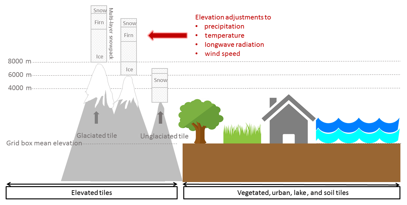
Figure 1Schematic of JULES surface types inside a single grid box. The new elevated glaciated and unglaciated tiles are shown on the left-hand side. Note that elevated glaciated and unglaciated tiles are not allowed to share a grid box with the other tiles.
JULES is modified to enable tile heights to be specified in metres above sea level (m a.s.l.), as opposed to the default option, which is to specify heights as offsets from the grid box mean. This makes it easier to input glacier hypsometry into the model and to compare the output to observations for particular elevation bands. To implement this change, the grid box mean elevation associated with the forcing data is read in as an additional ancillary file. Downscaling of the climate data, described in Sect. 2.1, is calculated using the difference between the elevation band (zband) and the grid box mean elevation (zgbm).
For the purposes of this study JULES is set up with a spatial resolution of 0.5∘ and 46 elevation bands ranging from 0 to 9000 m in increments of 250 m. The horizontal resolution of 0.5∘ is used because it matches the forcing data used to drive the model. The vertical resolution of 250 m was used based on computational cost. The vertical and horizontal resolutions of the model can be modified for any setup.
Each elevated glacier tile has a snowpack which can gain mass through accumulation and freezing of water and lose mass through sublimation and melting. JULES has a full energy balance multilevel snowpack scheme which splits the snowpack into layers, each having a thickness, temperature, density, grain size (used to determine albedo), and solid ice and liquid water contents. The initialisation of the snowpack properties and the distribution of the glacier tiles as a function of height are described in Sect. 2.3. Fresh snow accumulates at the surface of the snowpack at a characteristic low density and compacts towards the bottom of the snowpack under the force of gravity. When rain falls on the snowpack, water is percolated through the layers if the pore space is sufficiently large, while any excess water contributes to the surface runoff. Liquid water below the melting temperature can refreeze. A full energy balance model is used to calculate the energy available for melting. If all the mass in a layer is removed within a model time step then removal takes place in the layer below. The temperature at each snowpack level is calculated by solving a set of tridiagonal equations for heat transfer with the surface boundary temperature set to the air temperature and the bottom boundary temperature set to the subsurface temperature.
A snowpack may exist on both glaciated and unglaciated elevated tiles if there is accumulation of snow. The elevation-dependent mass balance (SMBz,t) is calculated as the change in the snowpack mass (S) between successive time steps.
The scheme assumes that the snowpack can grow or shrink at elevation bands depending on the mass balance, but that tile fraction (derived from the glacier area) is static with time. The ability to grow or shrink the snowpack at elevation levels means that the model includes a simple elevation feedback mechanism. If the snowpack shrinks to zero at an elevation band, then the terminus of the glacier moves to the next level above. Conversely, if the snowpack grows at an elevation band it just continues to grow and there is no process to move the ice from higher elevations to lower elevations. Typically, in an elevation feedback, when a glacier grows the surface of the glacier will experience a cooler temperature; however in this case, the snowpack surface experiences the temperature of the elevation band.
2.1 Downscaling of climate forcing on elevations
Both glaciated and unglaciated elevated tiles are assigned heights in metres above sea level and the following adjustments are made to the surface climate in grid boxes in which glaciers are present.
2.1.1 Air temperature and specific humidity
Temperature is adjusted for elevation using a dry and moist adiabatic lapse rate depending on the dew point temperature. First the elevated temperature follows the dry adiabat:
where T0 is the surface temperature, γdry is the dry adiabatic temperature lapse rate (∘C m−1), and Δz is the height difference between tile elevation and the grid box mean elevation associated with the forcing data.
If Tz is less than the dew point temperature Tdew then the temperature adjustment follows the moist adiabat. A moist adiabatic lapse rate is calculated using the surface specific humidity from the forcing data.
q0 is the surface specific humidity, lc is the latent heat of fusion of water at 0 ∘C (2.501×10⁶ J kg−1), g is the acceleration due to gravity (9.8 m s−2), r is the gas constant for dry air (287.05 kg K−1), R is the ratio of molecular weights of water and dry air (0.62198), and Tv (K) is the virtual dew point temperature.
The height at which the air becomes saturated z is
The elevated temperature following the moist adiabat is then
Additionally, when Tz<Tdew, the specific humidity is adjusted for height. The adjustment is made using the elevated air temperature and surface pressure from the forcing data using a lookup table based on the Goff–Gratch formula (Bakan and Hinzpeter, 1987). The adjusted humidity is then used in the surface exchange calculation.
2.1.2 Longwave radiation
Downward longwave radiation is adjusted by assuming the atmosphere behaves as a black body using Stefan–Boltzmann's law. The radiative air temperature at the surface Trad,0 is calculated using the downward longwave radiation provided by the forcing data LW↓z0
where σ is the Stefan–Boltzmann constant ( W m−2 K−4). The radiative temperature at height is then adjusted:
where T0 is the grid box mean temperature from the forcing data and Tz is the elevated air temperature. This is used to calculate the downward longwave radiation LW↓z at height
An additional correction is made to ensure that the grid box mean downward longwave radiation is preserved:
where frac is the tile fraction.
2.1.3 Precipitation
To account for orographic precipitation, large-scale and convective rainfall and snowfall are adjusted for elevation using an annual mean precipitation gradient (%/100 m):
where P0 is the surface precipitation, γprecip is the precipitation gradient, and z0 is the grid box mean elevation. Rainfall is also converted to snowfall when the elevated air temperature Tz is less than the melting temperature (0 ∘C). The adjusted precipitation fields are input into the snowpack scheme and the hydrology subroutine. When calibrating the present-day mass balance, we needed to lapse rate correct the precipitation to obtain sufficient accumulation in the mass balance compared to observations. The consequence of this is that the grid box mean precipitation is no longer conserved. We tested scaling the precipitation in a way that conserves the grid box mean by reducing the precipitation near the surface and increasing it at height, but this did not yield enough precipitation to obtain a good agreement with the mass balance observations. If the model is being used to simulate river discharge in glaciated catchments, then the precipitation lapse rate could be used as a parameter to calibrate the discharge.
2.1.4 Wind speed
A component of the energy available to melt ice comes from the sensible heat flux, which is related to the temperature difference between the surface and the elevation level and the wind speed. Glaciers often have katabatic (downslope) winds which enhance the sensible heat flux and increase melting (Oerlemans and Grisogono, 2002). It is important to represent the effects of katabatic winds on the mass balance when trying to model glacier melt, particularly at lower elevations where the katabatic wind speed is highest.
To explicitly model katabatic winds would require knowledge of the grid box mean slope at elevation bands, so instead a simple scaling of the surface wind speed is used to represent katabatic winds. Over glaciated grid boxes the wind speed is
where γwind is a wind speed scale factor and u0 is the surface wind speed. The simple scaling increases the wind speed relative to the surface forcing data and assumes that the scaling is constant for all heights. Although our approach is rather crude, we found that scaling the wind speed was necessary to obtain reasonable values for the sensible heat flux. This is seen when we compare the modelled energy balance components to observations from the Pasterze glacier in the Alps (Greuell and Smeets, 2001). The measurements consist of incoming and outgoing short- and longwave radiation, albedo, temperature, wind speed, and roughness length at five heights between 2205 and 3325 m a.s.l. on the glacier. Table S6 in the Supplement lists the observed and modelled energy balance components and meteorological data, for experiments with and without wind speed scaling. The comparison shows that JULES underestimates the sensible heat flux by at least 1 order of magnitude and the modelled wind speed is 4 times lower than the observations. When we increase the wind speed to match the observations there is a better agreement with the observed sensible heat flux. The surface exchange coefficient, which is used to calculate the sensible heat flux, is a function of the wind speed in the model.
2.2 Glacier ice albedo scheme
The existing spectral albedo scheme in JULES simulates the darkening of fresh snow as it undergoes the process of aging (Warren and Wiscombe, 1980). In this scheme the change in albedo as snow ages is related to the growth of the snow grain size, which is a function of the snowpack temperature. The snow aging scheme does not reproduce the low albedo values typically observed on glacier ice; therefore a new albedo scheme is used. The new scheme is a density-dependent parameterisation which was developed for implementation in the Surface Mass Balance and Related Sub-surface processes (SOMARS) model (Greuell and Konzelmann, 1994). The scheme linearly scales the albedo from the value of fresh snow to the value of ice, based on the density of the snowpack surface. The new scheme is used when the surface density of the top 10 cm of the snowpack (ρsurface) is greater than the firn density (550 kg m−3) and the original snow aging scheme is used when (ρsurface) is less than the firn density.
αλ,snow is the maximum albedo of fresh snow, αλ,ice is the albedo of melting ice, ρsnow is the density of fresh snow (250 kg m−3), and ρice is the density of ice (917 kg m−3). The albedo scaling is calculated separately in two radiation bands: visible (VIS) wavelengths λ=0.3–0.7 µm and near-infrared (NIR) wavelengths λ=0.7–5.0 µm. The parameters, αvis,ice, αvis,snow, αnir,ice, αnir,snow, γtemp, γprecip, and γwind are tuned to obtain the best agreement between simulated and observed surface mass balance profiles for the present day (see Sect. 3).
2.3 Initialisation
The model requires initial conditions for (1) the snowpack properties and (2) glaciated and unglaciated elevated tile fractions within a grid box. The location of glacier grid points, the initial tile fraction, and the present-day ice mass are set using data from the Randolph Glacier Inventory version 6 (RGI6) (RGI Consortium, 2017). This dataset contains information on glacier hypsometry and is intended to capture the state of the world's glaciers at the beginning of the twenty-first century. A new feature of the RGI6 is 0.5∘ gridded glacier volume and area datasets, produced at 50 m elevation bands. Volume was constructed for individual glaciers using an inversion technique to estimate ice thickness created using glacier outlines, a digital elevation model, and a technique based on the principles of ice flow mechanics (Farinotti et al., 2009; Huss and Farinotti, 2012). The area and volume of individual glaciers have been aggregated onto 0.5∘ grid boxes. We bin the 50 m area and volume into elevations bands varying from 0 to 9000 m in increments of 250 m to match the elevation bands prescribed in JULES.
2.3.1 Initial tile fraction
The elevated glaciated fraction is
where RGI_area is the area (km2) at height from the RGI6, n is the tile elevation, and gridbox_area (km2) is the area of the grid box. In this configuration of the model, any area that is not glaciated is set to a single unglaciated tile fraction (fracrock) with a grid box mean elevation. It is possible to have an unglaciated tile fraction at every elevation band, but since the glaciated tile fractions do not grow or shrink, we reduce our computation cost by simply putting any unglaciated area into a single tile fraction.
nBands =37 is the number of elevation bands.
2.3.2 Initial snowpack properties
The snowpack is divided into 10 levels in which the top nine levels consist of 5 m of firn snow with depths of 0.05, 0.1, 0.15, 0.2, 0.25, 0.5, 0.75, 1, and 2 m and the bottom level has a variable depth. For each snowpack level the following properties must be set: density (kg m−3), ice content (kg m−2), liquid water content (kg m−2), grain size (µm), and temperature (K). We assume there is no liquid content in the snowpack by setting this to zero. The density at each level is linearly scaled with depth, between the value for fresh snow at the surface (250 kg m−3) and the value for ice at the bottom level (917 kg m−3).
For the future simulations the thickness and ice mass at the bottom of the snowpack come from thickness and volume data in the RGI6. The data are based on thickness inversion calculations from Huss and Farinotti (2012) for individual glaciers which are consolidated onto 0.5∘ grid boxes. The ice mass is calculated from the RGI6 volume assuming an ice density of 917 kg m−3. For the other layers the ice mass is calculated by multiplying the density by the layer thickness, which is prescribed above. For the calibration period, the ice mass at the start of the run (1979) is unknown. In the absence of any information about this, a constant depth of 1000 m is used, which is selected to ensure that the snowpack never completely depletes over the calibration period. This consists of 995 m of ice at the bottom level of the snowpack and 5 m of firn in the layers above. The ice content of the bottom level is the depth (995 m) multiplied by the density of ice.
The snow grain size used to calculate spectral albedo (see Sect. 2.2) is linearly scaled with depth and varies between 50 µm at the surface for fresh snow and 2000 µm at the base for ice. The snowpack temperature profile is calculated by spinning the model up for 10 years for the calibration period and 1 year for the future simulations. The temperature at the top layer of the snowpack is set to the January mean temperature and the bottom layer and subsurface temperature are set to the annual mean temperature. For the calibration period the monthly and annual temperature comes from the last year of the spin-up. Setting the snowpack temperature this way gives a profile of warming towards the bottom of the snowpack representative of geothermal warming from the underlying soil. The initial temperature of the bedrock before the spin-up is set to 0 ∘C but this adjusts to the climate as the model spins up. We use these prescribed snowpack properties as the initial state for the calibration and future runs.
3.1 Model calibration
Elevation-dependent mass balance is calibrated for the present day by tuning seven model parameters and comparing the output to elevation-band specific mass balance observations from the WGMS (2017). Calibrating mass balance against in situ observations is a technique which has been used by other glacier modelling studies (Radić and Hock, 2011; Giesen and Oerlemans, 2013; Marzeion et al., 2012). For the calibration, annual elevation-band mass balance observations are used because there are data available for 16 of the 18 RGI6 regions. For validation, winter and summer elevation-band mass balance is used because there are fewer data available.
The tuneable parameters for mass balance are VIS snow albedo (αvis,snow), VIS melting ice albedo (αvis,ice), NIR snow albedo (αnir,snow), NIR melting ice albedo (αnir,ice), orographic precipitation gradient (γprecip), temperature lapse rate (γtemp), and wind speed scaling factor (γwind).
Random parameter combinations are selected using Latin hypercube sampling (McKay et al., 1979) among plausible ranges which have been derived from various sources outlined below. This technique randomly selects parameter values; however, reflectance in the VIS wavelength is always higher than in the NIR. To ensure the random sampling does not select NIR albedo values that are higher or unrealistically close to the VIS albedo values, we calculate the ratio of VIS to NIR albedo using values compiled by Roesch et al. (2002). The ratio VIS ∕ NIR is calculated as 1.2 so any albedo values that exceed this ratio are excluded from the analysis. This reduces the sample size from 1000 to 198 parameter sets.
In the VIS wavelength the fresh snow albedo is tuned between 0.99 and 0.7 for which an upper bound value comes from observations of very clean snow with few impurities in the Antarctic (Hudson et al., 2006). The lower bound represents contaminated fresh snow and comes from taking approximate values from a study based on laboratory experiments of snow, with a large grain size (110 µm) containing 1680 parts per billion of black carbon (Hadley and Kirchstetter, 2012). VIS snow albedos of approximately 0.7 have also been observed on glaciers with black carbon and mineral dust contaminants in the Tibetan Plateau (Zhang et al., 2017). In the NIR wavelength the fresh snow albedo is tuned between 0.85 and 0.5 for which the upper bound comes from spectral albedo observations made in Antarctica (Reijmer et al., 2001). We use a very low minimum albedo for ice in the VIS and NIR wavelengths (0.1), in order to capture the low reflectance of melting ice.
Table 1Tuneable parameters for mass balance calculation and their ranges from the literature.
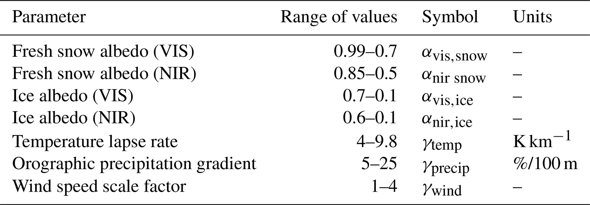
The temperature lapse rate is tuned between values of 4.0 and 10 ∘C km−1 for which the upper limit is determined from physically realistic bounds and the lower limit is from observations based at glaciers in the Alps (Singh, 2001). The temperature lapse rate in JULES is constant throughout the year and assumes that temperature always decreases with height.
The wind speed scaling factor γwind is tuned within the range of 1–4 to account for an increase in wind speed with height and for the presence of katabatic winds. The upper bound is estimated using wind observations made along the profile of the Pasterze glacier in the Alps during a field campaign (Greuell and Smeets, 2001). Table S6 in the Supplement contains the wind speed observations on the Pasterze glacier. The maximum observed wind speed was 4.6 m s−1 (at 2420 m a.s.l.) while the WATCH–ERA Interim dataset (WFDEI) (Weedon et al., 2014) surface wind speed for the same time period was 1.1 m s−1, indicating a scaling factor of approximately 4.
The orographic precipitation gradient γprecip is tuned between 5 and 25 % per 100 m. This parameter is poorly constrained by observations; therefore a large tuneable range is sampled. Tawde et al. (2016) estimated a precipitation gradient of 19 % per 100 m for 12 glaciers in the western Himalayas using a combination of remote sensing and in situ meteorological observations of precipitation. Observations show that the precipitation gradient can be as high as 25 % per 100 m for glaciers in Svalbard (Bruland and Hagen, 2002) while glacier–hydrological modelling studies have used much smaller values of 4.3 % per 100 m (Sorg et al., 2014) and 3 % per 100 m (Marzeion et al. (2012). The tuneable parameters and their minimum and maximum ranges are listed in Table 1.
The model is forced with daily surface pressure, air temperature, downward longwave and shortwave surface radiation, specific humidity, rainfall, snowfall, and wind speed from the WFDEI dataset (Weedon et al., 2014). To reduce the computation time, only grid points at which glacier ice is present are modelled. An ensemble of 198 calibration experiments are run. For each simulation the model is spun up for 10 years and the elevation-dependent mass balance is compared to observations at 149 field sites over the years 1979–2014.
The elevation-dependent mass balance observations come from stake measurements taken every year at different heights along the glaciers. Many of the mass balance observations in the World Glacier Monitoring Service (WGMS, 2017) are supplied without observational dates. In this case, we assume the mass balance year starts on 1 October and ends on 30 September with the summer commencing on 1 May. Dates in the Southern Hemisphere are shifted by 6 months. The observations are grouped according to standardised regions defined by the RGI6 (Fig. 2). The best regional parameter sets are identified by finding the minimum root-mean-square error between the modelled mass balance and the observations.
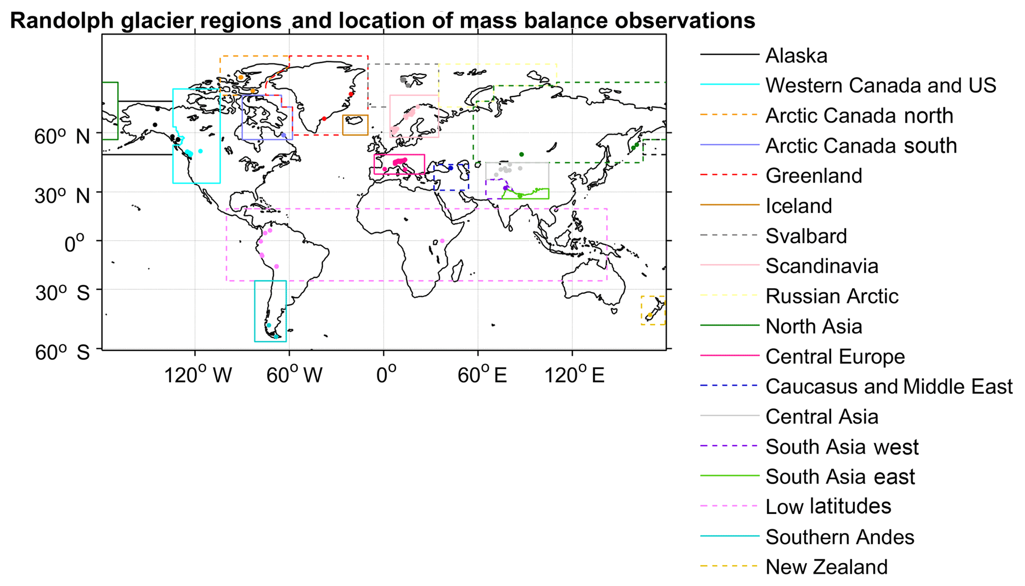
Figure 2The location of mass balance profile observation glaciers from the World Glacier Monitoring Service and the Randolph Glacier Inventory regions (version 6.0).
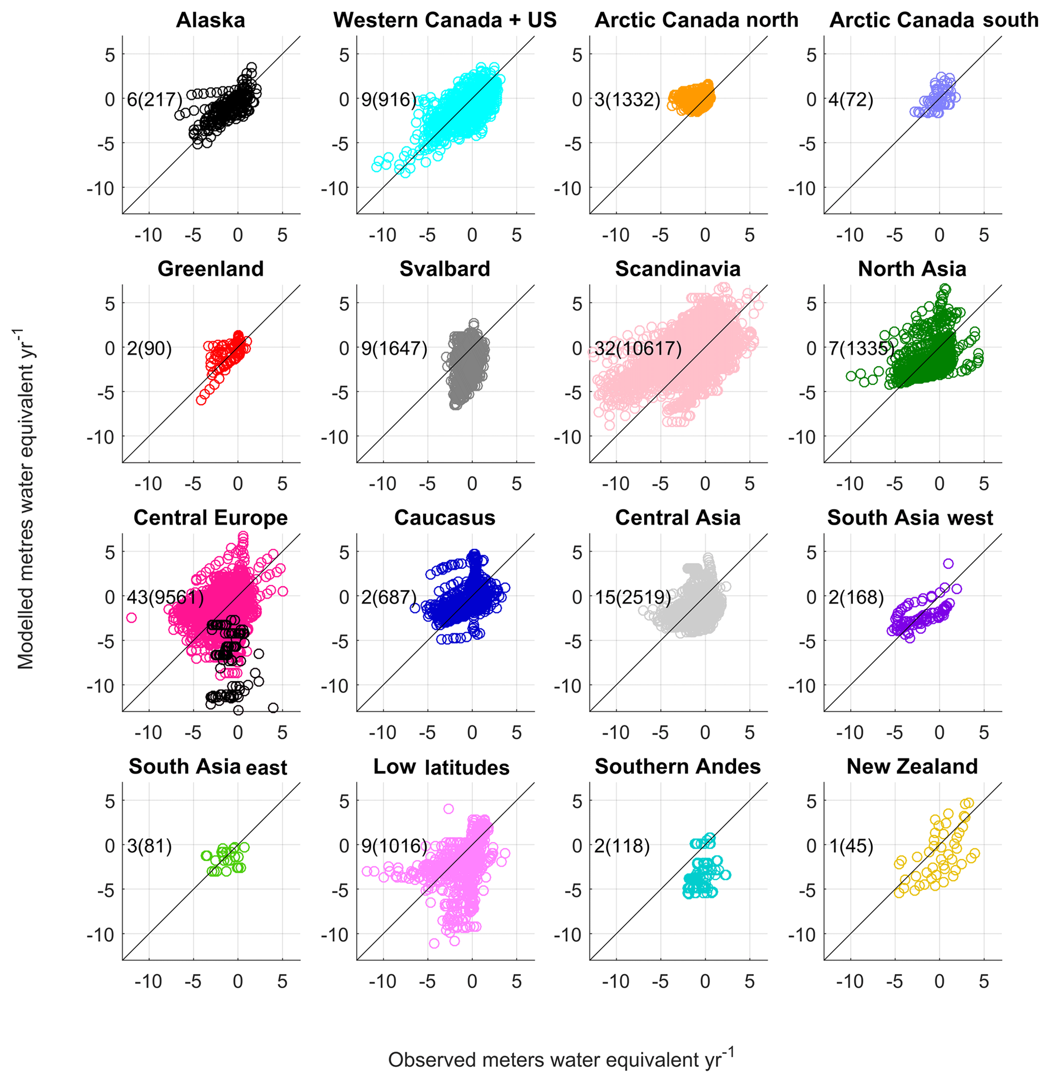
Figure 3Modelled annual elevation-dependent specific mass balance against observations from the WGMS. The modelled mass balance is simulated on a 0.5∘ grid resolution at 250 m elevation bands and the observations are for individual glaciers at elevation levels specific to each glacier. The observed mass balance is interpolated onto the JULES elevation bands. If only a single observation exists, then mass balance for the nearest JULES elevation band is used. The number of glaciers is shown in the top left-hand corner and the number of observation points in brackets. In central Europe mass balance for the Maladeta glacier in the Pyrenees is shown in black circles.
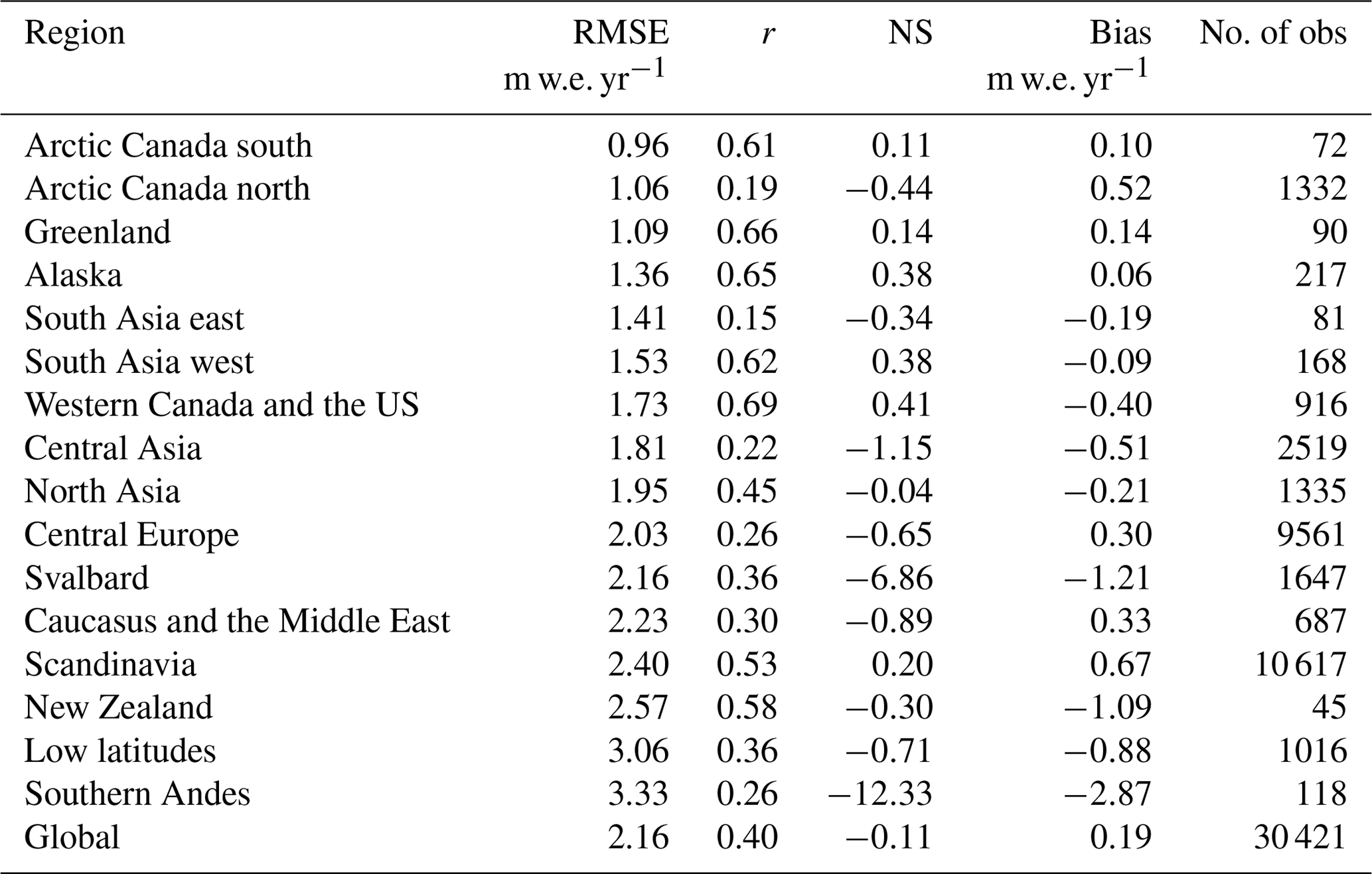
Figure 3 shows the modelled mass balance profiles plotted against the observations using the best parameter set for each region. The best regional parameter sets are listed in Table 2 and the root-mean-square error, correlation coefficient, Nash–Sutcliffe efficiency coefficient, and mean bias are listed in Table 3. Nine out of the 16 regions have a negative bias in the annual mass balance. Notably Svalbard, southern Andes, and New Zealand underestimate mass balance by 1 m w.e. yr−1. The negative bias is also seen in the summer and winter mass balance and discussed in Sect. 3.2. The model performs particularly poorly for the low-latitude region, which has a large RMSE (3.02 m w.e. yr−1). This region contains relatively small tropical glaciers in Colombia, Peru, Ecuador, Bolivia, and Kenya. Marzeion et al. (2012) found a poor correlation with observations in the low-latitude region when they calibrated their glacier model using Climatic Research Unit (CRU) data (Mitchell and Jones, 2005). They attributed that to the fact that sublimation was not included in their model, a process which is important for the mass balance of tropical glaciers. Our mass balance model includes sublimation, so it is possible the WFDEI data over tropical glaciers are too warm. The WFDEI data are based on the ERA-Interim reanalysis in which air temperature has been constrained using CRU data. The CRU data comprise temperature observations which are sparse in regions where tropical glaciers are located. Furthermore, the quality of the WFDEI data will depend on the performance of the underlying ECMWF model. In central Europe some of the poor correlations with observations are caused by the Maladeta glacier in the Pyrenees (Fig. 3), which is a small glacier with an area of 0.52 km2 (WGMS, 2017). When this glacier is excluded from the analysis the correlation coefficient increases from 0.26 to 0.35 and the RMSE decreases from 2.03 to 1.73 m of water equivalent per year.
Table 2Best parameter sets for each RGI6 region. The regions are ranked from the lowest to the highest RMSE. There are no observed profiles for Iceland and the Russian Arctic, so the global mean parameter values are used (bold) for the future simulations.
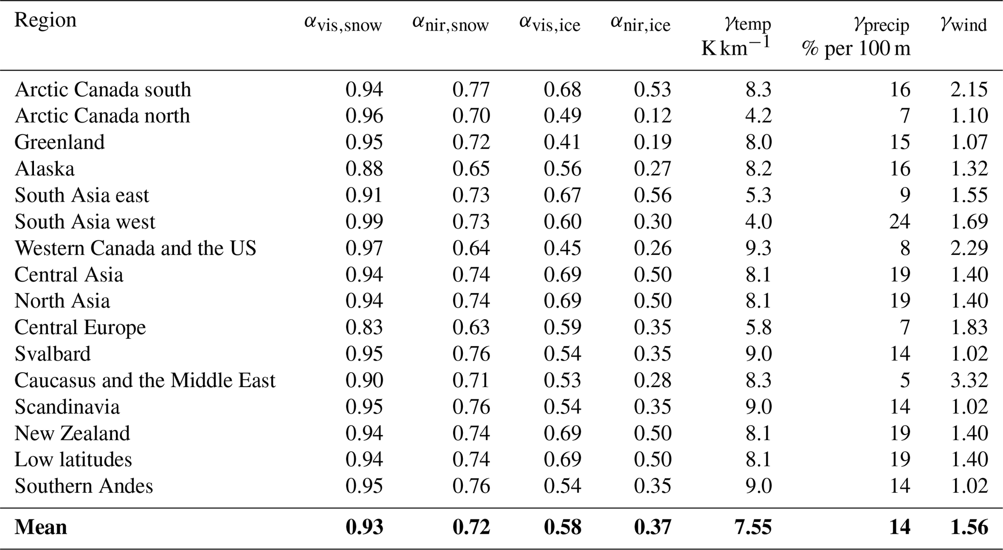
Table 3Root-mean-square error (RMSE), correlation coefficient (r), Nash–Sutcliffe efficiency coefficient (NS), mean bias (Bias), and the number of elevation-band mass balance observations (No. of obs) for RGI6 regions. The regions are ranked from the lowest to the highest RMSE.
3.2 Model validation
The calibrated mass balance is validated against summer and winter elevation-band specific mass balance for each region where data are available (Fig. 4). For all regions, except Scandinavia in the summer, negative Nash–Sutcliffe numbers are calculated for winter and summer elevation-dependent mass balance (Table 4). The negative numbers arise because the bias in the model is larger than the variance of the observations. There are negative biases for nearly all regions, implying that melting is overestimated in the summer and accumulation is underestimated in the winter. This means that future projections of volume loss presented in Sect. 4.2 might be overestimated.

Figure 4Comparison between modelled and observed elevation-band specific mass balance for winter (grey triangles) and summer (black dots). The modelled mass balance is calculated using the tuned regional parameters from the calibration procedure.
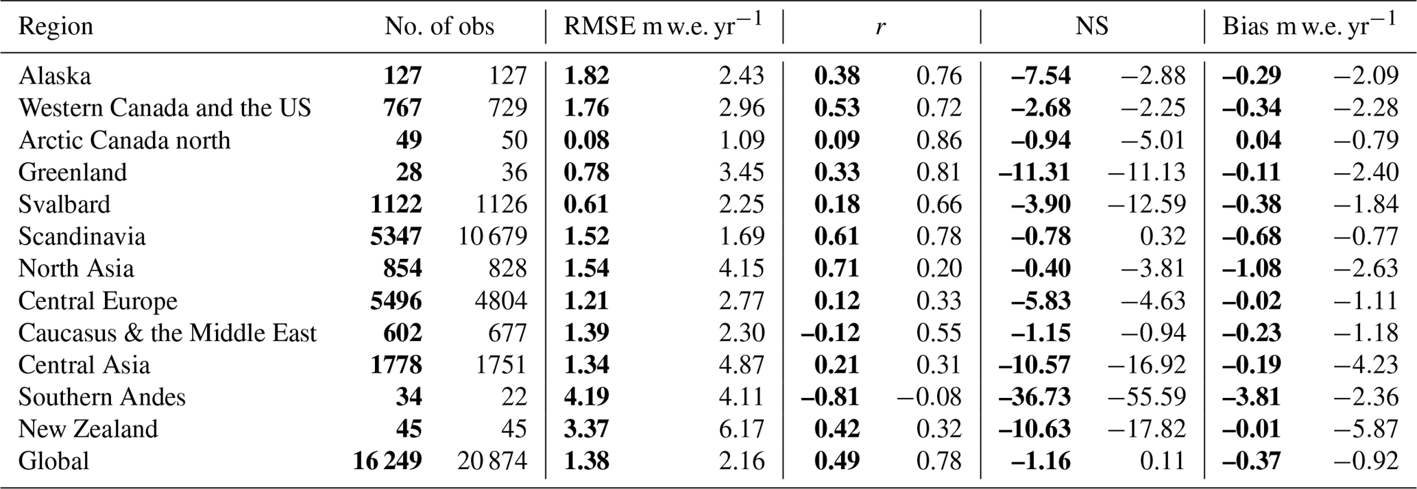
Table 4Winter (bold) and summer number of elevation-band mass balance observations (No. of obs), root-mean-square error (RMSE), correlation coefficient (r), Nash–Sutcliffe efficiency coefficient (NS), and mean bias (Bias).
The reason for the negative bias is because the model underestimates the precipitation and therefore the accumulation part of the mass balance is underestimated. This is because our approach to correcting the coarse-scale gridded precipitation for orographic effects is simple. We use a single precipitation gradient for each RGI6 region and do not apply a bias correction. A bias correction is often recommended because precipitation is underestimated in coarse-resolution datasets. Gauging observations are sparse in high-mountain regions and snowfall observations can be susceptible to undercatch by 20 %–50 % (Rasmussen et al., 2012). Our precipitation rates are generally too low because we do not bias-correct the precipitation.
Other studies use a bias correction that varies regionally (Radić and Hock, 2011; Radić et al., 2014; Bliss et al., 2014). In those studies, the precipitation at the top of the glacier was estimated using a bias correction factor kp. The decrease in precipitation from the top of the glacier to the snout was calculated using a precipitation gradient. To account for the fact that the mass balance of maritime and continental glaciers responds differently to precipitation changes, kp was related to a continentality index. Our motivation for using a single precipitation gradient for each RGI6 region and no bias correction was to test the simplest approach first; however the resulting biases suggest that this approach could be improved.
The impact of underestimating the precipitation is that we simulate negative mass balance in winter at some observational sites (Figs. 5a and 4). To demonstrate this, we compare the mass balance components for two glaciers: the Leviy Aktru in the Russian Altai Mountains, which has negative mass balance in the winter, and Kozelsky glacier in northeastern Russia, which has no negative mass balance in the winter (See Fig. S9). Both glaciers are in the north Asia RGI6 region, so they have the same tuned parameters for mass balance. The simulated winter accumulation rates are much lower at Leviy Aktru glacier than Kozelsky glacier, leading to negative mass balance at the lowest three model levels below 2750 m.
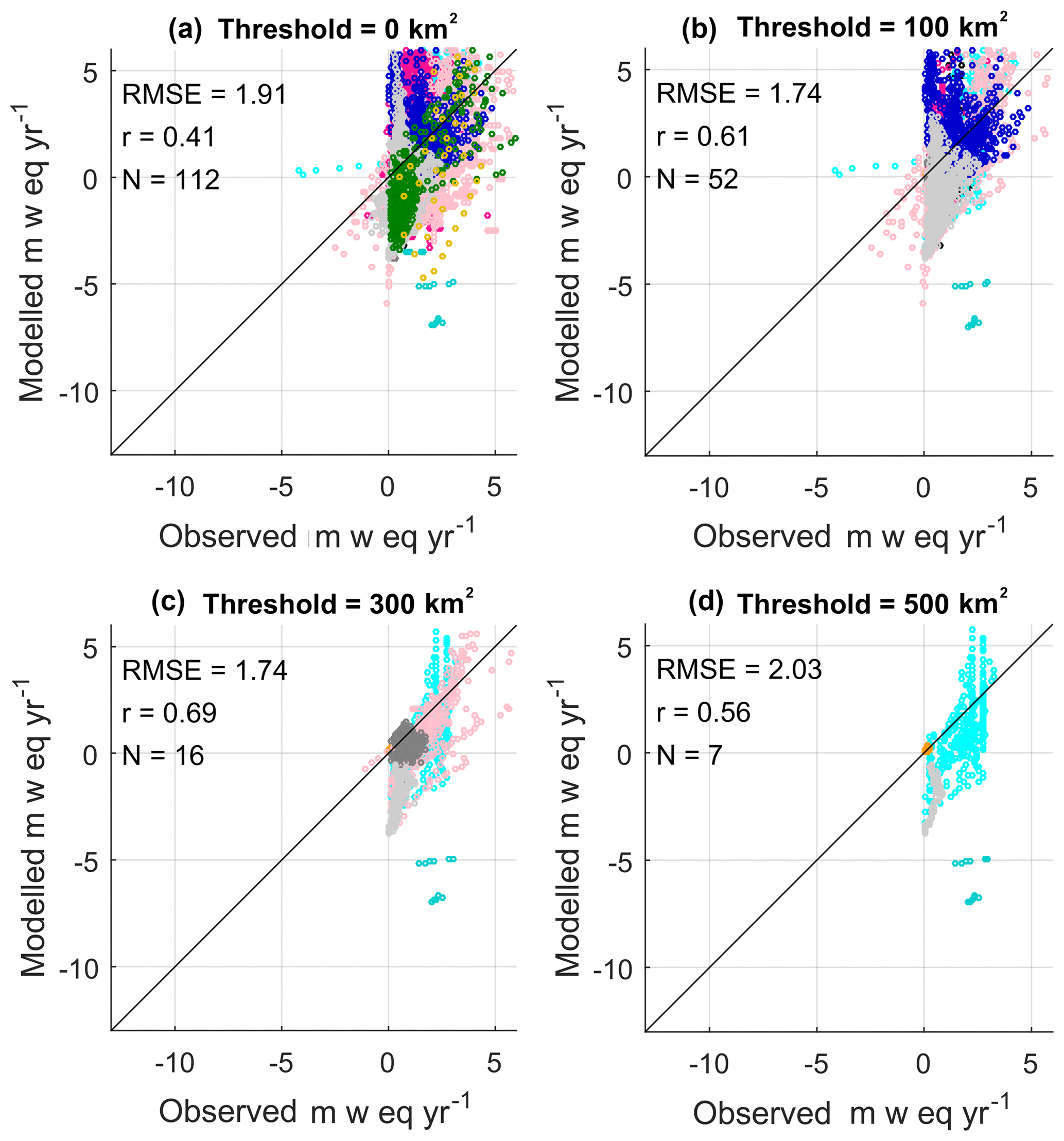
Figure 5Simulated and observed elevation-dependent winter mass balance when grid boxes with a glacier area of less than 100, 300, and 500 km2 are excluded. The colour identifies the RGI6 regions shown in Fig. 2. The RMSE, correlation coefficient, and number of glaciers are listed.
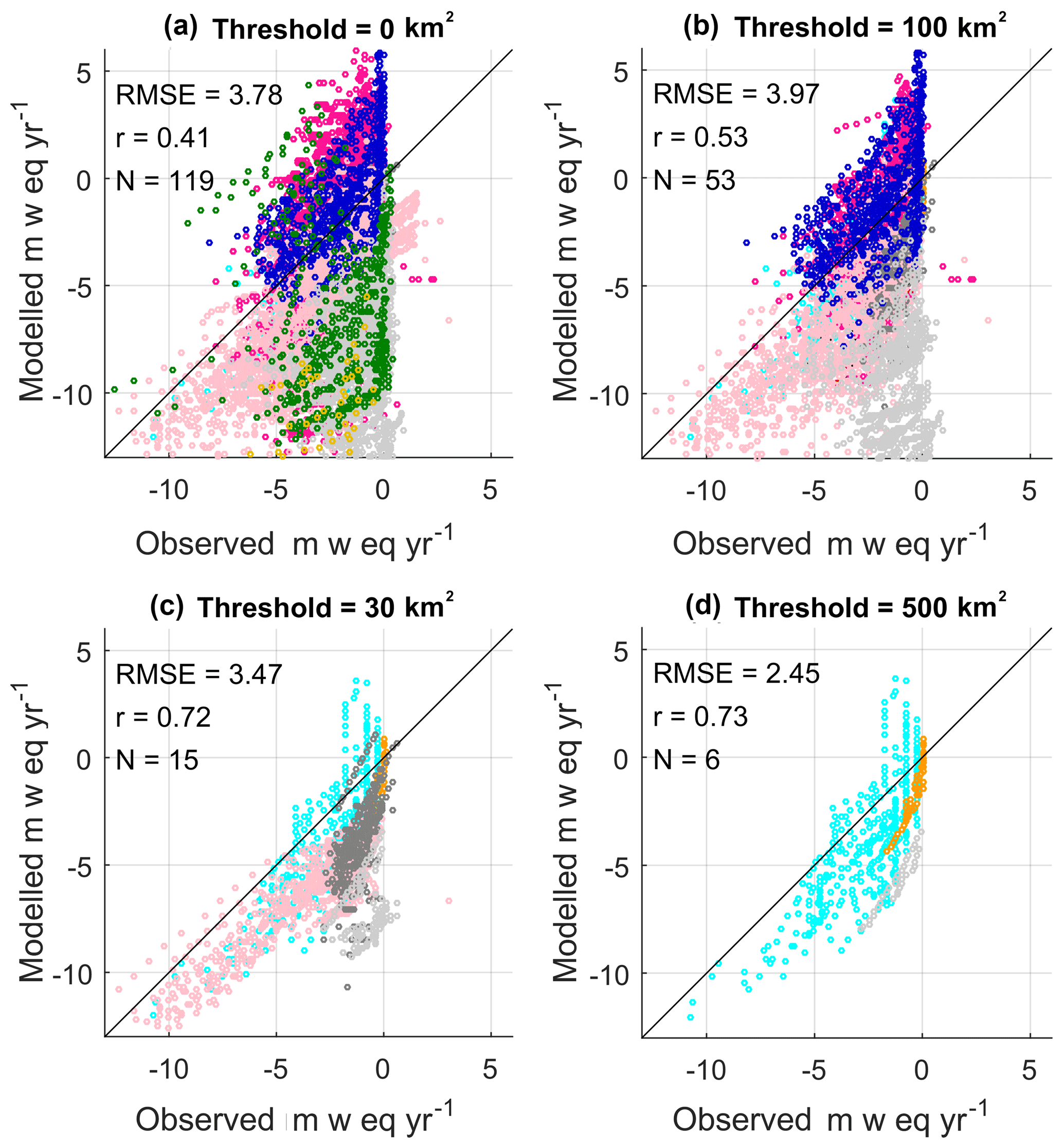
Figure 6Simulated and observed elevation-dependent summer mass balance when grid boxes with a glacier area of less than 100, 300, and 500 km2 are excluded. The colour identifies the RGI6 regions shown in Fig. 2. The RMSE, correlation coefficient, and number of glaciers are listed.
The simplistic treatment of the precipitation lapse rate also leads to instances in which the model simulates positive mass balance in the summer at some locations (Figs. 6a and 4). We show the summer mass balance components for the same two glaciers in Fig. S10. Positive mass balance is simulated at Kozelsky glacier because accumulation exceeds the melting. This suggests that the precipitation gradient (19 % per 100 m for north Asia) is overly steep in the summer at this location.
Another reason we underestimate the accumulation is due to the partitioning of rain and snow based on an air temperature threshold of 0 ∘C. The 0 ∘C threshold is likely too low, resulting in an underestimate of snowfall. When precipitation falls as rain or snow it adds liquid water or ice to the snowpack. The specific heat capacity of the snowpack is a function of the liquid water (Wk) and ice content (Ik) in each layer (k)
where Cice=2100 JK−1 kg−1 and Cwater=4100 JK−1 kg−1. The liquid water content is limited by the available pore space in the snowpack; therefore changes in the snowfall (ice content) control the overall heat capacity. The underestimate in the ice content reduces the heat capacity, which causes more melting than observed.
Other modelling studies have used higher air temperature thresholds: 1.5 ∘C (Huss and Hock, 2015; Giesen and Oerlemans, 2012), 2 ∘C (Hirabayashi et al., 2010), and 3 ∘C (Marzeion et al., 2012). An improved approach would use the wet-bulb temperature to partition rain and snow, which would include the effects of humidity on temperature. Alternatively, a spatially varying threshold based on precipitation observations could be used. Jennings et al. (2018) showed, by analysing precipitation observations, that the temperature threshold varies spatially and is generally higher for continental climates than maritime climates.
Winter mass balance is simulated better than summer mass balance, which is seen by the lower root-mean-square errors for winter in Table 4. Furthermore, the biases are larger in the summer than in the winter (Table 4). It is likely that the simple albedo scheme, which relates albedo to the density of the snowpack surface, performs better in the winter when snow is accumulating than in summer when there is melting. Figures 5b–d and 6b–d show the winter and summer mass balances for all observation sites when area thresholds of 100, 300, and 500 km2 are applied to the validation. There is an improvement in the simulated summer mass balance when the glaciated area increases. This is seen by the improved correlation in Fig. 6d in which the validation is repeated but only grid boxes with a glaciated area greater than 500 km2 are considered. This indicates the model is better at simulating summer melting over regions with a large ice extent than over regions with a small glaciated area.
Table 5List of high-end climate change CMIP5 models that are downscaled using HadGEM3-A. The years when the CMIP5 models pass +1.5, +2, and +4 ∘C global average warming relative to the pre-industrial period are shown.

* No data are available for 2113 because the bias-corrected data end at 2097.
4.1 Downscaled climate change projections
Glacier volume projections are made for all regions, excluding Antarctica, for a range of high-end climate change scenarios. This is defined as climate change that exceeds 2 and 4 ∘C global average warming, relative to the pre-industrial period (Gohar et al., 2017). Six models fitting this criterion were selected from the Coupled Model Intercomparison Project Phase 5 (CMIP5). A new set of high-resolution projections were generated using the HadGEM3-A Global Atmosphere (GA) 6.0 model (Walters et al., 2017). The sea surface temperature and sea ice concentration boundary conditions for HadGEM3-A are supplied by the CMIP5 models. All models use the RCP8.5 “business as usual” scenario and cover a wide range of climate sensitivities, with some models reaching 2 ∘C global average warming relative to the pre-industrial period, quickly (IPSL-CM5A-LR) or slowly (GFDL-ESM2M) (Table 5). The models also cover a range of extreme wet or dry climate conditions. This is important to consider for glaciers in the central and eastern Himalayas, which accumulate mass during the summer months due to monsoon precipitation (Ageta and Higuchi, 1984) and because future monsoon precipitation is highly uncertain in the CMIP5 models (Chen and Zhou, 2015).
The HadGEM3-A data are bias-corrected using a trend-preserving statistical bias method that was developed for the first Inter-Sectoral Impact Model Intercomparison Project (ISIMIP) (Hempel et al., 2013). This technique uses WATCH forcing data (Weedon et al., 2011) to correct offsets in air pressure, temperature, longwave and shortwave downward surface radiation, rainfall, snowfall, and wind speed but not specific humidity. The method adjusts the monthly mean and daily variability in the GCM variables but still preserves the long-term climate signal. The HadGEM3-A was bilinearly interpolated from its native resolution of N216 (∼60 km), onto a 0.5∘ grid, to match the resolution of the WATCH forcing data, which were used for the bias correction. The daily bias-corrected surface fields from the HadGEM3-A are used to run JULES offline to calculate future glacier volume changes. The bias correction was only applied to data up until the year 2097, which means the glacier projections terminate at this year. A flow chart of the experimental setup is shown in Fig. 7. The HadGEM3-A climate data were generated and bias-corrected for the High-End cLimate Impact and eXtremes (HELIX) project.
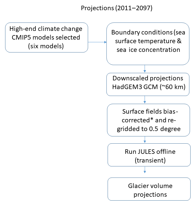
Figure 7Flow chart showing the experimental setup to calculate future glacier volume. * The bias correction method is described by Hempel et al. (2013).
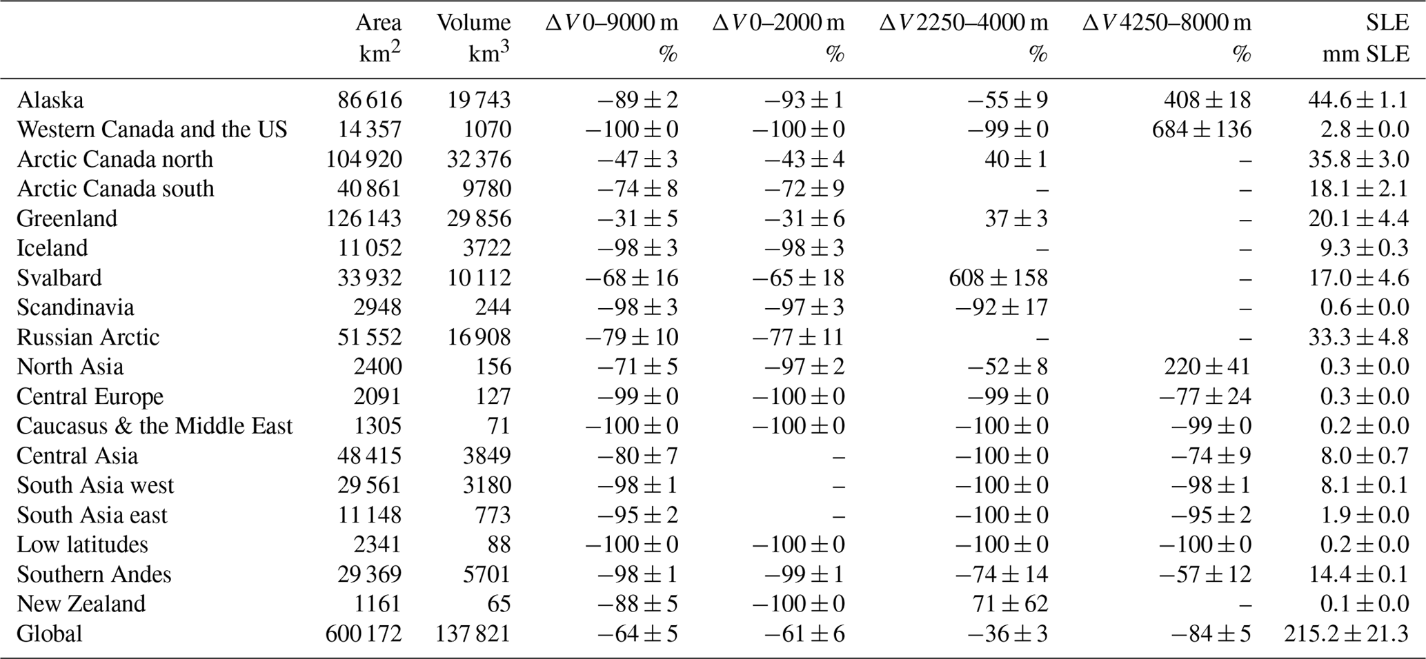
Table 6Percentage ice volume loss, relative to the initial volume (ΔV), and ice loss in millimetres of sea level equivalent (SLE) for the end of the century (2097). Percentage volume losses are shown for low, medium, and high elevation ranges as well as for all elevations. The data show the multi-model mean ± 1 standard deviation. The conversion of volume to SLE assumes an ocean area of 3.618×10⁸ km2. The initial area and volume from the Randolph Glacier Inventory version 6 are listed in columns 1 and 2.
4.2 Regional glacier volume projections 2011–2097
Glaciated areas are divided into 18 regions defined by the RGI6 with no projections made for Antarctic glaciers because the bias correction technique removes the HadGEM3-A data from this region. JULES is run for this century (2011 to 2097) using the best regional parameter sets for mass balance found by the calibration procedure (Table 2). No observations were available to determine the best parameters for Iceland and the Russian Arctic; therefore global mean parameter values are used for these regions. End of the century volume changes (in percent) are found by comparing the volume at the end of the run (2097) to the initial volume calculated from the RGI6. Regional volume changes expressed in percent for low (0–2000 m), medium (2250–4000 m), high (4250–9000 m), and all elevation ranges (0–9000 m) are listed in Table 6. The total volume loss over all elevation ranges is also listed in millimetres of sea level equivalent in Table 6 and plotted in Fig. 10. Maps of the percentage volume change at the end of the century, relative to the initial volume, are contained in the Supplement in Figs. S1–S7.

Figure 8Regional glacier volume projections using the HadGEM3-A ensemble of high-end climate change scenarios.
A substantial reduction in glacier volume is projected for all regions (Fig. 8). Global glacier volume is projected to decrease by 64±5 % by end of the century, for which the value corresponds to the multi-model mean ± 1 standard deviation. The regions which lose more than 75 % of their volume by the end of the century are Alaska ( %), western Canada and the US ( %), Iceland ( %), Scandinavia ( %), the Russian Arctic ( %), central Europe ( %), Caucasus ( %), central Asia ( %), South Asia west ( %), South Asia east ( %), low latitudes (100±0 %), southern Andes ( %), and New Zealand ( %). The HadGEM3-A forcing data show these regions experience a strong warming. In most regions this is combined with a reduction in snowfall relative to the present day, which drives the mass loss (Fig. 9). Regions most resilient to volume losses are Greenland ( %) and Arctic Canada north ( %). In the case of Arctic Canada north, snowfall increases relative to the present day, which helps glaciers to retain their mass. There is a rapid loss of low-latitude glaciers, which has also been found by other global glacier models (Marzeion et al., 2012; Huss and Hock, 2015). Our model overestimates the melting of these glaciers for the calibration period (Fig. 3), so this result should be treated with a degree of caution. Some of the high-latitude regions, particularly Alaska, western Canada and the US, Svalbard, and north Asia, experience very large volume increases at their upper elevation ranges. This would be reduced if the model included glacier dynamics, because ice would be transported from higher elevations to lower elevations. The ensemble mean global sea level equivalent contribution is 215.2±21.3 mm. The largest contributors to sea level rise are Alaska (44.6±1.1 mm), Arctic Canada north and south (34.9±3.0 mm), the Russian Arctic (33.3±4.8 mm), Greenland (20.1±4.4), high-mountain Asia (combined central Asia and South Asia east and west), (18.0±0.8 mm), southern Andes (14.4±0.1 mm), and Svalbard (17.0±4.6 mm). These are the regions which have been observed by the Gravity Recovery and Climate Experiment (GRACE) satellite to have lost the most mass in the recent years (Gardner et al., 2013).

Figure 9Regional temperature and snowfall changes relative to the present day (2011–2015) from the HadGEM3-A ensemble over glaciated grid points. The ensemble mean is shown in the solid line and the range of model projections are shown in the shaded regions.
To investigate which parts of the energy balance are driving the future melt rates, we show the energy balance components averaged over all regions and all elevation levels in Fig. 11. Future melting is caused by a positive net radiation of approximately 30 W m−2 that is sustained throughout the century. This is comprised of 18 W m−2 net shortwave radiation, 3 W m−2 net longwave radiation, 5 W m−2 latent heat flux, and 4 W m−2 sensible heat flux. The largest component of the radiation for melting comes from the net shortwave radiation. The upward shortwave radiation comprises direct and diffuse components in the VIS and NIR wavelengths. The VIS albedo decreases because melting causes the ice surface to darken. In contrast, the NIR albedo increases because the ice is heating up, emitting radiation in the infrared part of the spectrum.
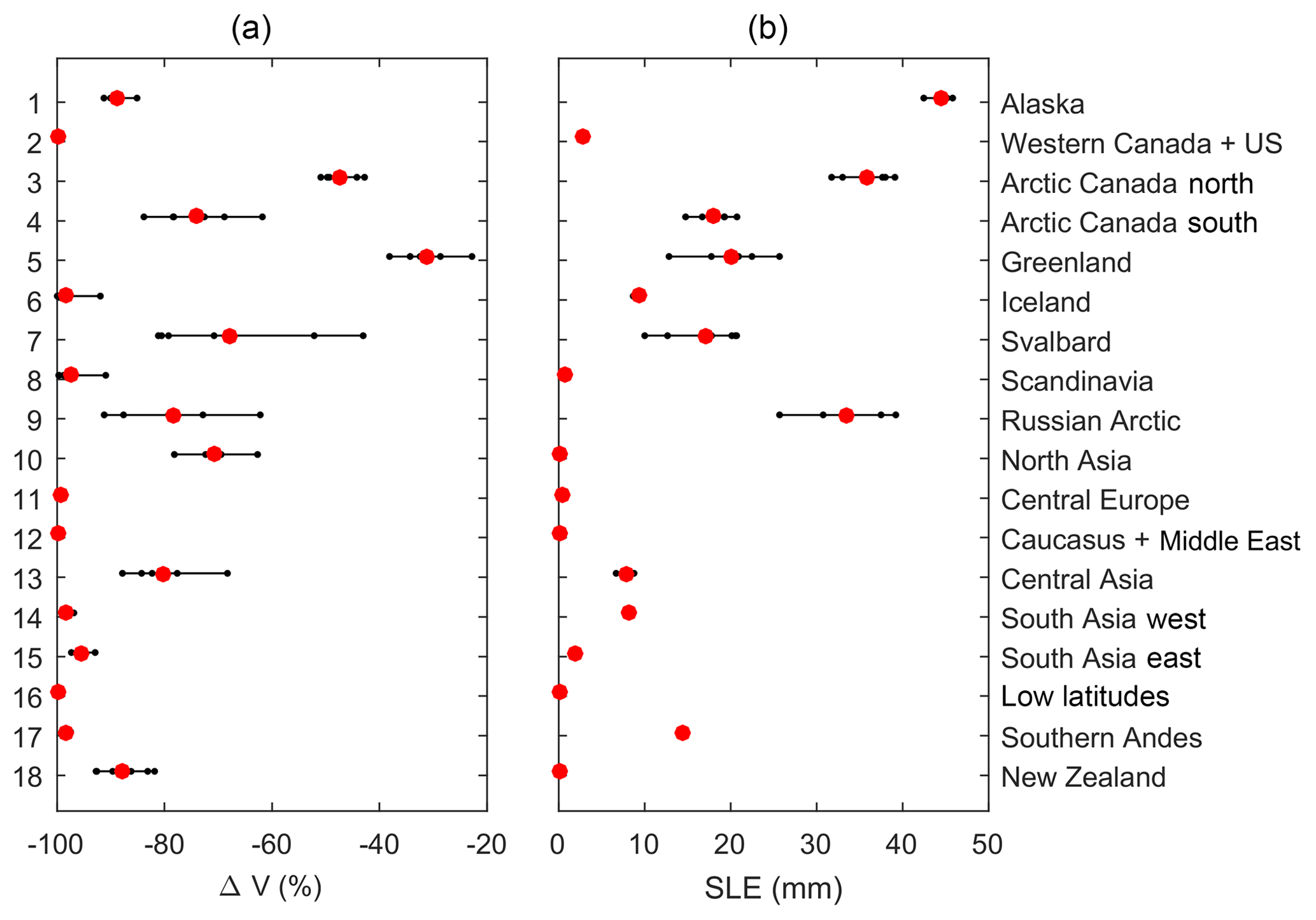
Figure 10(a) Regional percentage volume losses at the end of the century (2097), relative to the initial volume and (b) volume losses expressed in sea level equivalent contributions. The large red dots represent the multi-model mean and the small black dots are the individual HadGEM3-A model runs.

Figure 11Ensemble mean energy balance components averaged over all glaciated regions and all elevation bands when the model is forced with HadGEM3-A data.
The downward and upward longwave radiation are increasing in the future; however, the net longwave radiation contribution to the melting is small. The downward longwave radiation increases because of the T4 relationship with air temperature, whereas the upward longwave radiation increases because the glacier surface is warming. The latent heat flux from refreezing of meltwater and the sensible heat from surface warming are also small components of the net radiation balance.
4.3 Mass balance components
In this section we examine how the surface mass balance components vary with height and how this will change in the future. Figure 12 shows the accumulation, refreezing, and melting contributions to mass balance averaged over low, medium, and high elevation ranges for the period 1980–2000. Sublimation is excluded because its contribution to mass balance is relatively small. As expected, there is more melting in the lower elevation ranges and more accumulation at the higher elevation ranges. The refreezing component, which includes refreezing of meltwater and elevated adjusted rainfall, shows no clear variation with height. This is because the refreezing component can both increase and decrease with height. Refreezing can increase towards lever elevations because there is more rain and melted water. It can also decrease if the snowpack is depleted or if there is not enough pore space to hold water because previous refreezing episodes have converted the firn into solid ice. The largest accumulation rates occur in Alaska (5.3 m w.e. yr−1) and western Canada and the US (7.3 m w.e. yr−1) between 4250 and 9000 m and the largest melt rates are found in the Caucasus and Middle East (−7.4 m w.e. yr−1) and the low latitudes (−7.6 m w.e. yr−1).
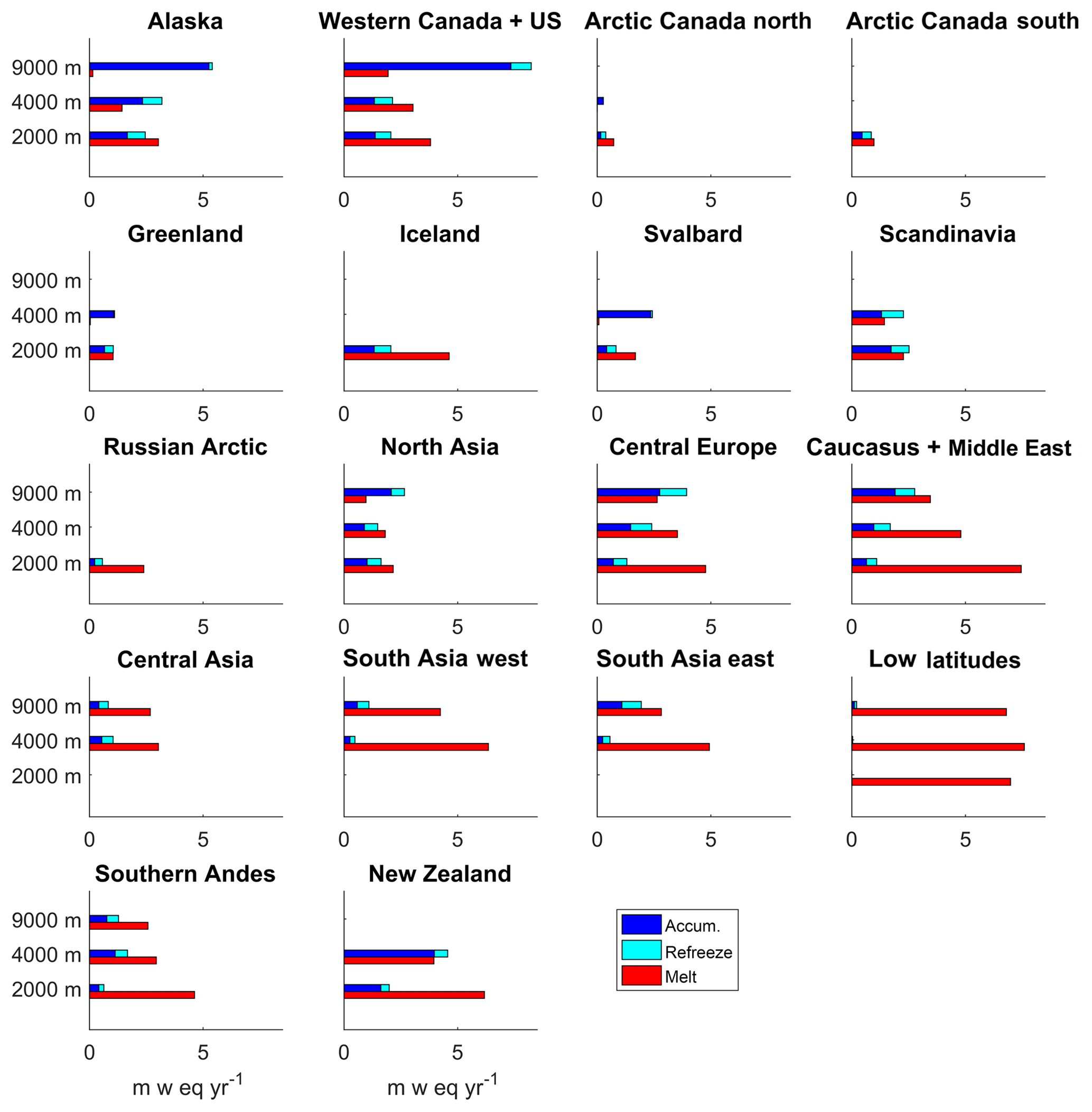
Figure 12Modelled annual surface mass balance components: accumulation, refreezing, and melting for the period 1980–2000 for RGI6 regions. To make the figure easier to read, melting is given as a positive sign and sublimation is excluded because its contribution is very small. Mass balance components are averaged over low (0–2000 m), medium (2250–4000 m), and high (4250–9000 m) elevation ranges.

Figure 13Global mass balance components for three elevation ranges. The historical period is calculated using the WFDEI data and the future period is the multi-model means of all GCMs. The bars show the averages over the time periods for accumulation, refreezing, melt, and mass balance rates.
Figure 13 shows how the global annual mass balance components vary with time for low, medium, and high elevation ranges.
There is a reduction in accumulation and refreezing at all elevation ranges towards the end of the century. Melt rates decrease at medium and high elevation ranges because glacier mass is lost at these altitudes; therefore less ice is available to melt (see Fig. S8 for the future cumulated mass balances as a function of height). Melt rates are constant at the low elevation ranges because there remain substantial quantities of ice available to melt at the end of the century in Greenland, Arctic Canada north and south, Svalbard, and the Russian Arctic. At high elevations mass balance is reduced from −2.2 m w.e. yr−1 (−177 Gt yr−1) during the historical period (1980–2000) to −0.35 m w.e. yr−1 (−28 Gt yr−1) by the end of the century (2080–2097). Similarly, for the medium elevation ranges mass balance decreases from −0.56 m w.e. yr−1 (−26 Gt yr−1) to −0.24 m w.e. yr−1 (−11 Gt yr−1).
4.4 Parametric uncertainty analysis
The standard deviation in the volume losses presented above are relatively small. This is because only a single GCM was used to downscale the CMIP5 data (HadGEM3-A). The uncertainty in the ensemble mean reflects the impact of the different sea surface temperature and sea ice concentration boundary conditions, provided by the CMIP5 models, on the HadGEM3-A climate. Other sources of uncertainty in the projections can arise from the calibration procedure, observational error, initial glacier volume and area, and structural uncertainty in the model physics. It is beyond the scope of this paper to investigate all the possible sources of uncertainty on the glacier volume losses. Instead we discuss the impact of parametric uncertainty in the calibration procedure in the following section.
In the calibration procedure the mass balance was tuned to obtain an optimal set of parameters for each RGI6 region; however, there may be other plausible parameter sets that perform equally well (i.e. for which the RMSE between the observations and the model is small). The principle of “equifinality”, in which the end state can be reached by many potential means, is important to explore because some parameters may compensate for each other. For example, the same mass balance could be reached by increasing the wind scale factor, which enhances melting, or decreasing the precipitation gradient, which would reduce accumulation. To identify the experiments that perform equally well, we identify where there is a step change in the gradient of the RMSE for each RGI6 region. A similar approach was used by Stone et al. (2010) to explore the uncertainty in the thickness, volume, and areal extent of the present-day Greenland ice sheet from an ensemble of Latin hypercube experiments. The step change in the RMSE is identified using the change-point detection algorithm called findchangepts (Rebecca et al., 2012; Lavielle, 2005) from the MATLAB signal processing toolbox. The algorithm is run to find where the mean of the top 10 experiments (excluding the optimal experiment) changes the most significantly. For each RGI6 region the step changes in the RMSE are shown in Fig. 14.
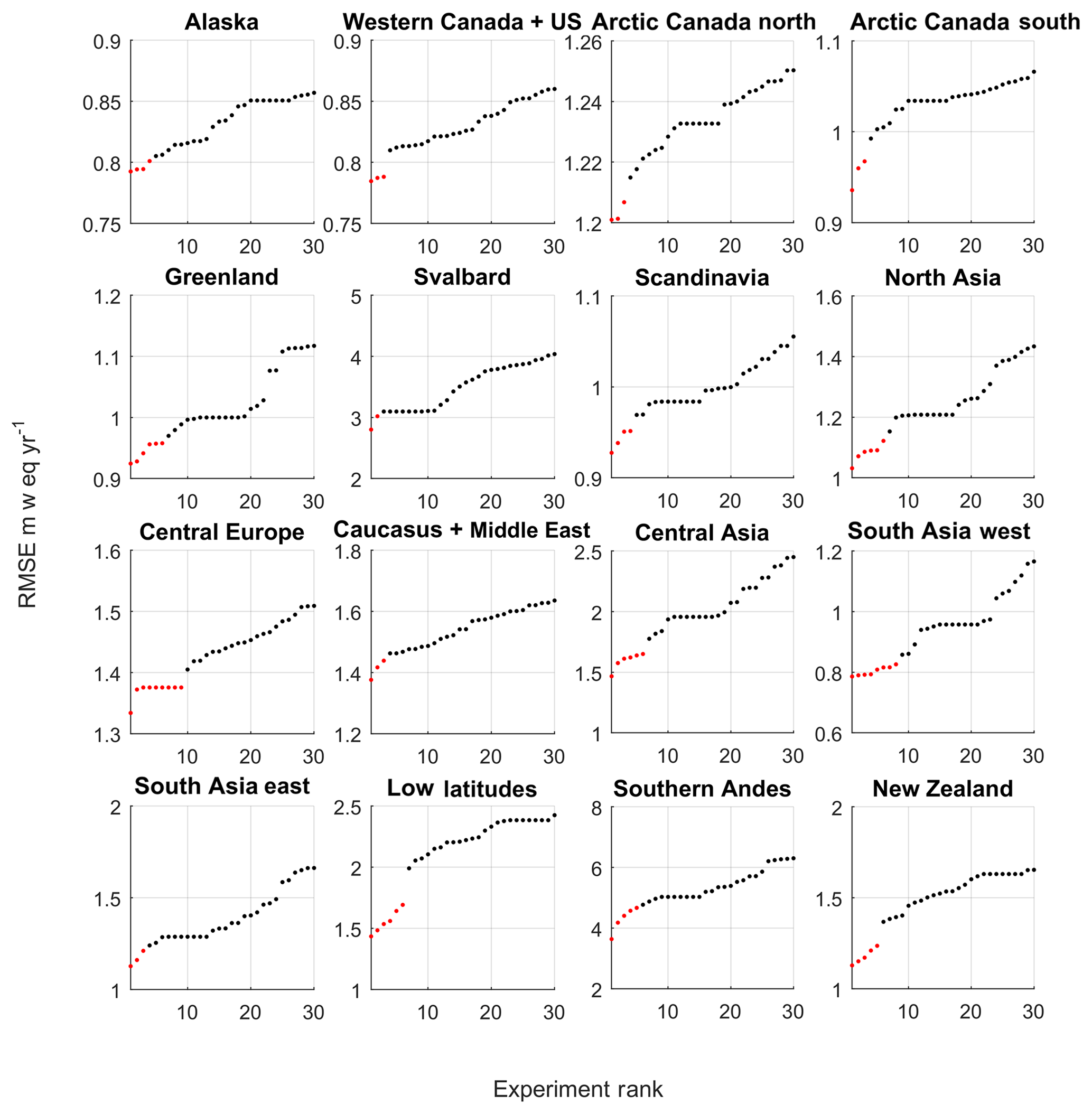
Figure 14Calibration experiments ranked according the root-mean-square error between simulated and observed mass balance profiles for RGI6 regions. There are 198 experiments but only the top 30 have been plotted to make the figure easier to read. The red dots indicate experiments that perform equally well.
JULES is rerun for each of the downscaled CMIP5 experiments and for each parameter set that is defined as performing equally well (see Table S1 in the Supplement for a list of the parameter sets that perform equally well). The volume losses expressed in millimetres of sea level equivalent are shown in Fig. 15. The effects of the parametric uncertainty on the volume losses vary regionally, with the largest impact found for central Europe and Greenland. Regional volume losses including parametric uncertainty in the calibration are summarised in Table 7. Including calibration uncertainty in this way gives an upper bound of 247.3 mm of sea level equivalent volume loss by the end of the century.
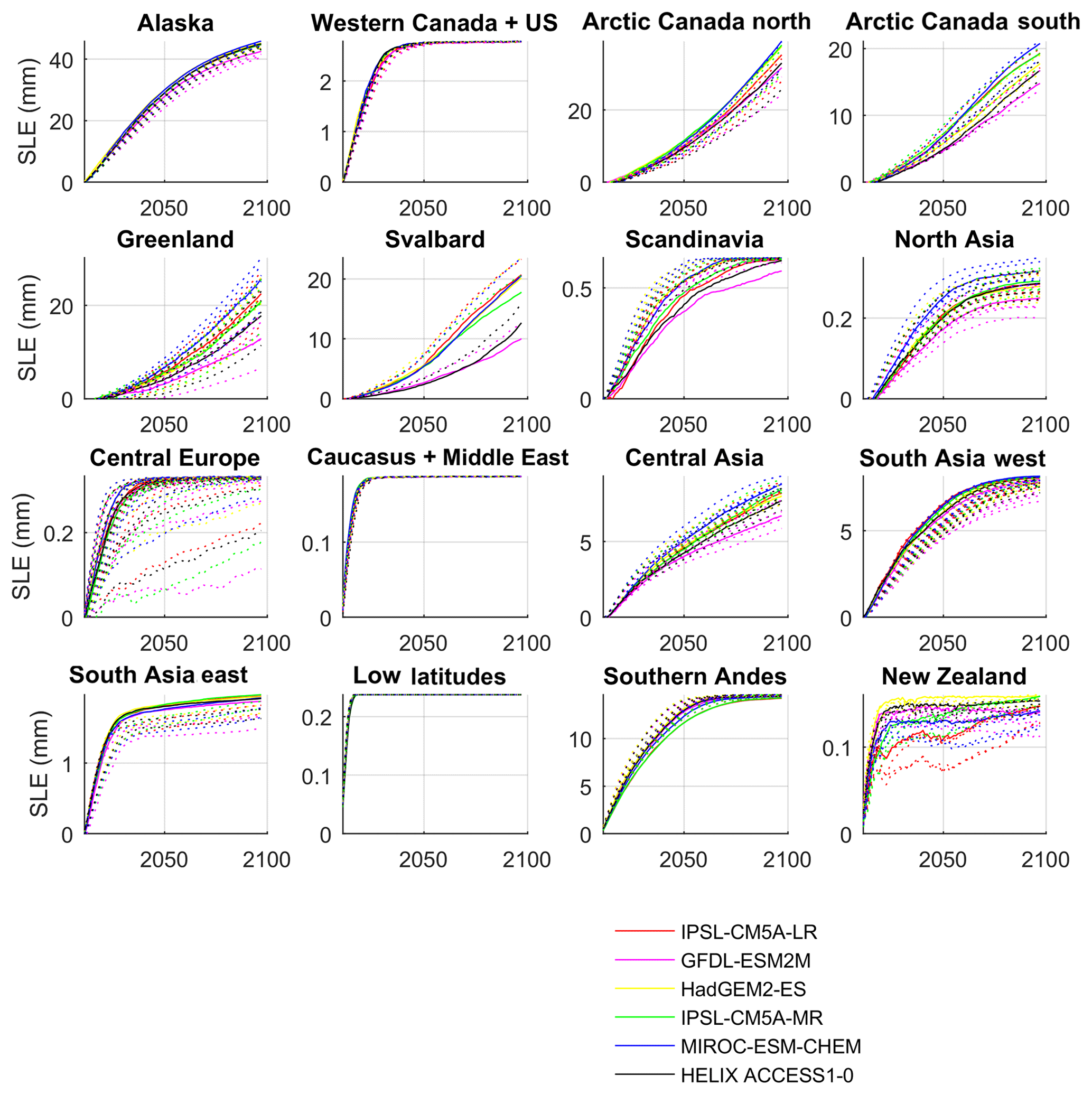
Figure 15Regional volume losses expressed in sea level equivalent including parametric uncertainty in mass balance parameters. The solid lines show the volume loss for each downscaled CMIP5 GCM using the optimum parameter sets. The dashed lines are for runs which use other equally “good” parameter sets based on the RMSE.
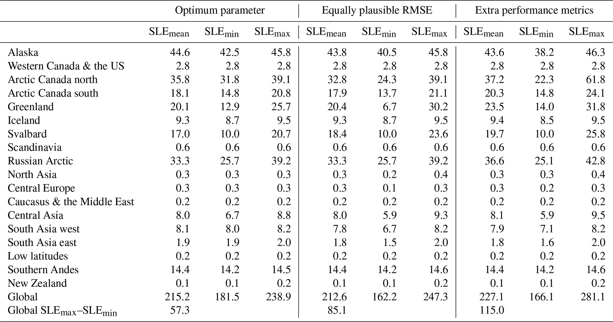
Table 7Regional ensemble mean, minimum, and maximum volume losses for 2097 in sea level equivalent (mm) when the present-day mass balance is calibrated in different ways. Columns 1–3: mass balance is calibrated by minimising the RMSE. Columns 4–6: mass balance is calibrated using an ensemble of equally plausible RMSE values. Columns 7–9: mass balance is calibrated by minimising the RMSE, minimising the bias, and maximising the correlation coefficient.
Another way to explore the uncertainty in the volume projections caused by the calibration procedure is to use different performance metrics to identify the best parameter sets. In addition to using RMSE, we calculate the best parameter sets by (1) minimising the absolute value of the bias and (2) maximising the correlation coefficient. The best regional parameter sets are different depending on the choice of performance metric used (see Tables S2 and S3 in the Supplement). For 12 regions, minimising the bias results in higher precipitation lapse rates than when RMSE values are used to select parameters. This suggests the bias in many regions is caused by underestimating the precipitation lapse rates. As discussed above, this could be due to the fact the grid box mean WFDEI precipitation was not bias-corrected. Glacier volume projections are generated by repeating the simulations using these two additional performance metrics to identify the best parameter sets. The uncertainty in the global volume loss when the extra performance metrics are used is approximately double the uncertainty arising from the different climate forcings (Fig. 16, Table 7). When extra performance metrics are used, the upper bound volume loss increases to 281.1 mm of sea level equivalent by the end of the century.
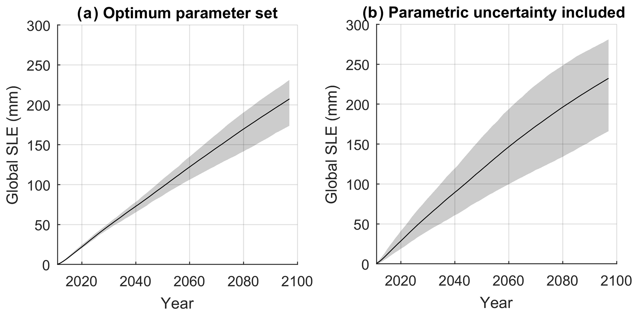
Figure 16Multi-model mean (black line) and ensemble spread (shaded) global volume loss in sea level equivalent. Panel (a) shows the volume loss when optimum parameter sets are selected by minimising the RMSE and (b) is volume loss when optimum parameter sets are selected using additional performance metrics (minimising RMSE, minimising the bias, and maximising the correlation coefficient).
4.5 Comparison with other studies
We compare our end-of-the-century volume changes (excluding parametric uncertainty) to two other published studies which used the CMIP5 ensemble under the RCP8.5 climate change scenario (Huss and Hock, 2015; Radić et al., 2014). Other studies exist, but these include the volume losses from Antarctic glaciers, which makes a direct comparison difficult (Marzeion et al., 2012; Slangen et al., 2014; Giesen and Oerlemans, 2013; Hirabayashi et al., 2013). Huss and Hock (2015) listed regional percentage volume change and sea level equivalent values in their study while Radić et al. (2014) listed sea level equivalent values only (see the comparison of Tables S4 and S5 in the Supplement).
Our end-of-the-century percentage volume losses compare reasonably well to Huss and Hock (2015) for central Europe, Caucasus, South Asia east, Scandinavia, the Russian Arctic, western Canada and the US, Arctic Canada north, north Asia, central Asia, low latitudes, and New Zealand but are significantly higher in the southern Andes, Alaska, Iceland, and Arctic Canada south. The uncertainty in our percentage volume losses is smaller than that of Huss and Hock (2015) because we only use a single GCM to downscale the CMIP5 experiments while Huss and Hock (2015) use 14 CMIP5 GCMs.
We estimate the end-of-century global sea level contribution, excluding Antarctic glaciers, to be 215±20 mm, which is higher than 188 mm (Radić et al., 2014) and 136±23 mm (Huss and Hock, 2015) caused mainly by greater contributions from Alaska, southern Andes, and the Russian Arctic. These three regions are discussed in turn.
For the southern Andes our estimates are approximately double (14.4 mm) those of the other studies (5.8 mm, Huss and Hock, 2015; 8.5 mm, Radić et al., 2014). This region has the largest negative bias in the calibrated present-day mass balance (−2.87 m w.e. yr−1; see Table 3). To explore the effects of correcting the calibration bias on the ice volume projections, we subtract the bias values listed in Table 3 from the future annual mass balance rates. Each grid box is assumed to have the same regional mass balance bias. The bias-corrected volume losses are listed in Table S5 in the Supplement. For the southern Andes, the volume losses are much closer to the other studies (7.6 mm) when the bias is corrected. The impact is less for the other regions where the biases are smaller. For the Russian Arctic our volume losses are higher than the other studies but that should be interpreted with caution because there were no observations available in this region to obtain a tuned parameter set (global mean parameters were used instead). In Alaska the bias in annual mass balance is small (0.06 m w.e. yr−1), so correcting the bias has little effect on the volume loss projection for this region. Applying the bias correction increases the global volume loss from 215±20 to 223±20 mm; therefore the difference between our model and the other studies cannot be explained by the bias in the calibration.
It is likely that our sea level equivalent contributions are higher than the other studies because the climate forcing data are different. The HadGEM3-A model uses boundary conditions from a subset of RCP8.5 CMIP5 models with the highest warming levels. Furthermore, the HadGEM3-A data have a higher resolution (approximately 60 km) than the CMIP5 data, which were used by the other two studies. This means our model should, in theory, be more accurate at reproducing regional patterns in precipitation and temperature over complex terrain, which is important for calculating mass balance.
The robustness of the glacier projections depends on how well the model can reproduce present-day glacier mass balance. Our calibrated seasonal mass balance contains a negative bias (accumulation is underestimated, and melting is overestimated), which suggests the projections of volume loss might be overestimated. One of the main shortcomings of the calibration and validation of mass balance is that only a single type of observations is used. These data were used because we wanted to ensure the model could reproduce variations in accumulation and ablation with height when the elevated tiling scheme was introduced. Point mass balance observations are affected by local factors such as aspect, avalanching, and debris cover and there is a possibility that these local factors affect parameter sets chosen for the entire RGI region. This could be improved by using observations from satellite gravimetry and altimetry, such as that described by Gardner et al. (2013), to obtain a quantitative estimate of the model performance at the regional scales.
One of the notable differences between our study and other global glacier models is that our tuned precipitation lapse rates are very high, for example, 24 % per 100 m for South Asia west and 19 % per 100 m for central Asia. Other models have used lower precipitation lapse rates (1–2.5 % per 100 m, Huss and Hock, 2015; 3 % per 100 m, Marzeion et al., 2012), but they also bias-correct precipitation by multiplying by a scale factor. This scaling factor can be considerably high. Giesen and Oerlemans (2012) found that precipitation needed to be multiplied by a factor of 2.5 to obtain good agreement with mass balance observations. Radić and Hock (2011) derived, through calibration of present-day mass balance, a precipitation scale factor of as high as 5.6 for Tuyuksu and Golubina glaciers in the Tien Shan. Our lapse rates are high because we do not bias-correct the precipitation using a multiplication factor for the present day. For the future GCM data the grid box mean precipitation was bias-corrected using the ISIMIP technique. The negative bias that we obtain when validating the present-day mass balance suggests that snowfall is underestimated in our model. A future study using this model could test whether bias-correcting the precipitation before applying the lapse rate correction improves the simulated mass balance.
This is the first attempt to implement a glacier scheme into JULES and so the model has many limitations. One of the key shortcomings is that glacier dynamics is not included (glacier area does not vary). The transport of ice from higher elevations to lower elevations is not included. This process could be included in future work by adding a volume–area scaling scheme (Bahr et al., 1997) or a thickness parameterisation based on glacier slope (Marshall and Clarke, 2000). Volume–area scaling has been used to model glacier dynamics in coarse-resolution (0.5∘) models in which all glaciers in a grid box are represented by a single ice body (Kotlarski et al., 2010; Hirabayashi et al., 2010). The current configuration of elevated glaciated and unglaciated tiles in JULES makes it well suited to a volume–area scaling model. This would be implemented by growing (shrinking) the elevated glaciated tiles if mass balance is positive (negative) at each elevation band. In the case in which the elevated ice tile grows the unglaciated tile would shrink at that elevation band or vice versa.
The volume–area scaling law has been used successfully to model the dynamics of individual glaciers (Radić et al., 2014; Giesen and Oerlemans, 2013; Marzeion et al., 2012; Slangen et al., 2014) but has some limitations when applied to coarse models in which glaciers are consolidated into a single grid box. The volume–area scaling law relates volume to area using a constant scaling exponent, which is typically derived from a small sample of glacier observations (Bahr et al., 1997). One of the drawbacks is that the law is non-linear, meaning the exponent derived from individual glaciers would overestimate the volume of a large ice grid box such as in our model (Hirabayashi et al., 2013). Furthermore, the exponent may not accurately represent the volume–area relationship in other geographical regions. To overcome these issues a spatially variable scaling exponent could be created using the newly available 0.5∘ data on volume and area contained in the RGI6.
Another limitation of the model, which may be problematic for same applications, is that the grid box mean precipitation is not conserved when precipitation is adjusted for elevation. This correction was necessary to obtain enough accumulation in the mass balance at high elevations. One way to conserve water mass would be to reduce the precipitation onto the non-glaciated area of the grid cell. This would represent horizontal mass movement within the grid box from windblown snow and avalanching.
A further limitation of the model is the simple treatment of katabatic winds, which is modelled by scaling the synoptic wind speed. This could be improved by parameterising katabatic winds based on the grid box slope and the temperature difference between the glacier surface and the air temperature using the Prandtl model (Oerlemans and Grisogono, 2002). Another drawback of the model is the coarse resolution of the grid boxes, which makes it unfeasible to include some process that affects local mass balance such as hillside shading, avalanching, blowing snow, and calving. The model could, however, be run on a finer resolution using higher-resolution climate forcing data.
While this modelling projects considerable reduction in glacier mass for all mountain ranges by the end of this century, it is clear that many of the world's mountain glaciers will evolve in ways that are currently difficult to model. For instance, paraglacial processes during deglaciation lead to enhanced rock falls and debris flows from deglaciating mountain slopes and these deliver rock debris to glacier surfaces. This produces debris-covered glaciers and these are common in many mountain regions, including in Alaska, the arid Andes, central Asia, and in the Hindu Kush–Himalayas. Thick debris cover (decimetres to metres) limits ice ablation (e.g. Lambrecht et al., 2011; Pellicciotti et al., 2014; Lardeux et al., 2016; Rangecroft et al., 2016) and reverses the mass balance gradient, with comparatively higher ablation rates up-glacier than at the debris-covered terminus. This significantly influences glacier dynamics (Benn et al., 2005), and with inefficient sediment evacuation eventually leads to the transition from debris-covered glaciers to rock glaciers (e.g. Monnier and Kinnard, 2017). In the context of continued climate warming, the transition from ice glaciers to rock glaciers may enhance the resilience of the mountain cryosphere (Bosson and Lambiel, 2016). As a result, better assessment of the response of the mountain cryosphere to climate warming will depend on a clearer understanding of glacier–rock glacier relationships.
There are three key strengths to the JULES glacier model. Firstly, we include variations in orography within a climate grid box, which is important to calculate elevation-dependent glacier mass balance. Kotlarski et al. (2010) developed a glacier scheme for the REMO regional climate model by lumping glaciers into 0–5∘ grid boxes in an approach similar to ours, but they did not have a representation of subgrid orography. Instead glacier grid boxes received double the grid box mean snowfall, glacier ice had a fixed albedo, and a constant lapse rate was applied to adjust temperatures. They concluded that to reproduce mass balance trends over the Alps, the scheme needed to include subgrid variability in atmospheric parameters within a grid box.
Secondly, the model uses a full energy balance scheme to calculate glacier melting. This is a more physically based approach than the widely used temperature index models, which relate melting to temperature using a degree day factor (DDF). The DDF lumps all the energy balance components into a single number, meaning that the effects of changing wind speed, cloudiness, and radiation on melt rates cannot be considered. Changes in solar radiation can be an important driver of melting. Huss et al. (2009) studied long-term mass balance trends for a site in the Alps and showed that melting was stronger during the 1940s than in recent years despite more warming. This was because summer solar radiation was higher during the 1940s. Moreover, temperature index models have been found to be less accurate with increasing temporal resolution (for example on daily time steps) (Hock, 2005). In this paper, we present a brief analysis of the future global energy balance fluxes, but how the fluxes vary for individual regions and elevation levels could be investigated further. Finally, the glacier scheme is coupled to a land surface model, which presents opportunities for further studies. For instance, the model could be used to investigate the impact of climate change on river discharge in glaciated catchments in Asia, South America, or the Arctic.
The first aim of this study was to add a glacier component to JULES to develop a fully integrated model to simulate the interactions among glacier mass balance, river runoff, water abstraction by irrigation, and crop production. To do this we added two new surface types to JULES: elevated glaciated and unglaciated tiles. This allows us to calculate elevation-dependent mass balance, which can be used to study the response of glaciers to climate change. Glacier volume was modelled by growing or shrinking the snowpack, using the elevation-dependent mass balance, but glacier dynamics was not included. Present-day mass balance was calibrated by tuning albedo, wind speed, temperature, and precipitation lapse rates to obtain a set of regionally tuned parameters which are then used to model future mass balance. Winter and summer mass balances are reproduced reasonably well for regions where the glaciated area is large; however, the model performs poorly for small glaciers, particularly in the summer. The fully integrated model is potentially a useful tool for studying the impacts of climate change on water resources in glaciated catchments.
The second aim of this study was to make glacier volume projections for the future under a range of high-end climate change scenarios. The ensemble mean volume loss ± 1 standard deviation is % for all glaciers excluding those on the periphery of the Antarctic ice sheet. The small uncertainties in the multi-model mean are caused by the sensitivity of HadGEM3-A to the boundary conditions supplied by the CMIP5 models. Our end-of-the-century global volume loss is 215±20 mm, which is higher than values reported by other studies. This is because we used a subset of CMIP5 models with the highest warming levels to drive the model and glacier dynamics not included, which results in more mass loss than other studies that include dynamics. Including parametric uncertainty in the calibration procedure results in an upper bound global volume loss of 281.1 mm of sea level equivalent by the end of the century. The projected ice losses will have an impact on sea level rise and on water availability in glacier-fed river systems.
The glacier scheme is included in JULES v4.7. The source code can be downloaded by accessing the Met Office Science Repository Service (MOSRS) (requires registration): https://code.metoffice.gov.uk/ (last access: 23 June 2017). The code used for this study is in https://code.metoffice.gov.uk/svn/jules/main/branches/dev/sarahshannon/vn4.7_va_scaling (last access: 23 June 2017).
The supplement related to this article is available online at: https://doi.org/10.5194/tc-13-325-2019-supplement.
SS wrote the paper and all the co-authors gave input for the writing. SS, RS, and AW contributed to the JULES source code. MH created the 0.5∘ glacier area and thickness data from the RGI6 dataset. JC generated the high-resolution HadGEM3-A data and AK preformed the bias correction.
The authors declare that they have no conflict of interest.
This research was funded by the European Union Seventh Framework Programme
FP7/2007-2013 under grant agreement no. 603864. We would like to
thank the Natural Environment Research Council (NERC) for the use of the
Joint Analysis System Meeting Infrastructure Needs (JASMIN) supercomputer
cluster. We wish to thank Ben Marzeion and the anonymous referee for their useful comments, which helped to improve the paper.
Edited by: Christian
Beer
Reviewed by: Ben Marzeion and one anonymous referee
Ageta, Y. and Higuchi, K.: Estimation of mass balance components of a summer-accumulation type glacier in the Nepal Himalaya, Geogr. Ann. A, 66, 249–255, https://doi.org/10.2307/520698, 1984.
Bahr, D. B., Meier, M. F., and Peckham, S. D.: The physical basis of glacier volume-area scaling, J. Geophys. Res.-Sol. Ea., 102, 20355–20362, https://doi.org/10.1029/97jb01696, 1997.
Bakan, S. and Hinzpeter, H.: Landolt-Börnstein, Physical and Chemical Properties of the Air, Group V Geophysics, Volume 4B, Fischer, G., Springer-Verlag Berlin Heidelberg, Berlin, 1987.
Bell, V. A., Kay, A. L., Jones, R. G., and Moore, R. J.: Development of a high resolution grid-based river flow model for use with regional climate model output, Hydrol. Earth Syst. Sci., 11, 532–549, https://doi.org/10.5194/hess-11-532-2007, 2007.
Benn, D. I., Kirkbride, M., Owen, L. A., and Brazier, V.: Glaciated Valley Landsystems, Hodder Education, Glacial landsystems, edited by: Evans, D. J. A., London, 372–406, 2005.
Best, M. J., Pryor, M., Clark, D. B., Rooney, G. G., Essery, R. L. H., Ménard, C. B., Edwards, J. M., Hendry, M. A., Porson, A., Gedney, N., Mercado, L. M., Sitch, S., Blyth, E., Boucher, O., Cox, P. M., Grimmond, C. S. B., and Harding, R. J.: The Joint UK Land Environment Simulator (JULES), model description – Part 1: Energy and water fluxes, Geosci. Model Dev., 4, 677–699, https://doi.org/10.5194/gmd-4-677-2011, 2011.
Bliss, A., Hock, R., and Radic, V.: Global response of glacier runoff to twenty-first century climate change, J. Geophys. Res.-Earth, 119, 717–730, https://doi.org/10.1002/2013jf002931, 2014.
Bosson, J. B. and Lambiel, C.: Internal Structure and Current Evolution of Very Small Debris-Covered Glacier Systems Located in Alpine Permafrost Environments, Front. Earth Sci., 4, 39, https://doi.org/10.3389/feart.2016.00039, 2016.
Bruland, O. and Hagen, J. O.: Glacial mass balance of Austre Broggerbreen (Spitsbergen), 1971–1999, modelled with a precipitation-run-off model, Polar Res., 21, 109–121, https://doi.org/10.1111/j.1751-8369.2002.tb00070.x, 2002.
Chen, X. L. and Zhou, T. J.: Distinct effects of global mean warming and regional sea surface warming pattern on projected uncertainty in the South Asian summer monsoon, Geophys. Res. Lett., 42, 9433–9439, https://doi.org/10.1002/2015gl066384, 2015.
Farinotti, D., Huss, M., Bauder, A., Funk, M., and Truffer, M.: A method to estimate the ice volume and ice-thickness distribution of alpine glaciers, J. Glaciol., 55, 422–430, https://doi.org/10.3189/002214309788816759, 2009.
Gardner, A. S., Moholdt, G., Cogley, J. G., Wouters, B., Arendt, A., A.Wahr, J., Berthier, E., Hock, R., Pfeffer, W. T., Kaser, G., Ligtenberg, S. R. M., Bolch, T., Sharp, M. J., Hagen, J. O., van den Broeke, M. R., and Paul, F.: A Reconciled Estimate of Glacier Contributions to Sea Level Rise: 2003 to 2009, Science, 340, 852–857, https://doi.org/10.1126/science.1234532, 2013.
Giesen, R. H. and Oerlemans, J.: Climate-model induced differences in the 21st century global and regional glacier contributions to sea-level rise, Clim. Dynam., 41, 3283–3300, https://doi.org/10.1007/s00382-013-1743-7, 2013.
Gohar, L. K., Lowe, J. A., and Bernie, D.: The Impact of Bias Correction and Model Selection on Passing Temperature Thresholds, J. Geophys. Res.-Atmos., 122, 12045–12061, https://doi.org/10.1002/2017jd026797, 2017.
Greuell, W. and Konzelmann, T.: Numerical modelling of the energy balance and the englacial temperature of the Greenland Ice Sheet, Calculations for the ETH Camp location (West Greenland, 1155 m a.s.l.), Global Planet. Change, 9, 91–114, https://doi.org/10.1016/0921-8181(94)90010-8, 1994.
Greuell, W. and Smeets, P.: Variations with elevation in the surface energy balance on the Pasterze (Austria), J. Geophys. Res.-Atmos., 106, 31717–31727, https://doi.org/10.1029/2001jd900127, 2001.
Hadley, O. L. and Kirchstetter, T. W.: Black-carbon reduction of snow albedo, Nat. Clim. Change, 2, 437–440, https://doi.org/10.1038/nclimate1433, 2012.
Hempel, S., Frieler, K., Warszawski, L., Schewe, J., and Piontek, F.: A trend-preserving bias correction – the ISI-MIP approach, Earth Syst. Dynam., 4, 219–236, https://doi.org/10.5194/esd-4-219-2013, 2013.
Hirabayashi, Y., Doll, P., and Kanae, S.: Global-scale modeling of glacier mass balances for water resources assessments: Glacier mass changes between 1948 and 2006, J. Hydrol., 390, 245–256, https://doi.org/10.1016/j.jhydrol.2010.07.001, 2010.
Hirabayashi, Y., Zang, Y., Watanabe, S., Koirala, S., and Kanae, S.: Projection of glacier mass changes under a high-emission climate scenario using the global glacier model HYOGA2, Hydrol. Res. Lett., 7, 6–11, https://doi.org/10.3178/HRL.7.6, 2013.
Hock, R.: Glacier melt: a review of processes and their modelling, Prog. Phys. Geog., 29, 362–391, https://doi.org/10.1191/0309133305pp453ra, 2005.
Hudson, S. R., Warren, S. G., Brandt, R. E., Grenfell, T. C., and Six, D.: Spectral bidirectional reflectance of Antarctic snow: Measurements and parameterization, J. Geophys. Res.-Atmos., 111, D18106, https://doi.org/10.1029/2006jd007290, 2006.
Huss, M. and Farinotti, D.: Distributed ice thickness and volume of all glaciers around the globe, J. Geophys. Res., 117, F04010, https://doi.org/10.1029/2012JF002523, 2012.
Huss, M. and Hock, R.: A new model for global glacier change and sea-level rise, Front. Earth Sci., 3, 54, https://doi.org/10.3389/feart.2075.00054, 2015.
Huss, M. and Hock, R.: Global-scale hydrological response to future glacier mass loss, Nat. Clim. Change, 8, 135–140, https://doi.org/10.1038/s41558-017-0049-x, 2018.
Huss, M., Funk, M., and Ohmura, A.: Strong Alpine glacier melt in the 1940s due to enhanced solar radiation, Geophys. Res. Lett., 36, L23501, https://doi.org/10.1029/2009gl040789, 2009.
Immerzeel, W. W. P. and Bierkens, F.: Rising river flows throughout the twenty-first century in two Himalayan glacierized watersheds, Nat. Geosci., 3, 742–745, https://doi.org/10.1038/ngeo1896, 2013.
Jennings, K. S., Winchell, T. S., Livneh, B., and Molotch, N. P.: Spatial variation of the rain-snow temperature threshold across the Northern Hemisphere, Nat. Commun., 9, 1148, https://doi.org/10.1038/s41467-018-03629-7, 2018.
Kaser, G., Cogley, J. G., Dyurgerov, M. B., Meier, M. F., and Ohmura, A.: Mass balance of glaciers and ice caps: Consensus estimates for 1961–2004, Geophys. Res. Lett., 33, L19501, https://doi.org/10.1029/2006gl027511, 2006.
Kotlarski, S., Jacob, D., Podzun, R., and Paul, F.: Representing glaciers in a regional climate model, Clim. Dynam., 34, 27–46, https://doi.org/10.1007/s00382-009-0685-6, 2010.
Lambrecht, A., Mayer, C., Hagg, W., Popovnin, V., Rezepkin, A., Lomidze, N., and Svanadze, D.: A comparison of glacier melt on debris-covered glaciers in the northern and southern Caucasus, The Cryosphere, 5, 525–538, https://doi.org/10.5194/tc-5-525-2011, 2011.
Lardeux, P., Glasser, N., Holt, T., and Hubbard, B.: Glaciological and geomorphological map of Glacier Noir and Glacier Blanc, French Alps, J. Maps, 12, 582–596, https://doi.org/10.1080/17445647.2015.1054905, 2016.
Lavielle, M.: Using penalized contrasts for the change-point problem, Signal Process., 85, 1501–1510, 2005.
Lutz, A. F., Immerzeel, W. W., Shrestha, A. B., and Bierkens, M. F. P.: Consistent increase in High Asia's runoff due to increasing glacier melt and precipitation, Nat. Clim. Change, 4, 587–592, https://doi.org/10.1038/nclimate2237, 2014.
Marshall, S. J. and Clarke, G. K. C.: Ice sheet inception: subgrid hypsometric parameterization of mass balance in an ice sheet model (vol 15, pg 533, 1999), Clim. Dynam., 16, 319–319, 2000.
Marzeion, B., Jarosch, A. H., and Hofer, M.: Past and future sea-level change from the surface mass balance of glaciers, The Cryosphere, 6, 1295–1322, https://doi.org/10.5194/tc-6-1295-2012, 2012.
McKay, M. D., Beckman, R. J., and Conover, W. J.: Comparison of Three Methods for Selecting Values of Input Variables in the Analysis of Output from a Computer Code, Technometrics, 21, 239–245, 1979.
Meier, M. F., Dyurgerov, M. B., Rick, U. K., O'Neel, S., Pfeffer, W. T., Anderson, R. S., Anderson, S. P., and Glazovsky, A. F.: Glaciers Dominate Eustatic Sea-Level Rise in the 21st Century, Science, 317, 1064–1067, https://doi.org/10.1126/science.1143906, 2007.
Mitchell, T. D. and Jones, P. D.: An improved method of constructing a database of monthly climate observations and associated high-resolution grids, Int. J. Climatol., 25, 693–712, https://doi.org/10.1002/joc.1181, 2005.
Monnier, S. and Kinnard, C.: Pluri-decadal (1955–2014) evolution of glacier-rock glacier transitional landforms in the central Andes of Chile (30–33∘ S), Earth Surf. Dynam., 5, 493–509, https://doi.org/10.5194/esurf-5-493-2017, 2017.
Oerlemans, J. and Grisogono, B.: Glacier winds and parameterisation of the related surface heat fluxes, Tellus A, 54, 440–452, https://doi.org/10.1034/j.1600-0870.2002.201398.x, 2002.
Oki, T., Nishimura, T., and Dirmeyer, P. A.: Assessment of annual runo? from land surface models using Total Runo? Integrating Pathways (TRIP), J. Meteorol. Soc. Jpn., 77, 135–255, 1999.
Osborne, T., Gornall, J., Hooker, J., Williams, K., Wiltshire, A., Betts, R., and Wheeler, T.: JULES-crop: a parametrisation of crops in the Joint UK Land Environment Simulator, Geosci. Model Dev., 8, 1139–1155, https://doi.org/10.5194/gmd-8-1139-2015, 2015.
Pellicciotti, F., Carenzo, M., Bordoy, R., and Stoffel, M.: Changes in glaciers in the Swiss Alps and impact on basin hydrology: Current state of the art and future research, Sci. Total Environ., 493, 1152–1170, https://doi.org/10.1016/j.scitotenv.2014.04.022, 2014.
Radić, V. and Hock, R.: Regionally differentiated contribution of mountain glaciers and ice caps to future sea-level rise, Nat. Geosci., 4, 91–94, https://doi.org/10.1038/ngeo1052, 2011.
Radić, V., Bliss, A., Beedlow, A. C., Hock, R., Miles, E., and Cogley, J. G.: Regional and global projections of twenty-first century glacier mass changes in response to climate scenarios from global climate models, Clim. Dynam., 42, 37–58, https://doi.org/10.1007/s00382-013-1719-7, 2014.
Raftery, A. E., Zimmer, A., Frierson, D. M. W., Startz, R., and Liu, P. R.: Less than 2 ∘C warming by 2100 unlikely, Nat. Clim. Change, 7, 637, https://doi.org/10.1038/nclimate3352, 2017.
Rangecroft, S., Suggitt, A. J., Anderson, K., and Harrison, S.: Future climate warming and changes to mountain permafrost in the Bolivian Andes, Climatic Change, 137, 231–243, https://doi.org/10.1007/s10584-016-1655-8, 2016.
Rasmussen, R., Baker, B., Kochendorfer, J., Meyers, T., Landolt, S., Fischer, A. P., Black, J., Theriault, J. M., Kucera, P., Gochis, D., Smith, C., Nitu, R., Hall, M., Ikeda, K., and Gutmann, E.: How well are we measusing snow? The NOAA/FAA/NCAR Winter Precipitation Test Bed, B. Am. Meteorol. Soc., 93, 811–829, https://doi.org/10.1175/bams-d-11-00052.1, 2012.
Rebecca, K., Fearnhead, P., and Eckley, I. A.: Optimal detection of changepoints with a linear computational cost, J. Am. Stat. Assoc., 107, 1590–1598, 2012.
Reijmer, C. H., Bintanja, R., and Greuell, W.: Surface albedo measurements over snow and blue ice in thematic mapper bands 2 and 4 in Dronning Maud Land, Antarctica, J. Geophys. Res.-Atmos., 106, 9661–9672, https://doi.org/10.1029/2000jd900718, 2001.
RGI Consortium: Randolph Glacier Inventory – A Dataset of Global Glacier Outlines: Version 6.0, Colorado, USA, Digital Media, 2017.
Roesch, A., Wild, M., Pinker, R., and Ohmura, A.: Comparison of spectral surface albedos and their impact on the general circulation model simulated surface climate, J. Geophys. Res.-Atmos., 107, 4221, https://doi.org/10.1029/2001jd000809, 2002.
Rogelj, J., den Elzen, M., Hohne, N., Fransen, T., Fekete, H., Winkler, H., Chaeffer, R. S., Ha, F., Riahi, K., and Meinshausen, M.: Paris Agreement climate proposals need a boost to keep warming well below 2 ∘C, Nature, 534, 631–639, https://doi.org/10.1038/nature18307, 2016.
Singh, P.: Snow and Glacier Hydrology, 1st Edn., Water Science and Technology Library, Springer Netherlands, 2001.
Slangen, A. B. A., Carson, M., Katsman, C. A., van de Wal, R. S. W., Kohl, A., Vermeersen, L. L. A., and Stammer, D.: Projecting twenty-first century regional sea-level changes, Climatic Change, 124, 317–332, https://doi.org/10.1007/s10584-014-1080-9, 2014.
Sorg, A., Bolch, T., Stoffel, M., Solomina, O., and Beniston, M.: Climate change impacts on glaciers and runoff in Tien Shan (Central Asia), Nat. Clim. Change, 2, 725–731, https://doi.org/10.1038/nclimate1592, 2012.
Sorg, A., Huss, M., Rohrer, M., and Stoffel, M.: The days of plenty might soon be over in glacierized Central Asian catchments, Environ. Res. Lett., 9, 104018, https://doi.org/10.1088/1748-9326/9/10/104018, 2014.
Stone, E. J., Lunt, D. J., Rutt, I. C., and Hanna, E.: Investigating the sensitivity of numerical model simulations of the modern state of the Greenland ice-sheet and its future response to climate change, The Cryosphere, 4, 397–417, https://doi.org/10.5194/tc-4-397-2010, 2010.
Tawde, S. A., Kulkarni, A. V., and Bala, G.: Estimation of glacier mass balance on a basin scale: an approach based on satellite-derived snowlines and a temperature index model, Curr. Sci., 111, 1977–1989, https://doi.org/10.18520/cs/v111/i12/1977-1989, 2016.
Walters, D., Baran, A., Boutle, I., Brooks, M., Earnshaw, P., Edwards, J., Furtado, K., Hill, P., Lock, A., Manners, J., Morcrette, C., Mulcahy, J., Sanchez, C., Smith, C., Stratton, R., Tennant, W., Tomassini, L., Van Weverberg, K., Vosper, S., Willett, M., Browse, J., Bushell, A., Dalvi, M., Essery, R., Gedney, N., Hardiman, S., Johnson, B., Johnson, C., Jones, A., Mann, G., Milton, S., Rumbold, H., Sellar, A., Ujiie, M., Whitall, M., Williams, K., and Zerroukat, M.: The Met Office Unified Model Global Atmosphere 7.0/7.1 and JULES Global Land 7.0 configurations, Geosci. Model Dev. Discuss., https://doi.org/10.5194/gmd-2017-291, in review, 2017.
Warren, S. G. and Wiscombe, W. J.: A model for the spectral albedo of snow, 1. Pure snow, J. Atmos. Sci., 37, 2712–2733, 1980.
Weedon, G. P., Gomes, S., Viterbo, P., Shuttleworth, W. J., Blyth, E., Osterle, H., Adam, J. C., Bellouin, N., Boucher, O., and Best, M.: Creation of the WATCH Forcing Data and Its Use to Assess Global and Regional Reference Crop Evaporation over Land during the Twentieth Century, J. Hydrometeorol. 12, 823–848, https://doi.org/10.1175/2011jhm1369.1, 2011.
Weedon, G. P., Balsamo, G., Bellouin, N., Gomes, S., J., M., and Viterbo, P.: The WFDEI meteorological forcing data set: WATCH Forcing Data methodology applied to ERA-Interim reanalysis data, Water Resour. Res., 50, 7505–7514, https://doi.org/10.1002/2014WR015638, 2014.
WGMS (World Glacier Monitoring Service): Global Glacier Change Bulletin No. 2 (2014–2015), edited by: Zemp, M., Nussbaumer, S. U., Gärtner-Roer, I., Huber, J., Machguth, H., Paul, F., and Hoelzle, M., https://doi.org/10.5904/wgms-fog-2017-10, 2017.
Zhang, Y. L., Kang, S. C., Cong, Z. Y., Schmale, J., Sprenger, M., Li, C. L., Yang, W., Gao, T. G., Sillanpaa, M., Li, X. F., Liu, Y. J., Chen, P. F., and Zhang, X. L.: Light-absorbing impurities enhance glacier albedo reduction in the southeastern Tibetan plateau, J. Geophys. Res.-Atmos., 122, 6915–6933, https://doi.org/10.1002/2016jd026397, 2017.