the Creative Commons Attribution 4.0 License.
the Creative Commons Attribution 4.0 License.
 | 08 Nov 2019
Wave energy attenuation in fields of colliding ice floes – Part 1: Discrete-element modelling of dissipation due to ice–water drag
Sukun Cheng
Hayley H. Shen
The energy of water waves propagating through sea ice is attenuated due to non-dissipative (scattering) and dissipative processes. The nature of those processes and their contribution to attenuation depends on wave characteristics and ice properties and is usually difficult (or impossible) to determine from limited observations available. Therefore, many aspects of relevant dissipation mechanisms remain poorly understood. In this work, a discrete-element model (DEM) is used to study one of those mechanisms: dissipation due to ice–water drag. The model consists of two coupled parts, a DEM simulating the surge motion and collisions of ice floes driven by waves and a wave module solving the wave energy transport equation with source terms computed based on phase-averaged DEM results. The wave energy attenuation is analysed analytically for a limiting case of a compact, horizontally confined ice cover. It is shown that the usage of a quadratic drag law leads to non-exponential attenuation of wave amplitude a with distance x, of the form , with the attenuation rate α linearly proportional to the drag coefficient. The dependence of α on wave frequency ω varies with the dispersion relation used. For the open-water (OW) dispersion relation, α∼ω4. For the mass loading dispersion relation, suitable for ice covers composed of small floes, the increase in α with ω is much faster than in the OW case, leading to very fast elimination of high-frequency components from the wave energy spectrum. For elastic-plate dispersion relation, suitable for large floes or continuous ice, α∼ωm within the high-frequency tail, with m close to 2.0–2.5; i.e. dissipation is much slower than in the OW case. The coupled DEM–wave model predicts the existence of two zones: a relatively narrow area of very strong attenuation close to the ice edge, with energetic floe collisions and therefore high instantaneous ice–water velocities, and an inner zone where ice floes are in permanent or semi-permanent contact with each other, with attenuation rates close to those analysed theoretically. Dissipation in the collisional zone increases with an increasing restitution coefficient of the ice and with decreasing floe size. In effect, two factors contribute to strong attenuation in fields of small ice floes: lower wave energy propagation speeds and higher relative ice–water velocities due to larger accelerations of floes with smaller mass and more collisions per unit surface area.
- Article
(2611 KB) - Full-text XML
- Companion paper
- BibTeX
- EndNote


As ocean waves propagate through sea ice, they undergo attenuation due to both non-dissipative and dissipative processes. Whereas attenuation due to non-dissipative scattering has been extensively studied and can be regarded as well understood (see, e.g. Squire, 2007; Kohout and Meylan, 2008; Montiel et al., 2016; Montiel and Squire, 2017, and references there), many aspects of dissipative processes accompanying wave propagation in sea ice remain relatively unexplored – even though observations leave little doubt that they play an important role in wave propagation in the marginal ice zone (MIZ). Understanding those processes and parameterizing their effects in models is important not only for reproducing and predicting local conditions in the MIZ but also at much larger scales (see, e.g. the recent model sensitivity study by Bateson et al., 2019, who showed that the simulated sea ice extent and volume in the Arctic is very sensitive to the wave attenuation rates).
Depending on wave forcing and sea ice properties, the relative importance of individual dissipative processes varies; similarly, the relative contribution of scattering and dissipation to the overall wave attenuation is strongly dependent on wave and ice conditions. In general, attenuation due to scattering at floes' edges tends to dominate at relatively low ice concentration and, crucially, when the floe sizes are comparable with wavelengths (Kohout, 2008; Kohout and Meylan, 2008). In compact ice in the inner parts of the MIZ, scattering is induced at cracks and locations of rapid changes of ice thickness (e.g. pressure ridges; Bennetts and Squire, 2012). Processes leading to the dissipation of wave energy take place within the ice itself as well as in the underlying water layer and include viscous deformation of the ice, overwash, vortex shedding and turbulence generation, friction between ice floes and between ice and water (form and skin drag), inelastic floe–floe collisions, breaking and rafting of floes, and many more. Although, in some situations, the observed characteristics of waves in ice (change of wave height with distance, directional distribution of wave energy, etc.) can be satisfactorily explained by non-dissipative scattering, taking into account dissipation is usually necessary for obtaining agreement between observations and models, especially in grease and pancake ice or small floes (e.g. Liu and Mollo-Christensen, 1988; Rogers et al., 2016; Squire and Montiel, 2016; De Santi et al., 2018; Sutherland and Dumont, 2018; Sutherland et al., 2018a).
Considering the multitude of processes contributing to wave energy attenuation, it is not surprising that the observed attenuation rates span a few orders of magnitude (e.g. Rogers et al., 2016; Stopa et al., 2018b). Although the available observational data on wave energy attenuation in sea ice have been growing since the 1980s and include measurements performed with buoys (e.g. Wadhams et al., 1988; Liu et al., 1991; Cheng et al., 2017a; Montiel et al., 2018), airborne synthetic aperture radar (SAR) and scanning lidar (Liu et al., 1991; Sutherland et al., 2018b), underwater acoustic Doppler current profiler (ADCP; Hayes et al., 2007), and satellite SAR (Ardhuin et al., 2015; Stopa et al., 2018b, a), the interpretation of the observed attenuation rates is extremely difficult, as it would require simultaneous measurements of several wave and ice characteristics over large distances. For example, although SAR data provide information on the variability in wave height and direction over large spatial domains, the lack of accompanying spatial distribution of ice properties (thickness, floe size, elastic modulus, etc.) makes inferences regarding possible causes of that variability very difficult.
Among the most crucial characteristics of wave energy attenuation in sea ice are the functional dependence of wave amplitude a on distance travelled, a(x), and the functional form describing the dependence of the respective attenuation coefficient α on wave frequency, α(ω).
In most studies, exponential attenuation is assumed, and no alternative forms of a(x) are considered. This is in many cases a well-motivated choice. The exponential model does successfully represent observations in several of the studies cited above. In many cases, large scatter in observational data and/or a limited number of measurement locations make the usage of more complicated models unjustified. Also, several attenuation processes, including scattering, lead to exponential attenuation. On the other hand, however, some observations can hardly be represented by an exponential curve with a single attenuation rate over long distances, indicating that even in situations when the assumption of linear attenuation is justified, α might be strongly spatially variable (see, e.g. Stopa et al., 2018a; Ardhuin et al., 2018, who fitted separate exponential curves to data from locations close to the ice edge and from those further into the ice). Moreover, several potentially relevant mechanisms leading to non-exponential attenuation have been identified in theoretical studies, including ice–water friction relevant to this work (Shen and Squire, 1998; Kohout et al., 2011). In a recent paper, Squire (2018) discusses a more general formula:
which produces exponential attenuation, , for n=1 and has the solution for n≠1.
Another problem with some models predicting exponential attenuation is related to the second of the two attenuation characteristics mentioned above – they produce α(ω) values that do not agree with observations. Most observational data suggest a power-law dependence, α∼ωm, with an exponent m in the range of 2–4, which is much lower than predicted by several widely used sea ice models (Meylan et al., 2018). The importance of the α(ω) behaviour in interpreting the observed wave energy attenuation in sea ice has been analysed, e.g. by Meylan et al. (2014) and Li et al. (2015).
In this work – described below and in the companion paper (Herman et al., 2019), referred to further as Part 2 – we combine discrete-element modelling (DEM) and laboratory experiments to study selected aspects of attenuation and dissipation of wave energy in fragmented sea ice. The DEM is that of Herman (2016), with wave forcing formulated by Herman (2018). It simulates the wave-induced surge motion of ice floes of arbitrary sizes and is used here with several necessary modifications described later. The laboratory experiments, analysed in Part 2, were performed as part of the international project “Loads on Structure and Waves in Ice” (LS-WICE; see Cheng et al., 2017b) and include tests related to propagation and attenuation of regular waves through fields of densely packed ice floes of equal sizes.
The present study is to a large extent motivated by the results of Herman (2018), who studied wave-induced floe collisions in highly idealized conditions (regular waves, constant wave amplitude, periodic domain boundaries, etc.), but with forcing formulated by integrating dynamic pressure and stress acting on each floe over the floe's surface area – as opposed to earlier similar models, in which forcing was specified for the centre of mass of each floe. It was shown that this seemingly minor difference enabled the model to reproduce the amplitudes of the surge motion of floes with sizes comparable with wavelength. Obviously, as the floe size increases, the floes are not able to follow the oscillating motion of the surrounding water, which leads to high ice–water velocity differences, which in turn might lead to substantial stress at the ice–water interface, depending on the values of the skin and form drag coefficients. Most importantly from the point of view of the present study, Herman (2018) demonstrated that the presence of collisions strongly enhances ice–water drag through two mechanisms, the relative importance of which depends on ice concentration, ice mechanical properties, floe size, and wave characteristics. One mechanism dominates in ice composed of small floes with a large restitution coefficient, i.e. in situations with energetic collisions that lead to high post-collisional velocities of the floes. The second mechanism is particularly effective in ice composed of large, densely packed floes, when neighbouring floes stay in contact over prolonged periods of time so that the contact forces are non-zero over a substantial fraction of the wave period. Although the temporal variability in ice–water velocities in those two extremes is very different – with very high but short-lived peaks in the first case and less extreme, more uniformly time-distributed values in the second case – the overall, phase-averaged effect is comparable in both cases and leads to significantly enhanced drag forces. This observation led Herman (2018) to speculate that this mechanism, based on an interplay of floe–floe collisions and ice–water drag effects, might contribute to dissipation of wave energy. To elucidate this idea in more detail is one of the purposes of the present study. To this end, we couple the DEM sea ice model with a simple wave attenuation model (in a manner similar to that in Shen and Squire, 1998) and study the dynamics of ice floes and wave energy dissipation for a wide range of combinations of parameters. The overall set-up of the model corresponds to that of the laboratory experiment mentioned above. We use the results of numerical simulations and, in Part 2, laboratory observations to investigate several aspects of wave energy dissipation in sea ice. As already mentioned, one of the major specific goals is to analyse details of dissipation due to ice–water drag and collisions of ice floes. Another goal, which we focus on in Part 2, is to illustrate how, even in seemingly very simple settings, wave propagation and attenuation in sea ice is shaped by several interrelated processes, impossible to isolate from each other and how several very different model configurations can be fitted to satisfactorily reproduce the observed wave attenuation rates, making identification of processes actually responsible for dissipation a formidable task.
After formulating the assumptions and equations of the sea ice and wave model in the next section, we begin our study with a theoretical analysis of energy dissipation induced by ice–water drag in a special, limiting case of waves propagating through horizontally confined ice (i.e. with zero horizontal velocity). We show that the attenuation equation in this case can be solved analytically and that this model configuration leads to non-exponential attenuation of the form of Eq. (25), with α(ω) strongly dependent on the assumed dispersion relation. This result is particularly interesting in view of the results of Cheng et al. (2018), who showed that the dispersion relation is strongly affected by floe size, with the wavenumber k increasing with decreasing floe length. The DEM results are presented in Sect. 4. We begin with an analysis of the model sensitivity to changes of parameters, including the ice concentration, restitution coefficient, drag coefficient, and floe size; we also discuss in detail a typical shape of the attenuation curve, which in many cases reflects the existence of two clearly distinct regions – a narrow zone close to the ice edge, with strong collisions and very strong dissipation, and an inner zone with densely packed floes staying in semi-permanent contact with their neighbours and with slower attenuation, close to the theoretical solution mentioned above. We discuss the modelling results in the context of recent research on wave attenuation in sea ice in Sect. 5.
As already mentioned in the Introduction, the model used here consists of two coupled parts: a sea ice module and a wave module. The sea ice part is based on the DEM by Herman (2018), with modifications described below. The coupled model is one-dimensional and considers only the horizontal (surge and drift) motion of ice floes.
2.1 Definitions and assumptions
We consider linear, unidirectional, progressive waves with period T, propagating in the positive x direction:
where η denotes the instantaneous water surface elevation relative to the still water level at z=0, (uw,ww) is the components of the water velocity vector in the xz plane, is velocity components at z=0, t denotes time, a is the x-dependent wave amplitude, denotes the wavenumber, Lw denotes the wavelength, denotes the wave angular frequency, and θ denotes the phase.
The angular frequency and the wavenumber are related by the following dispersion relation (see, e.g. Fox and Squire, 1990; Collins et al., 2017):
with
and
where g denotes acceleration due to gravity, ρw is the water density, ρi is ice density, hi is ice thickness, E is the elastic modulus, and ν is Poisson's ratio. The corresponding group velocity is given by
In its full form, when β1 (the inertial coefficient) and β2 (the flexural rigidity) are different from zero, Eqs. (6) and (7) describe waves propagating in water covered with an elastic plate. If E=0 and thus β2=0, Eqs. (6) and (7) reduce to the mass loading model, which further reduces to open water (OW) waves when β1=0 (i.e. hi=0 and no ice is present). The elastic-plate and mass loading models will be used in this study as two limiting cases: one suitable for situations with very large floes that undergo flexural motion (note that although the DEM disregards the vertical deflection of the floes, its influence on wavelength and group velocity are taken into account) and the second one suitable for very small and non-interacting floes behaving as rigid floating objects. Although, in general, the open water case is not relevant to ice-covered seas, it is very useful as a reference (importantly, also, the wavenumbers observed in several tests of the experiment discussed in Part 2 were very close to open water values). In the rest of the paper, indices EP, ML, and OW will be used to designate wavenumber and group velocity from a particular model (kep, cg,ep, etc.); symbols without an index will be used in a more general context, when no particular model is assumed.
The choice of dispersion relation (Eq. 6) was motivated by two reasons. First, all variables occurring in Eq. (6) were known from measurements. The usage of another dispersion relation, dependent, for example, on the viscous parameter of the ice, would introduce a new unknown to our analysis, which is very difficult to directly measure. The second, more important reason was consistency between the dispersion relation used and the assumptions underlying the DEM (individual ice floes and elastic interactions between them). It is also worth pointing out that our observations from the laboratory, described in Part 2, as well as the previous analysis of the LS-WICE data by Cheng et al. (2018), provide arguments that viscous damping within the floating ice cover in those experiments was not significant and that Eq. (6) represents the laboratory conditions well (notably, the ice floes floated in clear water, as opposed to many observations of wave damping in the MIZ, where the presence of a frazil–pancake mixture gives the surface ocean layer high effective viscosity).
It must be noted that in the case of small-amplitude, irrotational water waves propagating under multiple elastic, non-colliding plates floating on the surface, the velocity potential – and thus the velocity components – can be expressed, for each plate, as a sum of transmitted and reflected waves, each in turn consisting of travelling, damped travelling, and evanescent modes (see, e.g. Kohout and Meylan, 2008). Using Eqs. (2)–(5) with the dispersion relation (Eq. 6) amounts to taking into account only the transmitted (“zeroth”) component and omitting the remaining ones. In other words, it amounts to disregarding all scattering effects. The consequences of this simplification will be discussed in the last section and, in the context of the experimental data, in Part 2.
As already mentioned, the model is one-dimensional, i.e. the ice floes are placed along the x axis and indexed in such a way that the ith floe neighbours the (i−1)th and the (i+1)th floes in the negative (up-wave) and positive (down-wave) x direction, respectively. The floes are cuboid rigid bodies, and their total number is Nf. Although the DEM allows for specifying different properties for each discrete element, in this study all floes have identical density ρi, thickness hi, length Lx=2ri, width Ly, and mass mi=2riLyhiρi. The thickness of the submerged part of each floe equals hiρi∕ρw; i.e. an Archimedean balance is assumed. Apart from the elastic modulus E and Poisson's ratio ν, the ice is characterized by its restitution coefficient ε. As said, the model describes the horizontal (surge) motion of ice floes. Thus, the relevant time-dependent variables for each floe are the horizontal position of its centre of mass, xi, and its horizontal translational velocity, ui.
2.2 Discrete element sea ice model
As in Herman (2018), the model solves the linear-momentum equations for each ice floe, with four types of forces:
where Fw,i denotes the wave-induced force (Froude–Krylov force), Fv,i is the virtual (or added) mass force, Fd,i is the drag force, and Fc,i is the sum of contact forces from all collision or contact partners of floe i. A detailed discussion on the formulation of these forces can be found in Herman (2018) and will not be repeated here. The only difference with respect to the previous study concerns the computation of the drag force Fd,i. Due to reasons of computational efficiency, Herman (2018) proposed an approximate formula to avoid numerically integrating the local ice–water stress over the bottom surface of each floe at each time step. In the present study, a very similar formula is required for computation of both Fd,i and the energy dissipation term in the wave-energy equation (see further details in Sect. 2.3). Thus, for the sake of consistency between the different model parts, the integrals in both cases are computed numerically, with the same spatial resolution.
2.3 Wave energy attenuation
As marked explicitly in Eqs. (2)–(4), the wave amplitude in the present model varies in space, a=a(x). It is assumed that the amplitude at the ice edge (corresponding to the position of the left side of the first floe, ) is known and equals a0. At the remaining locations, a is determined from the energy conservation equation:
where the wave energy Ew (in J m−2) is given as
and the source terms on the right-hand side of Eq. (9) represent phase-averaged dissipation rate per unit area of an ice floe (expressed in W m−2). In this work, two source terms are considered. The first one (Ssd), of particular interest in this study, describes energy dissipation due to skin drag at the ice–water interface. The second one (Sow), included for the purpose of the laboratory case study analysed in Part 2, describes energy losses due to overwash. Thus, from Eqs. (9) and (10),
so that, assuming constant dissipation over a certain (small) distance x, the amplitude at x0+x can be computed from the amplitude at x0 as
Note that, different than in the study by Shen and Squire (1998), Ew denotes the energy of the waves, not the energy of the whole water and ice system. This justifies the usage of the group velocity cg in Eq. (9) as the energy-transport velocity and of Eq. (10), relating Ew to the wave amplitude a. Crucially, this is the reason why no source term is present in Eq. (11) explicitly describing dissipation due to inelastic collisions. The inelastic collisions influence the wave propagation through their influence on ice velocity, which in turn modifies the ice–water drag. This makes the model different from that of Shen and Squire (1998).
2.3.1 Dissipation due to ice–water drag
For an individual ice floe with bottom surface area Abot, Ssd can be obtained from (see, e.g. Shen and Squire, 1998)
where nT is an integer (i.e. the averaging is performed over a multiple of the wave period T), urel denotes the module of the local, instantaneous ice–water velocity difference,
and τw denotes the module of the local ice–water stress. In this study we use the quadratic drag law:
and assume that the drag coefficient Csd is constant.
2.3.2 Dissipation due to overwash
We use a very unsophisticated approximation of overwash effects, the development of which was motivated by the observation that strong overwash occurred in laboratory tests analysed in Part 2. The algorithm described here should be treated as a framework for future parameterizations rather than as an ultimate solution.
Following Skene et al. (2018), the energy flux (in N s−1) due to overwash, , consisting of the kinetic and potential energy parts, can be expressed in terms of the average overwash velocity uow and depth how:
The results of Skene et al. (2015, 2018) justify an assumption that overwash behaves as a shallow water wave propagating over the upper surface of the ice so that and
Estimating how is the most problematic part of the algorithm. It involves two issues: first, a criterion for the overwash to occur (i.e. the conditions for how>0) and, second, how how depends on wave and ice conditions. In this study, one of the simplest expressions possible is adopted, in which
Namely, how depends linearly on the wave steepness ka, and overwash occurs only if ka exceeds a limiting value smin. This choice is motivated by laboratory observations analysed in Part 2, in which the wave steepness at the ice edge seems to provide a good measure of the occurrence and intensity of overwash, as well as by the results of Skene et al. (2015, 2018), who obtained an approximately linear dependence of how on ka for small wave steepness, relevant to this study (in the laboratory set-up in Part 2 the maximum ka0 at the ice edge equaled ∼ 0.05). As Skene et al. (2015) observed a superlinear dependence of how on ka for larger ka values, with γ>1 might be more suitable over a wider range of conditions; however, we do not consider γ≠1 in this work. We are also fully aware that the overwash thickness depends on a number of other factors, including ice thickness and density (and thus freeboard), floe sizes and their related flexural motion, and wave characteristics. However, as already mentioned, the lack of validation data makes more-sophisticated parameterizations unsupported. In computations in Part 2, Eq. (17) is used with how computed from Eq. (18), and smin and cow are treated as adjustable parameters that might be different for different floe sizes. It is assumed that the energy flux , occurring locally at the boundaries between ice floes, describes the energy of the propagating wave “removed” between floe i and i+1.
2.4 Numerical algorithm
In the model described in Sect. 2.1–2.3, the wave energy dissipation Ssd is computed based on the relative ice–water velocity urel integrated over several wave periods. In turn, computation of urel requires running the DEM with spatially variable (and known) wave amplitude as input. Analogous interdependencies occur in the computation of wave attenuation due to overwash. As we are interested in a quasi-stationary state, in which the floes move and collide with their neighbours, but the wave amplitude does not change in time, we use an iterative algorithm. The model is initialized with wave amplitude ai at each floe equal to the specified incident amplitude a0. Then the following steps are repeated until the solution converges.
-
The model is run over n0 wave periods to reach a stationary state.
-
Over the next nT wave periods, Ssd is computed for each floe using Eqs. (13)–(15). Numerically, for rectangular floes considered here,
where Lx=nxΔx and T=ntΔt, nt and nx are integers, Δt is the time step of the model, and Δx is the spatial resolution in the wave propagation direction.
-
New wave amplitude ai at the centre of the ith floe () is computed from Eq. (12) and from the amplitude ai−1 at the centre of floe i−1, assuming that the dissipation equals over a distance between xi−1 and and Ssd,i over a distance xi−r and xi (if there is open water between floes i−1 and i, dissipation there is zero):
-
If overwash effects are taken into account, how,i is computed from Eq. (18) for each floe, and ais values are updated based on Eq. (17):
The convergence criterion is based on the maximum wave amplitude difference between two consecutive loops of the algorithm: , where δ is set by the user.
In the present model version, when computing urel in Eq. (14), the same amplitude is used over the entire floe length – which is equivalent to an assumption that wave energy attenuation per ice floe is not very large. This assumption makes the attenuation algorithm consistent with the rest of the model (e.g. the Fw force is computed for constant a for each floe).
It is worth noting that the number of iterations necessary for convergence increases with the distance over which attenuation is computed – as each location is affected by the situation in the up-wave direction, the convergence criterion is reached very fast close to the ice edge, and the required number of iterations increases with increasing x. Not surprisingly, the model converges more slowly with higher restitution coefficients ε and higher drag coefficients Csd, i.e. more energetic collisions and stronger ice–water coupling.
Before proceeding to an analysis of full DEM simulations with collisions, it is useful to consider a limiting case with ice concentration c=1 and horizontally confined ice, i.e. when . In this case, and, from Eq. (3), its phase-averaged third power is
so that the wave attenuation can be computed analytically from the set of equations formulated in Sect. 2.3. We have (disregarding overwash effects)
which leads to
with
The index c in the attenuation coefficient αc should indicate that it represents a limiting case of confined ice, with no ice motion and thus no collision effects.
Notably, Eq. (24) has the form of Eq. (1) discussed by Squire (2018), with n=2. The solution of Eq. (24) is
The attenuation is non-exponential and, not surprisingly, αc increases linearly with Csd. Importantly, αc is also frequency dependent through the term ω3∕(cgtanh 3[kh]). Thus, it is also directly dependent on the dispersion relation used. In the general case of the full elastic-plate model (Eqs. 6, 7),
where, for the sake of brevity, we introduced the notation and . In the simplest version of this model, i.e. when open-water dispersion relation is assumed, and
with
Thus, in deep water, when , αc,ow is proportional to ω4 (note that the attenuation coefficient in this case differs from that obtained by Kohout et al., 2011, only by a constant, as they used the peak orbital velocity instead of phase-averaged velocity to compute Ssd). In more general conditions of finite water depth, αc,ow has an ω4 tail (see black curves in Fig. 1b).
In the case of the mass loading model, A>1 and B=1 so that
and, as A itself is an increasing function of ω (through its dependence on k), the mass loading model predicts a faster-than-ω4 increase in αc,ml with ω (red and violet curves in Fig. 1b; note also that, for the given hi, the mass loading model produces positive group velocities only for ). The difference between αc,ml and αc,ow becomes larger with increasing ice thickness hi. In deep water, , but due to typically very small values of khi, the relationship between αc,ml and hi can be regarded as approximately linear (as observed, e.g. by Doble et al., 2015).
If β2>0, i.e. B>1, the rate of increase in αc with ω slows down relative to the open water model (blue and yellow curves in Fig. 1b). In this general case, Eq. (26) cannot be written in the form in the whole frequency range. However, the high-frequency tail of αc,ep can be approximated well in this form. For the two examples shown in Fig. 1, the least-squares fit of a function to the data gives m=1.994 and m=2.397 for the laboratory and field-scale case, respectively.
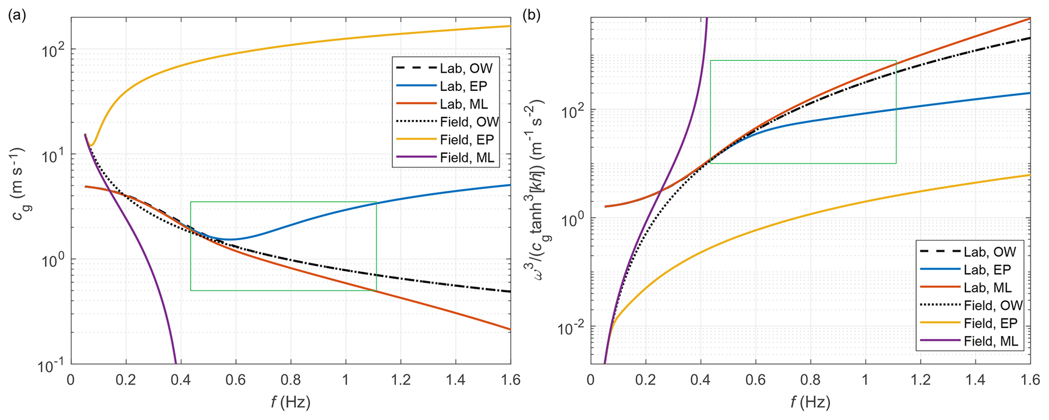
Figure 1Group velocity cg (a) and the ratio ω3∕(cgtanh 3[kh]) (b) versus wave frequency , computed for thin laboratory ice (test series 3000 from the LS-WICE experiment analysed in Part 2) and for field conditions with h=1000 m, ρw=1025 kg m−3, ρi=910 kg m−3, Pa, and hi=1.5 m. The corresponding open water solutions are shown in black (note that the two black curves overlap for f>0.5 Hz). Green rectangles mark regions covered by the LS-WICE experiment.
This very different behaviour of αc(ω) in the mass loading and elastic-plate models (originating from the group velocity decreasing or increasing with wave frequency, respectively; Fig. 1a) indicates that one should expect very different wave attenuation patterns related to ice–water drag in ice composed of small and large floes. Differences in the dispersion relation will lead to differences in attenuation rates, with very strong damping of high-frequency waves in fields of small ice floes (for which the mass loading model is a good approximation) and with roughly ω2–ω2.5 damping in continuous ice or fields of large ice floes. We return to this fact in the discussion section.
4.1 Model set-up
We set up the DEM for conditions corresponding to those from LS-WICE series 3000 (see Part 2). The ice sheet is 42 m long, and three floe lengths Lx are considered: 0.5 m (number of floes Nf=84), 1.5 m (Nf=28), and 3.0 m (Nf=14). For each floe size, the model is run for several different combinations of the following parameters: the wave period T (1.1, 1.2, 1.4, 1.5, 1.6, 1.8, and 2.0 s), incident wave amplitude a0 (0.0125, 0.015, 0.02, and 0.025 m), drag coefficient Csd (0.005, 0.01, 0.05, 0.1, 0.15, and 0.2), restitution coefficient ε (0.2, 0.4, 0.6, and 0.8), and initial floe–floe distance df (0.005, 0.010, 0.020, and 0.050 m). In each model run, the floes are initially placed along the x axis such that and for (tests with random initial locations of the floes have shown that this aspect of the set-up has no influence on the results). Additionally, for each value of T, three values of wavenumber k and group velocity cg were considered, computed from the EP, OW, and ML dispersion relations. Thus, the parameter space considered has seven dimensions.
As described in Part 2, the ice in LS-WICE was constrained horizontally by a floating boom and a sloping beach. In DEM, an analogous effect is obtained by adding a linear spring force Fs to the first and last floe, with for i=1 and i=Nf. The value of the spring constant ks was set to 9×10⁴ N m−1 (tests showed that the value of ks does not have visible results on the simulated attenuation, of interest in this study).
The time step Δt used in the simulations equaled s. In the algorithm (see Sect. 2.4), was used in the convergence criterion, with n0=10 and nT=5. The spatial resolution in numerical integration of dissipation, used in Eq. (19), was Δx=0.01 m.
As already mentioned, the analysis presented in the remaining parts of this paper concentrates on the role of ice–water drag; i.e. it is limited to results obtained without overwash, Sow=0. Simulations with overwash are discussed in Part 2.
4.2 Influence of the model parameters on simulated wave attenuation
We begin exploring the model behaviour with an analysis of the influence of the restitution coefficient ε on wave attenuation. Obviously, by definition of ε, the lower its value, the higher the fraction of kinetic energy of colliding objects that is dissipated during collisions. However, these energy losses, directly affecting the motion of the ice, do not automatically lead to the attenuation of the energy of the waves. On the contrary, as Fig. 2 clearly shows, the higher the ε, the lower the wave amplitude. The mechanism behind this relationship, described by Herman (2018) and mentioned in the Introduction, is related to enhanced relative ice–water velocities after collisions, leading to enhanced stress and thus stronger dissipation of wave energy.

Figure 2Computed relative wave amplitude a∕a0 for simulations with Lx=0.5 m, T=1.2 s, a0=0.0125 m, df=0.005 m, and Csd=0.05, with ML (a) and EP (b) dispersion relation. Colours correspond to different restitution coefficients ε; continuous black line shows the curve computed from Eq. (25), with αc from Eq. (24). Dots mark locations where the phase-averaged floe–floe distance drops below 10−4 m (see Fig. 3a), and black dashed lines originating from those points show corresponding solutions for compact ice.
Another aspect of the results immediately seen in Fig. 2 is that in most cases the slope of the a(x) curve changes with distance from the ice edge: da∕dx is large close to the ice edge, within a relatively narrow zone of very strong attenuation, and becomes smaller further down-wave. This effect is related to the rearrangement of the mean positions of the floes within the space available to them. As in every forced granular gas, the “atoms” tend to disperse from regions with higher granular pressure to regions where the granular pressure is lower. Thus, close to the ice edge, where collisions are more energetic due to stronger forcing (higher wave amplitudes), the local ice concentration becomes slightly lower and the floes accumulate further down-wave, in a densely packed zone of ice concentration close to 100 %, i.e. with floes in permanent contact with their neighbours (Fig. 3a). The width of the collisional zone at the ice edge decreases with increasing ε, and the above-mentioned change of slope of the a(x) curve corresponds to the location of the boundary between those two regions (see coloured dots in Figs. 2 and 3a). The two zones are, not surprisingly, characterized by different balance of forces. In the compact region with permanent floe–floe contact, the wave-induced forces are balanced by the contact forces, with drag force roughly 2 orders of magnitude lower (Fig. 3b–d); close to the ice edge, phase-averaged ice–water drag is still lower than the remaining forces, but it contributes a significantly larger part to the overall force balance. All these differences between the two regions are clearly seen in the time series of the energy dissipation term Ssd (Fig. 4). For floes close to the ice edge, large spikes in Ssd occur regularly after each collision. Floes far from the ice edge experience very low, periodically varying Ssd values related to small displacements from their average positions. Between those two regions of relatively regular – collisional or non-collisional – motion, the floes experience irregular fluctuations of their mean position (not shown) and associated periods with higher and lower collision rates, in effect producing erratic temporal patterns of Ssd (red curve in Fig. 4). Coming back to the wave attenuation, it is not surprising that the simulated attenuation rates in the down-wave high-concentration region are very close to those computed analytically for motionless ice (dashed lines in Fig. 2).
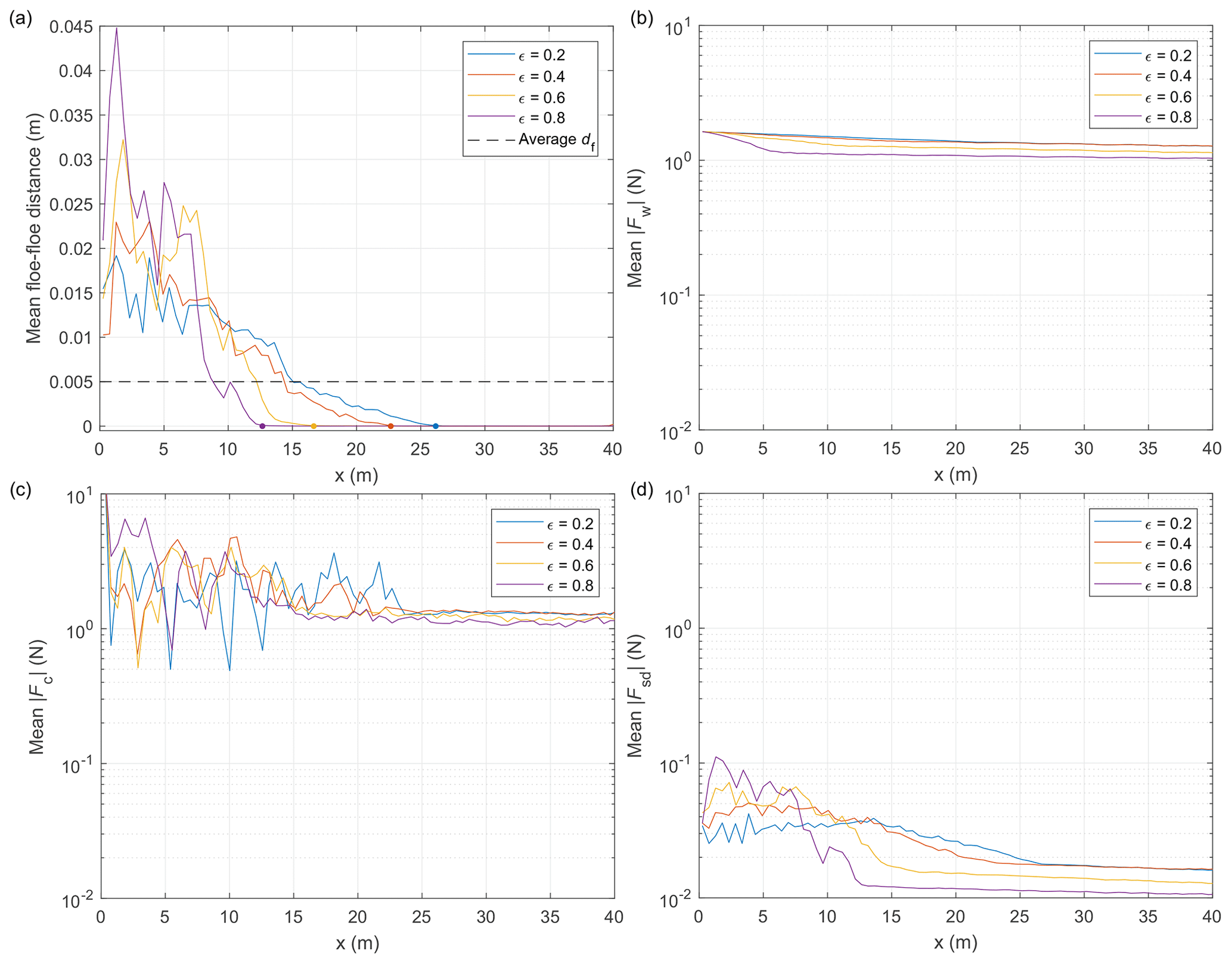
Figure 3Results of simulations with Lx=0.5 m, T=1.2 s, a0=0.0125 m, and df=0.005 m, with ML dispersion relation (as in Fig. 2a): mean floe–floe distance (a), mean (b), mean (c), and mean (d) for four values of restitution coefficient ε. In (a), black dashed line shows the domain average df, and dots mark locations where the average floe–floe distance drops below 10−4 m.
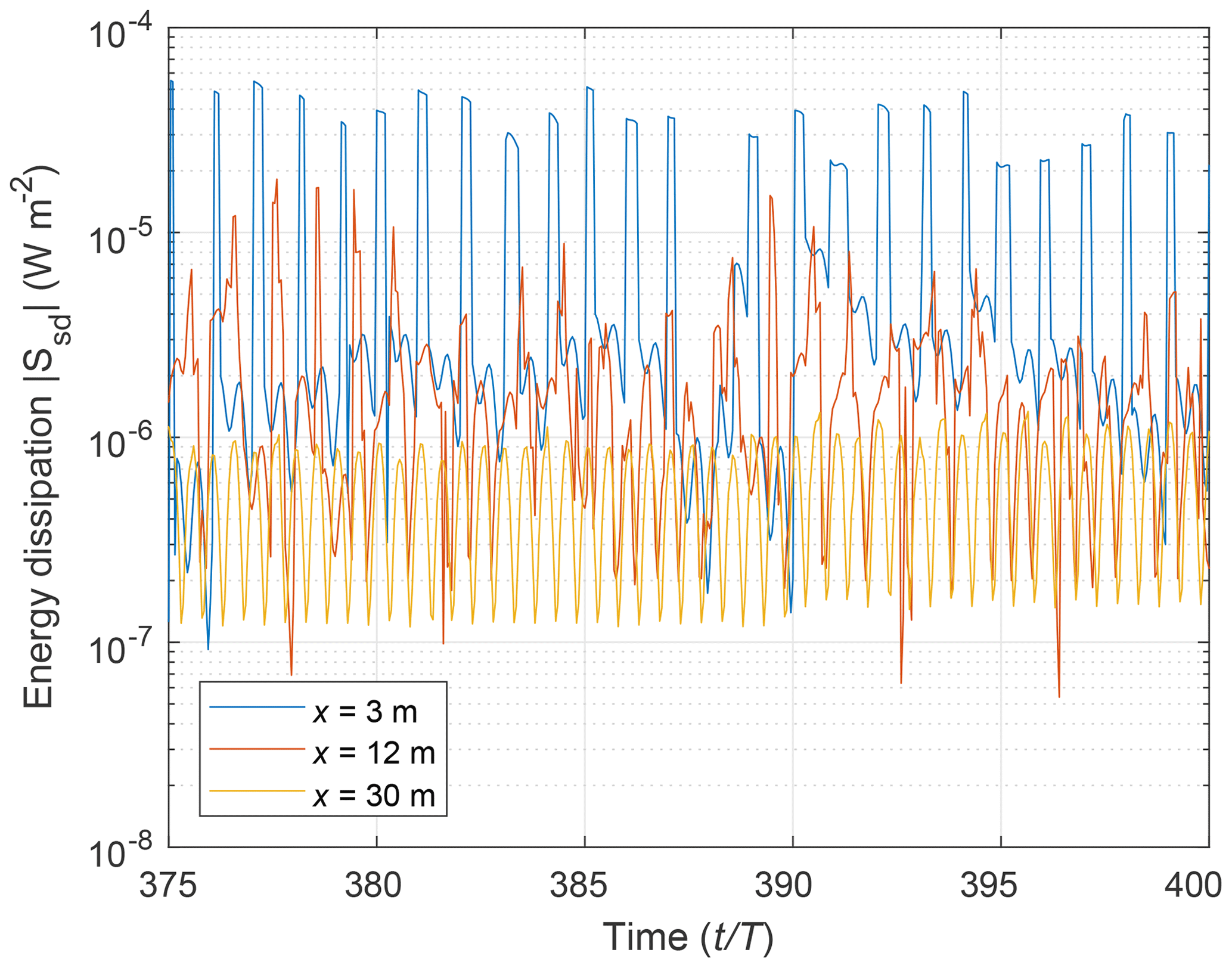
Figure 4Time series of the modulus of the wave energy dissipation term in simulations with Lx=0.5 m, T=1.2 s, a0=0.0125 m, Csd=0.05, ε=0.6, and ML dispersion relation (see yellow curve in Fig. 2a), for three selected floes, located at 3, 12, and 30 m from the ice edge.
It is also worth noting that the existence of the collisional zone at the ice edge, producing strong attenuation, is directly related to the fact that the ice edge position is fixed in space – by the boom in the laboratory and by the additional spring force in the model. Without that force, the floes drift gradually in the up-wave direction (again, towards lower granular pressure) until the ice concentration drops enough so that collisions become sporadic. We return to this issue in the discussion section.
As can be expected from the analysis in Sect. 2.3, the dispersion relation has a very strong influence on the simulated attenuation rates (compare Fig. 2a and b). With all other model parameters equal, the EP dispersion relation will always lead to lower attenuation rates than ML. Thus, at least two mechanisms contribute to stronger attenuation when ice floes are small. First, dispersion in ice fields composed of small floes is better described by the ML than by the EP model. And, second, small floes undergo more vigorous collisions, with larger instantaneous accelerations and more collisions per distance travelled by the wave. In an example shown in Fig. 5, the ML model is likely more suitable for small floes with Lx=0.5 m, and the EP model is more suitable for large floes with Lx=3.0 m, so that the expected difference in attenuation observed in these two situations can be as large as between the dashed yellow and the continuous blue line in Fig. 5.
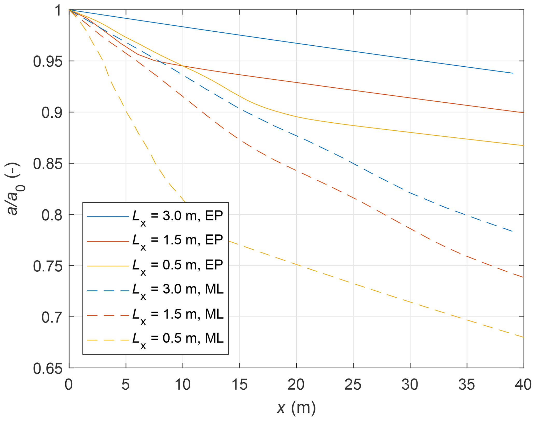
Figure 5Computed relative wave amplitude a∕a0 for simulations with different floe sizes Lx (colours), with T=1.4 s, a0=0.015 m, df=0.005 m, Csd=0.05, and ε=0.6, with EP (continuous lines) and ML (dashed lines) dispersion relation.
The fact that the frequency and character of collisions play a crucial role in shaping floe dynamics and wave energy dissipation in the region close to the ice edge means that the ice concentration, and thus the floe–floe distances, should have a visible influence on attenuation. This is indeed the case (Fig. 6a): when df decreases, attenuation increases. However, as can be seen for the results with short waves, stronger attenuation close to the ice edge means that the zone of strong attenuation becomes narrower so that further down-wave, the relationship between df and a∕a0 reverses (in Fig. 6a, no analogous effect is present for the longer waves with T=1.8 s because the collisional zone extends in this case over the whole model domain). Those examples illustrate how difficult it might be to “reconstruct” the attenuation curves from measurements available only at a limited number of locations (as in the case discussed in Part 2) and how careful one should be when interpreting those kinds of data.
Finally, it is worth stressing that the modelled wave attenuation in both regions is strongly dependent on the incident wave amplitude a0 (Fig. 6b). In the collisional zone at the ice edge, the wave amplitude decides on the surge amplitude of the floes and thus on the occurrence and intensity of collisions. Further down-wave, the a(x) curve is described well by Eq. (25); i.e. the attenuation rate is close to a0αc.
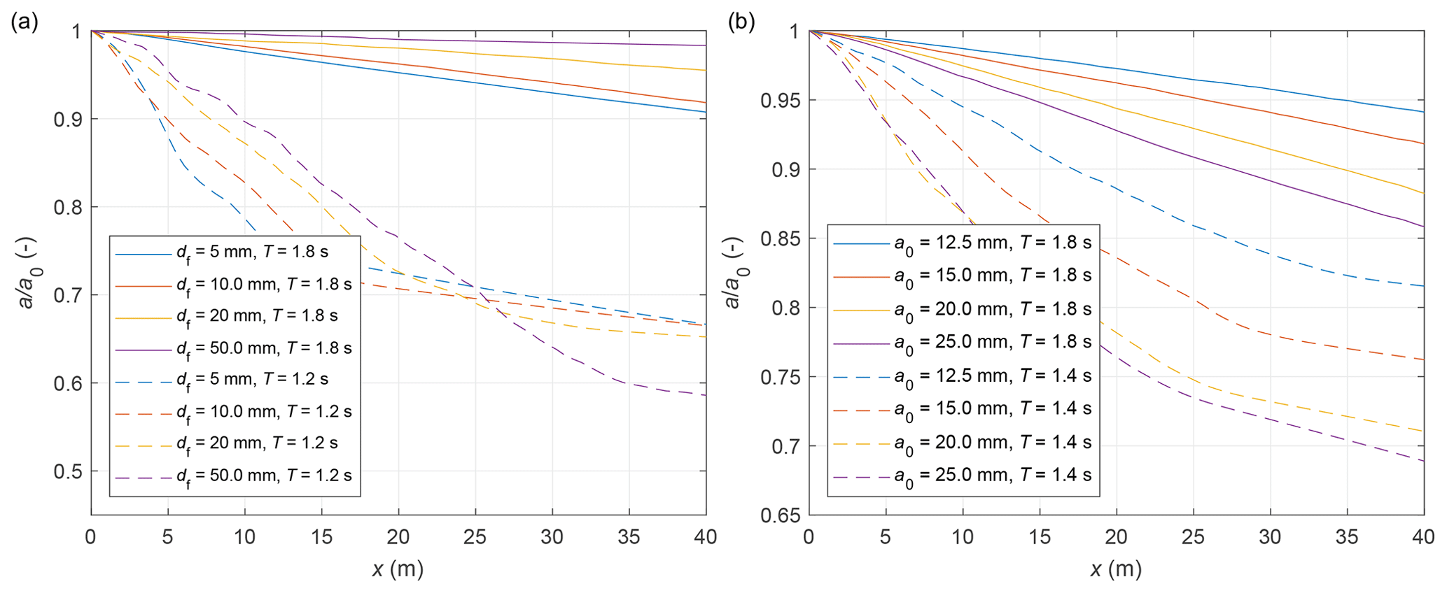
Figure 6Computed relative wave amplitude a∕a0 for simulations with different average floe–floe distance df (a) and different incident wave amplitude a0 (b), for Lx=0.5 m, a0=0.015 m, df=0.005 m, Csd=0.05, and ε=0.6, for two different wave periods.
As noted recently by Meylan et al. (2018), the dependence of the attenuation rate α on wave frequency follows directly from the formulation of a given model, and therefore – if the model does not properly reproduce the relevant processes – its coefficients can be tuned to the observed attenuation at one frequency only. Reversing this argument, the observed functional forms of a(x) and α(f) can be treated as signatures of physical attenuation processes that have shaped them. It is thus crucial to improve our understanding of how different attenuation mechanisms influence a(x) and α(f). In this work, we concentrated on one of those mechanisms: dissipation of wave energy due to ice–water drag. We used DEM simulations and, in a limiting case of compact sea ice, an analytical analysis, in order to investigate how ice–water drag influences the dynamics of sea ice floes and the corresponding attenuation of wave energy. Several aspects of the results, mentioned in the text, are worth further discussion.
The DEM simulations predict a very distinctive pattern of wave attenuation resulting from combined effects of ice–water drag and collisions between ice floes. The results suggest that intense collisions between ice floes can be expected to occur only within a narrow zone close to the ice edge, which is also a zone of lowered ice concentration and of very strong attenuation – provided that the floes are not able to drift in the up-wave direction. In natural conditions, forces keeping the ice edge in place may include compressive stress caused by wave reflection from the ice edge as well as wind and/or average currents with sufficient velocity so that the forces exerted by them on the ice compensate for those related to increased granular pressure. It is interesting to note that the elevated granular pressure can be sustained only by a constant energy input from the waves; otherwise, inelastic floe–floe collisions would lead not to increased, but to decreased, collision rates. This makes the situation very different from the wind-forced sea ice studied by Herman (2011, 2012), where floes tended to accumulate in regions of intense collisions, producing clusters with high ice concentration. In the present case, thanks to the interplay with wave forcing, the same basic mechanisms lead to the formation of the two zones described in Sect. 4.2, with very different wave attenuation rates and collision patterns. Notably, also, if the ice floes are small relative to the wavelength, very different attenuation should be expected in situations with a confined ice edge (strong ice–water drag due to floe collisions at high ice concentration) and in situations with a “free” ice edge (no collisions due to lowered ice concentration or floes able to follow the motion of the water).
The fact that the floes tend to accumulate in the inner zone, forming a semi-continuous ice cover with ice concentration close to 100 % and limited horizontal ice motion, means that – if dissipation due to ice–water drag is significant – the expected attenuation rates within that zone should be close to those computed analytically in Sect. 3. From a practical point of view, it substantially simplifies the situation, eliminating, from the set of relevant variables, the variables related to collisions. Crucially, as illustrated in Sect. 3, the behaviour of α(ω) in this case depends very strongly on the dispersion relation, with much weaker dissipation in sea ice composed of large ice floes, behaving as elastic plates, and stronger dissipation in sea ice composed of small floes, behaving as rigid “mass points”. It must be stressed here that the strong influence of the dispersion relation on α(ω) is not limited to the dissipation mechanisms discussed in this paper. As the left-hand side of Eq. (9) has the form d(cgEw)∕dx, the value of will always influence the energy attenuation, contributing to stronger attenuation in small floes (when cg is relatively low and decreases with increasing wave frequency) than in large floes (when cg is larger and increases with increasing frequency; Fig. 1a). In many studies these effects are not taken into account and open-water dispersion relation is assumed (e.g. Meylan et al., 2018), although several observations, including those analysed by Liu and Mollo-Christensen (1988) or Sutherland and Rabault (2016), show the influence of floe size on wave propagation speed (in the LS-WICE experiment discussed in Part 2, for which the present DEM was configured, decreasing wavenumbers with increasing floe size were observed, as analysed by Cheng et al., 2018). The example of attenuation due to ice–water drag, discussed in this work, suggests that even small changes of cg may lead to noticeable changes of α. In the inner zone far from the ice edge, where the floes tend to be larger and therefore α should be close to αc,ep, the present model predicts a power-law tail in the relation α(ω), with the power m typically between 2 and 2.5 depending on ice properties, i.e. substantially lower than m=4 for the open water dispersion relation. This is a very important aspect of our results, as the values 2–2.5 are in agreement with many observations, although, obviously, it does not mean that the analysed mechanism significantly contributes to attenuation in real sea ice.
It is also worth noting that the influence of ice–water drag on wave energy attenuation depends very strongly on the drag law used. If, for example, a linear drag law τw∼urel is used instead of the quadratic law (Eq. 15), exponential attenuation is obtained instead of Eq. (25), with αc,l proportional to ω2∕(cgtanh 2[kh]); i.e. the increase in the attenuation coefficient αc,l with ω is slower than predicted by the model described earlier. This illustrates that both the shape of the attenuation curve a(x) and the attenuation coefficients are very sensitive to the formulation of the dissipation term in the energy transport equation (Eq. 9). On the other hand, any model with a dissipative force quadratically dependent on relative ice–water velocity will exhibit a similar behaviour. For example, replacing the drag coefficient Csd, here representing skin drag, with a form drag coefficient, and replacing integration over the bottom surface of the floes in Eq. (13) with integration over their vertical walls, should not change the general attenuation behaviour described above.
A very important limitation of the model used here is the fact that it takes into account only the transmitted propagating component (T0 in the notation of Kohout et al., 2007) of the wave motion. As our analysis in Part 2 shows, the contribution of T0 to the total wave amplitude in the LS-WICE experiment is variable and strongly dependent on the ratio of floe size to wavelength. From the point of view of the ice–water drag, discussed in this paper, it is important to keep in mind that the additional modes – especially the propagating damped modes (T−2, T−1, R−2, and R−1), which might have amplitudes comparable with T0 – modify the spatial and temporal variability in uw, thus modifying the instantaneous and phase-averaged urel and Ssd. It remains to be investigated how large those changes might be in different conditions. Moreover, the damped modes increase the water velocities close to the edges of the floes as well as the amplitude of the vertical motion of floes' edges (the total amplitude is a sum of the amplitude of the propagating components, constant over the length of the floe, and the amplitude of the damped components, decreasing from floe edges towards its inner parts). Thus, the presence of the damped modes might modify overwash and, combined with floe collisions, contribute to the enhancement of turbulent mixing at floe boundaries. Although analysing interrelationships between those processes in full detail will require much more advanced models and observations, an initial step in that direction can be done by extending the present DEM so that more realistic wave forcing can be used. The same is true with another limitation of this study – the fact that both the DEM and the laboratory set-up discussed in Part 2 are one-dimensional. Estimating the strength of additional effects in situations with directional wave energy spectra and fully two-dimensional floe–floe collisions, scattering, etc., is extremely difficult based on the present one-dimensional simulations and would require extending the existing coupled model to two dimensions.
The code of the DESIgn model is freely available at https://herman.ocean.ug.edu.pl/LIGGGHTSseaice.html (last access: 7 November 2019) and as a Supplement to Herman (2016). The extended code necessary to reproduce the results presented in this paper, together with input scripts, can be obtained from the corresponding author.
All authors contributed to the planning of the research and to the discussion of the results. AH developed the numerical model, performed the simulations, and wrote the text.
The authors declare that they have no conflict of interest.
We are very grateful to the two anonymous reviewers for very insightful and constructive comments on the draft of this paper.
The development of the numerical model used in this work has been financed by the Polish National Science Centre research grant no. 2015/19/B/ST10/01568 (“Discrete-element sea ice modeling – development of theoretical and numerical methods”). Sukun Cheng and Hayley H. Shen are supported in part by ONR grant no. N00014-17-1-2862.
This paper was edited by Lars Kaleschke and reviewed by two anonymous referees.
Ardhuin, F., Collard, F., Chapron, B., Girard-Ardhuin, F., Guitton, G., Mouche, A., and Stopa, J.: Estimates of ocean wave heights and attenuation in sea ice using the SAR wave mode on Sentinel-1A, Geophys. Res. Lett., 42, 2317–2325, https://doi.org/10.1002/2014GL062940, 2015. a
Ardhuin, F., Boutin, G., Stopa, J., Girard-Ardhuin, F., Melsheimer, C., Thomson, J., Kohout, A., Doble, M., and Wadhams, P.: Wave attenuation through an arctic marginal ice zone on 12 October 2015: 2. Numerical modeling of waves and associated ice breakup, J. Geophys. Res., 123, 5652–5668, https://doi.org/10.1002/2018JC013784, 2018. a
Bateson, A. W., Feltham, D. L., Schröder, D., Hosekova, L., Ridley, J. K., and Aksenov, Y.: Impact of floe size distribution on seasonal fragmentation and melt of Arctic sea ice, The Cryosphere Discuss., https://doi.org/10.5194/tc-2019-44, in review, 2019. a
Bennetts, L. and Squire, V.: Model sensitivity analysis of scattering-induced attenuation of ice-coupled waves, Ocean Model., 45–46, 1–13, https://doi.org/10.1016/j.ocemod.2012.01.002, 2012. a
Cheng, S., Rogers, W., Thomson, J., Smith, M., Doble, M., Wadhams, P., Kohout, A., Lund, B., Persson, O., Collins III, C., Ackley, S., Montiel, F., and Shen, H.: Calibrating a viscoelastic sea ice model for wave propagation in the Arctic fall marginal ice zone, J. Geophys. Res., 122, 8740–8793, https://doi.org/10.1002/2017JC013275, 2017a. a
Cheng, S., Tsarau, A., Li, H., Herman, A., Evers, K.-U., and Shen, H.: Loads on Structure and Waves in Ice (LS-WICE) project, Part 1: Wave attenuation and dispersion in broken ice fields, in: Proc. 24th Int. Conf. on Port and Ocean Engineering under Arctic Conditions (POAC), Busan, Korea, 11–16 June, 2017b. a
Cheng, S., Tsarau, A., Evers, K.-U., and Shen, H.: Floe size effect on gravity wave propagation through ice covers, J. Geophys. Res., 124, 320–334, https://doi.org/10.1029/2018JC014094, 2018. a, b, c
Collins, C., Rogers, W., and Lund, B.: An investigation into the dispersion of ocean surface waves in sea ice, Ocean Dynam., 67, 263–280, https://doi.org/10.1007/s10236-016-1021-4, 2017. a
De Santi, F., De Carolis, G., Olla, P., Doble, M., Cheng, S., Shen, H., Wadhams, P., and Thomson, J.: On the Ocean wave attenuation rate in grease-pancake ice, a comparison of viscous layer propagation models with field data, J. Geophys. Res., 123, 5933–5948, https://doi.org/10.1029/2018JC013865, 2018. a
Doble, M., De Carolis, G., Meylan, M., Bidlot, J.-R., and Wadhams, P.: Relating wave attenuation to pancake ice thickness, using field measurements and model results, Geophys. Res. Lett., 42, 4473–4481, https://doi.org/10.1002/2015GL063628, 2015. a
Fox, C. and Squire, V.: Reflection and transmission characteristics at the edge of shore fast sea ice, J. Geophys. Res., 95, 11629–11639, https://doi.org/10.1029/JC095iC07p11629, 1990. a
Hayes, D., Jenkins, A., and McPhail, S.: Autonomous underwater vehicle measurements of surface wave decay and directional spectra in the marginal sea ice zone, J. Phys. Oceanogr., 37, 71–83, https://doi.org/10.1175/JPO2979.1, 2007. a
Herman, A.: Molecular-dynamics simulation of clustering processes in sea-ice floes, Phys. Rev. E, 84, 056104, https://doi.org/10.1103/PhysRevE.84.056104, 2011. a
Herman, A.: Influence of ice concentration and floe-size distribution on cluster formation in sea ice floes, Cent. Europ. J. Phys., 10, 715–722, https://doi.org/10.2478/s11534-012-0071-6, 2012. a
Herman, A.: Discrete-Element bonded-particle Sea Ice model DESIgn, version 1.3a – model description and implementation, Geosci. Model Dev., 9, 1219–1241, https://doi.org/10.5194/gmd-9-1219-2016, 2016. a, b
Herman, A.: Wave-induced surge motion and collisions of sea ice floes: finite-floe-fize effects, J. Geophys. Res., 123, 7472–7494, https://doi.org/10.1029/2018JC014500, 2018. a, b, c, d, e, f, g, h, i
Herman, A., Cheng, S., and Shen, H. H.: Wave energy attenuation in fields of colliding ice floes – Part 2: A laboratory case study, The Cryosphere, 13, 2901–2914, https://doi.org/10.5194/tc-13-2901-2019, 2019. a
Kohout, A.: Water wave scattering by floating elastic plates with application to sea-ice, PhD thesis, Univ. of Auckland, New Zealand, 188 pp., 2008. a
Kohout, A. and Meylan, M.: An elastic plate model for wave attenuation and ice floe breaking in the marginal ice zone, J. Geophys. Res., 113, C09016, https://doi.org/10.1029/2007JC004434, 2008. a, b, c
Kohout, A., Meylan, M., Sakai, S., Hanai, K., Leman, P., and Brossard, D.: Linear water wave propagation through multiple floating elastic plates of variable properties, J. Fluids Structures, 23, 649–663, https://doi.org/10.1016/j.jfluidstructs.2006.10.012, 2007. a
Kohout, A., Meylan, M., and Plew, D.: Wave attenuation in a marginal ice zone due to the bottom roughness of ice floes, Ann. Glaciol., 52, 118–122, 2011. a, b
Li, J., Kohout, A., and Shen, H.: Comparison of wave propagation through ice covers in calm and storm conditions, Geophys. Res. Lett., 42, 5935–5941, https://doi.org/10.1002/2015GL064715, 2015. a
Liu, A. and Mollo-Christensen, E.: Wave propagation in a solid ice pack, J. Phys. Oceanogr., 18, 1702–1712, 1988. a, b
Liu, A., Holt, B., and Vachon, P.: Wave propagation in the marginal ice zone: Model predictions and comparisons with buoy and synthetic aperture radar data, J. Geophys. Res., 96, 4605–4621, https://doi.org/10.1029/90JC02267, 1991. a, b
Meylan, M., Bennetts, L., and Kohout, A.: In situ measurements and analysis of ocean waves in the Antarctic marginal ice zone, Geophys. Res. Lett., 41, 5046–5051, https://doi.org/10.1002/2014GL060809, 2014. a
Meylan, M., Bennetts, L., Mosig, J., Rogers, W., Doble, M., and Peter, M.: Dispersion relations, power laws, and energy loss for waves in the marginal ice zone, J. Geophys. Res., 123, 3322–3335, https://doi.org/10.1002/2018JC013776, 2018. a, b, c
Montiel, F. and Squire, V.: Modelling wave-induced sea ice breakup in the marginal ice zone, Proc. R. Soc. A, 473, 20170258, https://doi.org/10.1098/rspa.2017.0258, 2017. a
Montiel, F., Squire, V., and Bennetts, L.: Attenuation and directional spreading of ocean wave spectra in the marginal ice zone, J. Fluid Mech., 790, 492–522, https://doi.org/10.1017/jfm.2016.21, 2016. a
Montiel, F., Squire, V., Doble, M., Thomson, J., and Wadhams, P.: Attenuation and directional spreading of ocean waves during a storm event in the autumn Beaufort Sea marginal ice zone, J. Geophys. Res., 123, 5912–5932, https://doi.org/10.1029/2018JC013763, 2018. a
Rogers, W., Thomson, J., Shen, H., Doble, M., Wadhams, P., and Cheng, S.: Dissipation of wind waves by pancake and frazil ice in the autumn Beaufort Sea, J. Geophys. Res., 121, 7991–8007, https://doi.org/10.1002/2016JC012251, 2016. a, b
Shen, H. and Squire, V.: Wave damping in compact pancake ice fields due to interactions between pancakes, in: Antarctic Sea Ice: Physical Processes, Interactions and Variability, 74, 325–341, 1998. a, b, c, d, e
Skene, D., Bennetts, L., Meylan, M., and Toffoli, A.: Modelling water wave overwash of a thin floating plate, J. Fluid Mech., 777, R3, https://doi.org/10.1017/jfm.2015.378, 2015. a, b, c
Skene, D., Bennetts, L., Wright, M., and Meylan, M.: Water wave overwash of a step, J. Fluid Mech., 839, 293–312, https://doi.org/10.1017/jfm.2017.857, 2018. a, b, c
Squire, V.: Of ocean waves and sea-ice revisited, Cold Reg. Sci. Technol., 49, 110–133, 2007. a
Squire, V.: A fresh look at how ocean waves and sea ice interact, Phil. Trans. R. Soc. A, 376, 20170342, https://doi.org/10.1098/rsta.2017.0342, 2018. a, b
Squire, V. and Montiel, F.: Evolution of directional wave spectra in the marginal ice zone: a new model tested with legacy data, J. Phys. Oceanogr., 46, 3121–3137, https://doi.org/10.1175/JPO-D-16-0118.1, 2016. a
Stopa, J., Ardhuin, F., Thomson, J., Smith, M., Kohout, A., Doble, M., and Wadhams, P.: Wave attenuation through an Arctic marginal ice zone on 12 October 2015. 1. Measurement of wave spectra and ice features from Sentinel 1A, J. Geophys. Res., 123, 3619–3634, https://doi.org/10.1029/2018JC013791, 2018a. a, b
Stopa, J., Sutherland, P., and Ardhuin, F.: Strong and highly variable push of ocean waves on Southern Ocean sea ice, P. Natl. Acad. Sci. USA, 115, 5861–5865, https://doi.org/10.1073/pnas.1802011115, 2018b. a, b
Sutherland, G. and Rabault, J.: Observations of wave dispersion and attenuation in landfast ice, J. Geophys. Res., 121, 1984–1997, https://doi.org/10.1002/2015JC011446, 2016. a
Sutherland, G., Christensen, K., Rabault, J., and Jensen, A.: A new look at wave dissipation in the marginal ice zone, arXiv:1805.01134, 2018a. a
Sutherland, P. and Dumont, D.: Marginal ice zone thickness and extent due to wave radiation stress, J. Phys. Oceanogr., 48, 1885–1901, https://doi.org/10.1175/JPO-D-17-0167.1, 2018. a
Sutherland, P., Brozena, J., Rogers, W., Doble, M., and Wadhams, P.: Airborne remote sensing of wave propagation in the marginal ice zone, J. Geophys. Res., 123, 4132–4152, https://doi.org/10.1029/2018JC013785, 2018b. a
Wadhams, P., Squire, V., Goodman, D., Cowan, A., and Moore, S.: The attenuation rates of ocean waves in the marginal ice zone, J. Geophys. Res., 93, 6799–6818, https://doi.org/10.1029/JC093iC06p06799, 1988. a