the Creative Commons Attribution 4.0 License.
the Creative Commons Attribution 4.0 License.
 | 14 Jan 2019
New insight from CryoSat-2 sea ice thickness for sea ice modelling
David Schröder
Danny L. Feltham
Michel Tsamados
Andy Ridout
Rachel Tilling
Estimates of Arctic sea ice thickness have been available from the CryoSat-2 (CS2) radar altimetry mission during ice growth seasons since 2010. We derive the sub-grid-scale ice thickness distribution (ITD) with respect to five ice thickness categories used in a sea ice component (Community Ice CodE, CICE) of climate simulations. This allows us to initialize the ITD in stand-alone simulations with CICE and to verify the simulated cycle of ice thickness. We find that a default CICE simulation strongly underestimates ice thickness, despite reproducing the inter-annual variability of summer sea ice extent. We can identify the underestimation of winter ice growth as being responsible and show that increasing the ice conductive flux for lower temperatures (bubbly brine scheme) and accounting for the loss of drifting snow results in the simulated sea ice growth being more realistic. Sensitivity studies provide insight into the impact of initial and atmospheric conditions and, thus, on the role of positive and negative feedback processes. During summer, atmospheric conditions are responsible for 50 % of September sea ice thickness variability through the positive sea ice and melt pond albedo feedback. However, atmospheric winter conditions have little impact on winter ice growth due to the dominating negative conductive feedback process: the thinner the ice and snow in autumn, the stronger the ice growth in winter. We conclude that the fate of Arctic summer sea ice is largely controlled by atmospheric conditions during the melting season rather than by winter temperature. Our optimal model configuration does not only improve the simulated sea ice thickness, but also summer sea ice concentration, melt pond fraction, and length of the melt season. It is the first time CS2 sea ice thickness data have been applied successfully to improve sea ice model physics.
- Article
(5715 KB) - Full-text XML
- BibTeX
- EndNote


Historical observations of sea ice thickness have been limited due to their sparse spatial and temporal coverage of, and uncertainties in, measurements. Prior to the launch of the European Space Agency's (ESA) first European Remote Sensing satellite (ERS-1) in 1991, most data were collected from submarines operating beneath the Arctic pack ice. Upward-looking sonars measure the submerged portion of the ice (draft), which can be converted to thickness by making assumptions about the snow depth and the densities of ice, snow, and water. Based on sea ice draft observations from 34 US Navy submarines, a decrease of mean autumn sea ice thickness from 2.8 to 1.6 m could be identified over the period 1975–2000 within the central Arctic Ocean (Rothrock et al., 2008). While the accuracy and the spatial coverage were sufficient to give evidence of sea ice thinning in the Arctic and to provide a basis for simulating the trend, these data are of limited use for evaluating the spatial and temporal variability of sea ice across the Arctic, and in climate models. More recently, cryosphere-focused satellite altimeters such as the NASA Ice, Cloud, and land Elevation Satellite (ICESat) and ESA CryoSat-2 (CS2) have allowed estimation of sea ice thickness across the Arctic (Giles et al., 2007, 2008; Kwok and Rothrock, 2009; Laxon et al., 2013).
The performance of sea ice models in climate models is most commonly evaluated by using Arctic- and Antarctic-wide sea ice extent and sea ice area data from passive microwave data and Arctic sea ice volume from the Pan-Arctic Ice Ocean Modeling and Assimilation System (PIOMAS; Zhang and Rothrock, 2003; e.g. Massonnet et al., 2012; Stroeve et al., 2012; Rae et al., 2014; Shu et al., 2015; Ridley et al., 2018). PIOMAS is a reanalysis product, which does not include ice thickness observations. Stroeve et al. (2014) combined submarine, aircraft, and satellite data to evaluate sea ice thickness in climate model simulations. Their assessment revealed shortcomings regarding spatial patterns of sea ice thickness that were larger than uncertainties in the verification data. CS2 sea ice thickness data have recently been used to initialize sea ice ocean and climate models to improve seasonal predictions (Allard et al., 2018; Blockley and Peterson, 2018).
In this study, we aim to improve sea ice physics and to calibrate poorly constrained parameters in the sea ice model CICE (Community Ice CodE) using the CS2 ice thickness data. Given that CS data are available from October to April, our focus lies on processes controlling winter ice growth. We note that several factors contribute to CS2-derived sea ice thickness uncertainties, including the assumption that the radar return is from the snow–ice interface (Willat et al., 2011), snow depth departures from climatology, and the use of fixed snow and ice densities. To enable a meaningful comparison of sea ice thickness between CICE and CS2, we consider the strengths and weaknesses of the model and the data. We design experiments with perturbed physical parameterizations to close the gap between our default CICE simulation and CS2 as well as to investigate the impact of initial conditions and atmospheric forcing data. The latter experiments address questions regarding the impact of the last three exceptionally warm Arctic winters on the sea ice decline (Stroeve et al., 2018) and give new insight into the strengths of positive and negative feedback mechanisms that govern the evolution of sea ice.
The CS2 radar altimetry mission was launched in April 2010, providing estimates of ice thickness during the ice growth season from October to April. During summer the formation of melt ponds interferes with the radar signal, retarding accurate measurements. As for the derivation of sea ice thickness from the ice draft using submarine data, the freeboard (the height of sea ice above the water surface) is estimated from the satellite data and can be converted to thickness by assuming hydrostatic equilibrium and applying values for the densities of ice, snow, and water as well as the snow depth. The principal challenges in deriving an accurate sea ice thickness using satellite altimetry are the discrimination of ice and open water, the discrimination of ice type, the retracking of radar waveforms to obtain height estimates, the construction of sea surface height beneath the ice, and estimation of the depth of the snow cover. Ice thickness is retrieved from the freeboard by processing CS2 Level 1B data, with a footprint of approximately 300 m × 1700 m (Wingham et al., 2006), and assuming snow density and snow depth from the Warren et al. (1999) climatology (hereafter W99), modified for the distribution of multi-year versus first-year ice (see Laxon et al., 2013, and Tilling et al., 2018, for data processing details).
In this study, we bin the individual thickness point measurements provided by the Centre for Polar Observation and Modelling (CPOM) into five CICE thickness categories, (1) ice thickness h<0.6 m, (2) 0.6 m m, (3) 1.4 m m, (4) 2.4 m m, and (5) h>3.6 m, on a rectangular 50 km grid for each month. The mean area fraction and mean thickness are derived for each thickness category and these values are interpolated on the ORCA tripolar 1∘ grid used by CICE (∼ 40 km grid resolution). Tilling et al. (2018) derived a general grid cell ice thickness uncertainty of 25 %. Grid cells with fewer than 100 individual measurements and a grid cell mean sea ice thickness of less than 0.5 m are omitted due to their increased uncertainty (Ricker et al., 2017). Otherwise, the whole range of individual observations from applied grid points are included. Negative thickness values are retained in the CS2 processing to prevent statistical positive bias of the thinner ice and are added to category 1. This approach allows us to initialize the CICE model with the full ice thickness distribution (ITD) rather than to derive the ITD from the mean sea ice thickness (Hunke et al., 2015). A realistic ITD is critical for simulating ice growth and ice melt rates correctly: given the identical mean ice thickness, a wider distribution leads to an increase of ice growth in winter because ice growth mainly takes place over the thinner ice, whereas during summer, the thinner ice melting away increases the lead fraction, resulting in a warmer ocean mixed-layer temperature, thus accelerating the sea ice melt.
In addition to CPOM CS2, we include sea ice thickness data provided by the Alfred Wegener Institute (AWI; Hendricks et al., 2016) and the National Aeronautics and Space Administration (NASA; Kurtz and Harbeck, 2017). The comparison of the three CS2 data sets illustrates a part of their uncertainty and helps us to assess the robustness of model–CS2 ice thickness differences. While all three data providers rely on W99 for snow depth and density, there is variation in how it is applied. CPOM spatially averages the W99 snow depth and then halves it over first-year ice (Tilling et al., 2018); AWI and NASA also halve W99 snow depth over first-year ice but discard measurements in lower latitude regions (Ricker et al., 2014; Hendricks et al., 2016; Kurtz et al., 2013). Each institution also processes the radar returns differently. When estimating ice freeboard, the range to the main scattering horizon of the radar return is obtained using a retracker algorithm. CPOM uses a Gaussian-exponential retracker for ocean waveforms and a threshold first maximum retracker algorithm (TFMRA) with a 70 % threshold for sea ice waveforms (Tilling et al., 2018), AWI applies a 50 % TFMRA to all waveforms (Ricker et al., 2014; Hendricks et al., 2016), and the NASA estimates rely on a physical model to best fit each waveform (Kurtz et al., 2014; Kurtz and Harbeck, 2017). This could lead to ice thickness differences based on different retrackers and thresholds applied.
CS2 ice thickness data for October appear to be less robust as indicated by large differences between the three products for thin first-year ice (not shown) and by large differences in comparison with ESA's Soil Moisture and Ocean Salinity (SMOS) sea ice data (Wang et al., 2016), so we only include CS data from November to April in our study.
3.1 Set-up
CICE is a dynamic–thermodynamic sea ice model designed for inclusion within a global climate model. The sea ice velocity is calculated from a momentum balance equation that accounts for air drag, ocean drag, Coriolis force, sea surface tilt, and the internal ice stress. The CICE model solves one-dimensional vertical heat balance equations for each ice thickness category. See Hunke et al. (2015) for a detailed description of the CICE model. Here, we perform stand-alone (fully forced) CICE simulations with version 5.1.2 for a pan-Arctic region (∼ 40 km grid resolution). CICE contains a simple mixed-layer ocean model with a prognostic ocean temperature. To account for heat transport in the ocean, we restore the mixed-layer ocean temperature and salinity to climatological monthly means from MYO-WP4-PUM-GLOBAL-REANALYSIS-PHYS-001-004 (Ferry et al., 2011) with a restoring timescale of 20 days. We apply a climatological ocean current (monthly means) from the same ocean reanalysis product. NCEP Reanalysis-2 (NCEP2) atmospheric reanalysis data (Kanamitsu et al., 2002, updated 2017) are used as atmospheric forcing. We perform a multi-year simulation from 1980 to 2017 which does not utilize CS2 ice thickness data (referred to as CICE-free) and seven 1-year-long simulations which are initialized with CS2 ice thickness data (referred to as CICE-ini) starting in mid-November and running until the end of November of the following year for the seven winter periods from 2010/11 to 2016/17. The initial thickness and concentration for each of the five ice categories are taken from the CPOM CS2 ITD November mean thickness fields. For grid points without CS2 data, and for all other variables (e.g. temperature profiles, snow volume), results from the free CICE simulation are applied. In this way, CICE simulations cover the pan-Arctic region, but in regions where no CS2 data are available, we restart with ice thickness values from the free CICE model run. While this approach would be problematic in a coupled model, in a stand-alone sea ice simulation, the model adjustment to the new conditions is smooth and the impact of using the vertical temperature profile from the free simulation only affects sea ice thickness on the order of millimetres.
3.2 Reference simulation (CICE-default)
Our reference simulation includes a prognostic melt pond model (Flocco et al., 2010, 2012) and the elastic anisotropic plastic rheology (Wilchinski and Feltham, 2006; Tsamados et al., 2013; Heorton et al., 2018). Otherwise, default CICE settings are chosen: seven vertical ice layers, one snow layer, linear remapping ITD approximation (Lipscomp and Hunke, 2004), Bitz and Libscomp (1999) thermodynamics, Maykut and Untersteiner (1971) conductivity, the Rothrock (1975) ridging scheme with a Cf value of 12 (empirical parameter that accounts for frictional energy dissipation), and the delta-Eddington radiation scheme (Briegleb and Light, 2007).
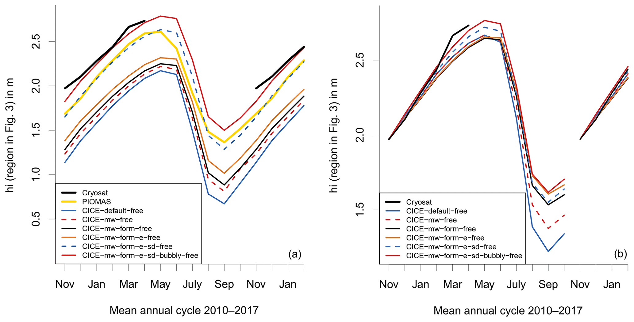
Figure 1Impact of CICE set-up on mean effective sea ice thickness over the region shown in Fig. 3 and averaged over winter periods 2010/11 to 2016/17: (a) CICE-free simulations (multi-year runs from 1980 to 2017) and (b) CICE-ini simulations (seven 1-year-long runs starting in mid-November with CS2 sea ice thickness). Model results are compared with mean sea ice thickness from CS2 CPOM and PIOMAS. Effective ice thickness (divided by ice concentration) is presented. For CS2 ice concentration is applied from CICE-default (mean values for November to April vary between 99.4 % and 99.8 %). See Sect. 3.3.1 for explanation of CICE % experiments. Note that results for November, December, January, and February are shown twice for improved visualization of the annual cycle.
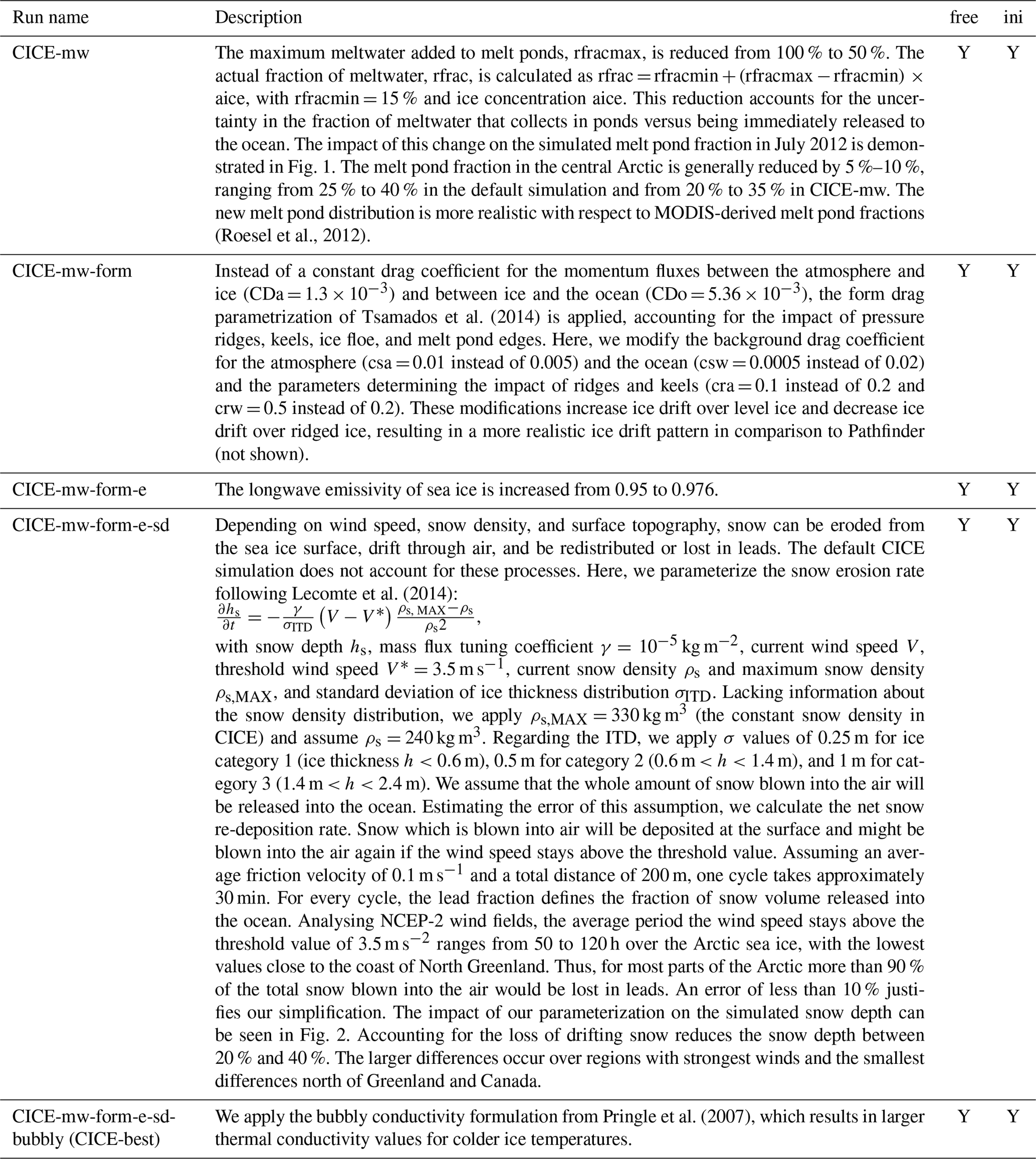
Table 1Simulations with perturbed physical parameterizations improving sea ice thickness. Note that all model changes are cumulative. “Free” indicates multi-year simulations from 1980 to 2017; “ini” indicates the seven 1-year-long simulations starting in mid-November with CS2 sea ice thickness (2010/11 to 2016/17).
3.3 Simulations with perturbed physical parameterizations and sensitivity simulations
3.3.1 Improving sea ice thickness
Comparing the CICE simulation with CS2 reveals that CICE-default underestimates the mean monthly sea ice thickness by about 0.8 m (see Fig. 1a and discussion in Sect. 4). This motivates experiments with perturbed physical parameterizations aiming to increase ice thickness. All additional simulations are listed and described in Table 1. They have been performed as multi-year simulations (1980 to 2017, CICE-free) and seven 1-year-long simulations initialized with CS2 ice thickness (CICE-ini).
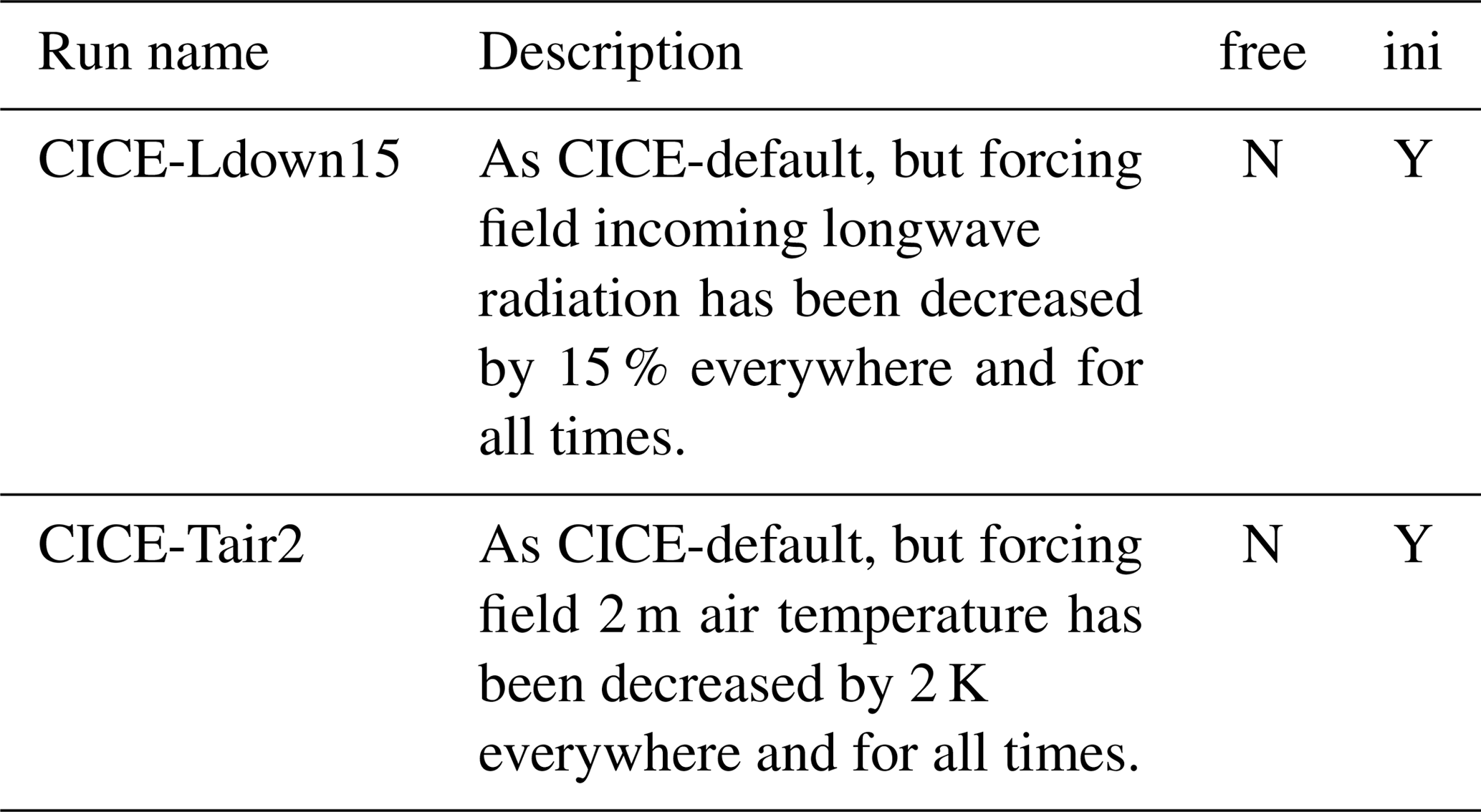
Table 2Sensitivity simulations exploring the impact of uncertainty in atmospheric forcing data. “Free” indicates multi-year simulations from 1980 to 2017; “ini” indicates seven 1-year-long simulations starting in mid-November with CS2 sea ice thickness (2010/11 to 2016/17).
3.3.2 Uncertainty in atmospheric forcing data
We perform two sensitivity experiments to explore the impact of uncertainty in atmospheric forcing on simulated sea ice conditions: a decrease of incoming longwave radiation by 15 % and a decrease of 2 m air temperature by 2 K during the whole simulation. For both experiments, seven 1-year-long simulations are performed which are initialized with CS2 ice thickness (CICE-ini) in mid-November. The set-up of the reference run has been applied (CICE-default). See Table 2 for details.
Table 3Sensitivity simulations exploring the impact of initial and forcing conditions. “Free” indicates multi-year simulations from 1980 to 2017; “ini” indicates seven 1-year-long simulations starting in mid-November with CS2 sea ice thickness (2010/11 to 2016/17). The model configuration for all simulations is CICE-best.

3.3.3 Impact of initial conditions and atmospheric forcing data
We perform additional sensitivity experiments to explore the impact of initial and forcing conditions. Therefore, we conduct simulations with climatological initial and forcing conditions. For each experiment, seven 1-year-long simulations are performed that are initialized with CS2 ice thickness (CICE-ini) in mid-November. The set-up of the most realistic configuration has been applied (CICE-best). See Table 3 for details and Sect. 4.4 for deriving our most realistic configuration.
4.1 Defining region for comparing model sea ice thickness with CryoSat-2 data
Several factors lead to errors in ice thickness retrieval from CS2, in particular the assumption of a climatological snow depth. The resulting ice thickness error is about 5 times larger than the error in snow depth; e.g. an underestimation in snow depth of 0.1 m leads to an underestimation in ice thickness of 0.5 m for a typical ice freeboard of 0.2 m (Tilling et al., 2015).
To enable a meaningful comparison of simulated sea ice thickness between CICE and CS2, we have to reduce the impact of errors. While for individual years and regions the W99 snow load can differ from reality by more than 0.1 m (Warren et al., 1999), the average snow conditions are accurately represented, at least over multi-year ice (e.g. Haas et al., 2017). Over first-year ice, snow depth is overestimated (Kurtz and Farrell, 2011; Webster et al., 2014); hence CS2 retrievals halve W99 snow depth (Sect. 1). We will compare multi-year monthly means over the CS2 period 2010 to 2017. Further, we compare spatial averages of ice thickness to reduce the impact of random errors. A recent study by Nandan et al. (2017) showed that a vertical shift in the scattering horizon due to snow salinity could lead to an overestimation of CS2 ice thickness over first-year ice. Our region combines multi-year ice and first-year sea ice with a ratio of 65:35.
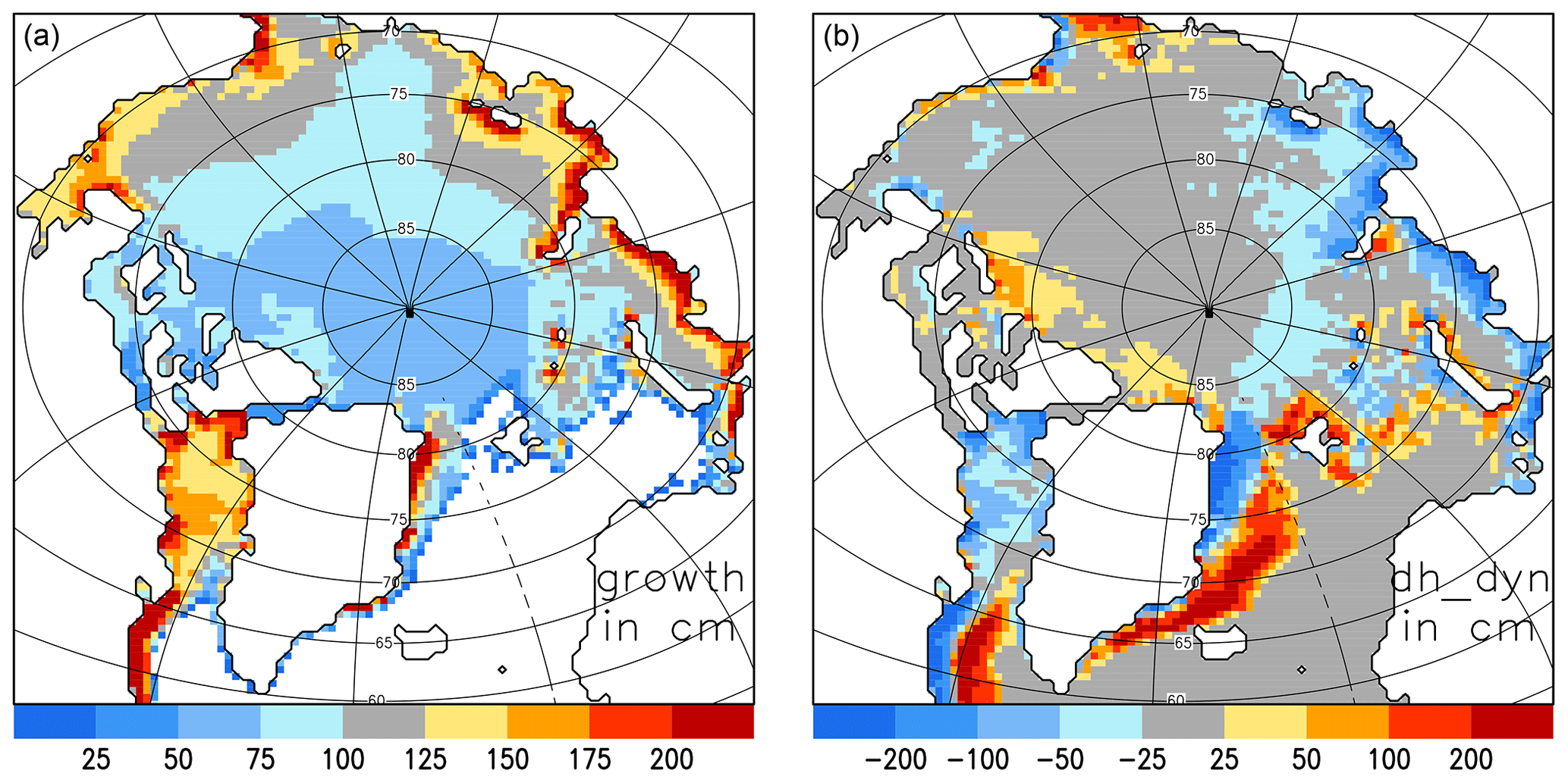
Figure 2Mean simulated sea ice thickness change from November to April (2010–2016) in CICE-default: (a) sea ice growth in centimetres and (b) sea ice thickness change by dynamical processes dh_dyn in centimetres (advection, convergence, and ridging).
We select a region over which to compare model simulations with CS2 data, for which CS2 data exist for all winter periods with at least 100 single observations per month and grid cell, and a minimum mean ice thickness of 0.5 m. Focusing on winter ice growth, we limit the region even further to grid cells in which ice growth is dominating over the impact of dynamics on sea ice thickness change. The mean simulated ice growth from November to April (2010 to 2016; see Fig. 2a) varies between 0.6 and 1.0 m in the central Arctic and can reach values of more than 2 m in the polynya regions along the Siberian coast (Dmitrenko et al., 2009; Bauer et al., 2013). Ice thickness is also modified by dynamical processes such as advection, convergence, and ridging. While the total impact is below ±0.25 m in the central Arctic, more than 2 m of ice is exported on average from some coastal regions and transported to the Fram Strait (see Fig. 2b). For our region of interest, we only select grid cells in which the impact of dynamics on sea ice thickness change during winter is less than 0.25 m in magnitude. The resulting comparison region restricted by CS2 observations and dynamical sea ice change is shown in Fig. 3. We use this region for the rest of the paper.

Figure 3Region for comparing CICE and CS2 sea ice thickness where impact of winter growth on thickness change dominates other factors and where CS2 data are most accurate (see Sect. 4.1 for more details).
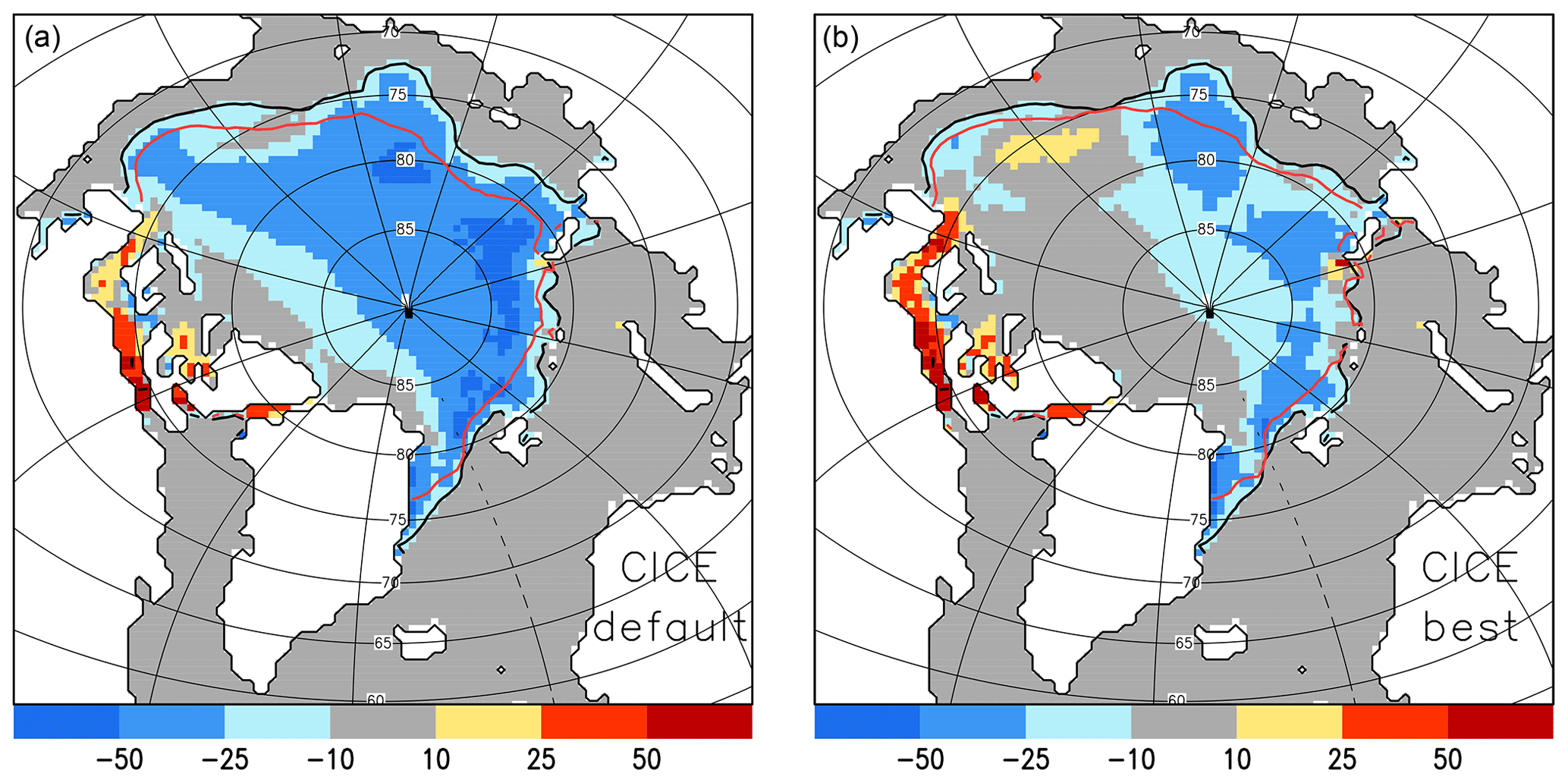
Figure 4Difference in mean September sea ice concentration (2005–2014) in % between the CICE simulation and SSM/I Bootstrap data. Negative values mean lower ice concentration in CICE. The black line indicates mean SSM/I and the red line the mean CICE sea ice extent: (a) CICE-default and (b) CICE-best.
4.2 Comparison of default CICE simulation with CryoSat-2 data
The mean annual cycle of ice thickness over our region of interest is compared in Fig. 1 with CS2. CICE-free-default underestimates the mean monthly sea ice thickness by about 0.8 m. It is noteworthy that this simulation is generally realistic in comparison to SSM/I (Special Sensor Microwave/Imager) sea ice extent (see Fig. 4) and represents the inter-annual variability of, e.g. the September ice extent. The magnitude of the ice thickness difference of 0.8 m cannot be explained by the uncertainty of the CS2 ice thickness alone (Tilling et al., 2016; Stroeve et al., 2018) and so indicates a model error.
CS2 ITD can be applied to initialize a CICE simulation with the observed ice thickness and CS2 data enable us to trace the ice thickness continuously through the whole winter until April. We apply the mean November CS2 ITD to initialize the CICE simulations in mid-November for the years from 2010 to 2016. Starting in mid-November, the mean simulated April ice thickness from CICE-ini-default is about 0.25 m too thin (Fig. 1b). This indicates that the winter ice growth is underestimated in the model. To explore the reasons for the underestimation, we will first examine the impact of atmospheric forcing data (Sect. 4.3) and then the impact of the physical processes involved and how they are represented in CICE (Sect. 4.4).
4.3 Impact of uncertainty in atmospheric forcing data
CICE ice growth in the central Arctic mainly depends on atmospheric forcing (in particular incoming longwave radiation and air temperature), the parameterization of the turbulent atmospheric heat fluxes (heat transfer coefficients), and the conductive heat fluxes within the ice and snow layers. While the impact of the turbulent ocean heat flux under the ice can be large in the marginal ice zone, the ocean temperature is generally close to the freezing temperature in the central Arctic during winter.
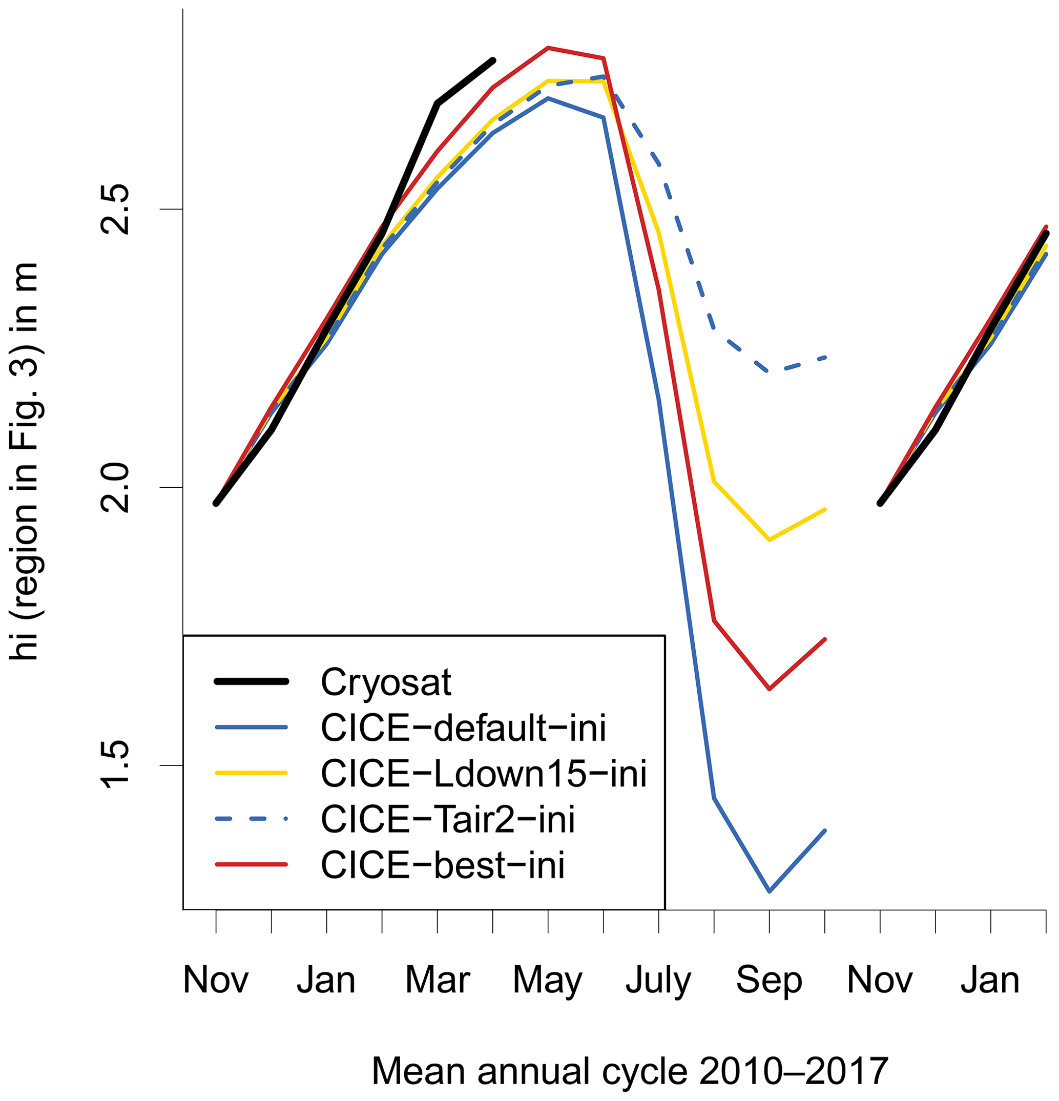
Figure 5Impact of uncertainty in atmospheric forcing on simulated mean effective sea ice thickness over the region shown in Fig. 3 and averaged over winter periods 2010/11 to 2016/17. CICE-ini simulations: default, default with increase of incoming longwave radiation of 15 W m−2, default with increase of 2 m air temperature of 2 K (everywhere and anytime), and best. Model results are compared with mean sea ice thickness from CS2 CPOM.
To explore to what extent the underestimation of ice thickness can be attributed to errors in the surface energy balance associated with atmospheric forcing data, we performed two sensitivity studies in which we decreased (1) the incoming longwave radiation by 15 W m−2 (CICE-Ldown15-ini) and (2) the 2 m air temperature (CICE-Tair2-ini) during the whole simulation period and for every location (see Table 2). We have chosen these values as estimates for potential total systematic atmospheric errors (e.g. Chaudhuri et al., 2014). The impact of these atmospheric perturbations on ice growth is small (see Fig. 5) and the gap between CS2 ice thickness and CICE-default ice thickness can only be reduced marginally. The reduced longwave radiation and air temperature lead to a reduction of ice surface temperature in the range of 2 to 3 K and only increase ice growth by about 5 % each. This is due to the fact that surface temperatures are around −30 ∘C during winter and the conductivity of the snow layer is low. Winter ice growth is not strongly affected by errors in atmospheric conditions. This is fundamentally different during the melting season. Figure 5 reveals that the sea ice would be 0.9 m thicker in September due to the reduction of incoming longwave radiation and 1.4 m thicker due to the decrease of 2 m air temperature, starting with the same initial conditions in the November of the previous year. These sensitivity studies reveal that the underestimation of winter ice growth cannot be explained by errors in the surface energy balance associated with atmospheric forcing data.
4.4 Improving CICE simulation by varying model physics
In the sea ice model, local ice thickness changes are calculated by thermodynamic processes (ice growth and melt) and dynamic processes (advection and ridging). The thermodynamic change depends on the energy balance at the interfaces between the atmosphere, snow, ice, and the ocean derived from the shortwave and longwave radiation fluxes, the turbulent heat fluxes, and the conductive heat flux through the ice and snow. Addressing the individual contributions systematically, we alter model physics within their range of uncertainty with the aim to increase sea ice thickness. Our model changes are presented in a cumulative way.
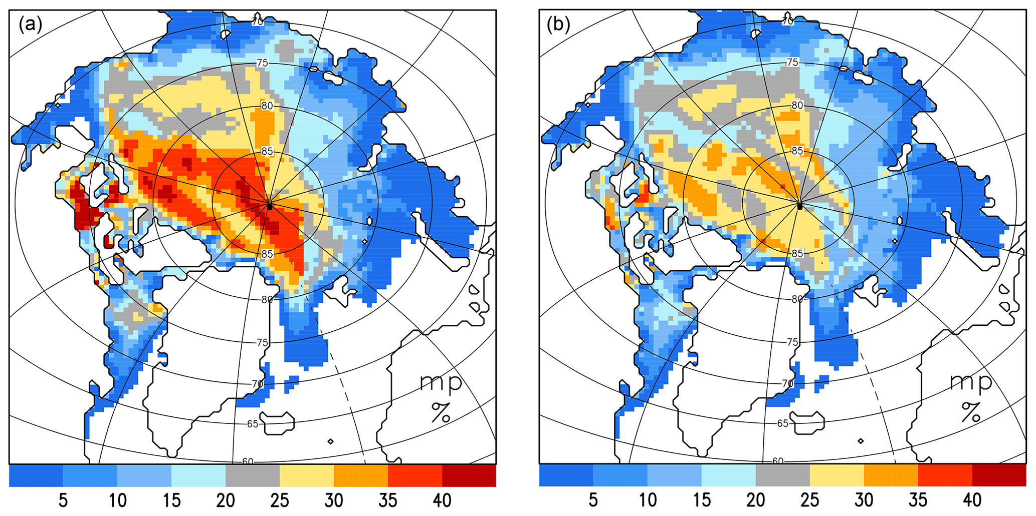
Figure 6Impact of reduced retained meltwater fraction on simulated melt pond area fraction in July 2012: (a) CICE-default and (b) CICE-mw.
The shortwave radiation budget strongly depends on the surface albedo parameterization. Here, we indirectly increase the total ice surface albedo (accounting for snow-covered ice and pond-covered ice, as well as bare ice) by releasing more meltwater into the ocean, and hence reducing the formation of ponded (darker) water over the surface of the ice (CICE-mw; see Table 1). While there are several possibilities to increase albedo values, we selected the release of meltwater because of its impact on the albedo feedback mechanism and the poor knowledge about realistic assumptions. The impact on the simulated melt pond fraction can be seen in Fig. 6 for July 2012. Comparing our simulated melt pond fraction with satellite products (not shown) shows that the mean July pond fraction of CICE-mw (25 %) is closer to the mean values based on MERIS (Istomina et al., 2015) and MODIS data (Roesel et al., 2012) (24 % for both) than the mean pond fraction of CICE-default (28 %). Furthermore, the rms error with respect to MERIS is reduced from 16 % (CICE-default) to 14 % (CICE-mw), justifying our increased release of meltwater. Figure 1a shows that the thickness error is marginally reduced by CICE-mw from about 0.8 to 0.70–0.75 m. As expected there is no impact during winter for the initialized simulation, but the summer ice is 0.2 m thicker (Fig. 1b).
In the next experiment, we address the sea ice advection and the turbulent heat fluxes. We apply the form drag parameterization of Tsamados et al. (2014) in addition to the release of more meltwater (CICE-mw-form). Ice thickness increased slightly with respect to CICE-mw due to a reduced ice drift speed, resulting in a weaker ocean–ice heat flux and less ice export. In addition, increasing the emissivity of snow and ice from 0.95 to 0.976 (CICE-mw-form-e) affects the longwave radiation budget. The increase reduces summer melt by a few centimetres, but no impact during winter is visible.
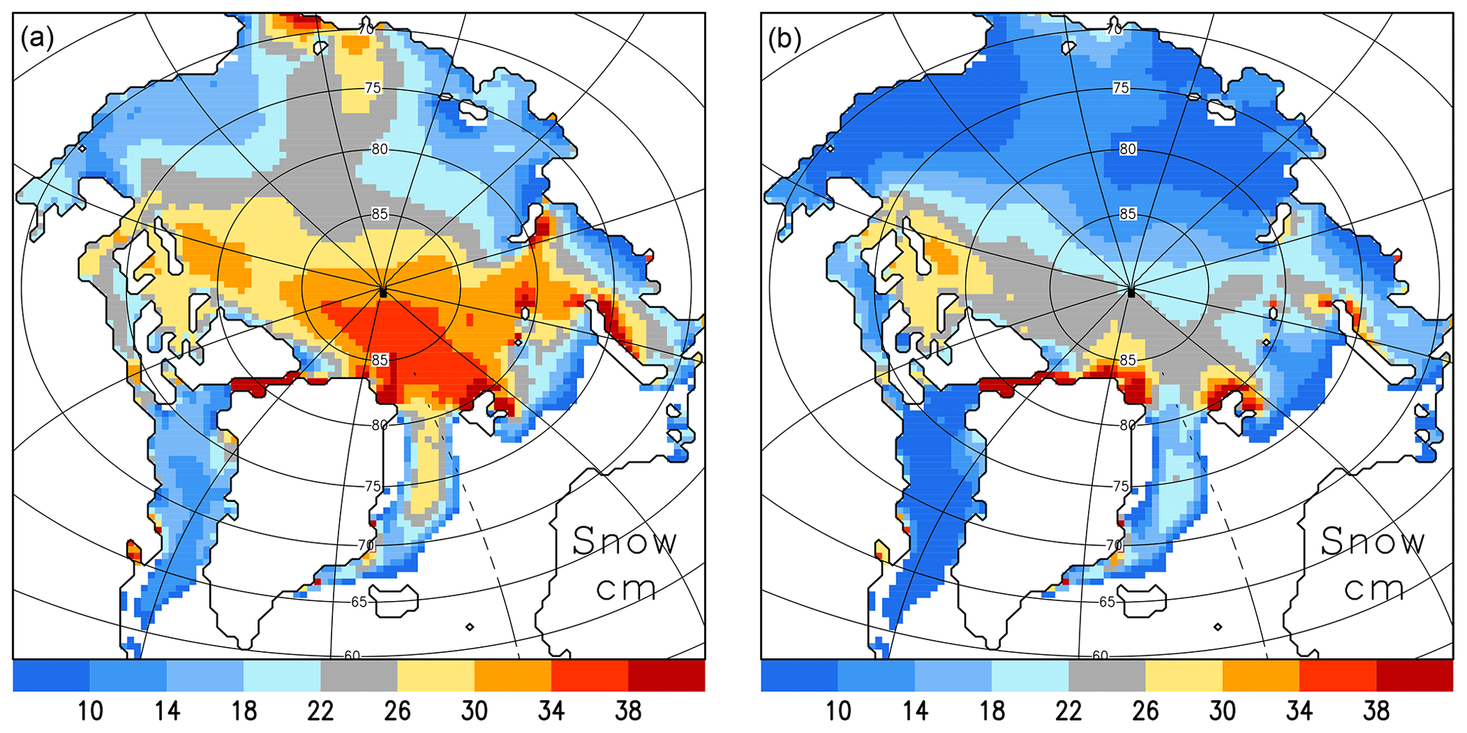
Figure 7Impact of snow erosion on simulated mean April snow depth (2010 to 2017): (a) CICE-default and (b) CICE-mw-from-e-sd.
Due to its low conductivity, snow depth controls the conductive heat flux. Here, we implement a snow drift scheme based on Lecomte et al. (2014) which reduces the snow depth by 20 % to 40 % (CICE-mw-form-e-sd; see Fig. 7) and has the biggest impact on sea ice thickness from all individual changes. With respect to CICE-default, the thickness error has been reduced from 0.8 to 0.25 m (see CICE-mw-form-e-sd-free in Fig. 1a). The reduction of snow depth leads to a strong increase in ice growth in winter, but also to a moderate increase of summer melt due to an earlier disappearance of snow. This can be seen comparing CICE-mw-form-e-sd-ini with CICE-mw-form-e-ini in Fig. 1b. The reduction of snow leads to an increase of May ice thickness of 0.12 m and to a decrease of September ice thickness of 0.06 m. Applying an increased conductivity coefficient for colder temperature (Pringle et al., 2007; CICE-mw-form-e-sd-bubbly) in addition reduces the error for CICE-free and CICE-ini to less than 0.1 m. This modification increases winter ice growth, but it has no impact during summer.
Table 4Mean area fraction of sea ice per category in % according to CS2 and CICE-best-ini (over the region shown in Fig. 3 and for the period 2010 to 2017).
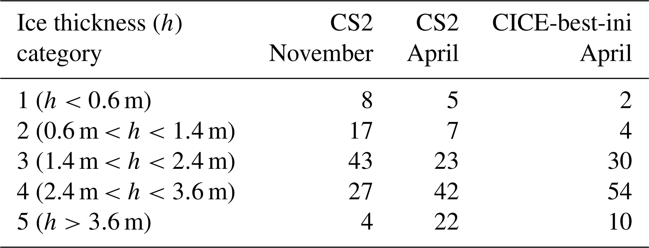
Our selected region for comparing CICE and CS2 ice thickness consists of 35 % first-year and 65 % multi-year ice. The area fraction for each of the five ice thickness categories is shown in Table 4. In November, 25 % of the region is covered by ice which is thinner than 1.4 m and 4 % by ice which is thicker than 3.6 m according to CS2. In April the thin ice fraction reduced to 12 % and thick ice fraction increased to 22 %. While the mean ice thickness between CICE-best-ini and CS2 is very similar, the thickness distribution is a bit narrower in CICE in April: 6 % of area thinner than 1.4 m and 10 % thicker than 3.6 m.
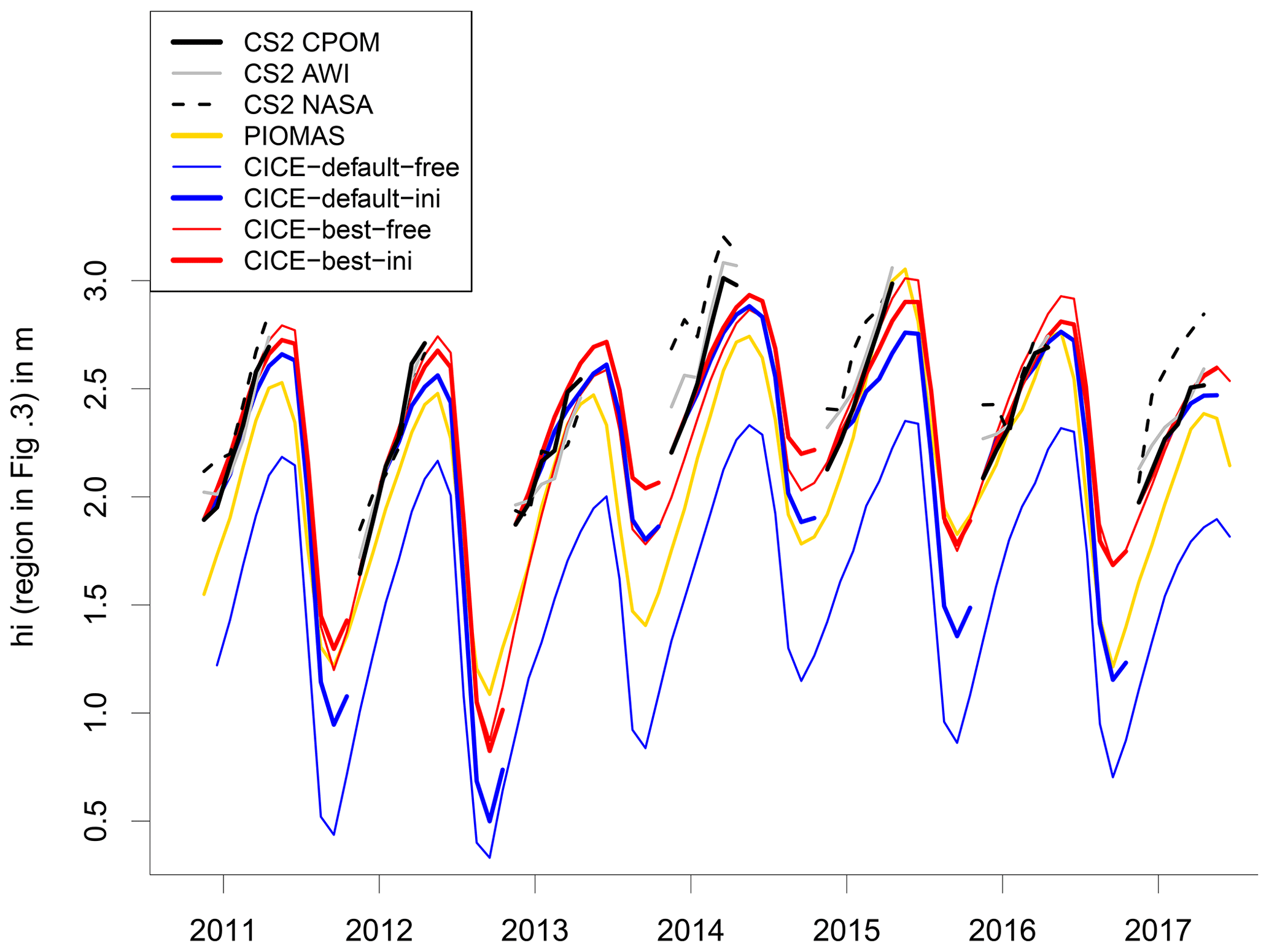
Figure 8Mean effective sea ice thickness over the region shown in Fig. 3. Verification of CICE-free default and best (thin lines) and CICE-ini default and best (thick lines) with CS2 CPOM, AWI, NASA, and PIOMAS.
So far, we have compared the mean annual cycle of sea ice thickness over the period from 2010 to 2017. Figure 8 compares times series of the individual years from free and initialized CICE simulations with three different CS2 products provided by CPOM, AWI and NASA. For all years, CICE-best-free is much closer to CS2 than CICE-default-free. It is striking that differences between CICE-best-free and CICE-best-ini are small. This is a remarkable result from a modelling point of view because it means that CICE-best is so realistic that the assimilation of sea ice thickness would not result in substantial changes. This agreement increases the confidence in our new model set-up.
Naturally, differences between CS2 and CICE-best remain. In November 2012, simulated ice is about 0.5 m thinner than in CS2. During winter 2013/14 the CS2-CPOM ice growth is stronger than in CICE-best-ini with large differences between the three CS2 products. These differences can be caused either by model errors or by errors estimating sea ice thickness from CS2. As discussed in Sect. 4.1, using a climatological snow depth limits the applicability to derive inter-annual variability from CS2 ice thickness. For comparison, mean sea ice thickness from PIOMAS (Zhang and Rothrock, 2003) is added in Fig. 8. Although no sea ice thickness observations are assimilated, PIOMAS is widely applied for the verification of climate models. In spite of some differences between PIOMAS, CS2, and CICE-best in the sea ice thickness evolution, the general statement that CICE-best is more realistic than CICE-default is confirmed by PIOMAS.
As the summer sea ice extent is quite realistic in CICE-default (Sect. 4.2), we investigate the impact of the strong ice thickness increase in CICE-best on sea ice concentration and extent. Figure 4a reveals that the mean September sea ice extent over the period 2005–2014 is slightly underestimated in CICE-default with respect to SSM/I Bootstrap (Comiso, 1999). The impact of the strong thickness increase on sea ice extent is small; the ice extent is only marginally larger in CICE-best (Fig. 4b), but nevertheless close to SSM/I Bootstrap. In contrast to ice extent, ice concentration is underestimated in CICE-default by 25 % to 50 % in large parts of the ice-covered Arctic Ocean. While apart from the ice edge, ice concentration is generally between 80 % and 100 % according to SSM/I Bootstrap, CICE-default frequently shows large areas with values below 50 %. This discrepancy is strongly reduced in CICE-best, with error values below 10 % in the Canadian half and between 10 % and 30 % in the Siberian half of the Arctic (Fig. 4b). It is worth mentioning that nearly all CMIP5 climate models underestimate Arctic summer sea ice concentration in their historical runs with respect to SSM/I Bootstrap (see e.g. Fig. 3 in Notz, 2014). CICE-best does not only improve the sea ice thickness, but also the summer sea ice concentration.
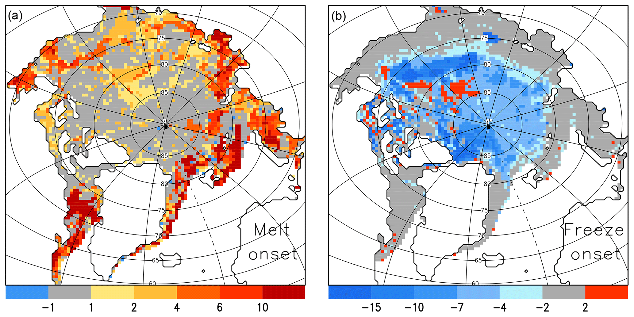
Figure 9Difference in mean melt onset (a) and freeze onset (b) on days between CICE-best and CICE-default (2010–2017). Positive values mean a later onset day in CICE-best.
We demonstrate the impact of our model changes on the timing of mean melt and freeze onset (2005–2014) between CICE-best and CICE-default in Fig. 9. In CICE-best, the melt onset day is later (0–4 days in the central Arctic, up to 10 days in the Fram Strait) and the freeze onset is earlier (4–12 days in most areas), resulting in a shorter melting season. The simulated mean length of the melting season over the Arctic Basin reduces from 107 days (CICE-default) to 100 days (CICE-best). This is an improvement with respect to the observed value of 94 days. The observed number of 94 days is based on a mean value of 88 days for the period 1979 to 2012 and accounting for the trend of 3.7 days decades−1 (Stroeve et al., 2014). The impact of the model changes is remarkable given that we apply the same 2 m air temperature data (NCEP-2) as atmospheric forcing. Our examples indicate that the chosen model physics may be important for many climate-related questions and how climate models predict future changes of summer melting season and sea ice decline.

Figure 10Impact of climatological initial conditions (climini), climatological forcing (climforcing), and climatological forcing during winter only (November to April, climforcing-winter). All CICE simulations from CICE-ini best. Mean effective sea ice thickness over the region is shown in Fig. 3. CS2 as in Fig. 7. The climatology is calculated over the period 2011 to 2017 for air temperature, humidity, downward longwave and shortwave radiation, rainfall, and snowfall. The real wind forcing is applied in all simulations.
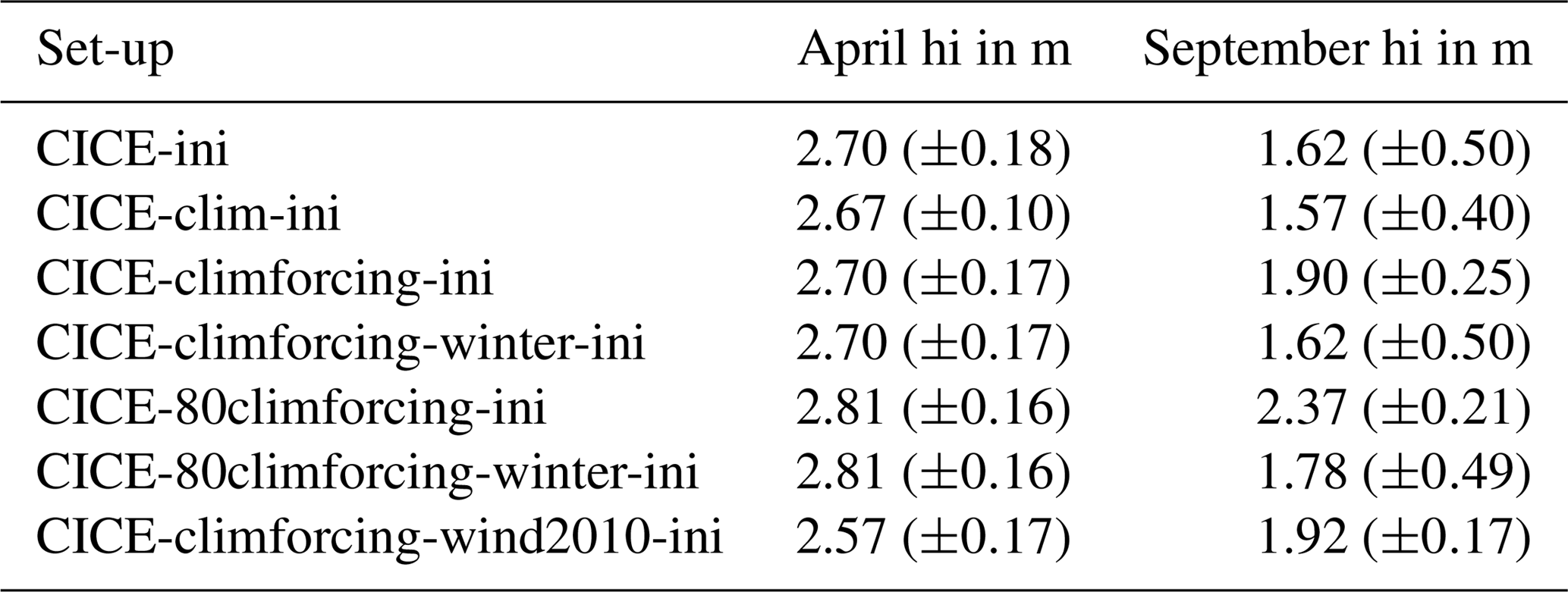
Table 5Impact of initial November sea ice conditions and atmospheric forcing on the mean sea ice thickness (hi) of subsequent April and September over the region shown in Fig. 3 from 2011 to 2017. See Sect. 3.3 for explanation of CICE simulations. Inter-annual variability is given in parentheses.
4.5 Impact of initial conditions and atmospheric forcing
How strongly do the CICE simulations depend on sea ice initial conditions? Using the mean CS2 November sea ice thickness from 2010 to 2016 (CICE-climini; Table 3) instead of the annual values leads to positive or negative thickness anomalies which remain throughout the year, becoming only slightly weaker during winter (Fig. 10). The inter-annual variability of the simulated April ice thickness is reduced by 44 % (from 0.18 to 0.10 m, Table 5) and the September ice thickness by 20 % (from 0.5 to 0.4 m).
Applying a mean atmospheric forcing for each year (CICE-climforcing-ini) hardly affects the ice thickness during winter (with the exception of winter 2016/17), but it leads to strong anomalies during summer (Fig. 10). The mean September sea ice thickness is increased by 0.28 m and the inter-annual variability reduced from 0.5 to 0.25 m (Table 5). Applying the mean atmospheric forcing during winter only and the individual atmospheric forcing from May onwards (CICE-climforcing-winter-ini), sea ice thickness during summer is nearly unchanged with respect to CICE-ini. While the atmospheric conditions during summer are decisive for summer ice melt and September sea ice thickness, the atmospheric winter conditions seem not to matter at all.

The atmospheric conditions for the last eight winters were all relatively warm with respect to the 1980 to 2010 climate. Is it possible that the small variability of these winter periods could cause the weak impact on sea ice thickness? To exclude this possibility, we perform additional sensitivity experiments in which we apply colder atmospheric conditions from the 1980s (CICE-80climforcing-ini). Figure 11 and Table 3 reveal that the impact during winter is nevertheless small (mean thickness increase of 0.11 m), but huge in summer (+0.8 m). Interestingly, the impact of using the wind forcing from an anomalous year (2009/10, stronger transpolar-drift), CICE-climforcing-wind20100ini, is stronger on April ice thickness (−0.13 m) than from the cold atmospheric conditions. This confirms the important role of sea ice dynamics and export through the Fram Strait in controlling the sea ice volume variability (Ricker et al., 2018).
These sensitivity experiments demonstrate that the atmospheric winter conditions have a very small impact on winter ice growth and thus on April ice thickness. September ice thickness depends strongly on atmospheric conditions from May to September.
We determined an optimal region for comparing sea ice thickness between simulations with the sea ice model CICE and CS2 data by taking into account the strengths and weaknesses of both approaches. Since simulating dynamic processes can result in large model errors and can be proportionally less accurate, we exclude locations where sea ice dynamics (sea ice advection and ridging) make a strong contribution to the modification of sea ice thickness. We further exclude locations where the number of CS2 observations is limited and the sea ice is thin during winter (<0.5 m). The resulting region includes most of the central Arctic, but not the area of the thickest ice north of Canada or any of the shelf seas (see Fig. 3).
Comparing the multi-year means reveals that CICE-default underestimates ice thickness over our comparison region by about 0.8 m (see Fig. 1a). This discrepancy would not have been identified by comparing total Arctic ice volume. Due to overestimating ice thickness in the Canadian sector, Arctic ice volume from CICE-default is only slightly lower than estimates based on CS2 or PIOMAS. Deriving the sub-grid-scale ice thickness distribution (ITD) from CS2 allows us to initialize CICE simulations with the identical ice thickness in November. Applying default settings CICE-ini underestimates mean ice thickness in the following April by 0.25 m (see Fig. 1b). This indicates that the winter ice growth is too weak in the model. What is the reason for the underestimation of ice growth? Our sensitivity experiments give evidence that uncertainty in atmospheric forcing cannot be the main reason. The impact of errors in air temperature and incoming longwave radiation on sea ice growth is rather small in winter (see Fig. 5). The turbulent ocean–ice heat flux is generally small in winter in the central Arctic; thus, errors deriving from the turbulent ocean–ice heat flux cannot be responsible either. The ice–atmosphere heat fluxes depend on atmospheric forcing and the transfer coefficients. Varying the transfer coefficients does not result in major changes of sea ice growth. Initial conditions in autumn are important, but our initialized CICE simulations show that April ice thickness is still underestimated even when starting with the “correct” November ice thickness. Thus, by a process of exclusion, we conclude that sea ice physics related to the conductive flux must be responsible.
The strongest contribution to the simulation of winter ice growth comes from implementing a snow drift scheme based on Lecomte et al. (2014). Although our implementation is simple and further work to improve the parameterization is required, it demonstrates the importance of including additional snow processes in sea ice models for climate applications (Vionnet et al., 2012; Nandan et al., 2017; Liston et al., 2018). Such model development can also benefit recent Arctic-wide snow products that rely on satellite observations (Maaß et al., 2013; Guerreiro et al., 2016; Lawrence et al., 2018) or reanalysis precipitation fields that rely on drifting sea ice (Kwok and Cunningham, 2008).
Our sensitivity experiments modifying initial and atmospheric forcing data reveal that ice thickness anomalies in November decay over winter but are still present in the following April (see Fig. 10). Comparing inter-annual variability of April ice thickness between CICE-ini and CICE-climini (Table 5) shows that half of the variability comes from the initial conditions. Atmospheric conditions during spring and summer are decisive for summer sea ice conditions, but atmospheric winter conditions have little impact on sea ice growth. Using “cold” forcing from the 1980s instead of the more recent winters leads to an increase in September sea ice thickness of 0.8 m, but only to an increase in April ice thickness of 0.11 m (see Fig. 11 and Table 5). This reflects the importance of feedback processes. During winter, the negative conductive feedback process (less ice, more growth) is dominating, while during summer the positive albedo feedback process determines sea ice changes. The impact of the negative winter feedback has been discussed in Stroeve et al. (2018). In their study, a potential weakening of the feedback during the last years has been raised as a question. Here, we answer this question, demonstrating that warm winters are not important for observed sea ice thinning in recent decades, at least in the central Arctic. The situation can be different in the marginal winter sea ice zone, where a warm winter can increase mixed-layer ocean temperature and delay ice growth. Our findings are in agreement with observations of recent years: in spite of the three warmest Arctic-wide winter air temperatures during 2014/15, 2015/16, and 2016/17 on record (Stroeve et al., 2018), the September Arctic sea ice extent in 2015 (4.7 million km2), 2016 (4.7 million km2), and 2017 (4.9 million km2) was larger than in 2012 (3.6 million km2); these numbers are based on SSM/I NASA-Team algorithm (Cavalieri et al., 1996, updated 2017). We conclude that the fate of Arctic summer sea ice depends largely on atmospheric spring and summer conditions, in particular May and June, when the melting season starts and melt ponds form, preconditioning the strength of the positive albedo feedback mechanism (Schröder et al., 2014).
Our optimal model configuration CICE-best does not only improve the simulation of mean sea ice thickness over the central Arctic with respect to CS2, but also improves summer sea ice concentration (in comparison to SSM/I Bootstrap), the length of the melt season (in comparison to Stroeve et al., 2014), and the melt pond fraction (in comparison to MODIS and MERIS). Recent studies have demonstrated improvements for sea ice predictions up to 6 months, initializing forecast models with CS-2 data (Allard et al., 2018; Blockley and Peterson, 2018). Here, we show that our improvements to the sea ice model CICE are so fundamental and consistent that any differences between CICE simulations initialized by CS2 ice thickness and those which do not utilize them are minimized. It is the first time CS2 sea ice thickness data have been applied successfully to improve sea ice model physics.
Model results from all CICE simulations listed in Tables 1–3 are available here: http://dx.doi.org/10.17864/1947.187 (Schröder, 2018). The AWI data are available from https://www.meereisportal.de/ (last access: December 2017), the CPOM data are available from http://www.cpom.ucl.ac.uk/csopr/seaice.html (last access: December 2017), NASA data are available from: https://nsidc.org/data/RDEFT4/ (Kurtz and Harbeck, 2017). NCEP2 data obtained from NOAA Earth System Research Laboratory (http://www.esrl.noaa.gov/psd/data/gridded/data.ncep.reanalysis2.gaussian.html, last access: December 2017).
AR, RT, and MT prepared the Cyrosat-2 data. DS performed the CICE simulations. All authors contributed to the composition of the paper and the discussion of the results.
The authors declare that they have no conflict of interest.
This work was done under the ACSIS and UKESM program funded by the UK
Natural Environment Research Council. The authors would like to thank the
Isaac Newton Institute for Mathematical Sciences for support and hospitality
during the programme Mathematics of Sea Ice Phenomena, when work on this paper
was undertaken. This work was supported by EPSRC grant number
EP/K032208/1. Michel Tsamados acknowledges the support from the
Arctic + European Space Agency snow project ESA/AO/1-8377/15/I-NB NB –
STSE – Arctic+.
Edited by: John Yackel
Reviewed by: two anonymous referees
Allard, R. A., Farrell, S. L., Hebert, D. A., Johnston, W. F., Li, L., Kurtz, N. T., Phelps, M. W., Posey, P. G., Tilling, R., Ridout, A., and Wallcraft, A. J.: Utilizing CryoSat-2 sea ice thickness to initialize a coupled ice-ocean modeling system, Adv. Space Res., 62, 1265–1280, https://doi.org/10.1016/j.asr.2017.12.030, 2018.
Bauer, M., Schröder, D., Heinemann, G., Willmes, S., and Ebner, L.: Quantifying polynya ice production in the Laptev Sea with the COSMO model, Polar Res., 32, 20922, https://doi.org/10.3402/polar.v32i0.20922, 2013.
Bitz, C. and Lipscomb, W.: An energy-conserving thermodynamic model of sea ice, J. Geophys. Res., 104, 15669–15677, https://doi.org/10.1029/1999JC900100, 1999.
Blockley, E. W. and Peterson, K. A.: Improving Met Office seasonal predictions of Arctic sea ice using assimilation of CryoSat-2 thickness, The Cryosphere, 12, 3419–3438, https://doi.org/10.5194/tc-12-3419-2018, 2018.
Briegleb, B. P. and Light, B.: A delta-Eddington multiple scattering parameterization for solar radiation in the sea ice component of the Com- munity Climate System Model, Tech. Note 472, Natl. Cent. for Atmos. Res., Boulder, CO, 2007.
Cavalieri, D., Parkinson, C., Gloersen, P., and Zwally, H. J.: Sea Ice Concentrations from Nimbus-7 SMMR and DMSP SSM/I-SSMIS Passive Microwave Data, Boulder, Colorado USA, NASA DAAC at the National Snow and Ice Data Center, 1996 (updated 2017).
Chaudhuri, A. H., Ponte, R. M., and Nguyen, A. T.: A Comparison of Atmospheric Reanalysis Products for the Arctic Ocean and Implications for Uncertainties in Air-Sea Fluxes, J. Climate, 27, 5411–5421, https://doi.org/10.1175/JCLI-D-13-00424.1, 2014.
Comiso, J.: Bootstrap Sea Ice Concentrations From NIMBUS-7 SMMR and DMSP SSM/I, available at: http://nsidc.org/data/nsidc-0079.html (last access: December 2017), Natl. Snow and Ice Data Cent., Boulder, CO, 1999 (updated 2017).
Dmitrenko, I. A., Kirillov, S. A., Tremblay L. B., Bauch, D., and Willmes, S.: Sea-ice production over the Laptev Sea Shelf inferred from historical summer-to-winter hydrographic observations of 1960s to 1990s, Geophys. Res. Lett. 36, L13605, https://doi.org/10.1029/2009GL038775, 2009.
Ferry, N., Masina, S., Storto, A., Haines, K., Valdivieso, M., Barnier, B., and Molines, J.-M.: Product User Manual GLOBAL-REANALYSISPHYS-001-004-a and b, MyOcean, 2011.
Flocco, D., Feltham, D. L., and Turner, A. K.: Incorporation of a physically based melt pond scheme into the sea ice component of a climate model, J. Geophys. Res., 115, C08012, https://doi.org/10.1029/2009JC005568, 2010.
Flocco, D., Schröder, D., Feltham, D. L., and Hunke, E. C.: Impact of melt ponds on Arctic sea ice simulations from 1990 to 2007, J. Geophys. Res., 117, C09032, https://doi.org/10.1029/2012JC008195, 2012.
Giles, K. A., Laxon, S. W., Wingham, D. J., Wallis, D. W., Krabill, W. B., Leuschen, C. J., McAdoo, D., Manizade, S. S., and Raney, R. K.: Combined airborne laser and radar altimeter measurements over the Fram Strait in May 2002, Remote Sens. Environ., 111, 182–194, https://doi.org/10.1016/j.rse.2007.02.037, 2007.
Giles, K. A., Laxon, S. W., and Ridout, A. L.: Circumpolar thinning of Arctic sea ice following the 2007 record ice extent minimum, Geophys. Res. Lett., 35, L22502, https://doi.org/10.1029/2008GL035710, 2008.
Guerreiro, K., Fleury, S., Zakharova, E., Rémy, F., and Kouraev, A.: Potential for estimation of snow depth on Arctic sea ice from CryoSat-2 and SARAL/AltiKa missions, Remote Sens. Environ., 186, 339–349, 2016.
Haas, C., Beckers, J., King, J., Silis, A., Stroeve, J., Wilkinson, J., Notenboom, B., Schweiger, A., and Hendricks, S.: Ice and snow thickness variability and change in the high Arctic Ocean observed by in situ measurements, Geophys. Res. Lett., 44, 10462–10469, https://doi.org/10.1002/2017GL075434, 2017.
Hendricks, S., Ricker, R., and Helm, V.: User Guide – AWI CryoSat-2 Sea Ice Thickness Data Product (v1.2), hdl:10013/epic.48201, 2016.
Heorton, H., Feltham, D. L., and Tsamados, M.: Stress and deformation characteristics of sea ice in a high resolution, anisotropic sea ice model, Phil. Trans A, 376, 2129, https://doi.org/10.1098/rsta.2017.0349, 2018.
Hunke, E. C., Lipscomb, W. H., Turner, A. K., Jeffery, N., and Elliott, S.: CICE: the Los Alamos Sea Ice Model Documentation and Software User's Manual Version 5.1, 2015.
Istomina, L., Heygster, G., Huntemann, M., Schwarz, P., Birnbaum, G., Scharien, R., Polashenski, C., Perovich, D., Zege, E., Malinka, A., Prikhach, A., and Katsev, I.: Melt pond fraction and spectral sea ice albedo retrieval from MERIS data – Part 1: Validation against in situ, aerial, and ship cruise data, The Cryosphere, 9, 1551–1566, https://doi.org/10.5194/tc-9-1551-2015, 2015.
Kanamitsu, M., Ebisuzaki, W., Woollen, J., Yang, S.-K., Hnilo, J. J., Fiorino, M., and Potter, G. L.: NCEP-DOE AMIP-II Reanalysis (R-2), B. Am. Meteorol. Soc., 83, 1631–1643, 2017.
Kurtz, N. T. and Farrell, S. L.: Large-scale surveys of snow depth on Arctic sea ice from Operation IceBridge, Geophys. Res. Lett., 38, L20505, https://doi.org/10.1029/2011GL049216, 2011.
Kurtz, N. T., Farrell, S. L., Studinger, M., Galin, N., Harbeck, J. P., Lindsay, R., Onana, V. D., Panzer, B., and Sonntag, J. G.: Sea ice thickness, freeboard, and snow depth products from Operation IceBridge airborne data, The Cryosphere, 7, 1035–1056, https://doi.org/10.5194/tc-7-1035-2013, 2013.
Kurtz, N. T., Galin, N., and Studinger, M.: An improved CryoSat-2 sea ice freeboard retrieval algorithm through the use of waveform fitting, The Cryosphere, 8, 1217–1237, https://doi.org/10.5194/tc-8-1217-2014, 2014.
Kurtz, N. T. and Harbeck, J.: CryoSat-2 Level 4 Sea Ice Elevation, Freeboard, and Thickness, Version 1, Boulder, Colorado USA, NASA National Snow and Ice Data Center Distributed Active Archive Center, 2017.
Kwok, R. and Rothrock, D. A.: Decline in Arctic sea ice thickness from submarine and ICESat records: 1958–2008, Geophys. Res. Lett., 36, L15501, https://doi.org/10.1029/2009GL039035, 2009.
Kwok, R. and Cunningham, G. F.: ICESat over Arctic sea ice: Estimation of snow depth and ice thickness, J. Geophys. Res.-Oceans, 113, https://doi.org/10.1029/2008JC004753, 2008.
Lawrence, I. R., Tsamados, M. C., Stroeve, J. C., Armitage, T. W. K., and Ridout, A. L.: Estimating snow depth over Arctic sea ice from calibrated dual-frequency radar freeboards, The Cryosphere, 12, 3551–3564, https://doi.org/10.5194/tc-12-3551-2018, 2018.
Laxon, S. W., Giles, K. A., Ridout, A. L., Wingham, D. J., Willatt, R., Cullen, R., Kwok, R., Schweiger, A., Zhang, J., Haas, C., Hendricks, S., Krishfield, R., Kurtz, N., Farrell, S., and Davidson, M.: CryoSat-2 estimates of Arctic sea ice thickness and volume, Geophys. Res. Lett., 40, 732–737, https://doi.org/10.1002/grl.50193, 2013.
Lecomte, O., Fichefet, T., Flocco, D., Schröder, D., and Vancoppenolle, M.: Impacts of wind-blown snow redistribution on melt ponds in a coupled ocean – sea ice model, Ocean Model, 87, 67–80, https://doi.org/10.1016/j.ocemod.2014.12.003, 2014.
Lipscomb, W. H. and Hunke, E. C.: Modeling sea ice transport using incremental remapping, Mon. Weather Rev., 132, 1341–1354, 2004.
Liston, G. E., Polashenski, C., Roesel, A., Itkin, P., King, J., Merkouriadi, I., and Haapala, J.: A distributed snow-evolution model for sea-ice applications (SnowModel), J. Geophys. Res.-Ocean, 123, 3786–3810, https://doi.org/10.1002/2017JC013706, 2018.
Maaß, N., Kaleschke, L., Tian-Kunze, X., and Drusch, M.: Snow thickness retrieval over thick Arctic sea ice using SMOS satellite data, The Cryosphere, 7, 1971–1989, https://doi.org/10.5194/tc-7-1971-2013, 2013.
Massonnet, F., Fichefet, T., Goosse, H., Bitz, C. M., Philippon-Berthier, G., Holland, M. M., and Barriat, P.-Y.: Constraining projections of summer Arctic sea ice, The Cryosphere, 6, 1383–1394, https://doi.org/10.5194/tc-6-1383-2012, 2012.
Maykut, G. A. and Untersteiner, N.: Some results from a time-dependent thermodynamic model of sea ice, J. Geophys. Res., 76, 1550–1575, https://doi.org/10.1029/JC076i006p01550, 1971.
Nandan, V., Geldsetzer, T., Yackel, J., Mahmud, M., Scharien, R., Howell, S., King, J., Ricker, R., and Else, B.: Effect of Snow Salinity on CryoSat-2 Arc- tic First-Year Sea Ice Freeboard Measurements, Geophys. Res. Lett., 44, 10419–10426, https://doi.org/10.1002/2017GL074506, 2017.
Notz, D.: Sea-ice extent and its trend provide limited metrics of model performance, The Cryosphere, 8, 229–243, https://doi.org/10.5194/tc-8-229-2014, 2014.
Pringle, D. J., Eicken, H., Trodahl, H. J., and Backstrom, L. G. E.: Thermal conductivity of landfast Antarctic and Arctic sea ice, J. Geophys. Res., 112, C04017, https://doi.org/10.1029/2006JC003641, 2007.
Rae, J. G. L., Hewitt, H. T., Keen, A. B., Ridley, J. K., Edwards, J. M., and Harris, C. M.: A sensitivity study of the sea ice simulation in HadGEM3, Ocean Model, 74, 60–76, https://doi.org/10.1016/j.ocemod.2013.12.003, 2014.
Ricker, R., Hendricks, S., Helm, V., Skourup, H., and Davidson, M.: Sensitivity of CryoSat-2 Arctic sea-ice freeboard and thickness on radar-waveform interpretation, The Cryosphere, 8, 1607–1622, https://doi.org/10.5194/tc-8-1607-2014, 2014.
Ricker, R., Hendricks, S., Kaleschke, L., Tian-Kunze, X., King, J., and Haas, C.: A weekly Arctic sea-ice thickness data record from merged CryoSat-2 and SMOS satellite data, The Cryosphere, 11, 1607–1623, https://doi.org/10.5194/tc-11-1607-2017, 2017.
Ricker, R., Girard-Ardhuin, F., Krumpen, T., and Lique, C.: Satellite-derived sea ice export and its impact on Arctic ice mass balance, The Cryosphere, 12, 3017–3032, https://doi.org/10.5194/tc-12-3017-2018, 2018.
Ridley, J. K., Blockley, E. W., Keen, A. B., Rae, J. G. L., West, A. E., and Schroeder, D.: The sea ice model component of HadGEM3-GC3.1, Geosci. Model Dev., 11, 713–723, https://doi.org/10.5194/gmd-11-713-2018, 2018.
Rösel, A., Kaleschke, L., and Birnbaum, G.: Melt ponds on Arctic sea ice determined from MODIS satellite data using an artificial neural network, The Cryosphere, 6, 431–446, https://doi.org/10.5194/tc-6-431-2012, 2012.
Rothrock, D. A.: The energetics of the plastic deformation of pack ice by ridging, J. Geophys. Res., 80, 4514–4519, https://doi.org/10.1029/JC080i033p04514, 1975.
Rothrock, D. A., Percival, D. B., and Wensnahan, M.: The decline in arctic sea-ice thickness: Separating the spatial, annual, and interannual variability in a quarter century of submarine data, J. Geophys. Res., 113, C05003, https://doi.org/10.1029/2007JC004252, 2008.
Schröder, D., Feltham, D. L., Flocco, D., and Tsamados, M.: September Arctic sea-ice minimum predicted by spring melt-pond fraction, Nat. Clim. Change, 4, 353–357, https://doi.org/10.1038/NCLIMATE2203, 2014.
Schröder, D.: Simulations with the sea ice model CICE documenting the impact of improved sea ice physics, University of Reading, available at: http://dx.doi.org/10.17864/1947.187, 2018.
Shu, Q., Song, Z., and Qiao, F.: Assessment of sea ice simulations in the CMIP5 models, The Cryosphere, 9, 399–409, https://doi.org/10.5194/tc-9-399-2015, 2015.
Stroeve, J. C., Kattsov, V., Barrett, A., Serreze, M., Pavlova, T., Holland, M., and Meier, W. N.: Trends in Arctic sea ice extent from CMIP5, CMIP3 and observations, Geophys. Res. Lett., 39, L16502, https://doi.org/10.1029/2012GL052676, 2012.
Stroeve, J. C., Markus, T., Boisvert, L., Miller, J., and Barrett, A.: Changes in Arctic melt season and implications for sea ice loss, Geophys. Res. Lett., 41, 1216–1225, https://doi.org/10.1002/2013GL058951, 2014.
Stroeve, J. C., Schröder, D., Tsamados, M., and Feltham, D.: Warm winter, thin ice?, The Cryosphere, 12, 1791–1809, https://doi.org/10.5194/tc-12-1791-2018, 2018.
Tilling, R. L., Ridout, A., Shepherd, A., and Wingham, D. J.: Increased arctic sea ice volume after anomalously low melting in 2013, Nat. Geosci., 8, 643–646, 2015.
Tilling, R. L., Ridout, A., and Shepherd, A.: Near-real-time Arctic sea ice thickness and volume from CryoSat-2, The Cryosphere, 10, 2003–2012, https://doi.org/10.5194/tc-10-2003-2016, 2016.
Tilling, R. L., Ridout, A., and Shepherd, A.: Estimating Arctic sea ice thickness and volume using CryoSat-2 radar altimeter data, Adv. Space Res., 62, 1203–1225, https://doi.org/10.1016/j.asr.2017.10.051, 2018.
Tsamados, M., Feltham, D. L., and Wilchinsky, A. V.: Impact of a new anisotropic rheology on simulations of Arctic sea ice, J. Geophys. Res., 118, 91–107, https://doi.org/10.1029/2012JC007990, 2013.
Tsamados, M., Feltham, D. L., Schröder, D., Flocco, D., Farrell, S., Kurtz, N., Laxon, S., and Bacon, S.: Impact of variable atmospheric and oceanic form drag on simulations of Arctic sea ice, J. Phys. Oceanogr., 44 1329–1353, https://doi.org/10.1175/JPO-D-13-0215.1, 2014.
Vionnet, V., Brun, E., Morin, S., Boone, A., Faroux, S., Le Moigne, P., Martin, E., and Willemet, J.-M.: The detailed snowpack scheme Crocus and its implementation in SURFEX v7.2, Geosci. Model Dev., 5, 773–791, https://doi.org/10.5194/gmd-5-773-2012, 2012.
Wang, X., Key, J., Kwok, R., and Zhang, J.: Comparison of Arctic Sea Ice Thickness from Satellites, Aircraft, and PIOMAS Data, Remote Sens., 8, 713, https://doi.org/10.3390/rs8090713, 2016.
Warren, S. G., Rigor, I. G., Untersteiner, N., Radionov, V. F., Bryazgin, N. N., Aleksandrov, Y. I., and Barry, R.: Snow depth on Arctic sea ice, J. Climate, 12, 1814–1829, 1999.
Webster, M. A., Rigor, I. G., Nghiem, S. V., Kurtz, N. T., Farrell, S. L., Perovich, D. K., and Sturm, M.: Interdecadal changes in snow depth on Arctic sea ice, J. Geophys. Res.-Ocean, 119, 5395–5406, https://doi.org/10.1002/2014JC009985, 2014.
Wilchinsky, A. V. and Feltham, D. L.: Modelling the rheology of sea ice as a collection of diamond-shaped floesAnisotropic model for granulated sea ice dynamics, J. Non-Newton. Fluid, 138, 22–32, https://doi.org/10.1016/j.jnnfm.2006.05.001, 2006.
Willatt, R., Laxon, S., Giles, K., Cullen, R., Haas, C., and Helm, V.: Ku-band radar penetration into snow cover Arctic sea ice using airborne data, Ann. Glaciol., 57, 197–205, 2011.
Wingham, D., Francis, C. R., Baker, S., Bouzinac, C., Cullen, R., de Chateau-Thierry, P., Laxon, S. W., Mallow, U., Mavrocordatos, C., Phalippou, L., Ratier, G., Rey, L., Rostan, F., Viau, P., and Wallis, D.: CryoSat: a mission to determine the fluctuations in earth's land and marine ice fields, Adv. Space Res., 37, 841–871, 2006.
Zhang, J. L. and Rothrock, D. A.: Modeling global sea ice with a thickness and enthalpy distribution model in generalized curvilinear coordinates, Mon. Weather Rev., 131, 845–861, 2017.