Benchmark seasonal prediction skill estimates based on regional indices

Basic statistical metrics such as autocorrelations and across-region lag correlations of sea ice variations provide benchmarks for the assessments of forecast skill achieved by other methods such as more sophisticated statistical formulations, numerical models, and heuristic approaches. In this study we use observational data to evaluate the contribution of the trend to the skill of persistence-based statistical forecasts of monthly and seasonal ice extent on the pan-Arctic and regional scales. We focus on the Beaufort Sea for which the Barnett Severity Index provides a metric of historical variations in ice conditions over the summer shipping season. The variance about the trend line differs little among various methods of detrending (piecewise linear, quadratic, cubic, exponential). Application of the piecewise linear trend calculation indicates an acceleration of the winter and summer trends during the 1990s. Persistence-based statistical forecasts of the Barnett Severity Index as well as September pan-Arctic ice extent show significant statistical skill out to several seasons when the data include the trend. However, this apparent skill largely vanishes when the data are detrended. In only a few regions does September ice extent correlate significantly with antecedent ice anomalies in the same region more than 2 months earlier. The springtime “predictability barrier” in regional forecasts based on persistence of ice extent anomalies is not reduced by the inclusion of several decades of pre-satellite data. No region shows significant correlation with the detrended September pan-Arctic ice extent at lead times greater than a month or two; the concurrent correlations are strongest with the East Siberian Sea. The Beaufort Sea's ice extent as far back as July explains about 20 % of the variance of the Barnett Severity Index, which is primarily a September metric. The Chukchi Sea is the only other region showing a significant association with the Barnett Severity Index, although only at a lead time of a month or two.

1 Introduction

One of the most widely monitored variables in the climate system is Arctic sea ice. By any measure, Arctic sea ice has decreased over the past few decades (Box et al., 2019). September sea ice extent during the past 5–10 years has been approximately 50 % of the mean for the 1979–2000 period (AMAP, 2017). The recent decline is unprecedented in the satellite record, in the period of direct observations dating back to 1850 (Walsh et al., 2016), and in paleo-reconstructions spanning more than 1400 years (Kinnard et al., 2011). The recent reduction of sea ice has been less in winter and spring than in summer and autumn, resulting in a sea ice cover that is largely seasonal (AMAP, 2017). The increasingly seasonal ice cover contrasts with the Arctic Ocean's predominantly multiyear ice pack of the pre-2000 decades. When compared to the reductions of the spatial extent of sea ice, the percentage reductions of ice volume and thickness are even larger. Ice thickness decreased by more than 50 % from 1958–1976 to 2003–2008 (Kwok and Rothrock, 2009), and the percentage of the March ice cover made up of thicker multiyear ice (ice that has survived a summer melt season) decreased from 75 % in the mid-1980s to 45 % in 2011 (Maslanik et al., 2011). Laxon et al. (2013) indicate a decrease of 36 % in autumn sea ice volume from 2003 to 2012. The portion of the Arctic sea ice cover comprised of older thicker ice decreased from 45 % in 1985 to 21 % in 2017 (NOAA, 2018).

While the loss of sea ice is generally presented in terms of pan-Arctic metrics, regional trends can be quite different from the pan-Arctic trends. The Bering Sea, for example, showed a positive trend of coverage (fewer open water days) from 1979 through 2012 (Parkinson, 2014). However, the positive trend of Bering Sea ice largely vanishes when the most recent winters (especially 2017–2018) are included. By contrast, the Chukchi and Beaufort seas to the north of the Bering Sea have shown some of the largest decreases of summer ice coverage in the entire Arctic (Onarheim et al., 2018). Another area of strong decrease of ice coverage has been the Barents and Kara Sea region.

The Beaufort Sea serves as an illustrative example of the impacts of trends and variability of sea ice. The number of open water days immediately offshore of the Beaufort coast has been 60–120 in recent years. Parkinson (2014)'s Fig. 2 shows that the number of open water days increased by 20–30 days per decade over the period 1979–2013. However, as recently as the 1970s, there were summers with little or no open water in this region, as described by Crowley Maritime Corporation (2002), one of the major barge operators in the Alaska region:

With pipeline construction well underway in 1975, the Crowley summer sealift flotilla to the North Slope faced the worst Arctic ice conditions of the century. In fleet size, it was the largest sealift in the project's history with 47 vessels amassed to carry 154,420 tons of cargo, including 179 modules reaching as tall as nine stories and weighing up to 1,300 tons each. Vessels stood by for nearly two months waiting for the ice to retreat. Finally in late September the ice floe moved back and Crowley's tugs and barges lined up for the slow and arduous haul to Prudhoe Bay. When the ice closed again, it took as many as four tugs to push the barges, one at a time, through the ice.

As will be shown, the contrast between present-day ice conditions and the Crowley experience of the 1970s is largely a manifestation of the trend of Beaufort Sea ice cover. However, sea ice also exhibits large year-to-year variability, which has been superimposed on the recent trend towards less sea ice in the Arctic. This variability challenges users of coastal waters in various sectors and lies at the heart of the sea ice prediction problem. While the climatological seasonal cycle and even observed trends provide an initial expectation for the sea ice conditions that will be present in a particular region at a particular time of year, the departures from the climatological mean, whether or not the mean is adjusted for a trend, is affected by the atmospheric forcing (winds, air temperatures, radiative fluxes) and oceanic forcing (currents, water temperatures) of the particular year in addition to antecedent ice conditions themselves. These departures have a large component of internal variability and hence are difficult to predict over monthly and seasonal timescales (Serreze et al., 2016), raising questions about the extent to which sea ice variations may be predictable.

Fully coupled models, which determine both the atmospheric and ocean–ice conditions prognostically, are now used increasingly often for seasonal sea ice predictions. Ensembles of coupled simulations are generally run because of the chaotic nature of the climate system. These models can be run for much longer time periods than the observational sea ice record, so they can provide statistics of sea ice persistence (autocorrelations) and other atmosphere–ocean–sea ice relationships subject to the “perfect model” assumption, whereby model output is treated as if it were data from the real world. In other words, the “model's world” is regarded as equivalent to the actual climate system. Examples of studies employing the perfect model approach are Holland et al. (2011), Blanchard-Wrigglesworth et al. (2011), Day et al. (2014), and Bushuk et al. (2017, 2018). In these model simulations, autocorrelation of sea ice anomalies tends to be greater in the model results than in observational data (e.g., Blanchard-Wrigglesworth et al., 2011, their Fig. 2; Day et al., 2014, their Fig. 1). However, skill in perfect model simulations is not due solely to persistence, as physical and dynamical processes driving changes in sea ice can be captured by models.

The skill of persistence-based statistical forecasts of sea ice variations beyond the mean seasonal cycle and ongoing trends is the main focus of this paper. While various prior studies (see Sect. 2) have utilized broader approaches to evaluating sea ice predictability and the skill of forecasts, the present study is limited specifically to statistical predictions of regional (and pan-Arctic) September sea ice extent based on autocorrelation (anomaly persistence, often referred to as “memory”) and lagged cross-correlations with other sea ice coverage quantities. Other approaches to sea ice predictability include the use of models, which can be initialized to obtain deterministic forecasts verifiable with observations or which can be run for long periods in a coupled mode to assess predictability of sea ice within the model's world (irrespective of observations). We also do not use atmospheric or oceanic predictors in our evaluation of persistence-based predictability. Atmospheric predictors in the form of known teleconnection patterns have been used in statistical studies by Drobot (2003) and Lindsay et al. (2008), while Bushuk et al. (2017) concluded from a dynamical model hindcast study that ocean temperature initialization contributes to skill of seasonal forecasts of sea ice in the North Atlantic subarctic seas. This conclusion is consistent with Blanchard-Wrigglesworth et al. (2011)'s finding that across-season persistence of ocean temperature anomalies makes a detectable contribution to seasonal sea ice predictability. The present study also does not include ice thickness, which has been shown to be an important source of predictive skill for summer sea ice (Day et al., 2014; Collow et al., 2015; Dirkson et al., 2017; Zhang et al., 2018). Guemas et al. (2016) provide a review of the various approaches to sea ice prediction and sources of predictability.

The present paper extends the temporal window of Drobot (2003)'s study of the predictability of Beaufort-Chukchi sea ice. Drobot used data from 1979 to 2000 to assess predictability of a measure of Beaufort Sea summer ice severity (Sect. 3 below) based on antecedent sea ice conditions as well as several atmospheric indices. While the present study will not include the type of multiple-predictor evaluation carried out by Drobot, it will provide a more comprehensive and updated assessment of sea ice anomaly persistence in a predictive context. Drobot (2003) found that, in predictions based on indicators from the previous seasons, the limited sample of years used in developing the statistical models raises questions about broader applicability. In this regard, Drobot (2003, p. 1161) states “if the Arctic climate changes, the methods described here will need to be altered”. In fact, the Arctic climate and, in particular, its sea ice regime, have changed with the unprecedented retreat of sea ice in the post-2000 period. The impact of the trend on statistical predictability is a focus of the present paper. We note, however, that evolving physical relationships that underlie trend-related changes in statistical relationships are not addressed in the present study.

In the present paper, we use the autocorrelation statistic to quantify the skill of persistence as a control forecast of pan-Arctic and regional sea ice extent. In addition to utilizing the more conventional metric of ice extent in regional and pan-Arctic domains, we include a regional sea ice index developed in the 1970s to capture interannual variations of marine access in the Beaufort Sea. A primary focus of the evaluation is the method of detrending the data, as various alternative methods have not been fully explored in the literature. We show that the piecewise linear method generally results in the smallest residual variance about the trend line, and we then perform an across-region synthesis of information on the “break points” of the two-piece linear trend lines in different seasons. Our period of analysis extends back to 1953, which results in a considerably larger sample of years than the more commonly used satellite period (1979 onward). Finally, we examine lagged cross-correlations to determine whether pan-Arctic ice extent or Beaufort Sea summer ice conditions are foreshadowed in a statistical sense by antecedent ice conditions in particular subregions of the Arctic.

More generally, the results presented here can serve to provide a baseline for distinguishing contributions to seasonal sea ice forecast skill arising from climatological sea ice coverage, sea ice persistence, and sea ice trend. This baseline can, in turn, serve as benchmarks for measuring improvements achieved by more sophisticated prediction approaches such as dynamical models, analog systems, neural networks, and other more comprehensive statistical methods. The Sea Ice Outlook, coordinated by the Sea Ice Prediction Network, now in its Phase 2 (https://www.arcus.org/sipn/sea-ice-outlook, last access: 11 February 2019), provides an annual compilation of seasonal sea ice forecasts, which are grouped into three categories: physical/dynamical models, statistical methods, and heuristic approaches. While the methodology used in this paper falls into the statistical category, the distinctions between (a) pan-Arctic and regional skill and (b) trend-derived and interannual forecast skill are relevant to all three approaches to sea ice prediction.

2 Previous work

Baselines for persistence-based predictions have been established in previous studies (e.g., Blanchard-Wrigglesworth et al., 2011; Day et al., 2014; Bushuk et al., 2017, 2018). While these studies generally used long control runs from climate models, their observational records were limited to the post-1979 period of satellite data. The present study is based on a longer observational record (back to 1953 rather than 1979). The main intent of the paper is to show how detrending is a key step in the depiction of persistence-based statistical predictions. We illustrate the effect of detrending for both pan-Arctic ice extent and regional metrics in order to show that predictive applications on both scales must address detrending in a rigorous way and that there are various alternatives for detrending. While these alternative detrending strategies are known, the relative effectiveness of the various alternatives has not been addressed in previous studies. Goldstein et al. (2016, 2018) come closest by comparing representations based on linear trends and discontinuities in the mean. An additional novel outcome of the present study is the synthesis of break-point information.

The extension back to 1953 is especially noteworthy because the recent reduction of Arctic sea ice coverage has occurred almost entirely in the post-1978 period of satellite coverage. On both pan-Arctic and regional scales, ice extent was relatively stable during the 1950s, 1960s, and 1970s, although interannual variations were then, too, a prominent feature of the time series (Walsh et al., 2016). While Drobot (2003) and Lindsay et al. (2008) made use of sea ice data extending back to the 1950s, there has been no systematic comparison of sea ice anomaly persistence during the satellite era with anomaly persistence over longer time periods.

3 Metrics of sea ice coverage

Historical variations of sea ice are documented using various metrics, including pan-Arctic sea ice extent, ice-covered area, and thickness. Sea ice extent is the total area within the ice edge, which is typically taken to be the 15 % contour of sea ice concentration. Ice extent is readily obtainable from satellite measurements, as is the actual ice-covered area if the open water within the ice edge is accurately depicted. Surface-based observations from ships or coastal locations typically capture only the ice edge and are therefore useful primarily in the mapping of ice extent. While digitized records of ice extent reaching back to the 1800s exist, there are no such historical products for ice thickness. In situ measurements of ice thickness are sparse in space and time, as are submarine sonar measurements, which are not only sparse but often remain unavailable. Holt (2018) provides a rare compilation of in situ measurements. Satellite-derived estimates of ice thickness are subject to considerable uncertainty and have only recently come into use (e.g., Lindsay and Schweiger, 2015), while dynamic–thermodynamic model-based reconstructions of historical sea ice thickness variations have only recently been attempted (Schweiger et al., 2019).

To explore the statistical skill that may be inherent in the spatial distribution of sea ice, we compute ice extent using the gridded Arctic-wide sea ice concentration product known as “Gridded Monthly Sea Ice Extent and Concentration, 1850 Onward” (Walsh et al., 2015), referred to in the National Snow and Ice Data Center (NSIDC) catalog as G10010. This dataset is based on observations from approximately 15 historical sources between 1850 and 1978: the earliest are whaling records, and the most complete, in terms of coverage, are the Arctic-wide analyses that what is now the U.S. National Ice Center began in the early 1970s. Beginning in 1979, sea ice concentrations from passive microwave data are used exclusively in G10010. Ice concentration fields on the 15th of each month were taken from the NOAA/NSIDC Climate Data Record of Passive Microwave Sea Ice Concentration, Version 2 (Meier et al., 2013).

Prior to the 1950s, most observations were from near or just within the ice edge. If only the ice edge position was known, a gradient of ice concentration within the edge was imposed in order to integrate the observations into G10010. The gradient was based on a climatology constructed from the passive microwave data. Spatial and temporal gaps in observations were filled using an analog technique that is described in the data product documentation. Each month's sea ice concentration field in G10010 is an estimate of conditions at one time in the month, nominally the 15th day of the month (or as close to the 15th as data were available). The fields are at 1∕4^∘ resolution. From these fields one can derive monthly sea ice extent values. Sea ice extent is computed as the area, in square kilometers, covered by all cells that contain ice in any concentration greater than 15 %. Sea ice extent is always greater than or equal to the actual ice-covered area, which excludes the area of open water within the main ice pack.

Various studies (e.g., Partington et al., 2003; Agnew and Howell, 2002) have shown that passive microwave-derived sea ice data tend to underestimate ice concentration when compared with operational analyses. The Climate Data Record of Passive Microwave Sea Ice Concentration is a blend of output from two algorithms that results in higher ice concentrations overall for a better match with the operational analyses that predate the satellite record. Even so, one might expect to see a discontinuity in the G10010 time series of ice extent when the passive microwave record starts in 1979, but this is not evident (see Fig. 10 in Walsh et al., 2016). While G10010 gives a record of ice extent that has realistic variability back to 1850, it is difficult to assign an uncertainty to the concentration fields and ice extent values derived from them. Ice extent will be more accurate than actual ice-covered area because there are many more observations of the ice edge than of the concentrations within interior pack. For this reason, we base our analysis on ice extent. It should be noted, however, that persistence timescales of pan-Arctic sea ice area have been shown in previous studies (e.g., Blanchard-Wrigglesworth et al., 2011) to be longer than those of pan-Arctic sea ice extent because high-frequency forcing can change ice extent more than it changes ice area (i.e., by converging or diverging ice floes in the absence of ridging or melt).

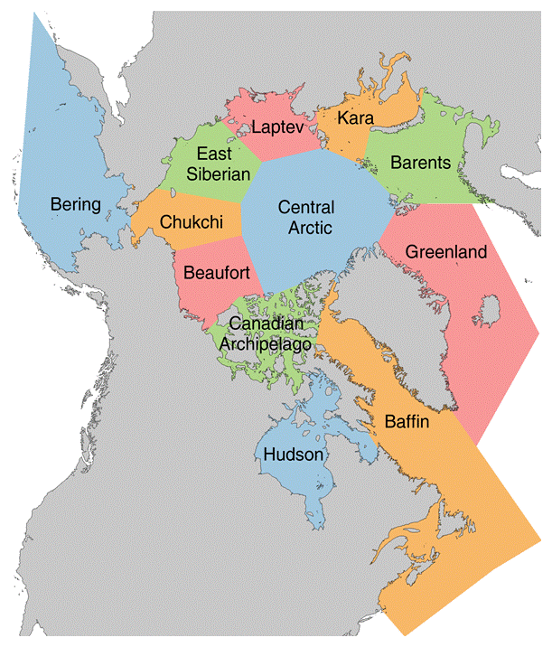
G10010 was used to compute the time series of monthly sea ice extent for the pan-Arctic domain and various Arctic subregions in which sea ice is at least a seasonal feature. The regionalization adopted here follows that of the MASIE (Multisensor Analyzed Sea Ice Extent) product available from the National Snow and Ice Data Center (http://nsidc.org/data/masie/browse_regions, last access: 27 December 2018). MASIE (NIC and NSIDC, 2010) regions are defined by the U.S. Navy–NOAA–U.S. Coast Guard National Ice Center (NIC) on the basis of operational analyses areas. We use the following MASIE regions: (1) Beaufort Sea, (2) Chukchi Sea, (3) East Siberian Sea, (4) Laptev Sea, (5) Kara Sea, (6) Barents Sea, (7) East Greenland Sea, (8) Baffin Bay/Davis Strait, (9) Canadian Archipelago, (10) Hudson Bay, (11) central Arctic Ocean and (12) Bering Sea. There are several other MASIE regions (Baltic Sea, Yellow Sea, Cook Inlet) that are not used here because they are not geographically connected with the main Arctic sea ice cover. Figure 1 shows the regions.

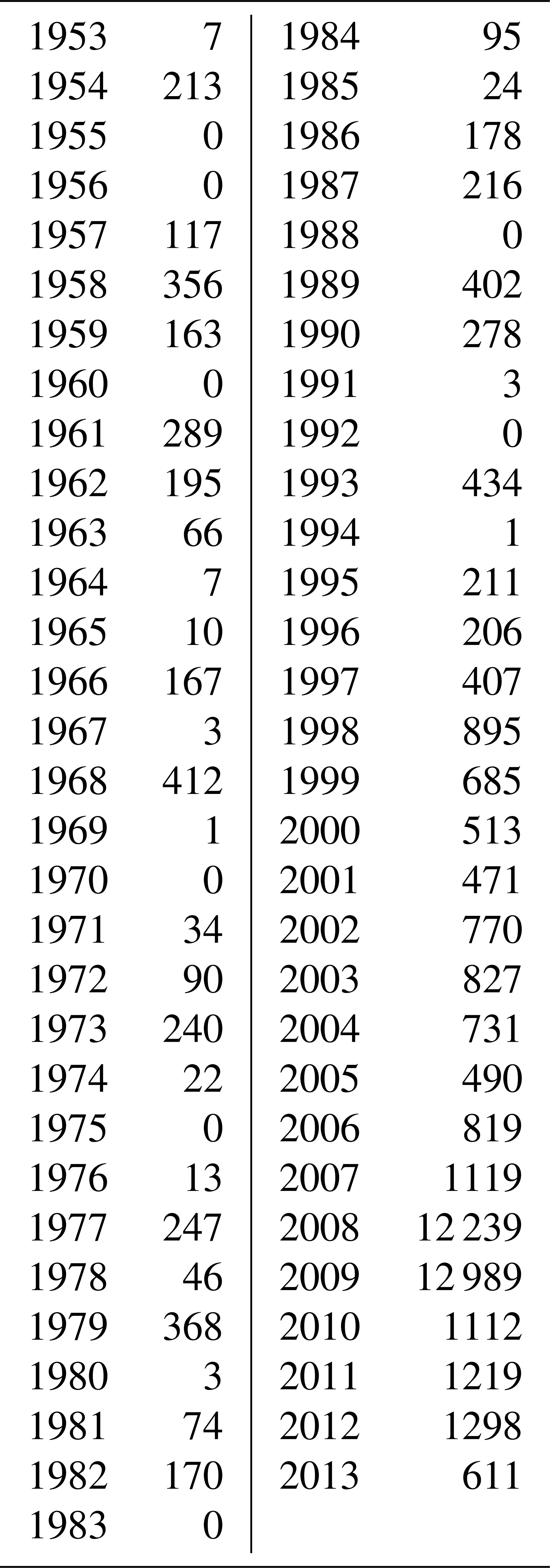
We also make use of the long ice extent record provided by G10010 to investigate the extent to which the Barnett Severity Index, or BSI, may be statistically predictable from antecedent ice extent. The BSI is directly relevant to offshore navigation applications in the Beaufort Sea. It is a metric of the severity of ice conditions, such as conditions encountered by barges resupplying the North Slope. The BSI is determined once per year, at the end of the summer shipping season, by analysts at the NIC. It is a unitless linear combination of five parameters: (1) the distance in nautical miles from Point Barrow northward to the ice edge on 15 September, (2) the distance from Point Barrow northward to the 50 % ice concentration line on 15 September, (3) the number of days the entire sea route from the Bering Strait to Prudhoe Bay is ice-free in a calendar year, (4) the number of days the entire sea route to Prudhoe Bay is less than or equal to 50 % ice concentration in a calendar year, and (5) the temporal length of the navigable season, defined as the time period from the initial date the entire sea route is less than 50 % ice concentration to 1 October (Barnett, 1980). Figure 2 is a time series of the BSI reconstructed from gridded sea ice concentration data (see Appendix). Higher values indicate less severe ice conditions.

Figure 1 The MASIE subregions used in the study (NIC and NSIDC, 2010).

Figure 2 Time series of the Barnett Severity Index (BSI), 1953–2013.

4 Methods

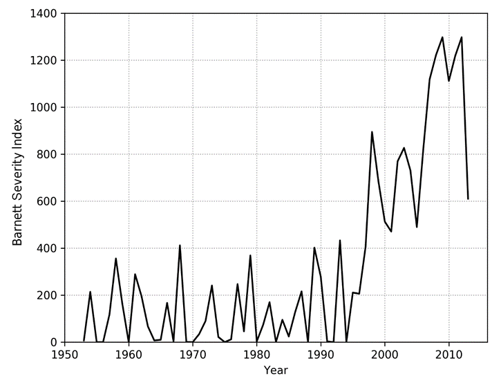
As shown in Fig. 3, Arctic sea ice extents have generally been decreasing over the post-1953 period of this study. The Beaufort Sea is a prime example of a region in which summer and autumn sea ice coverage has been decreasing, although winter (March) sea ice extent in the Beaufort Sea shows no trend or variability because the ice edge extends to the coastline in March of every year, essentially eliminating year-to-year variations. Consistent with the September decrease of Beaufort ice extent, the BSI has been increasing over the past few decades (Fig. 2). Two time series containing trends over time can show a correlation simply because the trends are present in the time series. A trend can be used as a predictive tool by assuming its continuation into the future. However, a trend can inflate persistence-based forecast skill when a variable is used to predict itself (assuming the historical trend continues into the future). Indeed, depictions of time variations of a quantity such as sea ice extent are often shown as departures from a trend line in order to highlight the interannual variations. One of our main interests in this study is whether or not interannual variations of preceding regional ice extents correlate with later BSI values. In order to exclude the effect of the overall trends in the correlation of these time series, we detrend the data and explore various methods for doing so.

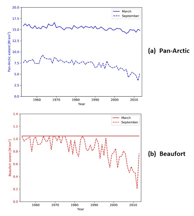
Figure 3 (a) Total Arctic sea ice extent and (b) the extent of ice in the Beaufort Sea during March (solid lines) and September (dashed lines).

The choice of a function with which to detrend the time series should be determined by features of the series itself. The detrended time series should exclude the general tendency to change over time but preserve a measure of the year-to-year variability of the series. The previous studies cited in Sect. 2 (e.g., Blanchard-Wrigglesworth et al., 2011; Sigmund et al., 2013; Day et al., 2014; Bushuk et al., 2017, 2018) have generally relied on least-squares linear fits, while Dirkson et al. (2017) suggested the use of a quadratic fit for detrending pan-Arctic sea ice area. Goldstein et al. (2016, 2018), by contrast, showed that discontinuous changes in the mean better captured time series (such as open water area) characterized by abrupt changes. In the spirit of the Goldstein et al. (2016, 2018) studies, we explore various options for detrending a time series such as those in Figs. 2 and 3, for which the changes are more pronounced in recent decades than in earlier decades. In such cases, a single multi-decadal trend line cannot be expected to optimally represent the historical evolution.

We explored several functional forms that fit the time series, including linear, quadratic, cubic, and exponential functions. We found that a simple two-piece linear function – wherein the data are modeled by two line segments that intersect at a break-point year – had the lowest average root-mean-square (rms) difference between the time series and the fitted function, although fits using other functions had only slightly larger rms differences. This choice of the detrending fit has the additional feature of giving a sense of when the ice extent began to change more rapidly.

The two-piece linear fits were obtained by using standard statistical algorithms. A function defined by two intersecting half-lines can be specified by the coordinates of one point on each half-line and the intersection point. With the x axis as time, and the y axis as the value of the sea ice extent, the x values of the non-intersecting points can be chosen to be 1953 and 2013, the first and last years of the BSI dataset. This leaves four values for the function to fit: the series value in 1953, the series value in 2013, and the year and value at the intersection point, also referred to here as the break point. We note that the break point is not specified by the user but is determined by the algorithm so that the fit to the time series is optimized. The “curve_fit” method is defined in lines 504–794 of the file https://github.com/scipy/scipy/blob/master/scipy/optimize/minpack.py (last access: 24 March 2019). This method performs a least-squares fit to the function by modifying the equation's parameters. A starting “guess” of the equation parameters is provided by the user. The curve_fit method of the SciPy numerical library is then used to algorithmically modify the equation parameters to find the best two-piece linear fit to the function.

In Fig. 4, we show the piecewise linear fit together with quadratic, cubic, and exponential fits to the time series of the BSI and the September Beaufort Sea ice extent. In the case of the two-piece linear fit, the break point – found by the curve_fit procedure to best fit the data – is in the early 1990s for both sea ice metrics. It is visually apparent from Fig. 4 that all four fits are comparable in terms of the overall magnitudes of the departures from the trend lines. The rms departures from the various trend lines indeed differed by less than 10 %. Because the two-piece linear fit was usually the best fit and also provided a clear estimate – the break-point year – of when the recent rate of sea ice loss accelerated, we chose the two-piece linear for the remainder of this study. The break points are computed separately for each region, allowing the use of the two-piece linear fit to compare the timing of the change in ice loss rate among the various subregions.

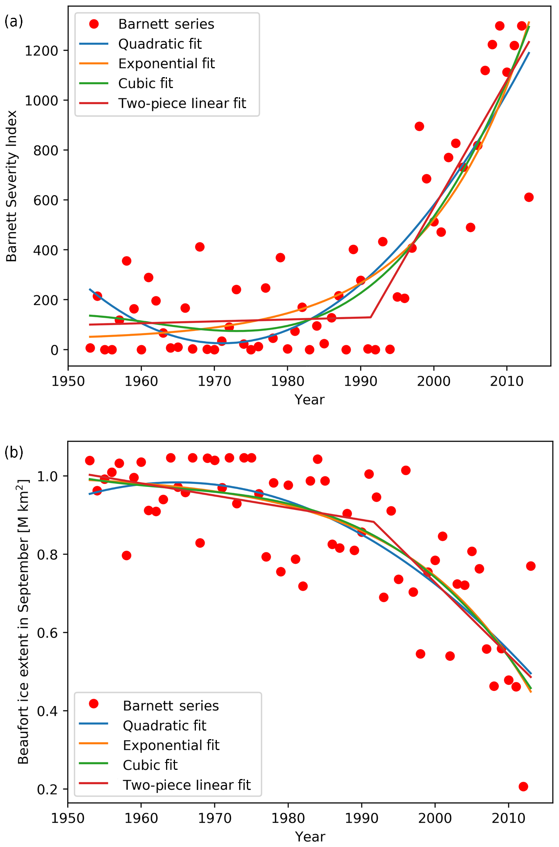
Figure 4 Examples of different fit methods (see legend) applied to the BSI (a) and the September Beaufort ice extent time series (b).

After using the curve_fit method to find two-piece linear fits to the BSI and the regional and pan-Arctic sea ice extent time series, we subtracted this linear fit from the original data to get a detrended time series for each sequence. We were then able to use the “linregress” method from the SciPy (Jones et al., 2001) software library to find the linear relationship between the detrended regional monthly extent values and both the detrended BSI and the detrended pan-Arctic extent. We then used the “stats” method from SciPy to compute the square of the Pearson correlation coefficient (R²) and the p value estimate of statistical significance for this relationship.

5 Results

As noted in Sect. 2, previous studies (Bushuk et al., 2018) have evaluated the persistence of regional ice extent over the post-1978 period of satellite observations. Here we extend this evaluation to encompass a longer period dating back to 1953 in order to assess the stability of the persistence statistics. Specifically, for each region in Fig. 1, we have correlated the September ice extent with the ice extent of antecedent months for the 1953–2013 and 1979–2013 periods. Figure 5 compares these persistence values (autocorrelations at multi-month lags), for the antecedent months of March, May, and July in a subset of regions. Because the regions chosen were those that have interannually varying ice cover in September, regions such as the Bering Sea, Hudson Bay, the Sea of Okhotsk, and the Baltic Sea were excluded. The correlations for the non-detrended and detrended ice extents are shown in panels (a) and (b), respectively.

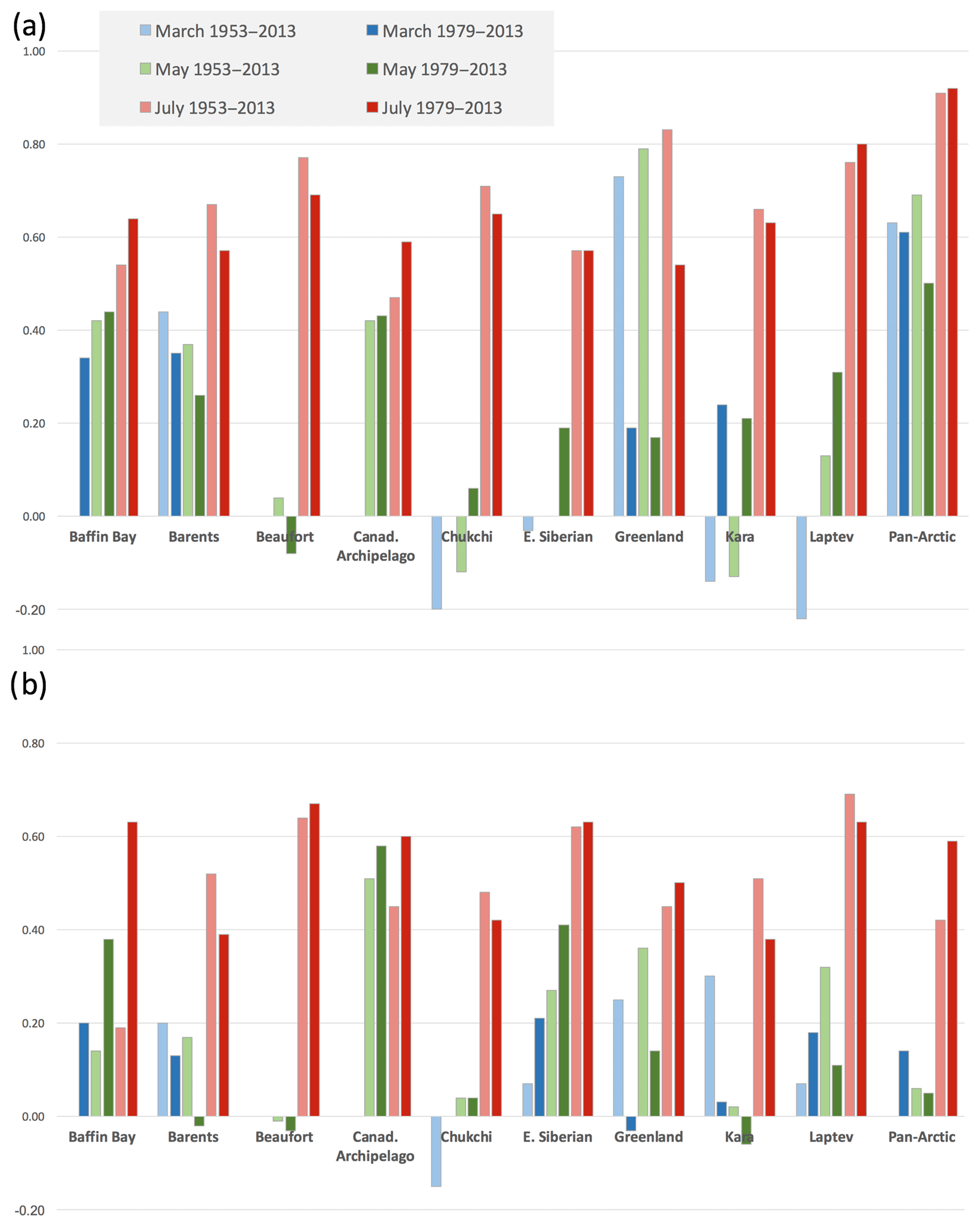
Figure 5 Correlations of September ice extents in individual seas with ice extent in the same region in March (green bars), May (blue bars), and July (red bars) bases on (a) non-detrended data and (b) detrended data. Correlations are also shown for Pan-Arctic extent (far right in each panel). The correlations are based on non-detrended data. For each color, light-colored bars are for 1953–2013 and dark-colored bars are for 1979–2013. The absence of a bar indicates a correlation of zero. The 95 % significant levels for the longer and shorter samples are 0.26 and 0.33, respectively.

For most of the regions, the inclusion of the earlier decades does not have a notable impact on the persistence from July to September, and detrending the data does not change this conclusion. However, in the non-detrended results of Fig. 5a, the March–September and May–September correlations change substantially in a few regions. The Baffin Bay March–September correlations increase from 0.00 to 0.34 when the earlier decades are eliminated, largely as a result of the post-1979 trend: the post-1979 correlation is statistically significant (p<0.05) based on a Wald test with t distribution of the test statistic and a two-sided p value for a null hypothesis that the slope is zero. The pan-Arctic correlations, as Fig. 5a shows, are higher than the correlations for the individual regions and also increase when the earlier decades are eliminated. In the Greenland Sea, the correlations from March and May decrease substantially and lose statistical significance when the earlier decades are eliminated.

As shown in Fig. 5b, the detrending generally reduces the magnitudes of the correlations between September and the earlier months, both for the longer post-1953 periods and the shorter post-1979 periods: the March–September correlations based on the detrended data for the longer/shorter periods are −0.05/0.20 for Baffin Bay, 0.20/0.13 for the Barents Sea, 0.00/0.00 for the Beaufort Sea (no March variance), 0.00/0/00 for the Canadian Archipelago (no March variance), −0.15/0.00 for the Chukchi Sea, 0.07/0.21 for the East Siberian Sea, 0.25/−0.03 for the Greenland Sea, 0.03/0.03 for the Kara Sea, and 0.07/0.18 for the Laptev Sea. The corresponding 5 % significant levels are 0.26/0.33. Except for the Canadian Archipelago and East Siberian regions, the May–September correlations in Fig. 5b are also small (<0.40). Only the July–September correlations are above 0.40 in all regions for the detrended data. In view of generally small magnitudes of the March-September and May–September correlations in Fig. 5b, we conclude that the springtime “predictability barrier” (Lindsay et al., 2008; Day et al., 2014; Bushuk et al., 2018) in regional forecasts based on persistence of ice extent anomalies is not reduced by the inclusion of several decades of pre-satellite data.

Figure 6 The distribution of break-point years across all regions for (a) January–September and its three subperiods: (b) January–March, (c) April–June, and (d) July–September. Only cases for which detrending using two lines, rather than one, reduced the rms error by 5 % or more are included. Note that y axes have different scales.

Because changes of trend have not been addressed systematically in previous evaluations of Arctic sea ice trends, we synthesized the break-point information across all regions and calendar months (January–September) included in our study. The synthesis was limited to only those regions and calendar months in which the two-piece linear fit reduced the rms residual by at least 5 % relative to the one-piece linear best fit. Figure 6 groups the break points into 5-year periods ending in 1955, 1960, ..., 2015. In order to capture the seasonality of the break points, we present separate plots for (a) the entire January–September period, (b) January–March (winter), (c) April–June (spring), and July–September (summer). As shown in panel (a), nearly all the break points occur in the second half of the study period, with a maximum in 1991–1995. The 1991–1995 period has the most break points of any 5-year period, and the 1990s have nearly as many break points as all the other decades combined. The small secondary peak in the 1960s represents eight break points scattered across the regions and seasons (Cook Inlet in January and February, East Siberian Sea in February and April, pan-Arctic in July, Hudson Bay in August, Baffin-St. Lawrence and Bering in September), showing no systematic pattern that would suggest a meaningful signal. The winter and summer seasons are the primary contributors to the maximum in the 1990s, as the spring break points are evenly distributed through the latter half of the study period. However, spring has the fewest (12) break points overall, while the summer has the most (26). The break points for our focal metrics, the BSI and September pan-Arctic ice extent, are 1991 and 199, respectively, consistent with the distribution in Fig. 6. These two metrics are included in the results summarized in Fig. 6. One may conclude that the 1990s, and to a lesser early 2000s, represent the shift to a more rapid rate of sea ice loss. If one is to argue for a “regime shift” in Arctic sea ice loss (Lenton, 2012), this period would be the leading candidate.

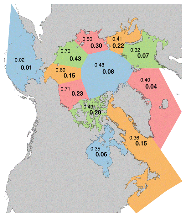
Figure 7 Squares of correlations (R²) between September pan-Arctic ice extent and September regional ice extent based on ice extents including trends (upper numbers in normal font) and detrended (lower numbers, bold font). The 95 % significance thresholds for the correlations range from 0.26 with no autocorrelation (generally the case for detrended data) to 0.38 with an autocorrelation of 0.4; the corresponding R² thresholds are 0.07 and 0.14.

In order to illustrate the effect of the detrending and to show which regions contribute the most explained variance to pan-Arctic sea ice extent, Fig. 7 shows the squares of the correlations (R²) between September pan-Arctic ice extent and the concurrent ice extent in each of the subregions. The figure shows values of R² before detrending (upper numbers, regular font) and after detrending (lower numbers, bold font). With the trend included, the R² values are relatively high in most regions (except for the Bering Sea), ranging from 0.32 to 0.71; the corresponding correlations (R) range from 0.57 to 0.84. Based on the t test described earlier, these correlations all exceed the 95 % significance thresholds, which range from 0.26 (R²=0.07) for a 60-year sample with no autocorrelation to 0.38 (R²=0.14) for a 60-year sample with an autocorrelation of 0.4. None of the regional or pan-Arctic ice extent autocorrelations exceeded 0.40. Because these correlations are dominated by the trend, the larger values appear in the regions with trends that are most similar to the pan-Arctic trend. When the data are detrended, the explained variances are much smaller (R² values in bold font in Fig. 7) although still larger than the 95 % significance thresholds for a 60-year sample (R=0.26, R²=0.07). These smaller values indicate the relative contributions of regional variations to the interannual variations of pan-Arctic ice extent. According to Fig. 7, the regions contributing most strongly to September pan-Arctic sea ice variations (including trends) are the Beaufort, Chukchi, and East Siberian seas. After the data are detrended, the regions contributing most to September pan-Arctic sea ice variations are the East Siberian and Laptev seas. The relatively large contribution of the Laptev Sea is consistent with the “dynamical preconditioning” hypothesis of Williams et al. (2016). The variances of the detrended pan-Arctic September extents explained by the East Siberian and Laptev seas are indeed among the largest of all the regions, although the Chukchi Sea's interannual variance is essentially as large.

Figure 8 shows the squares of the correlations between the annual BSI and regional September ice extent before the detrending of both variables (top numbers) and after detrending (bottom numbers). While the actual correlations between the BSI and regional extent are generally negative, the R² values plotted in Fig. 8 are positive. Large values of R² appear in most regions when the trend is included (upper numbers) because the BSI has a strong positive trend over time, while September ice extent in most regions has a negative trend. The R² values are much weaker in regions away from the Beaufort Sea when the trends are removed (lower numbers in Fig. 8). The detrended R² values show the spatial representativeness of the BSI as a measure of interannual variations in each region. Figure 8 shows that the regions of significant explained variance include the Canadian Archipelago to the east as well as the Chukchi Sea to the west. However, the “scale of influence”, if measured by the area of significant correlation, is smaller for the BSI in Fig. 8 than for pan-Arctic ice extent in Fig. 7.

Table 1 Correlations between monthly regional ice extent and pan-Arctic ice extent expressed as explained variance (R²). Cases in which at least 10 % of the variance in pan-Arctic ice extent is explained by regional ice extent in a given antecedent month are highlighted with bold region names. Levels of shading of boxes denote values exceeding 0.10, 0.20, 0.30, etc.

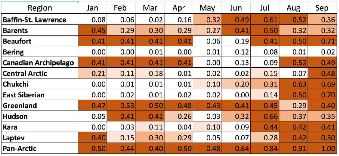
Table 2 Correlations between detrended monthly regional ice extent and detrended September pan-Arctic ice extent expressed as explained variance (R²). Cases in which at least 10 % of the variance in September pan-Arctic ice extent is predictable by regional ice extent in a given antecedent month are highlighted with bold region names. Shading of boxes is as in Table 1.

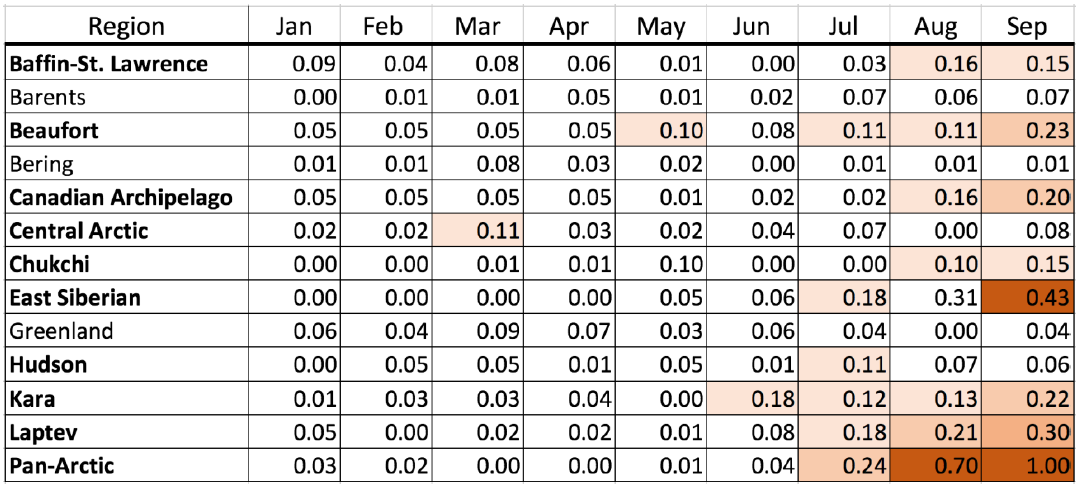
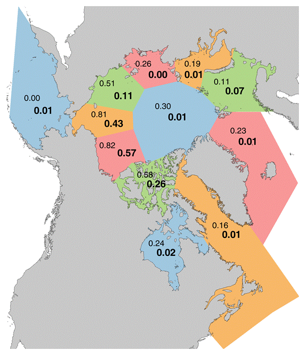
Figure 8 As in Fig. 7, but for squares of correlations between the annual BSI and September regional ice extents based on raw (not detrended) time series (upper numbers) and detrended time series (lower numbers, bold font). The 95 % significance thresholds for the R² values range from 0.07 with no autocorrelation (generally the case for detrended data) to 0.14 with an autocorrelation of 0.4.

Because the potential for seasonal predictions is a key motivation for this study, we examine cross-correlations in which the predictands (pan-Arctic ice extent and the BSI) lag potential predictors (regional ice extents) by intervals ranging from zero (no lag) to several seasons. Cross-correlations between non-detrended and detrended September pan-Arctic and regional ice extents are summarized in Tables 1 and 2 respectively. Cross-correlations between the BSI and regional ice extents (not shown) decreased similarly when the data were detrended. In all cases, the numerical values are the R² values. In order to illustrate the contribution of the trend to the apparent forecast skill, we present these correlations graphically for the regions which show the strongest associations with the September predictands. Figure 9 shows the R² values for cases in which September pan-Arctic ice extent lags by 0, 1, 2, ..., 8 months the ice extent in five subregions: the Beaufort, Chukchi, East Siberian, Barents, and Laptev seas. The red bars correspond to correlations computed from the data with the trends included. Not surprisingly, the R² values are largest at zero lag. The rates at which the correlations decrease with increasing lag vary regionally, reaching zero by 3–4 months for the Beaufort, Chukchi, and East Siberian seas. The zero-month lag values are quite large for the Beaufort, Chukchi, and East Siberian regions, where they exceed R²=0.7 (R=0.84).

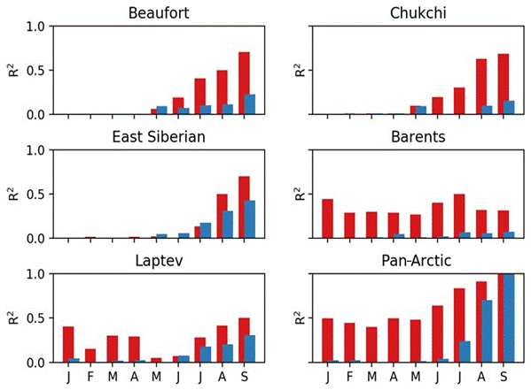
Figure 9 Examples of variances of September pan-Arctic ice extent explained by correlations with antecedent regional ice extent in individual calendar months from September back to January (pan-Arctic extent lagging by 0, 1, 2, ..., 8 months). Plotted values are squares of correlations (i.e., explained variances). Red bars are values with trends included, and blue bars are squared correlations after removal of trends. The 95 % significance thresholds for the R² values range from 0.07 with no autocorrelation (generally the case for detrended data) to 0.14 with an autocorrelation of 0.4.

However, after detrending (using the two-piece linear best fits), most of the apparent forecast skill is lost. As shown by the blue bars in Fig. 9, nearly all the predictability from the Barents and Chukchi seas vanishes with the detrending, while only small fractions of explained variance remain at non-zero lags when sea ice extents for the Beaufort and East Siberian seas are the predictors. For example, when the regional extent leads by two months (July), the fractions of explained variance are approximately 0.16 and 0.10 (R∼0.40 and 0.32) for the East Siberian and Beaufort seas, respectively. The implication is that the persistence of interannual variations about the trend line makes only small contributions to interannual variations of pan-Arctic sea ice extent and that these small contributions result mainly from the Pacific sector of the Arctic. As indicated by Fig. 9, the pan-Arctic extent of July and August correlates more highly than any regional extent with September pan-Arctic ice extent in both the non-detrended and the detrended data (see also Tables 1 and 2).

The lagged R² values relevant to predictions of the Barnett Severity Index are shown in Fig. 10. Because the BSI is based primarily on ice conditions in the Beaufort Sea in August and September, it is not surprising that the correlation is largest for the Beaufort's ice extent in September, when the R² value is approximately 0.8 for data that are not detrended. The August and September values for the Chukchi are essentially as large as the corresponding Beaufort values, indicating a spatial coherence of the variations (with trends included) in the two regions. The antecedent extents in the East Siberian and Barents regions also explain statistically significant fractions of the variance when the trends are included.

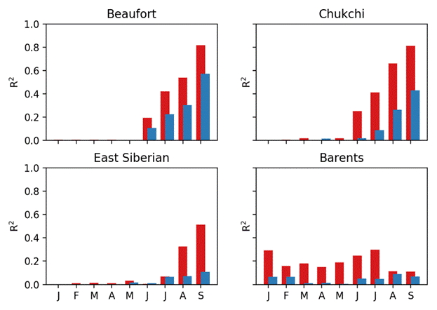
Figure 10 Examples of variances explained by correlations between the Barnett Severity Index and regional ice extent in individual calendar months from September back to January (BSI lagging by 0, 1, 2, ..., 8 months). Plotted values are squares of correlations (i.e., explained variances). Red bars are values with trends included, and blue bars are squared correlations after removal of trends. Significance thresholds as in Fig. 9.

The blue bars in Fig. 10 are the lagged R² values based on the detrended data. Because the trend's contribution to the forecast skill has been removed, these correlations provide the most meaningful assessment of the seasonal forecast skill if the BSI based on antecedent ice conditions. The largest correlations are for the Beaufort Sea, where the explained variances decrease from about 0.55 (R∼0.74) in September to about 0.10 (R∼0.32) in June. The correlations for the Chukchi are only slightly smaller, but the BSI variance explained by all other regions is less than 10 %. The percentage of variance explained by the antecedent ice extent of the nearby regions (Beaufort, Chukchi, East Siberian seas) is less than one might have anticipated, given that the BSI includes information on the length of the navigation season, which can begin well before September, i.e., as early as July in some years.

While the results presented here imply that the persistence of detrended sea ice anomalies provide only limited forecast skill, a key question is the following: how much better are sea ice forecasts based on other approaches? The Sea Ice Prediction Network's Sea Ice Outlook (SIO) consists of seasonal forecasts of September sea extent based on a variety of approaches (numerical modeling, statistical, and heuristic) on an annual basis beginning in 2008. In most years, several dozen individual (or groups) provide the SIO with data based on September sea ice extent prediction and other information available at the end of May, June, and July. A compilation of SIO results from 2008 to 2018 enables a quantitative comparison of the skill of the SIO and persistence-based forecasts. (In this case, persistence was evaluated from the mean ice extents in the National Snow and Ice Data Center's G02135_v3.0: ftp://sidads.colorado.edu/DATASETS/NOAA/G02135/seaice_analysis/, last access: 27 December 2018.) The median absolute error of the all-forecaster average SIO issued in July of 2008–2018 is 0.32 million km², while the corresponding median absolute error of forecasts of persistence of the departure from the trend line of the pan-Arctic ice extents of May, June, July, and August are 0.43, 0.22, 0.25, and 0.09 million km². Thus the SIO forecasts issued in July outperform the trend-line anomaly persistence forecasts from May, but not from June, July, or August. Persistence of the previous September's deviation from the trend line has a median absolute error of 0.37 million km², while simple persistence of the previous year's actual value has an error of 0.40 million km². The corresponding rms errors (in millions of square kilometers) are 0.57 for SIPN; 0.67, 0.46. 0.42, and 0.18 for persistence of the trend-line departures of May, June, July, and August; 0.68 for persistence of the trend-line departure from the previous September; and 0.67 for persistence of the actual extent from the preceding September. The SIO forecasts used in this comparison were averages of all forecasts submitted to SIO, so it is quite possible that some individual forecasters participating in the SIO perform considerably better. Nevertheless, it is apparent that sea ice anomaly persistence is a challenging control forecast and a respectable competitor for forecasts issued by the scientific community

6 Conclusion

The substantial decrease of Arctic sea ice over the past several decades is well documented (Cavalieri and Parkinson, 2012; Parkinson, 2014; Serreze and Stroeve, 2015; Onarheim et al., 2018). Of all the regions considered here, only the Bering Sea does not show a negative trend, and the Bering trend is only positive in January–April (Onarheim et al., 2018, their Table 1). Moreover, the extreme minima of Bering Sea ice during the past two winters (2016–2017 and 2017–2018) are starting to bring the Bering's trend into alignment with the other regions of the Arctic.

The prominence of the trends in the time series of regional as well as pan-Arctic ice extent makes it important to distinguish the contribution of the trend from other sources of forecast skill. In this study we explored the use of several methods of detrending in order to evaluate the use of ice anomaly persistence (autocorrelation) and regional cross-correlations as predictors of ice variations. The two-piece linear trend evaluations generally have break points in the 1990s, indicating that the rate of ice loss has been greater in the past two decades than in the earlier portion of the satellite era that began in 1979.

Based on the raw (not detrended) time series, the antecedent ice extents in a substantial fraction of the Arctic regional seas explain statistically significant fractions of variance of September pan-Arctic ice extent and also of the Barnett Severity Index, which is more specific to the Beaufort Sea. Statistically significant portions of variance of both September metrics are explained by the regional ice extents of prior seasons. However, this predictive “skill” is attributable primarily to the trends in the data. Removal of the trend leaves little forecast skill beyond a month or two when the forecast method is limited to the relatively simple statistical correlations utilized here. The low persistence-derived skill for the detrended September pan-Arctic ice extent is consistent with the findings of Stroeve et al. (2014) based on the Sea Ice Outlook as part of the Study of Environmental Arctic Change (SEARCH). Moreover, our inclusion of data back to the early 1950s shows that the springtime predictability barrier in regional forecasts based on persistence of ice extent anomalies is not reduced by the inclusion of several decades of pre-satellite data.

It must be noted that other sea ice prediction approaches have outperformed persistence (e.g., Tivy et al., 2007; Schröder et al., 2014; Yuan et al., 2016; Petty et al., 2017; Bushuk et al., 2018). Some of these studies have used statistical methods informed by other predictors (e.g., Lindsay et al., 2008; Tivy et al., 2011), some have used the perfect model approach (e.g., Blanchard-Wrigglesworth et al., 2011), and some have made use of initialized hindcasts (e.g., Bushuk et al., 2018). Nevertheless, persistence-derived skill provides a baseline for the measurement of forecast skill achieved by these other approaches, and, based on the results in Sect. 5, persistence of departures from the trend lime can be a challenging competitor at forecast ranges of months to seasons.

While the variance explained by simple anomaly persistence at lead times of several seasons and also by persistence of detrended anomalies at lead times of a month or two is statistically significant, statistical significance does not equate to usefulness. Potential users of sea ice forecasts include local communities engaging in offshore subsistence and travel activities, marine transport companies, offshore resource extraction, and the tourism industry. The relatively small fractions of variance predictable several months in advance using detrended data (Figs. 6–9) will likely leave uncertainties that are too great for many users. However the trend-derived skill, which can represent 50 % or more of the variance, may enable decisions if the interannual variations superimposed on the trend represent acceptable risks for users of sea ice forecasts.

Appendix A: Reconstruction of the Barnett Severity Index, 1953-2013

As described in Sect. 2, the Barnett Severity Index (BSI) is a combination of five metrics of ice coverage in the Beaufort Sea. Drobot et al. (2006) used the BSI through 2000 in their evaluation of predictability based on multilinear regression against various measures of sea ice cover. In order to update the BSI for use in this study, we base a reconstruction on the digital grids of sea ice concentration in the Historical Sea Ice Atlas (HSIA) for Alaska (http://seaiceatlas.snap.uaf.edu/, last access: 13 March 2019). As with the regional ice extent calculations using G10010 (Sect. 3), we use the HSIA because it extends the record 26 years back in time before the start of the satellite passive microwave record. While the sources of the ice concentration data in the HSIA are the same as in G10010, a notable advantage of the HSIA is its weekly temporal resolution (vs. the monthly resolution of G10010). The HSIA also has a spatial resolution of 1∕4^∘ latitude by 1∕4^∘ longitude. Because of the weekly time resolution, the distance metrics (3)–(5) of the BSI are truncated to the nearest week. Similarly, the distance metrics (1) and (2) are truncated to the nearest 27.8 km (15 nmi, nautical miles). One of the within-month dates of the HSIA grids is the 15th of each month, so no temporal interpolation is necessary for metrics (1) and (2). The reconstructed values of the BSI are listed in Table A1.

Table A1 Yearly values of the Barnett Severity Index (BSI). Source: Rebecca Rolph, Geophysical Institute, University of Alaska, Fairbanks.