Effects of short-term variability of meteorological variables on soil temperature in permafrost regions

Effects of the short-term temporal variability of meteorological variables on soil temperature in northern high-latitude regions have been investigated. For this, a process-oriented land surface model has been driven using an artificially manipulated climate dataset. Short-term climate variability mainly impacts snow depth, and the thermal diffusivity of lichens and bryophytes. These impacts of climate variability on insulating surface layers together substantially alter the heat exchange between atmosphere and soil. As a result, soil temperature is 0.1 to 0.8 ^∘C higher when climate variability is reduced. Earth system models project warming of the Arctic region but also increasing variability of meteorological variables and more often extreme meteorological events. Therefore, our results show that projected future increases in permafrost temperature and active-layer thickness in response to climate change will be lower (i) when taking into account future changes in short-term variability of meteorological variables and (ii) when representing dynamic snow and lichen and bryophyte functions in land surface models.

1 Introduction

Soil temperature is an important physical variable of a terrestrial ecosystem since it controls many functions of microbes and plants. In permafrost regions, soil temperature also defines the biologically active part of the soil that is thawing in summer (active layer). Therefore, impacts of future warming on soil temperature have been investigated in numerous experimental and modelling studies during the past decades. Large-scale soil temperature is mainly determined by vertical heat conduction. Therefore, soil temperature usually follows an annual sinusoidal cycle of air temperature with a damped oscillation (Campbell and Norman, 1998). That is why the projected large increase in air temperature in the Arctic region over the next 100 years (Ciais et al., 2013) is raising large concerns about the response of soil temperature and hence permafrost thawing in the Arctic. Indeed, measurements during the last decades already show an increasing permafrost temperature (Romanovsky et al., 2010) and active-layer thickness (Callaghan et al., 2010) in response to global warming. Also, initial modelling results confirm such simple response of increasing future soil temperature and active-layer thickness (Koven et al., 2011; Schaefer et al., 2011; Lawrence et al., 2012; Peng et al., 2016). As a result of increasing soil temperature and active-layer thickness, heterotrophic respiration is suggested to increase because of the temperature response of biochemical functions (Arrhenius, 1889; van't Hoff, 1896; Lloyd and Taylor, 1994) and the additional availability of decomposable substrate (Schaphoff et al., 2013; Koven et al., 2015) potentially leading to a positive climate–carbon cycle feedback (Zimov et al., 2006; Beer, 2008; Heimann and Reichstein, 2008).

Meteorological variables, such as air temperature and precipitation, will not only change gradually into the future, but also their short-term variability and frequency of extreme events is projected to change (Easterling et al., 2000; Rahmstorf and Coumou, 2011; Seneviratne et al., 2012). For instance, for northern high-latitude regions, climate models project an increase of the annual maximum of the daily maximum temperature by 4 ^∘C by 2100 (Seneviratne et al., 2012) while annual maximal daily precipitation is projected to increase by 20 % in these areas by 2100. At the same time, many ecosystem functions respond non-linearly to environmental factors; cf. for instance the temperature-dependence of biochemical functions (Arrhenius, 1889). Therefore, effects of the short-term (daily to weekly) variability of meteorological variables on the long-term (decadal) mean ecosystem functions can enhance or dampen the effect of a general gradual warming (Reichstein et al., 2013; Schwalm et al., 2017). That is why there is a strong need to understand such effects of climate variability on ecosystem states and functions in addition to gradual changes in order to reliably project future ecosystem state dynamics and climate. In this context, effects of climate variability on soil temperature in northern high-latitude environments have not been studied so far: In addition to a gradual warming of Arctic air and soil temperature, what are the specific effects of changing short-term variability of meteorological variables on the long-term mean annual or seasonal soil temperature? Will a short-term variability change have the capability to enhance or dampen the anticipated soil warming?

Due to the well-known dampening effects of snow, near-surface vegetation and the organic layer (Yershov, 1998, pp. 361–369) (Goodrich, 1982; Zhang, 2005; Jafarov and Schaefer, 2016; Wang et al., 2016), one would expect no to little additional effects of changing air temperature fluctuations on soil temperature, in particular on subsoil and permafrost temperature. However, air temperature variability will have an impact on snow height indirectly through snow density (Abels, 1892) and also directly when temperature periodically rises above the melting point. In addition, the dependence of soil and near-surface vegetation conductivity on water and ice content (Campbell and Norman, 1998) complicates the picture because water and ice contents themselves are also temperature-dependent. Snow manipulation experiments have proven the large spatial heterogeneity of soil temperature in cold regions due to snow height heterogeneity (Wipf and Rixen, 2010). The temporal variability of insulating layers and their properties should be of similar importance for soil temperature.

At high latitudes, near-surface vegetation consists to a large extent of lichens and bryophytes, which often form a continuous layer on the ground. Lichens are symbiotic organisms consisting of a fungus and at least one green alga or cyanobacterium, while bryophytes are non-vascular plants which have no specialized tissue such as roots or stems. Both groups cannot actively control their water uptake or loss, but they tolerate drying and are able to reactivate their metabolism on rewetting. Typical species of upland regions at high latitudes are feather bryophytes such as Hylocomium splendens and Pleurozium schreberi or the lichen Cladonia stellaris. This near-surface vegetation grows on top of any organic horizon and is hence important for heat fluxes between land and atmosphere. In particular also for this layer, thermal and hydrological properties depend highly on water and ice content. Hence, lichens and bryophytes dynamically influence the vertical heat conduction (Porada et al., 2016a).

This study investigates the effects of temporal variability of meteorological variables on snow and lichen/bryophyte insulating properties and hence soil temperature in permafrost regions. For this, a recently advanced land surface model (LSM) has been used that also represents permafrost-specific processes, and in particular a dynamic snow representation and a dynamic near-surface vegetation model (Porada et al., 2016a). While the model has been evaluated against several types of observations in other studies (Ekici et al., 2014, 2015; Porada et al., 2016a; Chadburn et al., 2017), here mean annual ground temperature (MAGT) is evaluated again against different observations or other modelling studies. Then, the model is run with two distinct climate forcing datasets, one control dataset and one that has identical long-term averages but reduced day-to-day variability of meteorological variables, such as air temperature and precipitation. The differences in long-term average results from these two model runs will therefore demonstrate the exclusive effects of temporal variability of climate variables and extreme meteorological events on MAGT in high-latitude permafrost regions.

2 Methods

2.1 The land surface model JSBACH

The Jena Scheme for Biosphere–Atmosphere Coupling in Hamburg (JSBACH) is the land surface scheme for the Max Planck Institute Earth System Model (MPI-ESM) (Raddatz et al., 2007; Reick et al., 2013). It runs coupled to the atmosphere inside the ESM or offline forced by observation-based or projected climate input data. This model has recently been advanced by several processes which are particularly important in cold regions (Ekici et al., 2014): coupling of soil hydrology and heat conduction via latent heat of fusion and the effects of soil ice and water content on thermal properties, and a snow model for soil insulation. The model simulates heat conduction and soil hydrology in a 1-D vertical scheme using several layers (Hagemann and Stacke, 2015). The version used in this study has been updated from the one used in Ekici et al. (2014) by two additional deep soil layers for thermal and hydrological processes of 13 and 30 m, respectively, which lead to a total potential soil profile of 53 m. However, soil hydrological processes are constrained by the depth to the bedrock. Another constraint on soil hydrological processes is the potentially available pore volume, which is reduced by ice content.

In contrast to the model version described in Ekici et al. (2014), here we use a further advanced snow module that includes dynamic snow density and snow thermal properties (Ekici, 2015). In this approach, the snow density (ρ_snow) follows a similar representation to that in Verseghy (1991). It is initialized with a minimum value of ${\mathit{\rho }}_{\text{min}}=\mathrm{50}\mathrm{kg}{\mathrm{m}}^{-\mathrm{3}}$. Then the compaction effect is included as a function of time and a maximum density (${\mathit{\rho }}_{\text{max}}=\mathrm{300}\mathrm{kg}{\mathrm{m}}^{-\mathrm{3}}$) value (Eq. 1),

$$\begin{array}{}\text{(1)}& {\displaystyle }{\displaystyle }{\mathit{\rho }}_{\text{snow}}^{t+\mathrm{1}}=\left({\mathit{\rho }}_{\text{snow}}^t-{\mathit{\rho }}_{\text{max}}\right)\exp {\displaystyle \frac{-\mathrm{0.002}\cdot \mathrm{\Delta }t}{\mathrm{3600}}}+{\mathit{\rho }}_{\text{max}},\end{array}$$

where Δt is the time step length of model simulation. Additionally, when there is new snowfall, snow density is updated by taking a weighted average of fresh-snow density (ρ_min) and the calculated snow density value of the previous time step.

Snow density controls snow heat conduction parameters. Equations (2) and (3) show the relationships of volumetric snow heat capacity (c_snow) and snow heat conductivity (λ_snow) to snow density following the approach of Abels (1892) and Goodrich (1982). With no previous snow layers, c_snow is initialized with an average value of $\mathrm{0.52}\mathrm{MJ}{\mathrm{m}}^{-\mathrm{3}}{\mathrm{K}}^{-\mathrm{1}}$ and λ_snow with $\mathrm{0.1}\mathrm{W}{\mathrm{m}}^{-\mathrm{1}}{\mathrm{K}}^{-\mathrm{1}}$,

$$\begin{array}{}\text{(2)}& {\displaystyle }{\displaystyle }{c}_{\text{snow}}=c_{\text{ice}}\cdot {\mathit{\rho }}_{\text{snow}},\end{array}$$

where c_ice is the specific heat capacity of ice $\left(\mathrm{2106}\mathrm{J}{\mathrm{kg}}^{-\mathrm{1}}{\mathrm{K}}^{-\mathrm{1}}\right)$, and

$$\begin{array}{}\text{(3)}& {\displaystyle }{\displaystyle }{\mathit{\lambda }}_{\text{snow}}=\mathrm{2.9}\times {\mathrm{10}}^{-\mathrm{6}}\cdot {\left({\mathit{\rho }}_{\text{snow}}\right)}^{\mathrm{2}}.\end{array}$$

Another important advancement of the JSBACH model version used in this study is the inclusion of a dynamic lichen and bryophyte model (Porada et al., 2013, 2016a). This model is designed to predict lichen and bryophyte net primary productivity (NPP) in a process-based way from available light, surface temperature, atmospheric carbon dioxide concentration, and water content of lichens and bryophytes. Furthermore, it is applicable when estimating various impacts of lichens and bryophytes on biogeochemical cycles (Lenton et al., 2016; Porada et al., 2016b, 2017). The model includes a dynamic representation of the surface cover which depends on the balance of growth due to NPP and reduction by disturbance, such as fire (Porada et al., 2016a). The coverage of the layer determines its influence on heat exchange between atmosphere and soil. The layer thickness and porosity are set to 4.5 cm and 80 %, respectively.

The lichen and bryophyte water balance is integrated into the scheme of hydrological fluxes in JSBACH. In addition, the lichen and bryophyte layer is fully integrated into the heat conduction scheme and hence also functions as a soil insulating layer (Porada et al., 2016a). Soil insulation depends on the fractional grid cell coverage of the lichen and bryophyte layer as well as on its hydrological status. Thereby, thermal diffusivity of this layer is computed as a function of water, ice and air content in the lichen and bryophyte layer (Porada et al., 2016a). The simulated relations between thermal properties of the lichen and bryophyte layer and water content agree well with field observations. Porada et al. (2016a) provide a complete description of the dynamic lichen and bryophyte model in JSBACH. The model version used here differs from Porada et al. (2016a) only with respect to the parametrization of the snow layer, which has a slightly longer compression time, and a few bug fixes. This updated version is also used in Chadburn et al. (2017), where it shows good agreement with site-level soil temperature observations.

2.2 Forcing data

The JSBACH model driver estimates half-hourly climate forcing data using daily data of maximum and minimum air temperature, precipitation, shortwave and longwave radiation, specific humidity and surface pressure. We are using global data at 0.5^∘ spatial resolution, which has been produced following the description in Beer et al. (2014). The historical data from 1901 to 1978 came from WATCH Forcing Data (Weedon et al., 2011), and for the period 1979–2010 European Centre for Medium-Range Weather Forecasts (ECMWF) ERA-Interim reanalysis data (Dee et al., 2011) have been bias-corrected against the WATCH forcing data following Piani et al. (2010) as described in Beer et al. (2014).

For a specific additional projection into the future (REDVARfut, Sect. 2.4), meteorological data during 2011–2100 have been obtained from the Coupled Model Intercomparison Project Phase 5 (CMIP5) output of the Max Planck Institute Earth System Model (Giorgetta et al., 2012) following the representative concentration pathway (RCP) 8.5. Meteorological data of the two grid cells representing the Canadian and Russian sites were cut out and then also bias-corrected to the observation-based period following Piani et al. (2010) as described in Beer et al. (2014).

Grid cells are divided into four tiles according to the four most dominant vascular plant functional types of this grid cell (Ekici et al., 2014). This vascular vegetation coverage is assumed to stay constant over the time of simulation. In the model simulations used in this study, we apply new soil parameters. Hydrological parameters have been assigned to each soil texture class following Hagemann and Stacke (2015) according to the percentage of sand, silt and clay at 1 km spatial resolution as indicated by the Harmonized World Soil Database (FAO/IIASA/ISRIC/ISSCAS/JRC, 2012). Thermal parameters have been estimated as in Ekici et al. (2014) at a 1 km spatial resolution. Then, averages of 0.5^∘ grid cells have been calculated. Soil depth until bedrock follows the map used in Carvalhais et al. (2014) based on Webb et al. (2000).

2.3 Meteorological forcing data with manipulated variability

Based on the climate data described above (subsequently called CNTL dataset), an additional climate dataset has been developed. This dataset shows reduced day-to-day variability but conserved long-term mean values as compared to CNTL, as described in detail in Beer et al. (2014). The dataset with reduced variability is called REDVAR. In that dataset, the variability of daily values is reduced by a variance factor of k=0.25 (see Beer et al., 2014, for details), but the mean seasonal cycle is conserved. The seasonal variability is represented by an 11-year running average across the same dates. Differently from Beer et al. (2014), seasonal means in the REDVAR dataset were exactly preserved by normalization with respect to the CNTL dataset for the annual quarters December–January–February, March–April–May, June–July–August and September–October–November for each year individually.

For the specific additional projection until 2100 at site-level scale, bias-corrected future climate data have been manipulated such that the short-term variability of meteorological variables is dynamically reducing during 2011–2100, in contrast to the REDVAR dataset for which a constant reduction factor has been applied. This additional artificial dataset is called REDVARfut in the following. For REDVARfut, the variance factor k is set to change linearly from 1 to 0.1 over these 90 years following Eq. (4):

$$\begin{array}{}\text{(4)}& {\displaystyle }{\displaystyle }k=\mathrm{1}-\left({\mathrm{2.7}}^{-\mathrm{5}}\cdot d\right),\end{array}$$

where d is the day relative to 1 January 2011. This has been done for two grid cells representing one location in Canada (medium recent MAGT) and one location in eastern Siberia (cold recent MAGT) (cf. Sect. 2.4). The CNTL and REDVARfut datasets are identical for the time period before 2011.

2.4 Model experiments

For addressing the research question about effects of climate variability on mean annual ground temperature in permafrost regions (cf. Sect. 1), artificial model experiments are conducted in this study. In addition to the control model run (CNTL), in one model experiment called REDVAR the land surface model has been driven by an artificial climate dataset that represents a reduced short-term (day-to-day) climate variability while the decadal averages are conserved (Sect. 2.3). Then, differences in decadal averages of simulated snow and lichen and bryophyte properties and ultimately soil temperature can be interpreted exclusively due to a difference in variability of meteorological variables.

Two different kinds of such experiments are presented in this study. The main experiments are conducted at the pan-Arctic scale over historical to recent time periods (1901–2010). Here, CNTL and REDVAR model runs are done exactly the same way including the spin-up approach for bringing state variables, such as soil temperature, in equilibrium with pre-industrial climate. At the end, results are compared from “two different worlds” with the same average climate, one with a constantly lower variability of meteorological variables than the other.

The second kind of experiments has been performed at site-level scale. Here, JSBACH has been run over the period 1901–2100 (CNTL), and a second model run with constantly increasing reduction of climate variability (REDVARfut, see Sect. 2.3) has been performed for the period 2011–2100. This experiment additionally clarifies the effects of changing future climate variability on permafrost temperature. The REDVARfut experiment additionally contributes to the question on how climate data should be prepared in order to perform so-called offline model experiments in the future. Of particular concern are potential biases in future projections of ecosystems states using LSMs because in these projections anomalies of raw ESM output is usually added to recent short-term variability of meteorological variables. Even if that is the most reliable approach of conducting such future projections at the moment, still we need to address the question of how high the bias could be just because a change in short-term variability has been neglected. The REDVARfut experiment has been conducted for two grid cells representing two sites, one Canadian site at about 62.2^∘ N, −75.6^∘ E with MAGT of about −5 ^∘C, and one eastern Siberian site at about 72.2^∘ N, 147^∘ E with MAGT of about −10 ^∘C. At these sites, JSBACH results differed by only 0.7 and 0.2 ^∘C from the borehole measurements.

State variables have been brought into equilibrium using a spin-up approach prior to the transient model runs (1901–2010 or 1901–2100). We assume the time period 1901–1930 to be a representative for pre-industrial climatology following Cramer et al. (1999) and McGuire et al. (2001). Therefore, randomly selected years from that period have been used. For a proper spin-up of soil physical state variables in permafrost regions, we suggest a two-step procedure. First, a 50-year model run with the above-described randomly selected climate from the period 1901–1930 has been done without considering any freezing and thawing. This first spin-up will bring the soil temperature and water pools in an initial equilibrium with pre-industrial climate. In a second step, another 100-year spin-up with the same climate data is performed, but now freezing and thawing are switched in order to have all pools including soil ice and water content, and soil temperature in equilibrium with climate.

2.5 Mean annual ground temperature evaluation

The permafrost-enhanced JSBACH model has been intensively evaluated elsewhere (Ekici et al., 2014, 2015; Porada et al., 2016a). The model version used here has recently also been extensively evaluated against site-level observations (Chadburn et al., 2017). In this paper, the simulated MAGT is again evaluated against various other datasets at different spatial scales. First, JSBACH model results are compared to model results from the Geophysical Institute Permafrost Lab (GIPL) 1.3 model (Marchenko et al., 2008) over Alaska for the period 1980–1989. For this we downloaded GIPL model results at 2 km × 2 km grid cell size from http://arcticlcc.org/products/spatial-data/show/simulated-mean-annual-ground-temperature. Then, the map was reprojected to geographic lat–lon using a bilinear method and further aggregated to 0.5^∘ grid cell size in order to be comparable with JSBACH outputs. For this comparison we used JSBACH mean soil temperature results from layer 7 (38 m depth) and during 1980–1989. Then, spatial details of MAGT are compared to the information from the Geocryological Map of Yakutia (Beer et al., 2013a) using also model results from layer 7 but a mean value during 1960–1989. The depth of 38 m ensures that temperature variation is negligible and hence comparable to the information in the observation-based map. The time period 1960–1989 represents observations used to create this map (Beer et al., 2013a). Last, JSBACH subsoil temperature is compared to pan-Arctic borehole measurements collected by the Global Terrestrial Network for Permafrost (GTN-P) initiative (Romanovsky et al., 2010; Christiansen et al., 2010; Smith et al., 2010) using model results from the layer corresponding to the measurement depth and from the year 2008. The respective GTN-P Thermal State of Permafrost (TSP) snapshot data (International Permafrost Association (IPA), 2010) was downloaded from the National Snow and Ice Data Center (NSIDC) at http://nsidc.org/data/G02190\#.

2.6 Analysis

In order to analyse effects of variability of meteorological variables on snow and near-surface vegetation properties and hence soil temperature, model results from the period 1980–2009 have been averaged. As the averages of climate forcing data is similar between both experiments, REDVAR and CNTL, (relative) differences in long-term average model results, such as snow depth or soil temperature, show the effects of short-term variability of climate forcing data on ecosystem states and functions. Usually, differences are calculated as REDVAR minus CNTL, and relative differences accordingly as (REDVAR−CNTL) / CNTL. Therefore, relative differences are displayed as a fraction (no unit). In Figs. 4 to 9 the grey area represents all land outside the (sporadic) permafrost zone which is masked by applying a long-term mean air temperature threshold of −3 ^∘C.

In order to evaluate the short-term variability of the REDVARfut and CNTL time series in Sect. 3.6, the mean absolute difference (MAD) of both daily time series is computed for each year as

$$\begin{array}{}\text{(5)}& {\displaystyle }{\displaystyle }\text{MAD}\left(x,y\right)={\displaystyle \frac{\mathrm{1}}{n}}\sum _{i=\mathrm{1}}^n\left|x_i-y_i\right|.\end{array}$$

Here, i denotes the day of the year, and n=365 or n=366.

3 Results

3.1 Mean annual ground temperature evaluation

When comparing against a global dataset of MAGT at depth ranging usually from 1 to 20 m (GTN-P initiative), JSBACH shows almost no bias (−0.4 ^∘C) and a root mean square error of 3 ^∘C Fig. 1. JSBACH represents the spatial variation in MAGT reasonably well with a coefficient of determination of 0.5. Figure 1 shows that, for a number of measurements between 0 and −1 ^∘C, JSBACH simulates a larger variation ranging from 2 to −8 ^∘C. In addition, JSBACH clearly underestimates MAGT at three borehole sites in the Canadian High Arctic (data about −10 ^∘C, model about −22 ^∘C), which requires further evaluation, for example about the representativeness of these data points or about the validity of snowfall input data to the model.

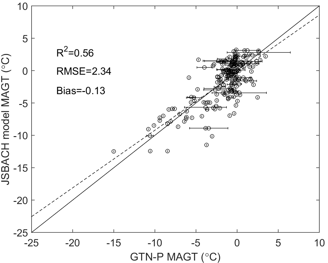
Figure 1 Evaluation of mean annual ground temperature against GTN-P borehole measurements. Model results are taken from the depth of observation for each point.

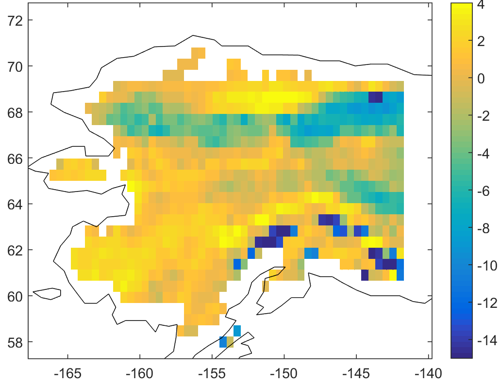
Figure 2 Difference in subsoil temperature (^∘C) between the models JSBACH and GIPL1.3 from the University of Alaska Fairbanks (1980–1989 average). JSBACH results from 38 m depth.

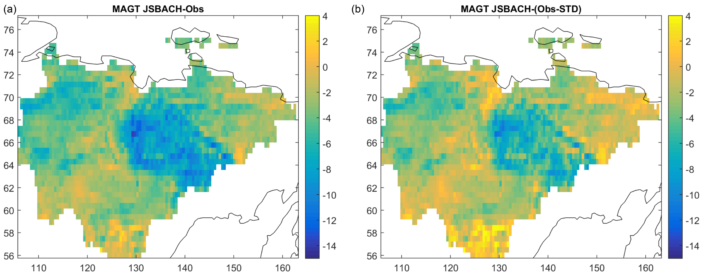
Figure 3 Difference in subsoil temperature (^∘C) between the JSBACH model (1960–1990 average) and the Geocryological Map of Yakutia (Beer et al., 2013a). JSBACH results from 38 m depth. The right-hand-side figure shows the difference to MAGT mean minus standard deviation (spatial uncertainty) from the Geocryological Map of Yakutia.

When looking at alternative estimates of spatial details of MAGT, JSBACH underestimates or overestimates MAGT by about 2 to 4 ^∘C depending on the location (Figs. 2 and 3). The JSBACH results for Alaska are compared to another model output. JSBACH overestimates MAGT in many areas in Alaska by several ^∘C, while also underestimating MAGT at the southern end of the North Slope (Fig. 2). In eastern Siberia (Yakutia), the model usually underestimates MAGT by 2 to 6 ^∘C (Fig. 3) as compared to an observation-based map (Beer et al., 2013a). However, the cold bias is largely reduced when taking the uncertainty (standard deviation) in the original geocryological map into account (Fig. 3). Then, the difference is negligible in many regions. Still, there is a very strong cold bias in the mountainous regions of eastern Siberia. When taking the map uncertainty into account (Fig. 3), the model still underestimates MAGT by about 6 to 8 ^∘C here. This bias also cannot be explained by the general warm bias of very low MAGT in the geocryological map when comparing to GTN-P observations (Beer et al., 2013a). In fact, very low snow depth model results in these areas of about 15 cm on average (data not shown) seem to be the reason for a too-low insulation of soil during a very cold winter.

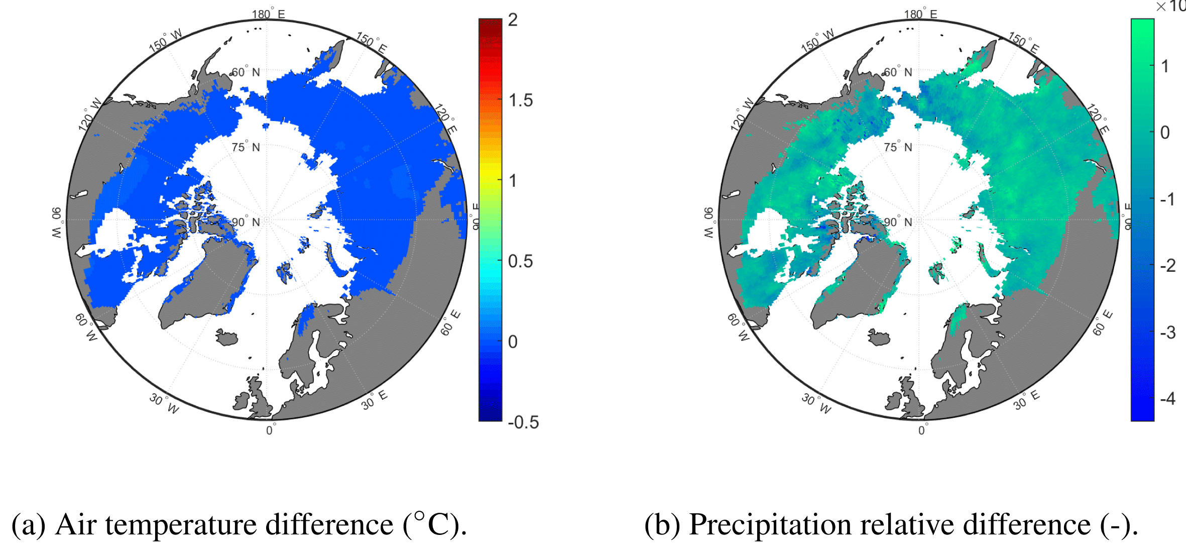
Figure 4 Comparison of 1980–2009 averages of meteorological variables (REDVAR−CNTL) or (REDVAR−CNTL) / CNTL. Air temperature colour scale adjusted to Fig. 9.

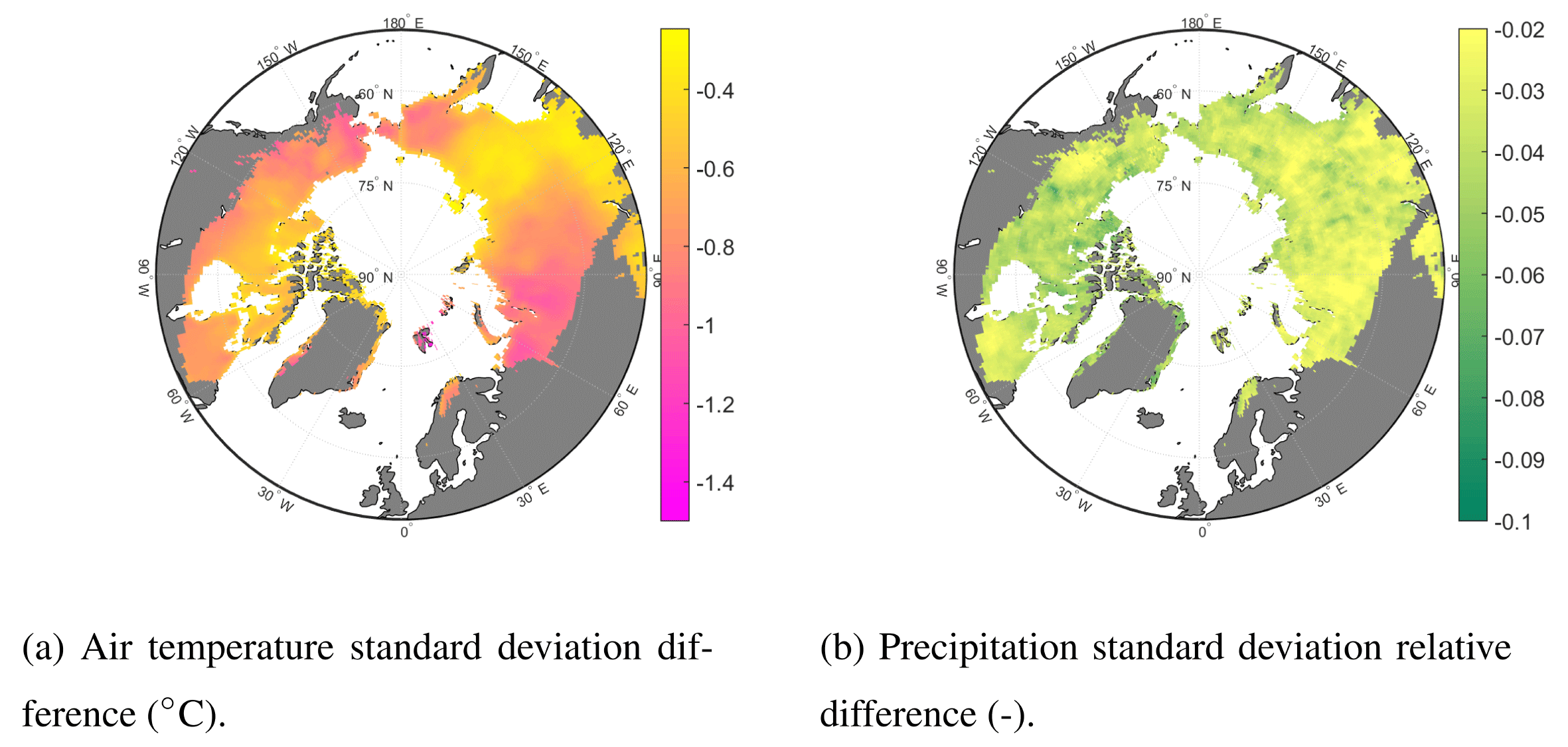
Figure 5 Comparison of 1980–2009 standard deviations of meteorological variables (REDVAR−CNTL) or (REDVAR−CNTL) / CNTL.

3.2 Climate forcing data comparison

The long-term (1980–2010) averages of air temperature differ by only 0.015 ^∘C at maximum or 0.004 % between CNTL and REDVAR in permafrost regions (Fig. 4a). Long-term precipitation averages are also similar between the datasets, with differences of −0.2 to 0.1 % (Fig. 4b).

In contrast, the difference in short-term variability of meteorological variables at daily resolution between both datasets is remarkable. Although the statistical transformation of variables has been performed at residuals to the mean seasonal cycle (Sect. 2.3), still the standard deviation of air temperature at daily resolution is usually 0.2 to 1 ^∘C lower in the REDVAR dataset than in CNTL, or 2 to 10 % (Fig. 5a). That means that temperature of warmer days have been reduced, while air temperature of colder days have been increased such that the overall mean air temperature is similar. Interestingly, the amount of variability difference between the two datasets also depends on the location. For example, smaller differences in standard deviation are visible in colder regions, such as eastern Siberia and the Canadian High Arctic. One explanation for this pattern is the higher mean seasonal cycle in continental climate, which has not been manipulated (Sect. 2.3) and which therefore dominates stronger the overall variability, which is analysed in Fig. 5a. REDVAR precipitation standard deviation is also usually 2 to 6 % lower than precipitation standard deviation of the CNTL dataset (Fig. 5b). Hence, in this artificial climate dataset, extremely heavy rainfall or snowfall is reduced, while small precipitation amounts are increased.

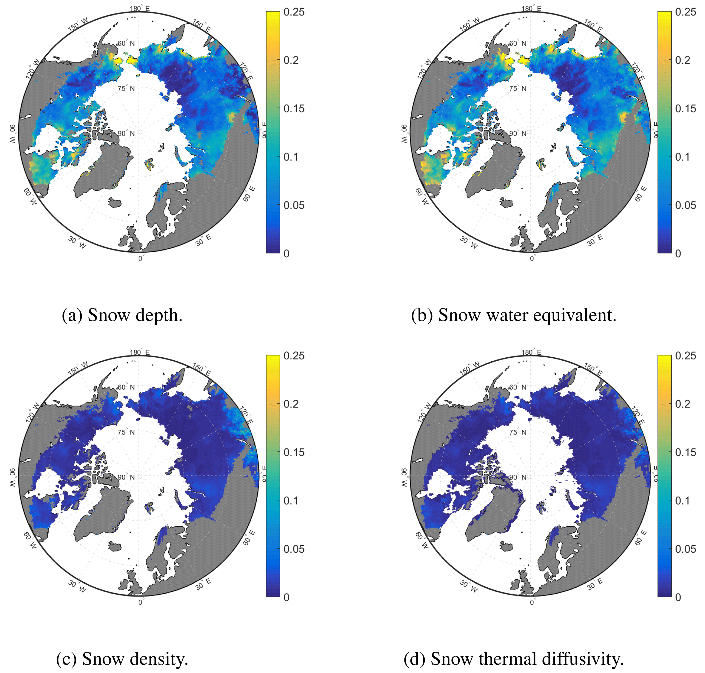
Figure 6 Comparison of mean winter (DJF) season snow properties during 1980–2009. Shown is the relative difference (REDVAR−CNTL) / CNTL expressed as a fraction (–).

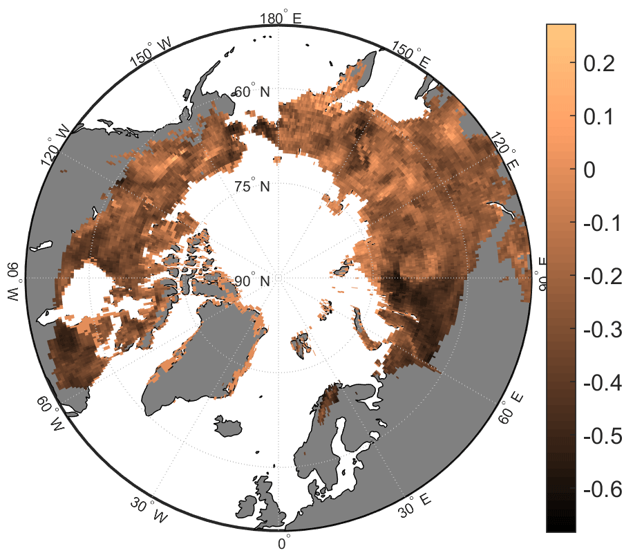
Figure 7 Autumn (SON) 1980–2009 average snowmelt relative difference. Relative difference (REDVAR−CNTL) / CNTL expressed as a fraction (–).

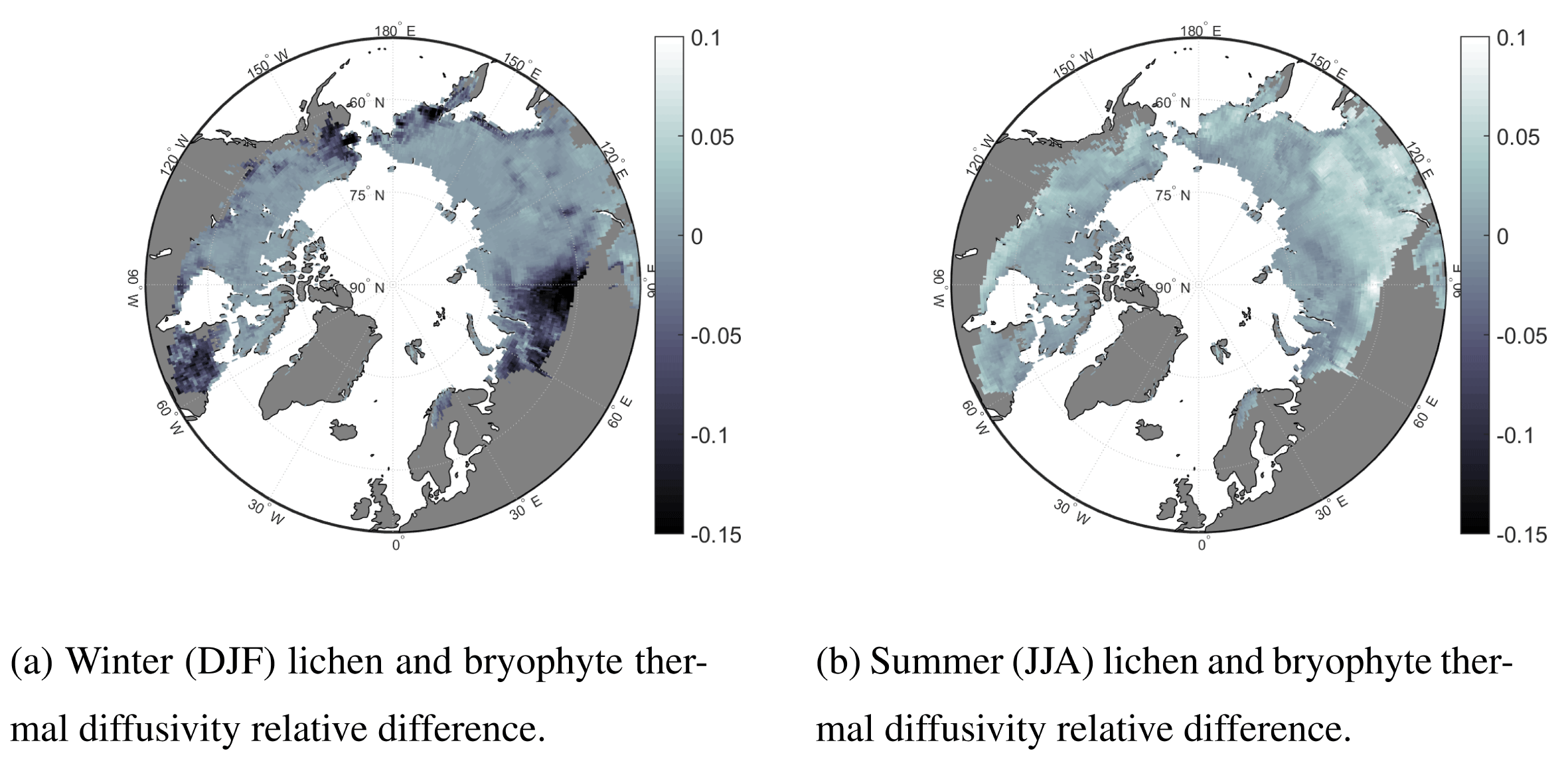
Figure 8 Comparison of lichen and bryophyte 1980–2009 average properties. Relative difference (REDVAR−CNTL) / CNTL expressed as a fraction (–).

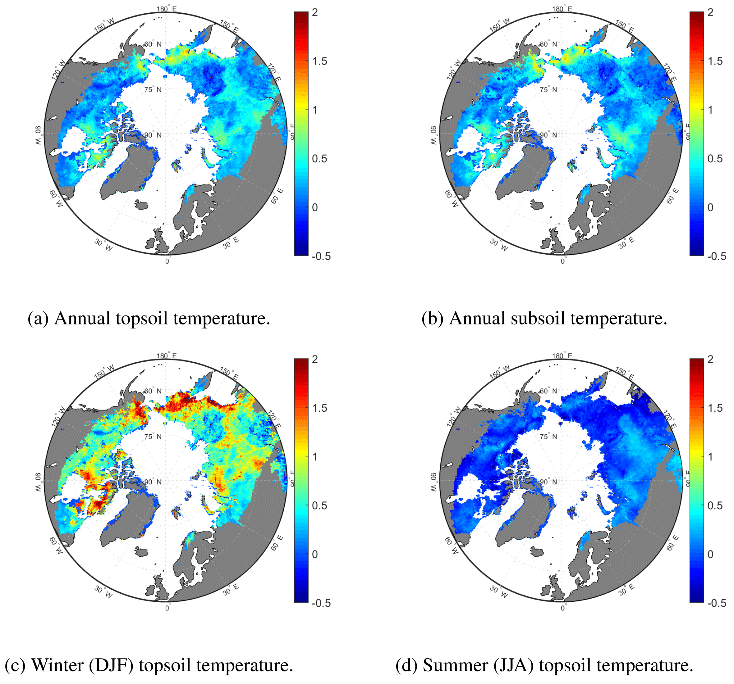
Figure 9 Comparison of 1980–2009 average soil temperature (REDVAR minus CNTL). Shown are absolute differences (^∘C). Topsoil and subsoil refer to depths of 3 cm and 38 m, respectively.

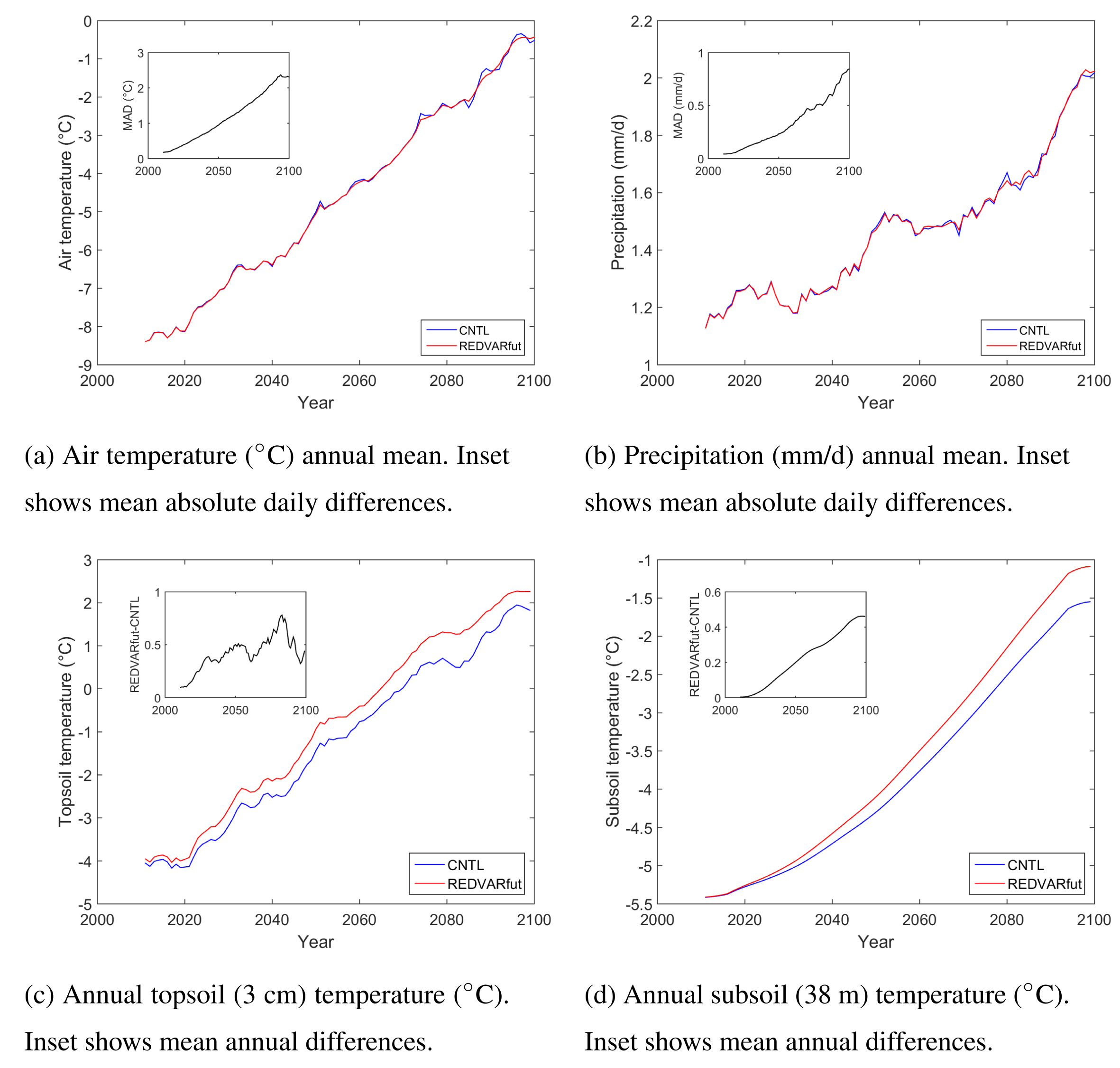
Figure 10 REDVARfut experiment results at a Canadian site (62.2^∘ N, 75.6^∘ E) during 2011–2100 showing the effects of changing climate variability on future soil temperature. Ten-year moving means are shown.

Figure 11 REDVARfut experiment results at a Siberian site (72.2^∘ N, 147^∘ E) during 2011–2100 showing the effects of changing climate variability on future soil temperature. Ten-year moving means are shown.

3.3 Climate variability effects on snow properties

Importantly, snow depth is up to 20 % higher under conditions of reduced climate variability (Fig. 6a). In fact, the snow depth difference can be explained by differences in snow water equivalents of the same magnitude (Fig. 6b). In contrast, the slightly higher snow density under reduced climate variability (Fig. 6c) is not able to explain the difference in snow depth. Snowmelt flux differences in autumn between both model experiments of 10 to 40 % (Fig. 7) demonstrate clearly that, under reduced air temperature variability during the beginning of the snow season, individual snowmelt events and hence the total snowmelt flux are reduced. Besides snow depth, the thermal diffusivity of snow controls the overall heat conduction. Figure 6d shows that, under conditions of reduced climate variability, thermal diffusivity of snow is 0.5 to 2.5 % higher in high-latitude regions.

3.4 Climate variability effects on thermal diffusivity of lichens and bryophytes

Thermal diffusivity of lichens and bryophytes differs only marginally between the REDVAR and CNTL model experiments over most of the northern high-latitude permafrost regions (Fig. 8a). In western Siberia and Quebec, winter thermal diffusivity of bryophytes and lichens is up to 12 % lower under conditions of reduced climate variability (Fig. 8a). In contrast, summer diffusivity of bryophytes and lichens is usually higher under reduced variability of meteorological variables (Fig. 8b). Under these climate conditions, it rains a little bit more often and air temperature is not extreme, resulting in more moist conditions for lichens and bryophytes, and hence higher thermal diffusivity. In tundra the difference is about 2 %, while in the boreal forest it can be up to 6 % (Fig. 8b).

3.5 Ultimate climate variability effects on soil temperature

The estimated long-term average of both topsoil and subsoil temperature differs between REDVAR and CNTL experiments (Fig. 9a and b). Soil is 0.1 to 0.8 ^∘C warmer when climate variability is reduced (Fig. 9a and b). These results and also the spatial pattern are similar between topsoil and subsoil values (Fig. 9a and b), with a slightly larger effect on topsoil temperature. Soil temperature differences are larger in winter, with values up to 1.5 ^∘C, than in summer, when differences are typically 0.2–0.5 ^∘C (Fig. 9c and d).

3.6 Effects of future changes of climate variability on soil temperature

In order to analyse effects of changing variability of meteorological variables into the future, the results of the respective additional future projections at two sites are displayed as time series in Figs. 10 and 11. In contrast to the continental model experiments, in these additional point simulations the variability of meteorological variables is increasingly reduced during 2011–2100 in the REDVARfut input dataset, while the historical climate until 2010 is identical (Sect. 2.3).

The bias-corrected MPI-ESM CMIP5 model output following RCP8.5 shows increasing air temperature at both locations (solid blue line in Figs. 10a and 11a). Precipitation is also increasing but not constantly (solid blue line in Figs. 10b and 11b). Meteorological forcing data of the REDVARfut dataset (red lines) show similar long-term averages to the CNTL dataset (Figs. 10a, b, and 11a, b). Hence, REDVARfut meteorological variables follow the general positive trend. However, the two time series increasingly differ in their day-to-day and week-to-week variability by design. This is shown by the mean absolute difference of daily data (cf. Eq. 5) in the insets of Fig. 10a and b as well as Fig. 11a and b.

These CNTL and REDVARfut climate datasets have been used as forcing data for JSBACH in the additional point-scale model runs. The respective soil temperature results are compared to each other in Fig. 10c and d as well as Fig. 11c and d. The increasing differences in the variability of meteorological variables under conserved long-term averages lead to an increasing difference in topsoil temperature (Figs. 10c and 11c); i.e. the overall increasing topsoil temperature due to increasing air temperature is a bit higher in the case of reduced climate variability. This effect is also visible in 38 m depth (Figs. 10d and 11d) even though short-term atmospheric data fluctuations in general should be most filtered at this soil depth.

4 Discussion

Climate model projections show increasing variability of meteorological variables and hence increasing frequency of extreme meteorological events (Seneviratne et al., 2012) along with a gradually changing climate (change of long-term mean values) (Ciais et al., 2013). Because of the non-linearity of ecosystem response functions, changing extreme-event frequency and changing variability of meteorological variables can have a higher impact on ecosystem state and function than a gradual change of mean meteorological variables (Reichstein et al., 2013; Beer et al., 2014). This study contributes to this overall question from a theoretical point of view with LSM experiments for which artificially manipulated climate forcing datasets have been employed. These climate datasets practically do not differ in their decadal averages (Sect. 3.2), whereas they do show a substantial difference in the short-term (daily) variability (Sect. 3.2). Therefore, differences in simulated state variables and fluxes over 30-year periods (soil temperature in this case) will be only due to differences in temporal variability of meteorological variables. This study addresses particularly the question about the effect of climate variability on soil temperature in northern high-latitude regions. The CNTL experiment shows higher climate variability than the artificial experimental REDVAR dataset (Sects. 2.3 and 3.2), and respective model result differences between experiments using the manipulated climate REDVAR and the CNTL dataset are shown in Sect. 3. Methodologically, it is important to artificially design a climate dataset with reduced temporal variability because otherwise there is a high risk for producing a physically unrealistic climate conditions. However, for interpreting the results in terms of future ecosystem responses to increasing climate variability (Seneviratne et al., 2012), the results of the CNTL model run are compared against the results of the REDVAR model run in this discussion section (CNTL–REDVAR).

In contrast to the climate forcing data, the long-term average of both topsoil and subsoil temperature differs between REDVAR and CNTL experiments (Fig. 9a and b). The same is true for respective future projections (Figs. 10 and 11). In fact, under conditions of higher variability of meteorological variables and higher frequency of extreme events (CNTL vs. REDVAR experiments), soil will be cooler (Figs. 9c, d; 10; and 11) if all other environmental factors are similar. That means that the projected increase in future variability of meteorological variables (Seneviratne et al., 2012) has the potential to dampen soil warming occurring as a function of increasing mean air temperature. To further understand the underlying processes, individual effects of climate variability on snow and near-surface vegetation properties are discussed in the following paragraphs.

For land–atmosphere heat conduction the thermal properties of snow, near-surface vegetation (e.g. bryophytes and lichens), the soil organic layer, and their spatial extent and heights are of major importance (Yershov, 1998; Gouttevin et al., 2012; Jafarov and Schaefer, 2016; Wang et al., 2016). Snow generally insulates the soil from changing atmospheric temperature. However, effects are smaller during the melting period in spring because the snow is wet and conductivity therefore higher, and more importantly, the soil-to-air gradient in temperature is small. The insulation effect of near-surface vegetation also differs among the seasons because of the high dependence of thermal properties on water and ice contents of lichens and bryophytes. Usually, dry lichens and bryophytes during a continental summer should insulate much more than during wet spring or autumn, or during the ice-rich wintertime.

This theoretical study shows that one major effect of higher climate variability on cold-region environments is a lower snow water equivalent (Sect. 3.3), which directly translates into lower snow depth values. The potential alternative explanation for a lower snow depth would be a higher snow density. However, the results show exactly the opposite (Fig. 6c). In addition to snow depth, snow thermal properties are also an important factor for heat conduction. However, winter snow thermal diffusivity is some percent lower under conditions of higher climate variability (CNTL–REDVAR). Therefore, the net snow-related effect of higher climate variability on soil temperature – that is, a cooler soil (Sect. 3.5) – is explained by snow depth differences alone, i.e. a lower snow depth under conditions of higher climate variability.

The reason for these snow water equivalent differences are more often circumstances of melting snow during the beginning of the snow season when day-to-day variability of air temperature is higher (Sect. 3.3). These results also point to an interesting combination of impacts of both changing variability and gradually changing mean values on ecosystem states because both changes can lead to a threshold value (melting point in this case) being passed. These impacts can be seen in Sect. 3.3 when combining temporal climate variability effects on snow water equivalent results (Fig. 6) and snowmelt flux results (Fig. 7) with longitudinal pattern of these results towards a continental climate, which can be interpreted in terms of gradual climate change when substituting space for time. Overall, these findings show that projected higher climate variability in future can lead to lower snow depth, which will reduce a soil warming in response to air warming. Future studies should clarify if these temporal variability effects of meteorological variables on snow depth are lower or higher when taking into account lateral heterogeneity of soil properties (Beer, 2016) or snow, for instance due to snow intercept by topography or vegetation.

In addition to the insulating effect of snow, lichens and bryophytes growing on the ground influence heat conduction (Porada et al., 2016a). It is interesting to note that, when climate variability is higher (CNTL conditions), bryophyte and lichen thermal diffusivity can be substantially higher in winter and lower in summer in the same region (Sect. 3.4). This fact points to an important role of near-surface vegetation: it will insulate less from air temperature during winter and insulate more during summer with increasing climate variability in future. These effects of climate variability on thermal diffusivity of lichens and bryophytes and hence soil temperature are in the same direction as snow effects (Sect. 3.3), again reducing the soil warming effect of future climate change.

Effects of climate variability on both snow and bryophyte and lichen properties are in the same direction (Sects. 3.3 and 3.4). As a result, soil will be cooler under conditions of higher climate variability (Sect. 3.5). Recent modelling studies suggest a soil temperature increase of 0.02 ^∘C per year since 1960 (McGuire et al., 2016), which translates into 2 ^∘C in 100 years. Such soil temperature increase has also been projected using the JSBACH model under the RCP4.5 scenario (Ekici, 2015), while under the strong-warming scenario RCP8.5, the soil temperature increase might be up to 6 to 8 ^∘C (Ekici, 2015). Lower soil temperature under conditions of higher climate variability in the range 0.1 to 0.8 ^∘C (Sect. 3.5) demonstrates that, under increasing variability of meteorological variables and increasing extreme events in the Arctic (Seneviratne et al., 2012), the effect of gradual air temperature increase on soil temperature and hence active-layer thickness will be dampened. Such dampening of future soil warming will also reduce the otherwise positive biogeochemical feedback to climate (Zimov et al., 2006; Beer, 2008; Heimann and Reichstein, 2008). Our results are conservative here because the 99 percentiles of air temperature and precipitation from the artificial dataset (REDVAR) differ by only 1–4 ^∘C (temperature) and 1–10 % (precipitation). These values are at the lower end of the range of climate model projections for the Arctic region until 2100 (Seneviratne et al., 2012).

The presented effects of short-term variability of meteorological variables on ecosystem states and functions, such as soil temperature, are also important from a methodological point of view. To study the effects of environmental change on ecosystems, LSMs are usually forced by historical and reanalysis climate data for the past and present periods, and by future climate results from Earth system models. Since ESM results usually show biases, the ESM outputs cannot be used directly to drive the LSM offline model runs but first need to be bias-corrected (Hempel et al., 2013). The results of the presented REDVAR and REDVARfut experiments demonstrate that such bias-correction methods should account for the projected change in short-term (daily) variability in addition to general trends.

Soil temperature is projected to arrive at values around the freezing point in 38 cm depth over the major part of the current permafrost area (Schaphoff et al., 2013). Therefore, differences of soil temperature of 0.1 to 0.8 ^∘C due to changing climate variability would have an effect on active-layer thickness and permafrost extent, too. It would be interesting to generate an additional artificial REDVARfut dataset with pan-Arctic cover and investigate in detail the impacts of climate variability on active-layer thickness and permafrost extent at the end of the century in a future project

Our findings have three major implications for future permafrost science:

1. New, highly controlled laboratory and field experiments are required in order to confirm modelling results about climate variability effects on permafrost soil temperature.

2. Future developments of land surface models should include dynamic models of snow, and lichens and bryophytes.

3. Statistical methods need to be developed such that future forcing data for climate change impact studies can be prepared in a way that a potential change in short-term variability and frequency of extreme events is preserved.

5 Conclusions

Artificial model experiments have been used in order to quantify the impact of the variability of meteorological variables on the long-term mean of mean annual ground temperature in permafrost-affected terrestrial ecosystems. In future, the soil temperature response to increasing climate variability and extreme-event frequency (soil cooling) will be opposite to the response of soil temperature to gradually increasing air temperature (soil warming). Is has been shown that snow and near-surface vegetation dynamics are the underlying mechanisms for this. Therefore, dynamics of snow and lichen and bryophyte functions need to be represented in Earth system models for validly projecting future permafrost soil states and land–atmosphere interactions, and hence future climate. Our findings also point to the need to represent changes in short-term variability of meteorological variables in bias-corrected climate data of future periods.