the Creative Commons Attribution 4.0 License.
the Creative Commons Attribution 4.0 License.
 | 06 Feb 2018
Tidal influences on a future evolution of the Filchner–Ronne Ice Shelf cavity in the Weddell Sea, Antarctica
Rachael D. Mueller
Tore Hattermann
Susan L. Howard
Laurie Padman
Recent modeling studies of ocean circulation in the southern Weddell Sea, Antarctica, project an increase over this century of ocean heat into the cavity beneath Filchner–Ronne Ice Shelf (FRIS). This increase in ocean heat would lead to more basal melting and a modification of the FRIS ice draft. The corresponding change in cavity shape will affect advective pathways and the spatial distribution of tidal currents, which play important roles in basal melting under FRIS. These feedbacks between heat flux, basal melting, and tides will affect the evolution of FRIS under the influence of a changing climate. We explore these feedbacks with a three-dimensional ocean model of the southern Weddell Sea that is forced by thermodynamic exchange beneath the ice shelf and tides along the open boundaries. Our results show regionally dependent feedbacks that, in some areas, substantially modify the melt rates near the grounding lines of buttressed ice streams that flow into FRIS. These feedbacks are introduced by variations in meltwater production as well as the circulation of this meltwater within the FRIS cavity; they are influenced locally by sensitivity of tidal currents to water column thickness (wct) and non-locally by changes in circulation pathways that transport an integrated history of mixing and meltwater entrainment along flow paths. Our results highlight the importance of including explicit tidal forcing in models of future mass loss from FRIS and from the adjacent grounded ice sheet as individual ice-stream grounding zones experience different responses to warming of the ocean inflow.
- Article
(9732 KB) - Full-text XML
-
Supplement
(93 KB) - BibTeX
- EndNote


The dominant terms in the mass balance of the grounded portion of the Antarctic Ice Sheet are gains from snowfall and losses by gravity-driven flow of ice into the ocean. Around the ocean margins, the ice sheet thins sufficiently to float, forming ice shelves. Continuous gravity measurements from the GRACE satellite during 2002–2015 (Harig and Simons, 2015; Groh and Horwath, 2016) show that the non-floating, grounded, ice mass is decreasing. This decrease in mass loss is attributed to recent acceleration of ice shelf thinning (Pritchard et al., 2012; Rignot et al., 2013). Most of this net mass loss is occurring in the Amundsen Sea sector (Sutterley et al., 2014), predominantly in glaciers flowing into Pine Island Bay (Mouginot et al., 2014; Khazendar et al., 2016), and is observed as glacier acceleration, ice-sheet thinning, and grounding-line retreat. Losses in this sector are correlated with observed thinning of the ice shelves (Pritchard et al., 2009, 2012; Paolo et al., 2015), consistent with a reduction in back-stress (buttressing) that impedes the seaward flow of the grounded ice (e.g., Scambos et al., 2004; Dupont and Alley, 2005; Rignot et al., 2014; Joughin et al., 2014). These studies demonstrate a need for improving predictions of how the extent and thickness of ice shelves will evolve as climate changes.
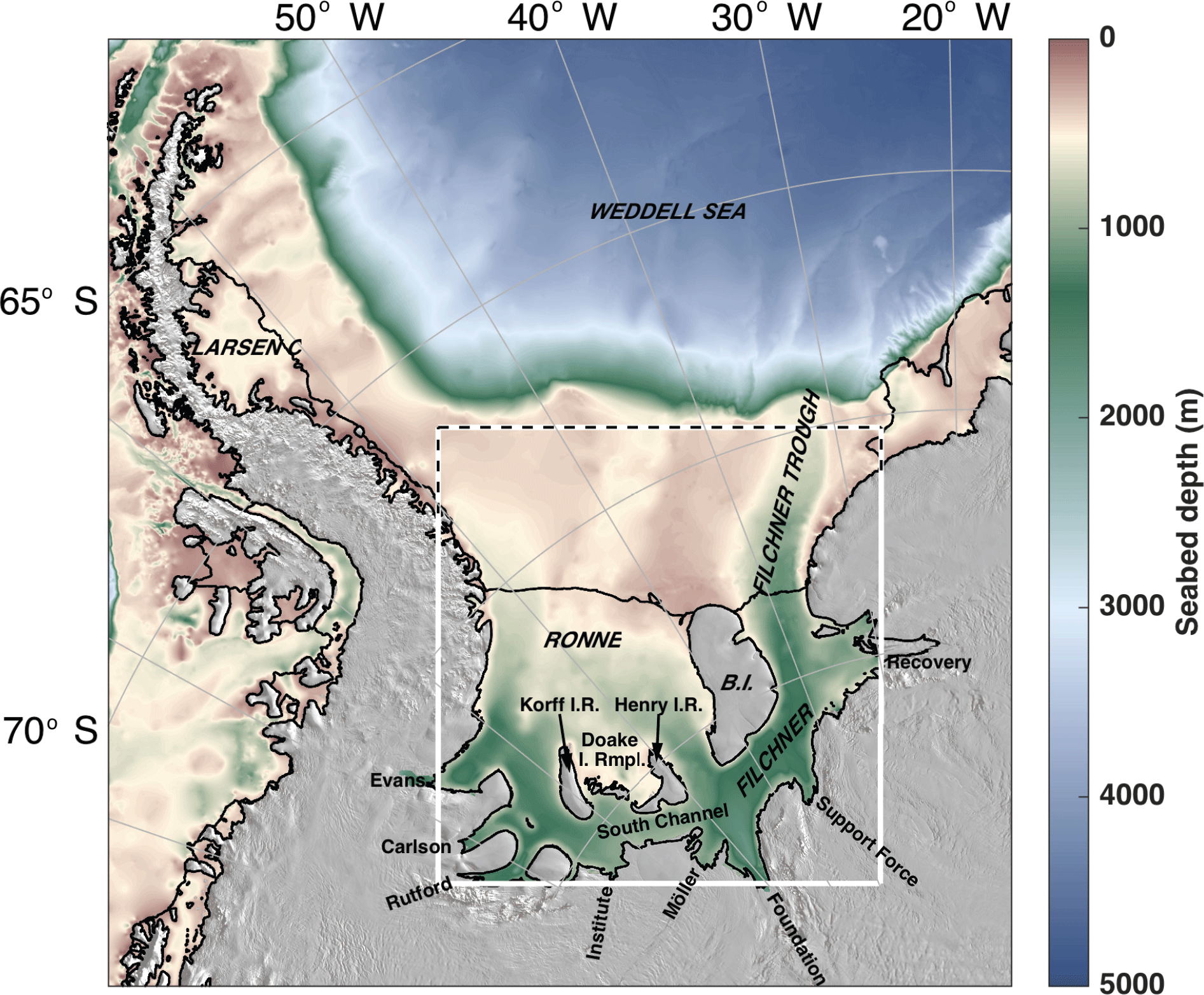
Figure 1The Weddell Sea region of study with the model domain outlined by the white box. Dashed black lines highlight the open boundaries. The labels on land indicate the names of the tributary glaciers used for regional analyses in this study. Black lines over seabed indicate the extent of the ice shelf while black lines around the grey mask indicate the ice sheet grounding line and/or transition between ocean and land.
The mass budget for an ice shelf is the sum of mass gains from both snow accumulation and advection of ice across the grounding line, combined with mass losses from iceberg calving, basal melting, surface runoff, and sublimation. Calving and melting each contribute roughly half of the total Antarctic Ice Sheet mass loss (Rignot et al., 2013; Depoorter et al., 2013). Surface runoff and sublimation are insignificant for most Antarctic ice shelves. The ice shelves that are currently experiencing the most rapid thinning are in the Amundsen and Bellingshausen seas where melting exceeds calving due to the influence of relatively warm Circumpolar Deep Water (CDW) on the heat content within these ice shelf cavities (Jenkins and Jacobs, 2008; Padman et al., 2012; Jenkins et al., 2010b; Jacobs et al., 2013; Schmidtko et al., 2014). The large ice shelves in other sectors that are not directly influenced by CDW inflows are closer to steady state, suggesting that the transport of ocean heat under these ice shelves has not changed significantly over the observational record.
We focus here on one of these large ice shelves, Filchner–Ronne Ice Shelf (FRIS), in the southern Weddell Sea (Fig. 1). FRIS accounts for 30 % (∼ 430 000 km2) of the total area of Antarctic ice shelves and only 10 % of the total ice shelf mass loss. For comparison, Pine Island Glacier accounts for 0.4 % of the total area of Antarctic ice shelves and 7 % of the net ice shelf mass loss (Rignot et al., 2013). Models suggest that the disproportionately small melt contribution from FRIS to ice shelf mass loss may change in the coming century in response to a future climate scenario forcing a large and persistent increase in ocean temperatures beneath FRIS (Hellmer et al., 2012; Timmermann and Hellmer, 2013). In the modern state, most of the water entering the ocean cavity under Filchner Ice Shelf (FIS) and Ronne Ice Shelf (RIS) is derived from high-salinity shelf water with a temperature close to the surface freezing point of −1.9 ∘C (Nicholls et al., 2009). Traces of modified warm deep water with temperature up to about −1.4 ∘C are found in the Filchner Trough near the FIS ice front (Darelius et al., 2016) and at the RIS front (Foldvik et al., 2001) with evidence that this water may influence sub-ice shelf melt in the outer 100 km of the ice shelf (Darelius et al., 2016). Hellmer et al. (2012) show that future changes in circulation may allow for more inflow of warm deep water into the ice shelf cavity, displacing the high-salinity shelf water beneath FRIS by the end of the 21st century and increasing basal melt rates an order of magnitude higher than at present. In this warm state, the associated rapid thinning of the ice shelf would reduce the buttressing of the large marine-based grounded ice sheet surrounding FRIS (Ross et al., 2012), significantly accelerating future sea level rise (Mengel et al., 2016). Furthermore, simulations by Hellmer et al. (2017) show that the increased meltwater production will sustain the warm inflow even if atmospheric conditions were reversed to a colder state, suggesting the existence of an irreversible tipping point once melting increases past a certain threshold.
These estimates of increased melt, however, assume that cavity geometry does not change in a way that alters the access of ocean heat to the FRIS base. Studies of Larsen C Ice Shelf (Mueller et al., 2012) and Pine Island Glacier ice shelf (Schodlok et al., 2012) showed that changes to the ice shelf cavity shape can significantly alter the spatial pattern of basal melt rate, particularly in regions where tidal currents contribute substantially to the total turbulent kinetic energy near the ice base. Tides were not explicitly included in the forcing for the Hellmer et al. (2012) study; however, tidal currents often play a critical role in setting the pattern and magnitude of basal melt rates under cold water ice shelves (MacAyeal, 1984; Padman et al., 2018) including FRIS (Makinson et al., 2011), which leads us to hypothesize that tides would influence changes in meltwater production from a warming ocean.
We explore this hypothesis using a suite of numerical model simulations that incorporate variations in tide forcing, initial temperature, and cavity geometry together with thermohaline interactions at the interface between the ocean and ice shelf. We then use these models to describe how feedbacks between ice shelf thinning and predicted tidal currents in the ice shelf cavity influence the evolution of a tide-dominated ice shelf environment under the condition of increased influx of ocean heat. Lastly, we consider the role of tides on basal mass loss near the grounding lines of each of the major ice streams supplying ice to FRIS as a guide to how individual ice-stream grounding zones might respond to the projected increase in ocean heat flux to the FRIS cavity.
2.1 Model overview and thermodynamic parameterization
Our simulations were carried out with a version of the Regional Ocean Modeling System (ROMS 3.6; Shchepetkin and McWilliams, 2009) that has been modified to include pressure, friction, and surface fluxes of heat and salt at the ice shelf base (Dinniman et al., 2007, 2011; McPhee et al., 2008; Mueller et al., 2012). ROMS is a hydrostatic, 3-D primitive equation model with a terrain-following (σ-level) coordinate system and Arakawa-C staggered grid. Our model domain (Fig. 1) covers a portion of the southern Weddell Sea, Antarctica, including FRIS. The grid spacing is 5 km with N = 24 vertical levels. A full description of model parameter choices and processing options is given in the Supplement.
Two model geometries were used in our set of simulations, one representing the modern state (standard geometry) and the other representing a possible future state (modified geometry). Model geometry consists of a land mask (including grounded ice sheet), seabed bathymetry (h), and ice draft (zice). These grids are described in Sect. 2.2.
Our simulations were initialized with a homogeneous, stationary ocean that has a potential temperature of either ∘C (cold case) or ∘C (warm case). Initial salinity was set as Sinit= 34.65 for all cases. Model hydrography was restored to θinit and Sinit at the boundaries using a mixed radiation and nudging condition (Marchesiello et al., 2001) with a 20-day timescale. Values of θinit and Sinit for the standard geometry cold case were chosen to approximate the primary water mass entering the ice shelf cavity at present (Foldvik et al., 2001; Nicholls et al., 2001, 2009). The consequences to FRIS cavity circulation in choosing a uniform θinit and Sinit are discussed in Sect. 4. The warm case represents a moderate ocean warming scenario with an increase of 0.5 ∘C in the temperature of water entering the FRIS cavity. This change is much smaller than the 2 ∘C temperature increase in the inflowing water by the end of this century predicted by Hellmer et al. (2012) but was chosen to investigate whether initial feedbacks due to melt-induced changes in cavity shape from initial warming might be positive or negative. Our idealized simulations do not include wind forcing, frazil ice, or sea-ice formation.
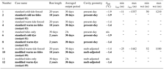
Table 1An overview of the 12 model runs presented in this paper and the case name that is used to reference them. The three runs that were used as the spin-up solutions are referenced by their number in “restart” runs (displayed in bold font) as restart #1, #3, and #9. The runs that include passive dye tracers are flagged as “dye” runs. All run intervals provide steady state solutions as determined by the transient solutions of shelf-averaged basal melt. n/a indicates where initial temperature is not applicable.
Circulation develops through buoyancy forcing caused by thermodynamic exchange at the base of the ice shelves and, for tide-forced cases, by boundary conditions of tidal depth-integrated velocity and sea surface height. The thermodynamically driven component of the circulation was introduced by scalar fluxes at the ice–ocean interface beneath FRIS. These fluxes are based on a simplified version of the three-equation parameterization (Hellmer and Olbers, 1989; Holland and Jenkins, 1999) that includes the assumption that the heat flux through the ice shelf is negligible:
In Eq. (1), the surface heat flux ( is determined by the combined effect of thermal forcing and turbulent heat exchange. The thermal forcing is represented as , where Tb is the temperature at the ice–ocean interface and To is the temperature of the ocean mixed layer under the ice base. The value of Tb is assumed to be the freezing point temperature, Tf, and depends on the salinity at the ice–ocean interface, Sb, as well as the ice draft, zice < 0 (Foldvik and Kvinge, 1974; Dinniman et al., 2007). For To, we follow a common approach of using the temperature of the surface σ layer in place of mixed layer values, with the thickness of the surface σ layer beneath the ice shelf cavity in our standard grid ranging from 2–24 m and with 72 % of points between 5 and 15 m. The turbulent heat exchange at the ice–ocean interface is represented by a thermal transfer coefficient, αh, scaled by a friction velocity, u∗. This turbulent heat exchange is then adjusted by a meltwater advection term, m, that corrects the scalar fluxes for a computational drift that is introduced as an artifact of assumptions made in the numerical representation of the ice shelf as a material boundary (Jenkins et al., 2001). We define where Sb < 5 and m= 0 elsewhere. The friction velocity is calculated from the surface quadratic stress of the upper sigma level as , where is a constant drag coefficient and is the magnitude of the surface-layer current. The potential density of seawater, , is evaluated for the uppermost layer, with the heat capacity of the ocean, cpo, assumed constant at 3985 J kg−1 ∘C−1. ΔS is the salinity equivalent to ΔT and is defined as , with Sb solved by a quadratic formula combining Eqs. (1)–(3), without the meltwater advection term (m), and with So representing the salinity of the surface σ layer.
These heat and salt fluxes ( depend on scalar transfer coefficients (αh, αs) that are proportional to each other by a double diffusive parameter, (McPhee et al., 2008). Chapter 2 in Mueller (2014) provides a more detailed explanation of the background and motivation for this parameterization. Here, we used scalar transfer coefficients based on observations of the RIS sub-ice shelf cavity (Jenkins et al., 2010a), with and R= 35.5. The meltwater-equivalent melt rate term is derived by scaling the heat flux, , by latent heat, J kg−1, and the density of ice, ρi=918 kg m−3, such that
Melting ice is indicated by wb > 0 and represents the thickness of freshwater added to the ocean surface, per second. These equations highlight that basal melting is driven by ocean heat and motion, with the latter being influenced by thermohaline circulation and tides.
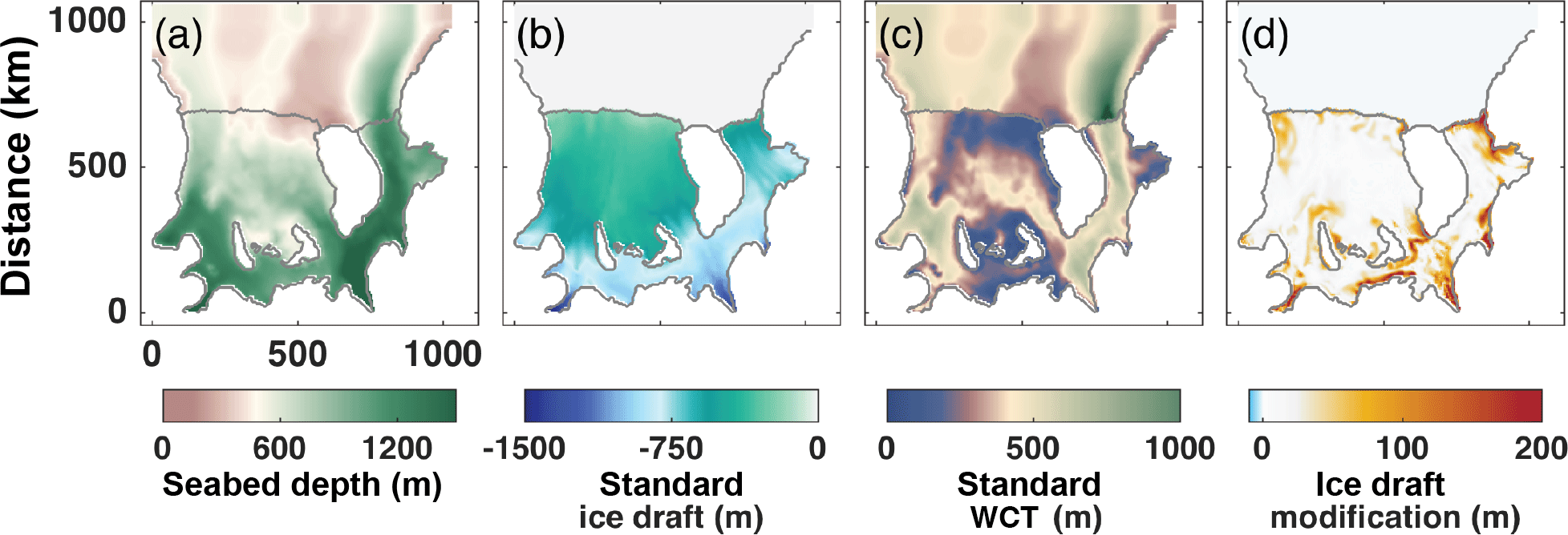
Figure 2Bathymetry (h) and ice draft (zice) for the standard and modified geometries: (a) h for both the standard and modified cases; (b) zice for the standard case; (c) water column thickness (wct) for the standard case; (d) difference between standard zice and modified zice, where difference > 0 indicates regions of melting and a corresponding decrease in zice in the modified geometry when compared to the standard geometry.
A set of 12 model simulations was performed and is summarized in Table 1. A detailed description of the different simulations is given in Sect. 2.3. Each case involves a combination of standard or modified geometry, cold or warm ocean, and tidal forcing switched off or on. For tide-forced simulations, tide heights and barotropic currents were specified along the domain's open-ocean boundaries (see Fig. 1). The tidal boundary conditions were obtained for the four most energetic tidal constituents (K1, O1, M2, and S2) from the CATS2008 barotropic inverse tide model, an updated version of the circum-Antarctic model described by Padman et al. (2002). These four constituents account for 94 % of the total tidal kinetic energy for this region, based on CATS2008 estimates. Flather (1976) boundary conditions were used for the barotropic velocity with free surface conditions following Chapman (1985). Radiation conditions for baroclinic velocities were applied following Raymond and Kuo (1984). Tracer equations were radiated across the open boundaries (Marchesiello et al., 2001) and nudged to initial conditions over a 20-day timescale.
2.2 Geometries
The grid of seabed bathymetry (h) over the entire domain (Fig. 2a) was derived from the RTOPO-1 gridded dataset (Timmerman et al., 2010). The ice shelf is represented by a non-evolving, although freely floating, surface boundary based on an ice draft (zice, Fig. 2b) that was also derived from RTOPO-1. The land mask was adjusted around the ice rises and rumples in the southern RIS to follow the grounding line provided by Moholdt et al. (2014). Values of h and zice in regions of the ice sheet that are grounded in the RTOPO-1 mask but floating (i.e., ice shelf) in the mask obtained from the Moholdt et al. (2014) data were computed by linear interpolation and a nearest-neighbor extrapolation to ice shelf points in the original RTOPO-1 grids.
The ice draft and bathymetry were each smoothed to minimize errors in the baroclinic pressure gradient that arises with the terrain-following coordinate system used in ROMS (Beckmann and Haidvogel, 1993; Haney, 1991). The two parameters used to quantify smoothing are the Beckmann and Haidvogel number, (Beckmann and Haidvogel, 1993), and the Haney number, (Haney, 1991), where , the surface σ layer, and e and e′ represent two horizontally adjacent grid cells. Together, these parameters establish that the surface (ice) and bottom bathymetry slopes are sufficiently small to reduce or eliminate spurious flows due to a horizontal pressure gradient and ensure hydrostatic consistency throughout the water column at adjacent horizontal grid nodes. Our Beckman and Haidvogel number, rx0, is less than 0.045 along both surface and bottom topographies, and our Haney number, rx1, is less than 10 in both surface and bottom levels except for some areas along the ice shelf front, where rx1 is larger and reaches a maximum value of 17.
Our maximum values of rx1 are larger than typically recommended for ROMS. To test whether large values lead to significant circulation from resulting errors in the baroclinic pressure gradient, we ran unforced models for each of the standard and modified grids. We initialized these models with horizontally uniform temperature and salinity fields, using an extreme density profile in order to get an upper bound on the grid errors. We chose a profile from a location just north of the eastern side of Berkner Island. The T and S profiles in this region yielded a relatively strong pycnocline with potential density changing from 1027.67 to 1027.77 kg m−3 between 0 and 400 m, a depth range where the change in ice draft along the ice shelf front is most likely to cause spurious flows. This profile was extrapolated in depth and horizontally to yield the uniformly stratified test hydrography. The resulting velocities in these unforced runs are representative of maximum grid errors that may occur in the full simulations. We quantified grid error by comparing the currents generated by these horizontally uniform, stratified, unforced model runs to the 30-day averaged current speeds in the standard warm tide-forced and modified warm tide-forced cases. The maximum fractional error in our velocity fields is 10 % for the standard grid and 5 % for the modified grid. Large errors were limited to a very small region north and northwest of Berkner Island; the relative error over most of the domain is negligible.
In the smoothed standard geometry, the ice draft beneath FRIS ranges from 1537 m at the deepest part of the grounding line to 11 m at the shallowest point of the ice shelf front. Small values of ice draft near the ice front are unrealistic but are a consequence of necessary smoothing in models that use terrain-following vertical coordinates. The region of thinned ice shelf represented by these small values is a narrow band along the ice front (Fig. 2b and c). The water column thickness, wct , ranges from 50 m (a specified minimum value, chosen for numerical stability) to 1111 m under FRIS. In the open ocean, wct =h and has a maximum value of 1211 m in the Filchner Trough.
Using this standard geometry, we conducted simulations for both the cold and warm cases described in Sect. 2.1, with and without tides. The modified geometry was then created from the output of the two 20-year tide-forced simulations of the standard cold and standard warm cases (see Sect. 2.3.2). In creating this grid, we assumed that RIS and FIS are both in steady state under present-day conditions (Rignot et al., 2013; Depoorter et al., 2013; Moholdt et al., 2014) represented by our standard cold case and that the most accurate simulations of basal melting will be those with tidal forcing included (Makinson et al., 2011). Steady state requires that mass input from lateral ice transport across the grounding line plus snowfall onto the ice shelf is balanced by basal melting and iceberg calving that maintains a constant ice-front position. The difference in local melt between the standard warm and standard cold cases, neglecting any ice dynamical feedbacks, would then be equivalent to the rate of change in thickness of the ice shelf, provided the change in melt rate is not offset by changes in mass inputs to the ice shelf.
We applied the melt rate imbalance for a period of 50 years to provide a sufficiently large change in zice to significantly alter the general circulation and tidal currents in the cavity. The resulting modified geometry thins zice by an average across the ice shelf of 30 m and a median of 14 m. The ice shelf thickens in the freezing (mid-shelf) regions by a maximum of 14 m and thins in the melt regions by a maximum of 453 m, although about 99 % of all thinning values are less than 200 m (Fig. 2c and d). The combined area where the ice shelf thickens is only 0.1 % of the total ice shelf area and is characterized by an average increase of 5 m. The modified-case bathymetry is the same as the standard case bathymetry, so these changes in zice cause an equal magnitude change in wct. We chose to only run the modified geometry as a warm case because it is designed to represent the FRIS cavity under warm conditions, with and without the influence of tidal forcing along the open boundaries.
2.3 Model simulations
Three types of simulations were run: (1) tide resolving with time-averaged output every 2 h and no thermodynamic exchange, (2) simulations with ice–ocean thermodynamics, with and without tide forcing, and (3) passive dye tracer simulations to explore circulation patterns. These runs are more fully described in the following sections.
2.3.1 Tide-resolving simulations with no thermodynamic exchange
We performed two 40-day simulations with 2 h averaged output, one with standard geometry and the other with modified geometry, to predict tidal current speeds. These simulations (tides-only cases) did not include thermodynamic interactions at the ice–ocean boundary, so the ocean remained unstratified at its initial homogeneous state. Absent stratification, the resulting currents are barotropic in nature, although some depth dependence arises from the friction at the seabed and ice base (see, e.g., Makinson et al., 2006).
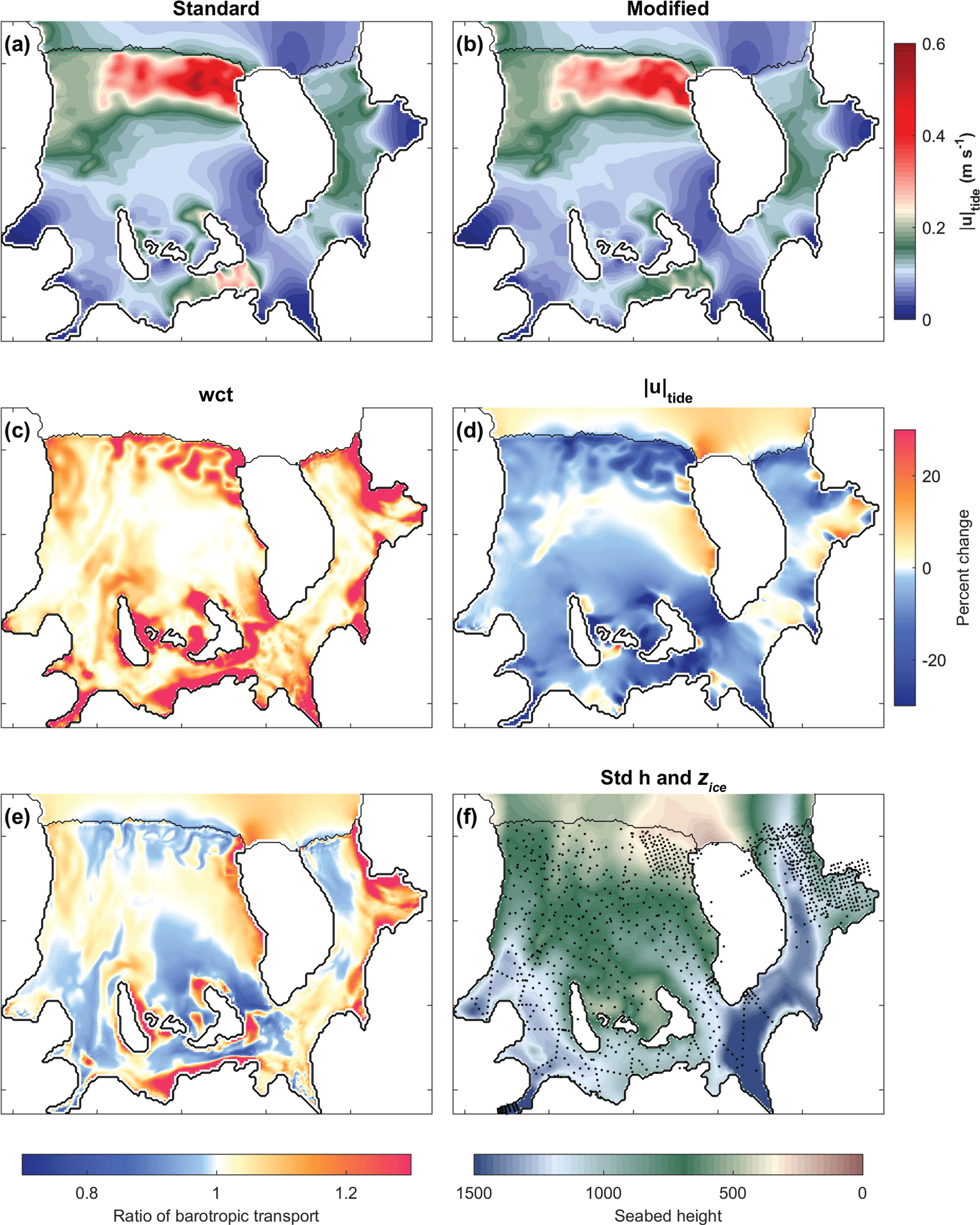
Figure 3(a) Barotropic current (, Eq. 5) for the standard tides-only run. (b) Same as (a) but for the modified tides-only run. (c) Percent change in wct between the standard and modified cases with positive values indicating where the wct is greater in the modified geometry. (d) Change in between (a) and (b) where percent change > 0 indicates locations where the standard case is greater than the modified case . (e) Ratio of barotropic tidal transport ( shown here as modified and standard, with values > 0 showing where there is increased transport for the modified case. (f) Seabed depth (as in Fig. 2a) with existing seismic observation locations shown as black dots. Std h refers to standard case h.
The spatial characteristics of time-averaged tidal currents (Fig. 3a, b) were calculated as the time- and depth-averaged tidal current speed, , given by
where and are orthogonal components of modeled, depth-averaged current and 〈〉t represents temporal averaging over the last t= 30 days of the model run, which characterizes two cycles of the 15-day spring–neap cycles generated by the M2, S2, K1, and O1 tides. The maximum tidal speed at spring tides is, typically, about .
2.3.2 Base simulations
Six simulations, each 20–30 years long, were conducted with thermodynamic exchanges of heat and freshwater at the ocean–ice shelf interface. Output for each of these simulations is shown here as the average over the last 30 days. Three of these were run with tidal forcing – two standard geometry cases, one with ∘C (cold) and one with ∘C (warm), and one modified-geometry case with ∘C (warm). We refer to these runs as standard cold tide forced, standard warm tide forced, and modified warm tide forced (Table 1). These three simulations all reached steady state solutions by 20 years. We then used the last 30-day averaged output grids in these tide-forced solutions as initial conditions for three “restart” simulations without tidal forcing, each of which reached a new steady state over 10 model years. We refer to these runs as standard cold no tides, standard warm no tides, and modified warm no tides.
2.3.3 Passive dye tracer simulations
Three simulations were run with passive dye tracers to investigate the advection and diffusion of water from different regions. These simulations were initialized with the steady state solutions of the standard cold, standard warm, and modified warm tide-forced cases. They were run for 2 years each, with 30-day averaged output. Two types of dyes were used. (1) Passive meltwater dyes were continuously added to the model's surface sigma layer at a rate of 1×10⁴wb in six regions – the grounding zones of five tributary glaciers plus South Channel, which is the region of ice shelf south of Henry Ice Rise (Fig. 4). (2) A “bulk” dye was added to the open-ocean region shown in Fig. 4. The bulk dye was initialized at a concentration of 100 %, over the entire water column, but was not replenished after these simulations began.
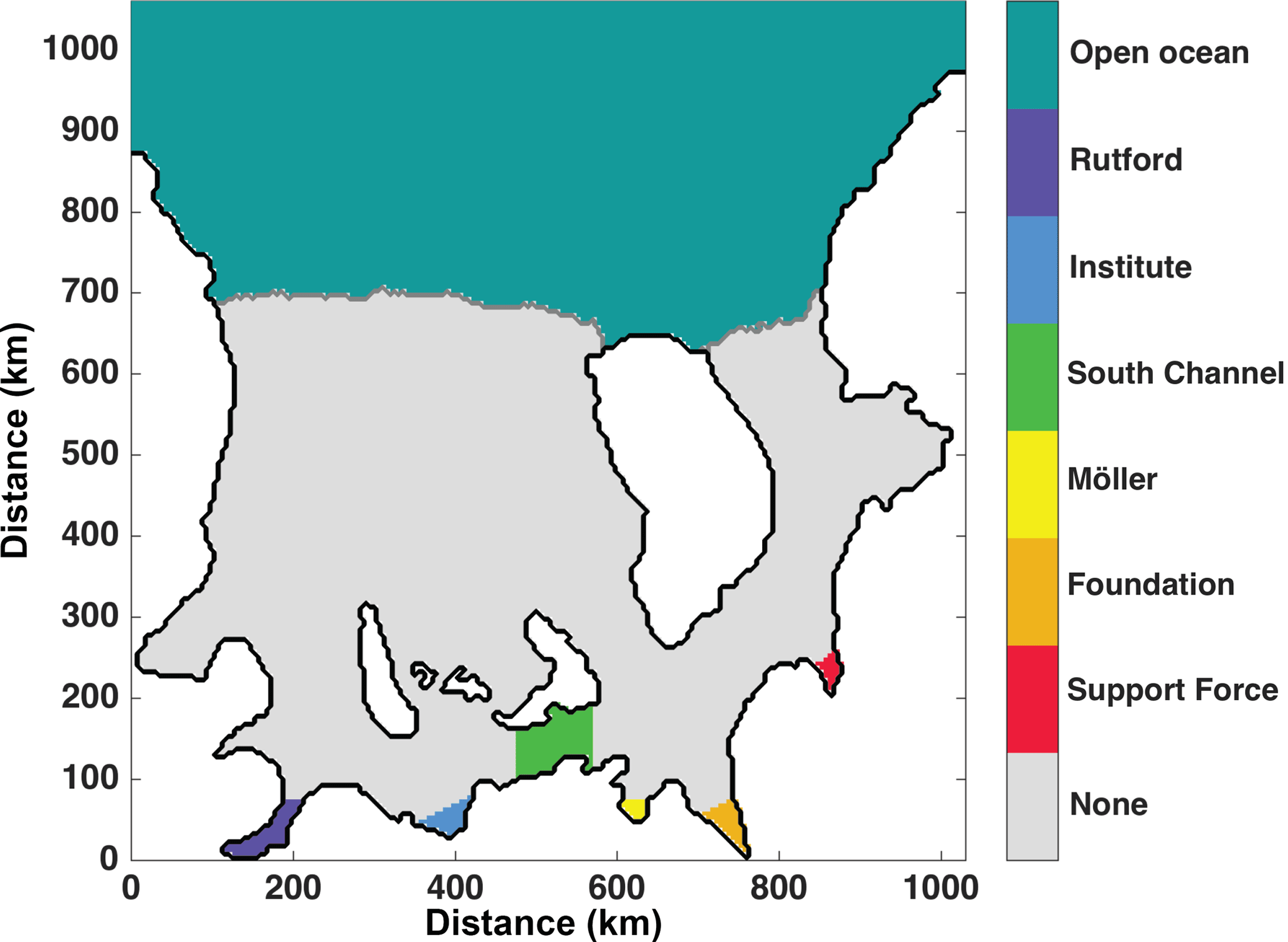
Figure 4Locations of the six, continuous, modeled meltwater dye releases and the open-ocean bulk dye explained in Sect. 2.3.3.
The main result of our study is that melt-induced changes in cavity shape introduce regional variations in tide current speeds and advection pathways that result in spatially variable feedbacks to basal melting. We explain these insights in the following subsections through analyses of tidal currents (Sect. 3.1), spatial patterns of wb (Sect. 3.2), ice-shelf-averaged wb and its sensitivity to model setup (Sect. 3.3), regionally averaged wb and its sensitivity to model setup (Sect. 3.4), and ocean circulation patterns shown by maps of the dye tracer distribution (Sect. 3.5).
3.1 Tidal currents in tide-resolving simulations
The maps of defined by Eq. (5) (Fig. 3a and b) highlight the spatial variability of tidal currents beneath FRIS. In particular, they show negligible tidal currents in the inlets of the major ice streams that feed into RIS and FIS, as well as local maxima along the northeastern RIS front and South Channel.
The maximum tidal currents along the northeastern ice shelf frontal zone of RIS are consistent with previous tide models (e.g., Robertson et al., 1998; Makinson and Nicholls, 1999). This region has a relatively small wct (Fig. 2c), so a larger tidal current here is expected. The melt-induced geometry change in the modified case (Fig. 3c) has the overall effect of increasing the water depth in this region and reducing these tidal currents (Fig. 3d).
Tidal currents in South Channel are not as strong as those in the northeastern ice shelf frontal zone, but the melt-induced change in wct and is larger than in that region (Fig. 3c and d). The melt-induced change in wct is also large along the southeastern grounding line of FIS (Fig. 3c). These changes in wct and enhance barotropic tidal transport along the southern edge of South Channel, the eastern grounding line of FIS, and along the northeast boundary of RIS with Berkner Island (Fig. 3e). These comparisons show that melt-induced ice shelf thinning generally reduces the local tidal currents (Fig. 3c, d). However, larger-scale reorganization of the barotropic tidal energy fluxes under FRIS also occurs (see, e.g., Rosier et al., 2014 and Padman et al., 2018), so simple scaling of modern tidal currents by the change in wct is not possible.
3.2 Spatial pattern of melt rates (wb) in the base simulations
We analyzed the six base simulations described in Sect. 2.3.2 to quantify the sensitivity of the spatial pattern of basal melt rates (wb) to θinit, tides, and geometry.
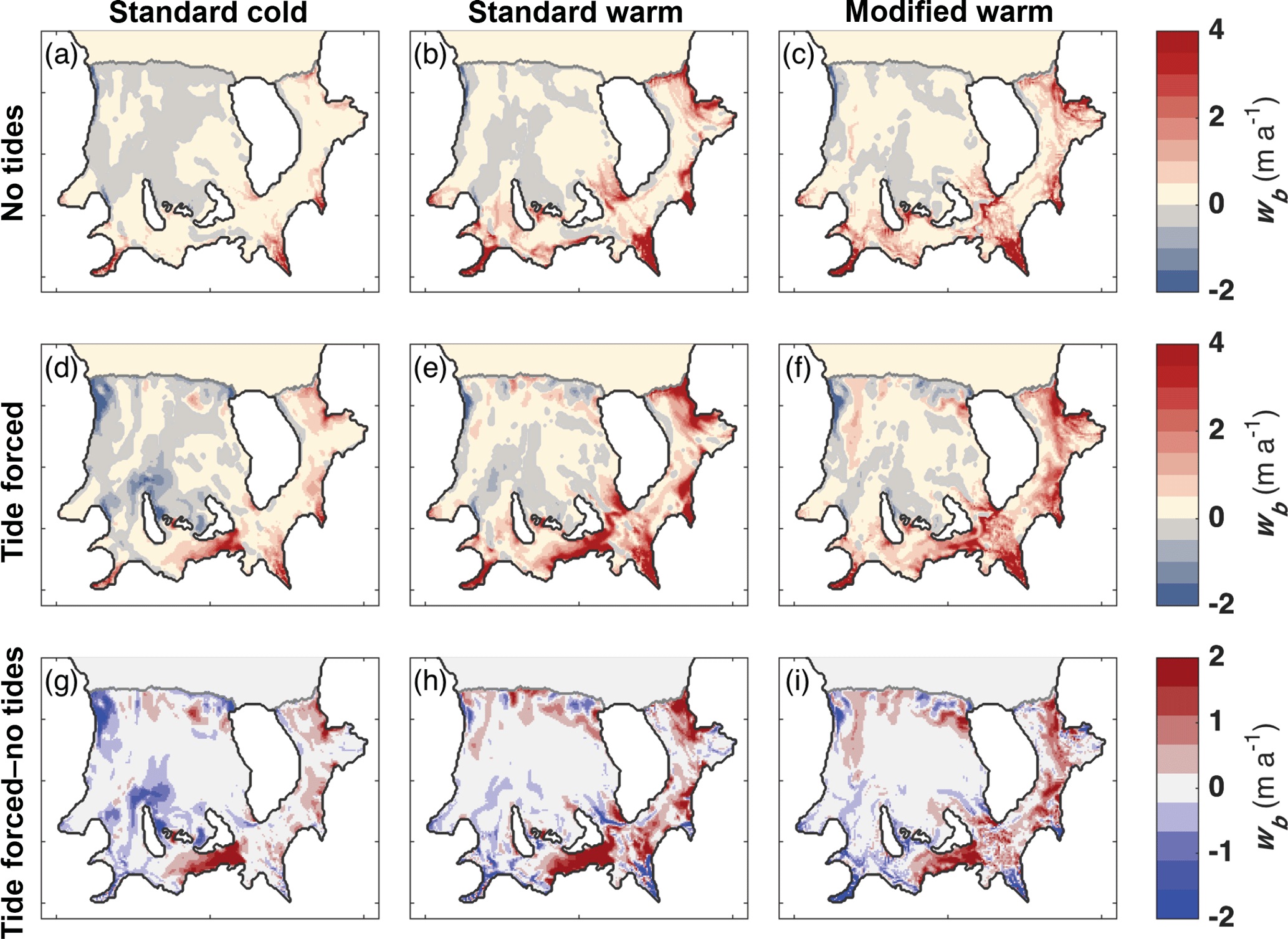
Figure 5Melt rates averaged over 1 year of steady state solutions for (top) no-tides runs, (middle) tide-forced runs, and (bottom) the difference between the tide-forced and no-tides melt solutions. Positive values in the bottom subplots show where there is more basal melting in the solutions that include tidal forcing (middle subplots). The left column (a, d, g) shows results for the standard cold case, the middle column (b, e, h) shows results for the standard warm case, and the right column (c, f, i) shows results for the modified warm case.
3.2.1 Base simulation for the no-tides cases
The pattern of wb in the standard cold no-tides case (Fig. 5a) is generally consistent with the increase in thermal forcing at the ice base due to the depression of the in situ freezing point temperature of seawater (Tf) as pressure increases. The greatest values of wb occur along the deepest grounding lines (see Fig. 2 for geometry), notably in the Support Force, Foundation, and Rutford inlets. This pattern of pressure-dependent melt fuels the ice pump mechanism that drives thermohaline circulation within the cavity and causes refreezing conditions (wb < 0) as melt water ascends to the mid-ice shelf regions, as can be seen under the central RIS and near the RIS ice front. Since our model does not include a mechanism for frazil-ice formation, these regions represent where ice would form by direct freezing onto the ice base.
The pattern of wb for the standard warm no-tides case (Fig. 5b) is generally similar to the standard cold no-tides case (Fig. 5a) but with an increase, by a factor of about 3.5, in the ice-shelf-averaged value. Changing cavity shape while imposing the same initial ocean temperature in the modified warm case (Fig. 5c) only slightly reduces melt rates (by 10 %) for the no-tides scenario (compare Fig. 5b and c).
3.2.2 Base simulation of tide-forced cases
Adding tide forcing to the standard cold case changes the magnitude and pattern of wb (compare Fig. 5a and d). Melt rates increase around the grounding line and in South Channel, (Fig. 5g). The increase in wb in South Channel, where tidal currents are relatively strong, from the standard no-tides to tide-forced cases exceeds 2 m a−1. Adding tides also increases refreezing in portions of RIS, including north of Korff Ice Rise and along the coast of the northwestern RIS, with more limited refreezing north of Henry Ice Rise. This increase in refreezing with tides can be explained by the increased production of cold, buoyant meltwater from the deeper parts of the ice shelf near the grounding line and is qualitatively consistent with the effects of adding tides reported by Makinson et al. (2011).
In the standard warm case, wb also increases around the deep grounding lines when tides are added (compare Fig. 5b and e). In this case, however, this increased melt does not enhance mid-shelf basal freeze conditions as much as in the standard cold case. Consequently, the increase in refreezing under RIS is less pronounced than for the standard cold tide-forced case (compare Fig. 5e and d). There are two possible factors contributing to this result. First, the meltwater product at the deepest grounding lines in the warm case is warmer than in the cold case and, hence, has a smaller potential for supercooling when reaching shallower parts of the ice base. Second, the rising meltwater may continue to warm on its ascent due to admixture of warmer ambient water in the ice shelf cavity. Both factors are consistent with an increase in thermohaline circulation in response to warmer ocean temperatures.
The modified warm tide-forced case (Fig. 5f) also exhibits a similar amplification of basal melt by tides as the standard warm tide-forced case, although with regional differences (compare Fig. 5i and h).
The differences between the tide-forced and no-tides cases for all three model setups (Fig. 5g–i) show that the principal effect of tides is to increase wb under FIS and South Channel.
3.3 Sensitivity of wb in the base simulations to tides, θinit, and geometry
We summarize the effect of θinit and geometry through values averaged over the ice shelf area. Net mass change (Mb: Gt a−1) and averaged values of wb were calculated for three regions: (1) all of FRIS, (2) areas for which melting conditions are predicted (wb > 0), and (3) areas where freezing conditions are predicted (wb < 0). The ratio of Mb and wb for the freeze-only and melt-only calculations of mass change are not constant, since Mb is influenced by the extent of melting and freezing regions as well as by the mean magnitude of wb.
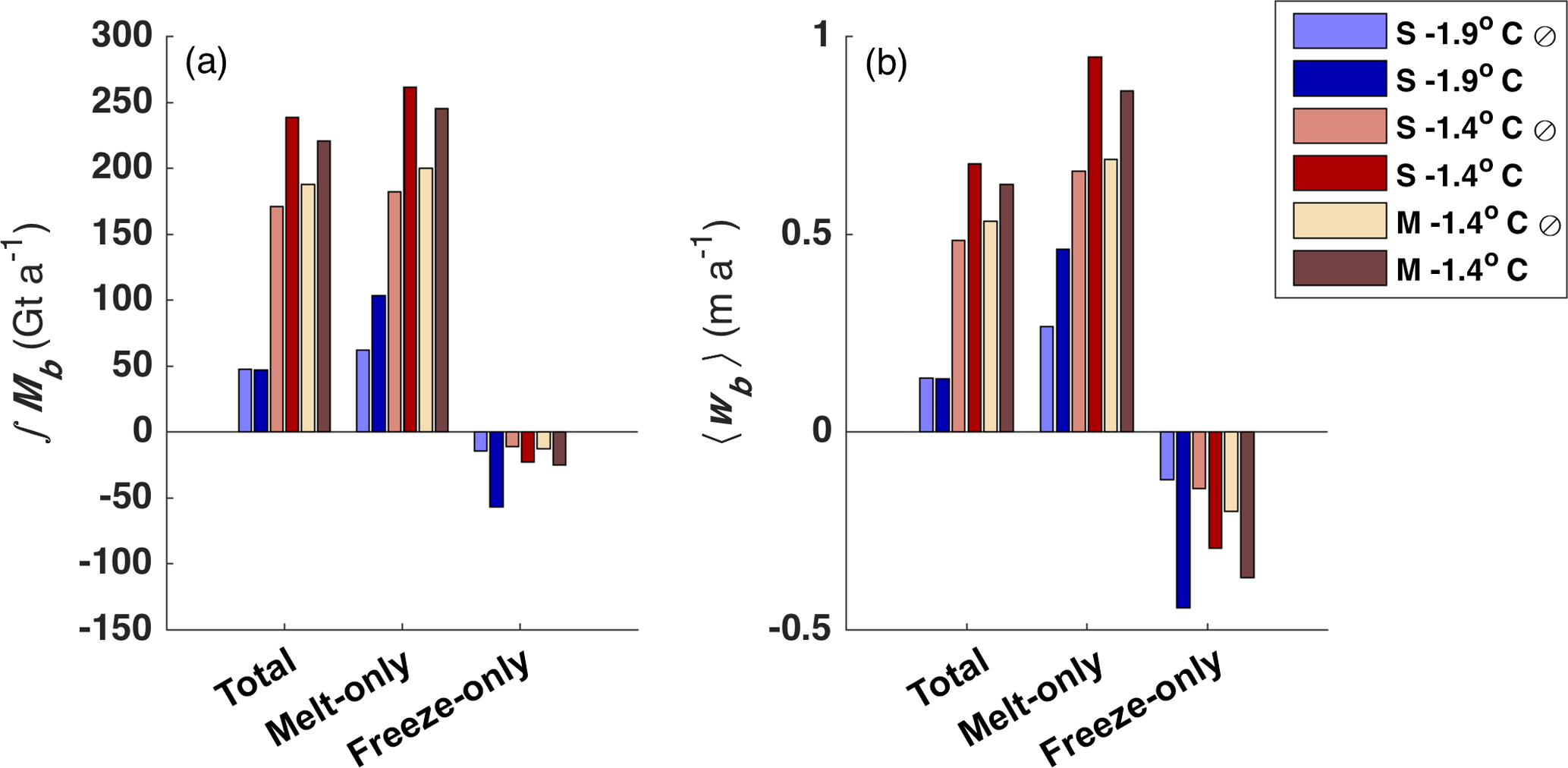
Figure 6(a) Integrated mass flux over total FRIS area, melt-only regions, and freeze-only regions for both no-tide (⊘) and tide-forced cases. (b) Same regions and runs as in (a) but showing FRIS-averaged basal melting.
Ocean temperature is the dominant control on total ice-shelf-integrated Mb and ice-shelf-averaged wb (Fig. 6; Table 2). Regardless of tides and geometry, warming the ocean inflow by 0.5 ∘C increases net mass loss by a factor of 3 to 5. The integrated mass gain due to freezing (marine ice formation) is insensitive to temperature for the no-tide cases but sensitive to temperature for the tide-forced cases (Fig. 6a), suggesting that accurate predictions of marine ice formation requires accurate representation of tidal currents in simulations.
Tides change the effect of ocean heat on distributions of Mb and wb. In particular, the addition of tides to the standard cold case (our approximation to the modern state) increases net freezing by a factor of 4 – almost exactly offsetting a factor-of-2 increase in mass loss in melt-only regions. For the warm cases, tides increase total mass loss in melting regions by about 20–40 %, with most of this increase occurring in South Channel and under FIS (see Fig. 5). In contrast to the cold case, the increases in net freezing in the warm cases is small compared with the increased mass loss, so the total basal mass loss for FRIS increases significantly when tides are added to a warm ocean.
Changing geometry has a much smaller but still significant effect on ice-shelf-integrated Mb and ice-shelf-averaged wb. In the no-tides simulations, the change from standard to modified geometry causes net mass loss to increase slightly, while the tide-forced cases show a slight decrease (Fig. 6). This change in sign in the mass loss anomaly is driven primarily by the anomalous behavior of South Channel and will be discussed in greater detail in Sect. 3.4 and 4.2.
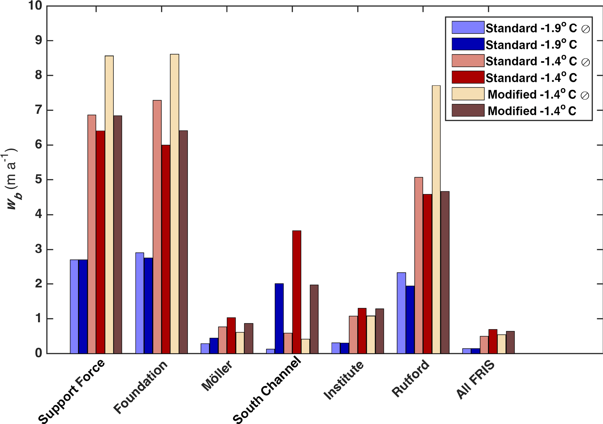
Figure 7Melt rates averaged over the last 12 months of steady state solutions in the standard cold, standard warm, and modified warm cases for some of the regions shown in Fig. 4 and for both no-tides (⊘) and tide-forced simulations. “All FRIS” duplicates the information shown by “total” in Fig. 6b.
3.4 Regional sensitivity of wb in the base simulations
Regional averages of wb (Fig. 7) indicate that basal mass loss near the grounding lines of major inflowing ice streams varies by an order of magnitude within a given simulation. The Support Force, Foundation, and Rutford ice streams show the largest values, exceeding 2 m a−1 for the standard cold cases with and without tide forcing. In contrast, modeled melt rates for the Möller and Institute ice streams are in the range of 0.28–0.44 m a−1 for the standard cold case runs.
For each ice-stream inlet, θinit is the primary control on melt rate near the grounding line, with mean melt rate approximately doubling from the standard cold case to the standard warm case. Tidal forcing is a secondary control that leads to either an increase or decrease in wb near grounding lines. For the Support Force, Foundation, and Rutford ice streams, adding tides reduces area-averaged melt rates, with the relative change being larger for the warm cases with both standard and modified geometry. The largest fractional change in melt rate due to tides occurs near the Rutford Ice Stream grounding line in the modified-geometry warm case, where adding tides reduces mean melt rate by 40 % from 7.7 to 4.6 m a−1.
South Channel is an exception to the general result that regional sensitivity of wb is more strongly affected by changes in θinit than tidal forcing. In this region, wb increases by roughly an order of magnitude between the no-tide and tide-forced simulations, whereas the fractional change due to θinit is much smaller, about a factor of 2 (Fig. 7). South Channel also experiences a large reduction (∼ 30 %) in regionally averaged wb in the modified warm tide-forced run compared with the standard warm tide-forced run. We attribute this change in wb to the reduction in tidal currents as geometry is changed (Fig. 3).
3.5 Ocean circulation within the FRIS cavity in the passive dye tracer simulations
General patterns of water mass circulation into and under FRIS are demonstrated by output from the 2-year simulations with passive-tracer dyes (see Sect. 2.3.3). We focus only on tide-forced simulations because, as discussed in Sect. 3.3 and by Makinson et al. (2011), tidal currents are known to be critical to patterns of basal melting beneath FRIS.

Figure 8Distribution of the dye concentration from the last time step and the upper model layer of the standard cold, tide-forced case described in Sect. 2.3.3. These distributions are from 2 years after the initiation of the model dye releases following 20 years of model circulation spin-up time. (a) Bulk dye representing penetration of water initially north of the FRIS ice front. (b–d) Meltwater dyes with sources in the Foundation, South Channel, and Rutford regions, respectively (see Fig. 4 for dye release regions). The white line across South Channel represents the location of the transects in Fig. 13.
3.5.1 Dye tracer circulation in the standard cold tide-forced case
The concentration of the open-ocean bulk dye tracer in the upper σ layer (Fig. 8a) reveals that the FRIS cavity has two different sources of heat inflow. The FIS and innermost RIS cavities are flooded by a southward transport of the open continental shelf waters across the FIS front, whereas the cavity circulation in the northeastern portion of RIS is dominated by incursions of water from across the RIS front. The latter inflow does not penetrate deep into the central and southern RIS within 2 years of simulation, although this is likely to be an artifact of the omission of the high-salinity shelf water that is known to form at the RIS front and is assumed to fuel gravity currents that reach the deep western grounding lines of RIS. In our simulations, the water entering through FIS circulates clockwise along the deep grounding line. After 2 years, some dye has reached as far west as Carlson inlet; however, very little of this dye is found under the central RIS north of the ice rises and rumples. The most direct impact of changes in open-ocean inflow is observed in the Support Force and Foundation inlets, as well as in South Channel.
Meltwater produced near the Foundation Ice Stream grounding line (Fig. 8b) reveals similar clockwise circulation, which is qualitatively similar to the plume flow described by Holland et al. (2007). This water reaches the western RIS ice front in about 2 years. Meltwater from Foundation inlet flows into all ice-stream inlets to the west of Foundation. The flow of this meltwater through South Channel is limited to the southern side of the channel.
Meltwater produced in South Channel also reaches all of the western RIS within 2 years (Fig. 8c), including much of the central region where refreezing occurs. Meltwater produced in Rutford inlet flows northward to the west of Korff Ice Rise (Fig. 8d).
These dye maps demonstrate that water found in contact with the ice shelf base in the uppermost layer, in a specific ice-stream inlet, is a mixture of the incoming high-salinity ocean water and meltwater that was produced at other inlets further upstream. As an important consequence, changes in meltwater production in different regions will alter the meltwater plume characteristics (e.g., temperature) experienced by downstream ice-stream grounding zones. In the following, it will be shown that the interactions within different grounding zone regions lead to non-local feedbacks of the melting response to changes in ocean temperatures and ice shelf geometry.
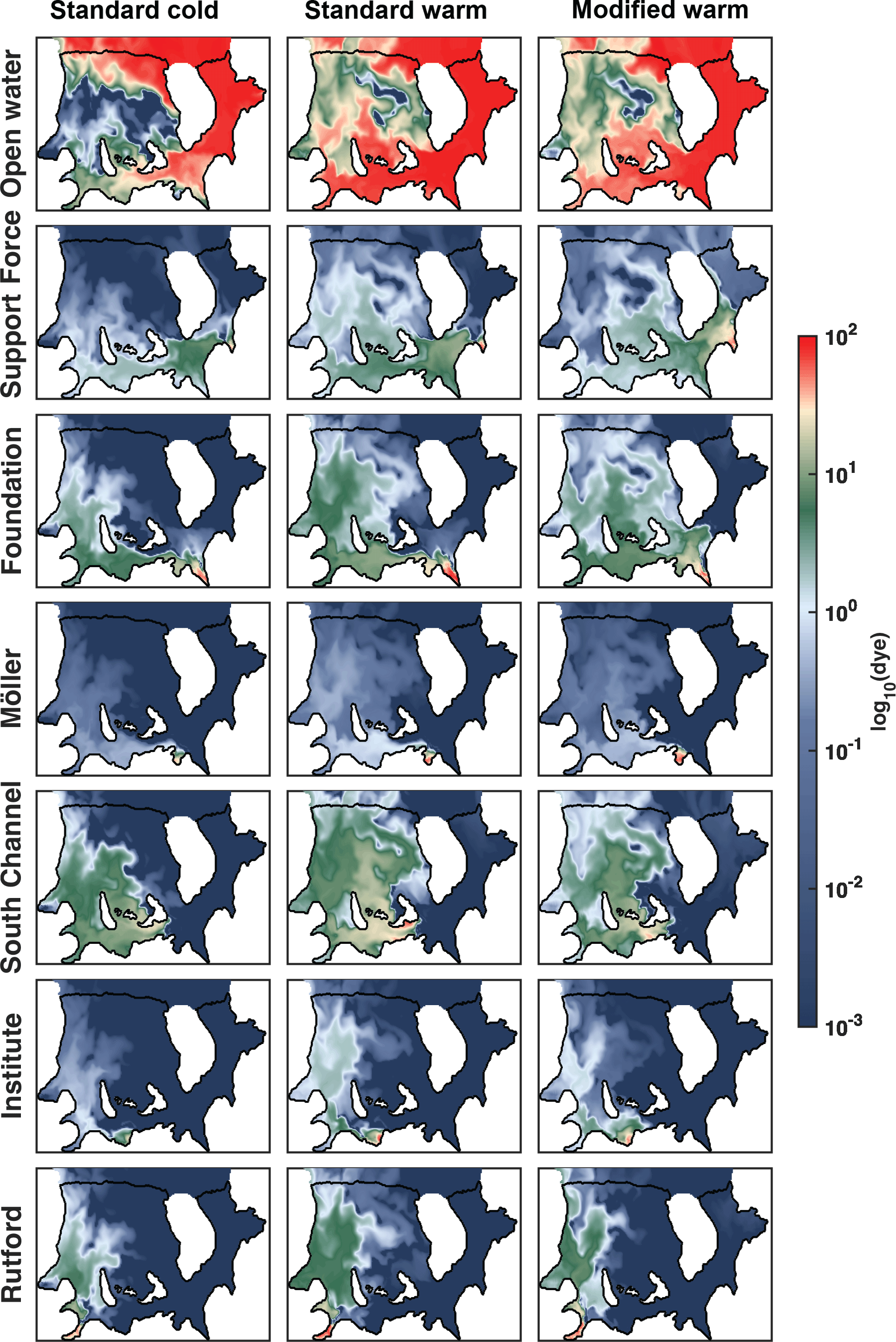
Figure 9A more expanded distribution of dye concentration than that shown in Fig. 8 to include all meltwater dyes in the three tide-forced base simulations. As in Fig. 8, dye concentrations are from the last 30-day average of upper model layer solutions from the runs described in Sect. 2.3.3. These distributions are from 2 years after initializing the dye release following 20 years of model circulation spin-up time. The left-hand column of this graphic includes the same four regional plots as shown in Fig. 8.
3.5.2 FRIS cavity dye tracer distribution for tide-forced cases
Comparisons of dye concentration maps after 2 years of integration for the three tide-forced simulations (Fig. 9) show differences that can be attributed both to θinit (comparing standard cold and standard warm cases) and to geometry (comparing standard warm and modified warm cases).
The stronger cavity circulation introduced by the amplification of net basal melting for the warmer ocean, ∘C, increases inflow through the FIS and into the RIS cavity (upper row of Fig. 9). Open-ocean water is present under most of RIS after 2 years in the standard warm case. The dye concentration of open-ocean water under the northern portion of RIS decreases as θinit increases, indicating that the stronger northward flow of meltwater in the warm case reduces the contribution of the direct open-ocean inflow to the northern RIS. This influence of θinit on strengthening the sub-ice shelf cavity circulation decreases slightly in the modified warm case, which shows less open water dye penetrating into the innermost RIS than the standard warm case solution (compare the two upper right subplots of Fig. 9).
Comparisons of meltwater dyes from ice-stream inlets and South Channel (lower six rows in Fig. 9) show, in all cases, more rapid ventilation of downstream regions when θinit is warmer. In these simulations, meltwater dyes are injected continuously at a rate that is scaled to the basal melt rate (Sect. 2.3.3). Relative dye concentrations at specific locations can, therefore, be interpreted as the relative values of meltwater from different sources with total meltwater plume concentration being an integration of the contributions from all upstream sources. Changes in the different runs reflect the response of the cavity circulation and changes in the meltwater production rate in the respective grounding zones. Meltwater from South Channel dominates the central RIS, although melting in the Foundation and Rutford inlets provides a substantial freshwater flux to the western RIS.
The changes in upper-ocean circulation caused by changes in geometry, seen by comparing the two warm cases in the last two columns of Fig. 9, are less obvious than the effect of changing temperature. Nevertheless, changing geometry has a significant regional effect. Foundation inlet meltwater spreads out more in the modified warm case than in the standard warm case as a result of increased dye transport through the channel between Henry Ice Rise and Berkner Island. South Channel meltwater concentrations are reduced in the modified warm case, which is consistent with the reduced melt rates in the region (Fig. 5). Similar to South Channel, Rutford inlet meltwater in the surface layer is also reduced for the modified-geometry case.
3.5.3 Regional meltwater dye comparison for tide-forced cases
Regional meltwater dye production and advection is evaluated from the surface levels of the Foundation, Möller, and South Channel inlet regions (as in Fig. 4). Figure 10 shows the integrated values over these regions for the standard cold, standard warm, and modified warm tide-forced cases. As described in Sect. 2.3.3, the meltwater dye from a particular region is a scaled quantity of wb that reflects the magnitude of meltwater produced in that region. The resulting passive dye is then transported through the domain through a combination of advection and mixing and acts as a proxy for the meltwater plume. In this section, we use the quantity of these meltwater tracers to demonstrate how meltwater circulation is affected by changes in θinit and geometry.
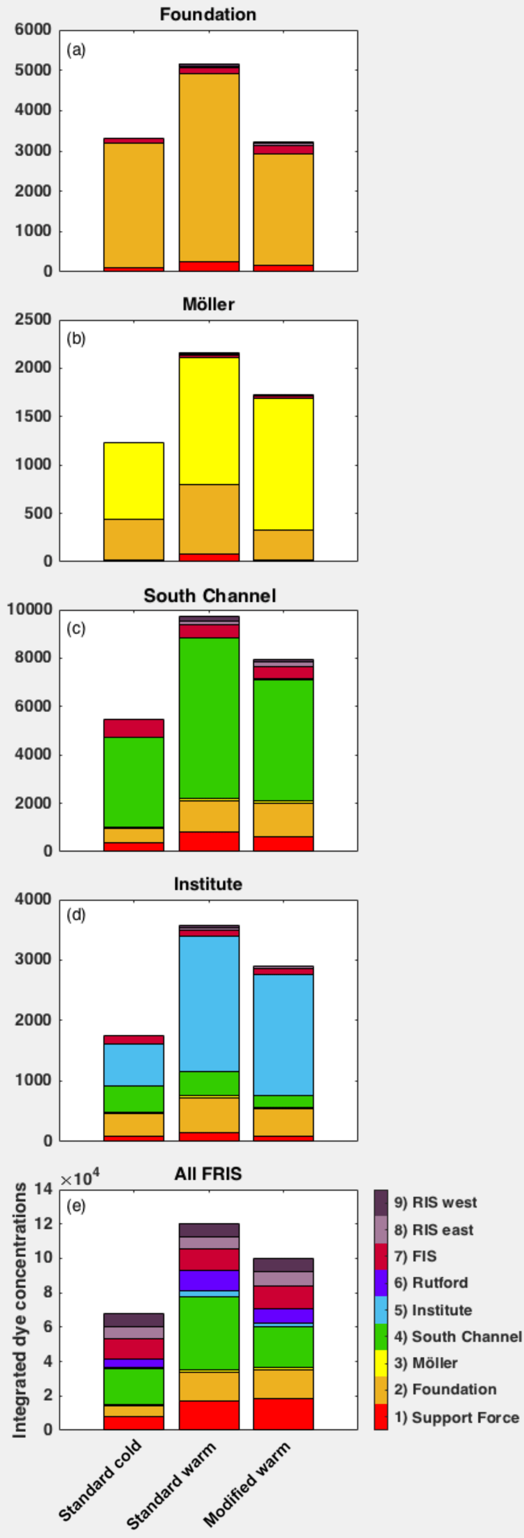
Figure 10Integrated meltwater dye (Sect. 2.3.3) by region for the tide-forced and base simulations, showing (a) the Foundation region, (b) the Möller region, (c) the South Channel region, (d) the Institute region, and (e) all of FRIS. Regions are shown in Fig. 4.
Foundation inlet shows an increase in the integrated meltwater dye with the 0.5 ∘C increase in θinit between the standard cold and standard warm cases (Fig. 10a). This increase in the integrated meltwater dye is not sustained with the change in cavity geometry. Instead, the net amount of the dye is reduced in the modified warm case such that the value of the integrated dye in the surface level more closely matches that of the standard cold case. This reduction in the integrated meltwater dye between the standard warm and modified warm case carries forward into the Möller region, where the reduction in the Foundation dye between the two cases is even greater than in Foundation inlet (compare Fig. 10a and b). At the same time, the reduction in the Foundation dye in the Möller region is somewhat compensated for by the Möller meltwater dye, which is consistent between the two warm cases (Fig. 10b). Overall, the Möller region appears to be less affected by the change in geometry than the Foundation region. Within South Channel, the influence of geometry on the quantity of the meltwater dye is compensated for by changes in circulation that allow for more Foundation dye in the surface level of South Channel in the modified warm case than the standard warm case (Fig. 10c). This increase in the surface level Foundation dye in South Channel is caused by changes in circulation that distribute the dye more evenly across South Channel in the modified warm case than in the standard warm case (Fig. 9).
These results highlight the fact that the regional sensitivities of the meltwater dye to θinit and geometry may influence but not necessarily determine the quantity and temperature of meltwater in downstream regions. This result reveals the degree to which θinit and cavity shape precondition the quantity and origin of meltwater in any given region. For example, the FRIS-integrated surface dye quantity (Fig. 10e) for Foundation and Support Force is equivalent between the standard warm and modified warm cases, even though there are strong regional variations in these cases (Fig. 10a–c). In addition, the FRIS-integrated values of meltwater dyes from the ice-front regions (RIS west, RIS east, and FIS) are similar among all cases while they differ among regions, showing greater amounts of dye in the Foundation, Möller, and South Channel regions for the warm cases than in the cold case. These regional and integrated changes demonstrate that the FRIS meltwater product is a result of regional feedbacks that are affected by a combination of production, mixing, and advection.
Table 2Values for integrated mass transport (Mb, Gt a−1) and FRIS-averaged basal melt rate (wb, m a−1) for the six runs shown in Fig. 6: standard cold no tides (S −1.9), standard cold tide forced (S −1.9), standard warm no tides (S −1.4), standard warm tide forced (S −1.4), modified warm no tides (M −1.4), and modified warm tide forced (M −1.4). The symbol “⊘” is used here to denote “no tides.”
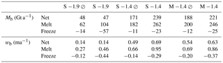
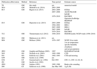
Table 3Publication sources and abbreviations used in Fig. 11. The methods for calculating melt rates are summarized as follows, following the nomenclature used in Table S2 of the Rignot et al. (2013) Supplement: ocean model (OM), standard glaciological method (GM), ocean observation (OO), and geophysical tracer (GT). The time period of observation(s) or forcing files is listed together with source of data or model output. n/a indicates studies in which time period is not applicable.
Our results show that tide forcing is important to FRIS ice–ocean interactions over a range of initial temperatures and with large variations in regional impacts. These results confirm an earlier study (Makinson et al., 2011) demonstrating that adding tide forcing to numerical models substantially increases basal melting along the deep grounding lines of FRIS and increases marine ice formation rates under RIS. Melting in these grounding-line regions has been shown to introduce a positive feedback to wb in response to increased basal slope and wct (Timmermann and Goeller, 2017). In this study, we address the combined influences from change in cavity shape, ocean warming, and tides. By carrying out simulations with different temperatures of water entering the sub-ice shelf cavity, and investigating potential changes to ice draft in a scenario with a warmer ocean, we have also shown that the spatial patterns of melting and refreezing are sensitive to complex feedbacks between basal melting, tidal currents, advection, and mixing.
The simplified forcing of our models prevents the development of some sub-ice shelf circulation features observed to be present in the modern state. The circulation under RIS is strongly affected by winter sea-ice formation and the associated production of high-salinity shelf water over the southern Weddell Sea continental shelf. Combined with larger-scale atmospheric forcing, these processes establish an east-to-west density gradient across the continental shelf (e.g., Foldvik et al., 1985; Nicholls et al., 2009) that drives a counterclockwise circulation with inflow in the Ronne Depression and a counterclockwise circulation around Berkner Island (Foldvik et al., 2001). Our idealized model also lacks the seasonal warming of the upper ocean near the ice front that leads to significant summer melting and rapid basal melting of the ice shelf frontal zone (e.g., Makinson and Nicholls, 1999; Joughin and Padman, 2003; Moholdt et al., 2014). Since we omit these forcings, our simulations do not capture these components of sub-ice shelf circulation. As a result, our cold-case simulations are “present-day” in terms of ocean thermal forcing but with circulation that is more representative of the future-warming scenario presented by Hellmer et al. (2012). These simplifications restrict the predictive capacity of our simulations but help us clarify the importance of tidal currents and tide-related feedbacks that affect future mass loss from FRIS and the adjacent buttressed, grounded ice.
We discuss the implications of our results by comparing our ice-shelf-averaged wb to other studies (Sect. 4.1), exploring regional influence of heat and velocity (Sect. 4.2), describing advection through South Channel (Sect. 4.3), relating our predicted change in ice shelf basal melt to regional changes in ice sheet mass balance (Sect. 4.4), and describing potential influences of marine ice accretion on ice sheet mass balance (Sect. 4.5).
4.1 Comparison of modeled, ice-shelf-averaged wb estimates with observations
The melt rate averaged over the area of an ice shelf is a common metric for evaluating ice shelf mass balance (e.g., Rignot et al., 2013; Depoorter et al., 2013). Our estimate of melt rate averaged over FRIS for the standard case is 0.14 m a−1 freshwater equivalent, which is equal to ∼ 48 Gt a−1 of net mass loss (Fig. 6 and Table 2). The range of values reported by other studies extends from 0.03 m a−1, the lower bound in Depoorter et al. (2013), to 0.55 m a−1 from the first oceanographically derived estimates (see Fig. 11 and Table 3; Jenkins, 1991; Jacobs et al., 1992). The range in estimates of wb is a result of variations in observation type and model choices. Estimating wb from observations typically requires averaging other ice shelf mass budget terms, derived from satellite observations and atmospheric models, over several years. Estimates from models are affected by the model setup.
Compared with the three most recent satellite-constrained estimates, our value is near the central estimate of 0.12 m a−1 of Depoorter et al. (2013) and near the lower limit of the ranges reported by Rignot et al. (2013) and Moholdt et al. (2014). Given the model simplifications discussed above, we regard the general agreement between our integrated mass loss and prior studies as evidence that our simulations are sufficiently realistic for further sensitivity studies and interpretation of the role of tides in FRIS evolution for future climate states.

Figure 11FRIS-averaged basal melt rate comparison between this study (TS) and others. Model results are shown as black dots while observations are shown as grey dots. Error bars for remote sensing observations are shown as black lines for M14 (Moholdt et al., 2014), R13 (Rignot et al., 2013) and D13 (Depoorter et al., 2013). Min and max values are connected by thick, solid, black lines to show the range of values reported by N03 (Nicholls et al., 2003) and G94 (Gammelsrød et al., 1994). A summary of the studies presented here and their abbreviations is provided in Table 2.
4.2 Sensitivity of wb to ΔT and surface currents
We explore the regional variations of thermal forcing (ΔT) and turbulent exchange (u∗) on wb using the 30-day averaged values from the end of each simulation to calculate ΔT and . Note that wb in the 30-day averaged model output is based on the average of instantaneous heat fluxes and, therefore, includes the model's knowledge of covariances between ΔT and on much shorter timescales. In contrast, is calculated from 30-day averaged u- and v-velocity components. We use a linear combination of non-tidal and tidal currents, U, given by
where is from Eq. (5), to represent the local forcing for turbulent exchange. For the no-tides cases, is zero and . We include in the tide-forced cases to more closely approximate the non-time-averaged relationship described by Eq. (1), because the 30-day average removes the tidal signal in ΔT and in the tide-forced cases.
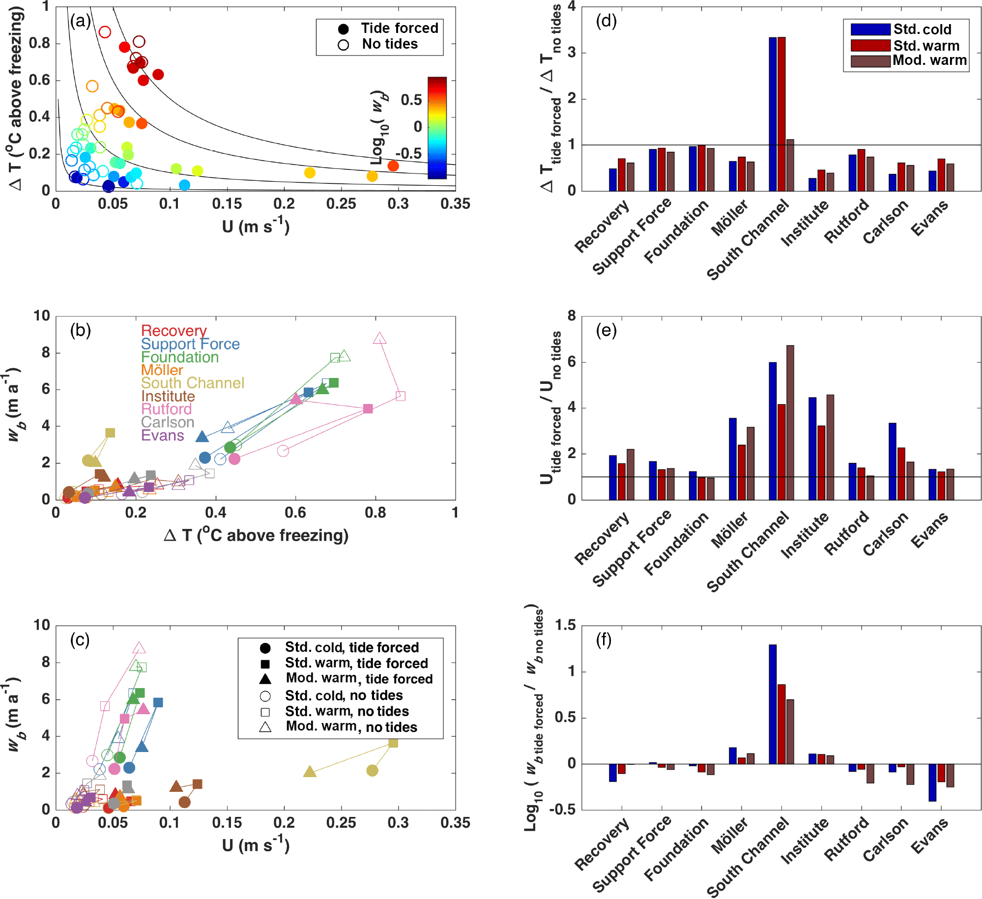
Figure 12Regional influences of ΔT and current speed on melt rates. Tide-forced cases are plotted using a solid marker style, ▪, and no-tide cases are plotted using an open marker style, □. (a) Current speed (U, Eq. 6) vs. thermal forcing (ΔT), color-coded according to melt rate (wb). Black contours follow (with c being a set of different scalars), along which constant values of wb (as in Sect. 3.2) are expected to be found. (b) ΔT vs. wb for each region. (c) U vs. wb for each region. (d) ΔT difference between no-tides and tide-forced cases such that positive values show where thermal forcing is stronger in the no-tides cases, (e) current speed difference between tide-forced (Utides) and no-tides (Uno tides) cases, and (f) wb difference between tide-forced and no-tides cases.
Comparisons of the six base simulations show that wb generally follows the expected functional dependence on ΔT and U (Fig. 12a): in all six cases, values of wb increase with stronger currents and more thermal forcing, with values roughly falling along lines of constant ΔT⋅U. In general, our values are in range of those shown by Holland et al. (2008), (compare their Fig. 1 with our Fig. 12b), although regional differences can be seen in the bivariate relationships between wb and either ΔT or U (Fig. 12b and c). Most ice-stream inlet averages show a similar increase in wb with respect to ΔT (Fig. 12b), suggesting that reasonable estimates of melt rate in the ice-stream inlets could be obtained from variability of ΔT and a constant, assumed low, value of U. South Channel and, to some degree, Institute inlet diverge from this relationship, demonstrating a larger variability in wb in relation to ΔT than is seen in other inlets (Fig. 12b). This larger variability in wb in South Channel arises because changes in modeled melt in this area are controlled primarily by changes in U (Fig. 12b).
Comparisons of the ratios for ΔT, U, and wb at each site between simulations without and with tides (Fig. 12d–f) show how each region responds to the combined effects of tide-induced changes in ocean conditions. With the exception of South Channel, adding tides always cools (decreases ΔT) the upper layer of ocean water adjacent to the ice base (Fig. 12d). On average, the largest reductions occur for RIS ice-stream inlets. We attribute this result to the cooling of water entering RIS inlets by inclusion of meltwater from upstream freshwater sources, with RIS inlets being influenced by rapid melting in the Support Force and Foundation inlets, as well as in South Channel (Figs. 8 and 9).
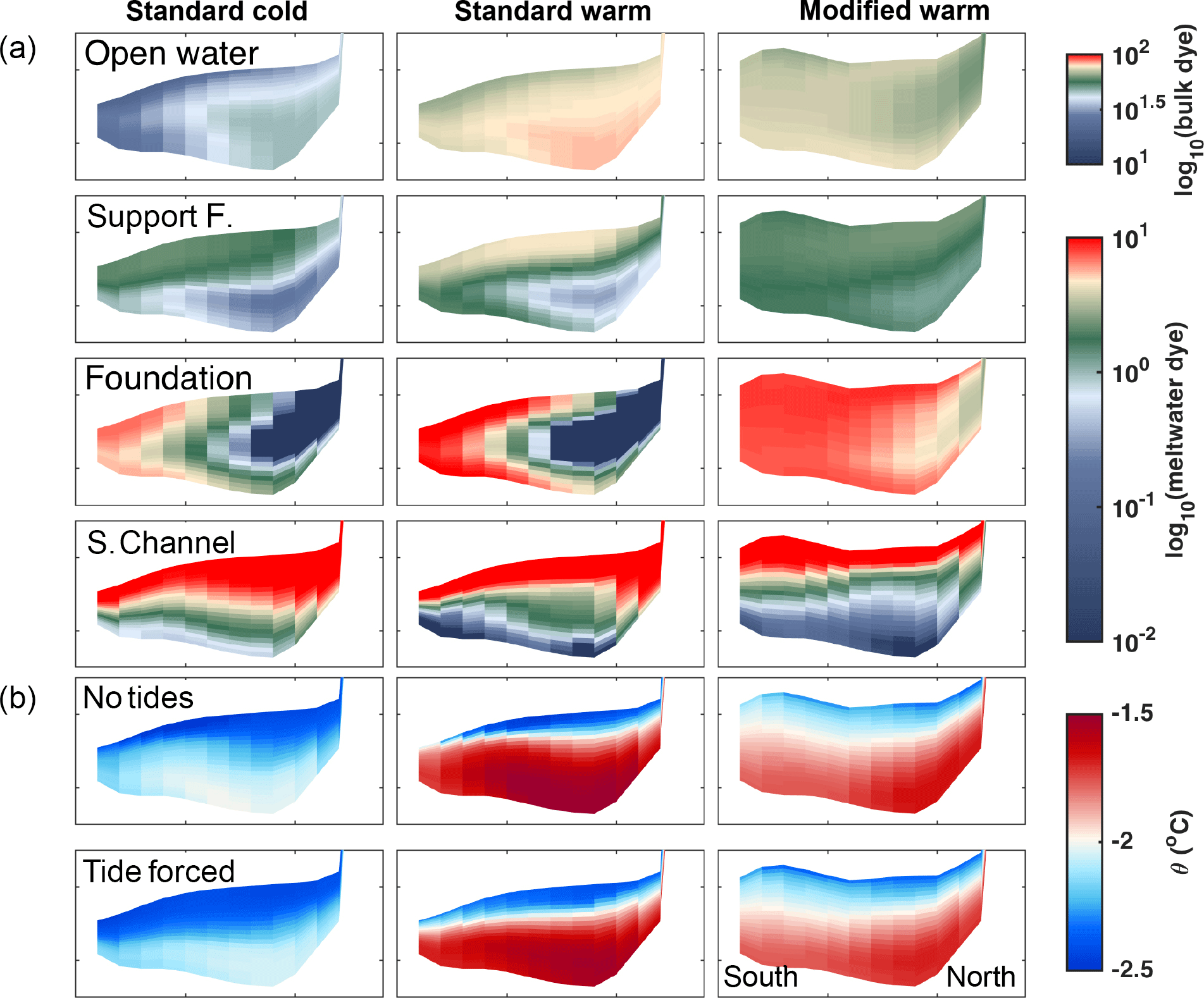
Figure 13Transects of dyes (a) and potential temperature (θ, b) across South Channel at the western tip of Henry Ice Rise. The upper four panels are for tide-forced runs only. Transect location is shown in Fig. 8.
The differences between the tide-forced and no-tide cases show up more strongly in the regionally averaged comparison of U (Eq. 6, Fig. 12e). In all regions, the effect of adding tides is greater for the cold standard cases than for warm standard cases. Since the value of in Eq. (5) is the same for the standard geometry runs, this difference represents the increase in the thermohaline-driven from the cold to warm cases.
The largest differences in amongst all three model runs are in the Möller, South Channel, and Institute inlets. For the warm cases, modifying the geometry increases the ratio of for these three regions even though tidal currents decrease (Fig. 3) as wct increases. This response implies that Uno tides also declines in the modified-geometry case. A decline in Uno tides in the modified geometry is consistent with a reduction in zice in the inlet regions, which would reduce the thermal forcing and, hence, reduce the ice pump circulation. If true, this feedback is an artifact of our model geometry, which excludes the possibility of deeper ice that could be exposed when the grounding line migrates due to the imposed thinning. Corollary evidence for this reduction in ice pump circulation is seen in the top row of Fig. 9.
The role of South Channel melt on cooling downstream ice-stream inlets, its sensitivity to tides, and tidal sensitivity to changing zice suggest that reliable predictions of change in modeled wb in the southern RIS ice streams for future climate scenarios depend on the correct representation of changes to South Channel geometry.
4.3 Role of advection through South Channel
As the maps of surface-layer dye tracers (Figs. 8 and 9) show, most water entering the FRIS cavity in our simulations flows southward under the FIS front and then circulates clockwise around the FIS and RIS grounding lines. A water parcel takes about 2 years to travel from the FIS front to the southwestern RIS region of Rutford inlet. During that time, each water parcel is subjected to mixing with meltwater, so the properties of water entering each inlet depend on the processes along the entire upstream path. Meltwater produced along each flow path continues to circulate clockwise with the inflowing warmer and saltier water that originated north of the ice front; see, e.g., dye distribution representing meltwater from Foundation inlet (Fig. 8b).
Water near the ice base in South Channel contains significant freshwater contributions from the Support Force and Foundation inlets, with a smaller contribution from Möller inlet (Fig. 9). A north–south transect across the western end of South Channel (location shown in Fig. 8 and transects in Fig. 13) shows that all water within that transect is colder than θinit. Although not shown, this water is also fresher, i.e., some meltwater from upstream is present at all depths. Furthermore, distributions of meltwater contributions from individual regional sources vary in the vertical and horizontal (Fig. 13), with the path-integrated buoyancy fluxes determining the meltwater fractions that drive stratification. The standard geometry simulations show a core of open water dye along the bottom and northeastern slope of the trough under South Channel. The Support Force dye is concentrated near the ice base, toward the southwestern end of the transect. The Foundation dye appears in both the surface and deep model layers, concentrated on the southern side of South Channel (see also Fig. 8b). The bifurcation of the Foundation dye in South Channel reflects two sources: one in which fairly pure inflow water melts ice in Foundation inlet and then flows directly into deeper portions of South Channel and the other in which the Foundation dye flows into Möller inlet and is mixed down to the bottom of Möller inlet, which shares a similar shoaling of bathymetry (and wct) as in South Channel (Fig. 2). As expected, the South Channel dye has the highest concentration in the surface waters of this transect.
The spatial pattern in dye distribution is fairly consistent between the warm and cold standard geometry cases, although much more open water dye from north of the ice front is present in the warm case. This quantitative difference is consistent with the overall understanding that warmer θinit drives a stronger thermohaline circulation that enhances cavity circulation and leads to a shorter residence time (Fig. 9).
More qualitative differences between simulations arise from the change in cavity shape. Except for the South Channel dye, the modified geometry shows more laterally uniform dye concentrations across the channel. Dye distribution remains vertically stratified in all three cases with the depth of the upper layer being similar in the standard warm and modified warm cases. However, even though the averaged wb in South Channel is similar between the standard cold and modified warm cases (Fig. 7), the South Channel meltwater product does not mix down as far in the modified warm case as it does in the standard cold case (Fig. 13), which we attribute to the much weaker tidal currents in this region (Fig. 3) for modified geometry.
Transects for dye tracers are only provided for the tide-forced cases. However, a comparison of temperature transects for the no-tides and tide-forced cases (Fig. 13) shows that the thermocline is deeper in the standard geometry tide-forced cases, with the thermocline most affected in the standard cold case. As shown in Fig. 12d, tides increase the thermal forcing in South Channel in the standard geometry by a factor of 3, while having a negligible effect on ΔT in the modified geometry. These results suggest that the lowered thermocline in this region is caused by tide-induced mixing rather than advection, so its depth responds to the reduced tidal currents in the modified warm case.
4.4 Implications of regional melt on ice sheet mass balance
Walker et al. (2008) showed that the spatial distribution of ice shelf melt rates was critical to the behavior of the buttressed grounded ice streams; for the same integrated mass loss from an ice shelf, grounded ice loss was significantly faster when the melting was concentrated near the grounding line. Gagliardini et al. (2010) confirmed this analysis and also noted that a grounded ice stream could thicken and its grounding line could advance (even when net melting increased) if the melt rate decreased near the grounding line. In the context of our study, the implication is that – even when the change in the area-averaged melt rate is small – substantial variability in melt rates near ice-stream grounding lines could still have a large impact on loss (or gain) of grounded ice.
In addition to being affected by the spatial distribution of wb, dynamic mass loss of grounded ice is also affected by bedrock slope and ice sheet topography. These factors introduce additional spatial heterogeneity in the influence of basal melting on overall mass loss from the grounded ice streams flowing into FRIS. Wright et al. (2014) used the BISICLES ice-sheet model to test the sensitivity of the grounded ice sheet to changes in FRIS mass loss at the grounding line. They found that the Institute and Möller ice streams are the most sensitive to changes in basal mass balance that might be caused by a warming ocean inflow. This result was confirmed by Martin et al. (2015) using the Parallel Ice Sheet Model (PISM). These two ice streams rest on top of steep reverse bed slopes with low basal roughness – conditions which have been shown to contribute to grounding line instability and retreat (Schoof, 2007). Furthermore, these ice streams are also sensitive to changes in the buttressing effect from ice shelf mass change around the Henry and Korff ice rises and the associated change in basal sliding over these ice rises. Our results indicate that tides currently exert a strong influence on basal mass balance in the area around the Henry and Korff ice rises (Fig. 5) by increasing melting in South Channel and increasing marine ice accretion north of the ice rises and Doake Ice Rumples.
Möller and Institute are among the lowest meltwater producing regions (Fig. 7) and receive the largest fraction of meltwater product from Foundation inlet basal melt (Fig. 10). The relative quantities of these meltwater products are sensitive to changes in advection and mixing imposed by changes in θinit and geometry (Sect. 3.5). As shown in Fig. 7, the 0.5 ∘C increase in θinit increases the Möller grounding-line region wb to 1.03 m a−1 (an increase of 134 %) and Institute grounding-line region wb to 1.30 m a−1 (an increase of 100 %) for the tide-forced cases. The grounding lines in these regions appear to be very sensitive to changes in θinit and less sensitive to changes in the cavity ocean circulation imposed by a change in model geometry. Even with Möller and Institute sensitivity to θinit, however, these inlets are buffered from variations in open-ocean heat due to the combined influence of circulation pathways and inflowing meltwater derivatives (Fig. 10).
Of the nine grounding-line regions explored in this study, Foundation inlet has the highest averaged melt rate of 2.76 m a−1 for the standard cold case (Fig. 7), a rate which more than doubles to 6.01 m a−1 when θinit increases from −1.9 to −1.4 ∘C. However, grounded ice mass flux from Foundation Ice Stream is less sensitive to changes in basal melting than Möller and Institute (Wright et al., 2014). According to the results presented in Wright et al. (2014), even the higher melt rate with the warmed ocean in our study is insufficient to drive grounding-line retreat and significant acceleration of grounded ice loss through Foundation inlet. Therefore, it is possible that the dominant effect on the grounded ice mass budget of large wb at Foundation is through the effect of Foundation inlet meltwater on downstream inlets, particularly Möller. As shown in the dye results presented in Sect. 3.5, Möller is somewhat isolated from FIS inflow but flooded by Foundation meltwater.
4.5 Implications of regional freeze conditions on ice sheet mass balance
As described in Sect. 3.2.1 and 3.2.2, refreezing occurs in our simulations throughout a large region of the central RIS. Refreezing in this region is qualitatively consistent with estimates of basal mass balance from satellite-based remote sensing (e.g., Joughin and Padman, 2003; Rignot et al., 2013; Moholdt et al., 2014). The extent of freezing conditions is important because marine ice accretion supports ice shelf stability through its effect on the mechanical properties of ice (Kulessa et al., 2014; McGrath et al., 2014; Li et al., 2017) and by altering the extent of grounding on topographic highs such as ice rises and rumples.
Our standard cold tide-forced case produces local maxima in marine ice growth rates in the northwestern RIS, the region northeast and east of Korff Ice Rise, and the region to the north and west of Henry Ice Rise (Fig. 5d). These regions of freezing are broadly consistent in all our model runs (Fig. 5) and the net mass increase in refreezing regions is increased when tide forcing is added (Fig. 6). Our standard cold tide-forced case has roughly 4 times more mass gain than the standard cold no-tides case, generally consistent with Makinson et al. (2011). In both warm cases, standard and modified geometry, adding tides increases net marine ice formation by a factor of 2. That is, tides will continue to be important for marine ice accretion beneath FRIS if ocean temperatures rise as predicted by Hellmer et al. (2012, 2017) and will, therefore, continue to play a role in FRIS stability.
The idealized modeling results presented here on the basal melting of FRIS, combined with ice-sheet model results reported by Wright et al. (2014), indicate that the response of the Antarctic Ice Sheet in the Weddell Sea sector to large-scale ocean circulation changes depends on several regional and local processes that combine to determine ocean state in individual ice-stream inlets. These processes include the tidal contribution to ocean mixing, advection of meltwater products into downstream inlets, and feedbacks (between advection, tides, and melting) as ice shelf draft evolves.
In general, tides increase the area-integrated mass loss from the entire FRIS, consistent with the findings of Makinson et al. (2011). However, unlike in Makinson et al. (2011), which showed that tides increased ice-shelf-averaged wb, our cold case ocean representing the modern state shows that increased basal melting with tides is completely offset by a factor-of-4 increase in freezing (marine ice formation) in the central Ronne Ice Shelf. It is only under the warm case conditions, in which these freezing conditions are reduced, that tides lead to an overall increase in ice-shelf-averaged wb. Our results show that ocean warming of 0.5 ∘C in the warm case increased total FRIS mass loss by a factor of ∼ 3.6 for the no-tides simulations (cf. Hellmer et al., 2012) and by a factor of ∼ 5.1 when tidal forcing was included.
The large-scale sub-ice shelf circulation in our idealized model is dominated by a southward inflow of open-ocean water across the Filchner Ice Shelf front and a clockwise circulation of this water along the southern grounding line. This clockwise sub-ice shelf circulation is, in part, a consequence of our simplified model forcing, which excludes some inflows that would be forced by realistic spatial and seasonal variability in the open ocean north of the ice shelf. Under this circulation regime, a water parcel takes about 2 years to travel from the Filchner ice front to the southwestern Ronne Ice Shelf.
On the regional scale, complex feedbacks occur between local processes such as tide-induced mixing and advection, so the temperature of a water parcel represents the upstream integrated history of mixing between the inflowing source water and basal meltwater. The temperature of the upper ocean layer adjacent to the ice shelf base is cooler when tide forcing is included, especially in the southwestern Ronne ice-stream inlets (Rutford, Carlson, and Evans). We attribute this cooling to the incorporation of meltwater from upstream sources, notably Foundation inlet and South Channel.
Our results show regionally variable responses to changes in tides, θinit, and cavity geometry that can be summarized as follows.
-
Meltwater plumes from basal melting introduce non-local feedbacks within an ice shelf in response to variations of inflowing ocean heat and melt-induced changes in ice draft.
-
Adding tide forcing to models increases wb under FIS and portions of RIS, with the largest increase within South Channel.
-
Adding tide forcing increases integrated marine ice formation for all three cases including the two warm cases. The tidal contribution to ice shelf dynamics will persist through future ocean warming of at least 0.5 ∘C and may increase ice sheet grounding and associated contact stresses in the region near the Henry and Korff ice rises as well as Doake Ice Rumples.
-
In some regions (e.g., South Channel), tides influence wb directly by changing the friction velocity; in other regions (e.g., Rutford), tides influence meltwater production through changes in θ by mixing along the upstream flow path.
-
The greatest fraction of meltwater in the Möller and Institute inlets are contributed by basal melting in Foundation inlet, indicating that increased meltwater production in one inlet may reduce melting in a downstream inlet.
The regional distributions of meltwater and wb are sensitive to the accuracy of our grids of seabed depth and wct, which are based on few passive seismic measurements in regions of strong model sensitivity (Fig. 3f). Distributions are also affected by the model configuration, including the neglect of atmospheric and sea-ice forcing, the choice of mixing schemes, and the thermodynamic exchange coefficients for the ice–ocean boundary layer parameterization. Nevertheless, our analysis shows that the interplay of tides, far-field thermal forcing, and the oceanic response to ice shelf geometry changes leads to complex and sometimes non-local interactions that alter the overall basal mass balance that effects melting near the grounding lines, thereby controlling the dynamical response of adjacent grounded ice streams.
Estimates of the future mass loss through the ice streams draining the West Antarctic Ice Sheet into Ronne Ice Shelf, in climate scenarios where the heat flux into the cavity under FRIS increases, are sensitive to how the ice draft in South Channel evolves. Under modern conditions and with the seabed and ice draft represented by the RTOPO-1 database, tides are a critical contributor to basal melting in that region. A warmer ocean will increase mass loss by basal melting that will lead to ice shelf thinning unless it is offset by increased inputs from ice advection and snowfall. However, this thinning then causes regional feedbacks that include (1) a reduction in basal melting in South Channel, as tidal currents weaken; (2) a change in circulation pathways with consequences for heat and meltwater transport; and, possibly, (3) a dynamic response of the grounded ice that may offset ocean-driven thinning of the ice shelf.
We conclude that it is not possible to predict the true effect of oceanic warming on ice thinning near individual ice-stream grounding lines without a better understanding of the feedbacks introduced by tidal forcing and circulation as a result of changes in wct. That is, as coupled ocean–ice-sheet models become a standard tool for projecting ice sheet response to changing climate, tides must be either explicitly modeled or represented by a parameterization that itself can evolve with time at a rate set by the evolution of the cavity. Furthermore, potential bottlenecks in sub-ice shelf circulation of ocean heat must be identified through improved surveys of seabed bathymetry which, when combined with the better-known ice shelf draft, determines both the tidal current speeds and the mean ocean circulation towards downstream sites including ice-stream inlets. The potential for future ocean warming, increased wb, and a corresponding mass loss that would cause around 1 m of sea level rise supports the need to augment measurements of the seabed bathymetry beneath FRIS, particularly within the ice-stream inlet regions and under South Channel.
Model output is available upon request.
The supplement related to this article is available online at: https://doi.org/10.5194/tc-12-453-2018-supplement.
RDM led the study. The simulations were designed by RDM and LP, implemented by RDM and SLH, and analyzed by RDM, LP, and TH. The paper was written by RDM, LP, and TH.
The authors declare that they have no conflict of interest.
We thank Mike Dinniman (Old Dominion University) for his invaluable help in
developing ROMS for use in simulating ice shelves, Scott Springer (Earth &
Space Research, ESR) for his help in creating the model
grid, and Keith Makinson and Hartmut Hellmer for their careful and detailed
reviews of this paper. Rachael Mueller is also grateful to Invent Coworking
for providing an excellent work space. This study was funded by NASA grants
NNX10AG19G and NNX13AP60G; NASA Earth and Space Science Fellowship,
07–Earth07F–0095; and The Research Council of Norway, program FRINATEK,
project Warm Deep Water on the Antarctic Continental Shelves no. 231549. This is ESR
publication number 160.
Edited by: G. Hilmar
Gudmundsson
Reviewed by: Hartmut Hellmer and Keith Makinson
Beckmann, A. and Haidvogel, D. B.: Numerical simulation of flow around a tall isolated seamount. Part 1: Problem formulation and model accuracy, J. Phys. Oceanogr., 23, 1736–1753, 1993.
Chapman, D.: Numerical treatment of cross-shelf open boundaries in a barotropic coastal ocean model, J. Phys. Oceanogr., 19, 384–391, 1985.
Darelius, E., Fer, I., and Nicholls, K. W.: Observed vulnerability of Filchner-Ronne Ice Shelf to wind-driven inflow of warm deep water, Nat. Commun., 7, 12300, https://doi.org/10.1038/ncomms12300, 2016.
Depoorter, M., Bamber, J., Griggs, J., Lenaerts, J., Ligtenberg, S., van den Broeke, M., and Moholdt, G.: Calving fluxes and basal melt rates of Antarctic ice shelves, Nature, 502, 89–92, https://doi.org/10.1038/nature12567, 2013.
Dinniman, M. S., Klinck, J. M., and Smith Jr., W. O.: Influence of sea ice cover and icebergs on circulation and water mass formation in a numerical circulation model of the Ross Sea, Antarctica. J. Geophys. Res., 112, C11013, https://doi.org/10.1029/2006JC004036, 2007.
Dinniman, M. S., Klinck, J. M., and Smith Jr., W. O.: A model study of Circumpolar Deep Water on the West Antarctic Peninsula and Ross Sea continental shelves, Deep-Sea Res. II., 58, 1508–1523, https://doi.org/10.1016/j.dsr2.2010.11.013, 2011.
Dupont, T. K. and Alley, R. B.: Assessment of the importance of ice-shelf buttressing to ice-sheet flow, Geophys. Res. Lett., 32, L04503, https://doi.org/10.1029/2004GL022024, 2005.
Flather, R.: A tidal model of the northwest European continental shelf, Memoires de la Societé Royale des Sciences de Liége, 6, 141–164, 1976.
Foldvik, A. and Kvinge, T.: Conditional instability of sea water at the freezing point, Deep Sea Res., 21, 169–174, 1974.
Foldvik, A., Gammelsrød, T., and Tørresen, T.: Circulation and water masses on the Southern Weddell Sea Shelf, in: Oceanology of the Antarctic Continental Shelf, Antarct. Res. Ser., vol. 43, edited by: Jacobs, S. S., 5–20, AGU, Washington, DC, 1985.
Foldvik, A., Gammelsrød, T., Nygaard, E., and Østerhus, S.: Current meter measurements near Ronne Ice Shelf, Weddell Sea: Implications for circulation and melting underneath the Filchner-Ronne ice shelves, J. Geophys. Res., 106, 4463–4477, 2001.
Gagliardini, O., Durand, G., Zwinger, T., Hindmarsh, R. C. A., and Le Meur, E.: Coupling of ice shelf melting and buttressing is a key process in ice-sheet dynamics, Geophys. Res. Lett., 37, L14501, https://doi.org/10.1029/2010GL043334, 2010.
Gammelsrød, T., Foldvik, A., Nøst, O. A., Foldvik, Ø., Anderson, L. G, Fogelqvist, E., Olsson, K., Tanhua, T. , Jones, E. P., and Østerhus, S.: Distribution of water masses on the continental shelf in the southern Weddell Sea, in: Polar oceans and their role in shaping the global environment, edited by: Johannessen, M., Muench, R. D., and Overland, J. E., 159–175, American Geophysical Union, Washington, DC, 1994.
Gerdes, R., Determann, J., and Grosfeld, K.: Ocean circulation beneath Filchner-Ronne Ice Shelf from three-dimensional model results, J. Geophys. Res., 104, 15827–15842, 1999.
Groh, A. and Horwath, M.: The method of tailored sensitivity kernels for GRACE mass change estimates, Geophys. Res. Abstr., 18, EGU2016–12065, 2016.
Haney, R. L.: On the pressure-gradient force over steep topography in sigma coordinate ocean models, J. Phys. Oceanogr., 21, 610–619, 1991.
Harig, C. and Simons, F. J.: Accelerated West Antarctic ice mass loss continues to outpace East Antarctic gains, Earth Planet. Sci. Lett., 415, 134–141, 2015.
Hellmer, H. H.: Impact of antarctic ice shelf basal melting on sea ice and deep ocean properties, Geophys. Res. Lett., 31, L10307, https://doi.org/10.1029/2004GL019506, 2004.
Hellmer, H. H. and Olbers, D. J.: A two-dimensional model for the thermohaline circulation under an ice shelf, Antarct. Sci., 1, 325–336, 1989.
Hellmer, H. H., Kauker, F., Timmermann, R., Determann, J., and Rae, J.: Twentyfirst–century warming of a large Antarctic ice-shelf cavity by a redirected coastal current, Nature, 485, 225–228, https://doi.org/10.1038/nature11064, 2012.
Hellmer, H. H., Kauker, F., Timmermann, R., and Hattermann, T.: The fate of the southern Weddell Sea continental shelf in a warming climate, J. Climate, 30, 4337–4350, 2017.
Holland, D. M. and Jenkins, A.: Modeling thermodynamic ice–ocean interactions at the base of an ice shelf, J. Phys. Oceanogr., 29, 1787–1800, 1999.
Holland, P. R., Feltham, D. L., and Jenkins, A.: Ice Shelf Water plume flow beneath Filchner-Ronne Ice Shelf, Antarctica, J. Geophys. Res., 112, C05044, https://doi.org/10.1029/2006JC003915, 2007.
Holland, P. R., Jenkins, A., and Holland, D. M.: The Response of Ice Shelf Basal Melting to Variations in Ocean Temperature, J. Climate, 21, 2558–2572, https://doi.org/10.1175/2007JCLI1909.1, 2008.
Jacobs, S. S., Hellmer, H. H., Doake, C. S. M., Jenkins, A., and Frolich, R. M.: Melting of ice shelves and the mass balance of Antarctica, J. Glaciol., 38, 375–387, 1992.
Jacobs, S., Giulivi, C., Dutrieux, P., Rignot, E., Nitsche, F., and Mouginot, J.: Getz Ice Shelf melting response to changes in ocean forcing, J. Geophys. Res.-Oceans, 118, 4152–4168, 2013.
Jenkins, A.: A one-dimensional model of ice shelf–ocean interaction, J. Geophys. Res.-Oceans, 96, 20671–20677, 1991.
Jenkins, A. and Jacobs, S.: Circulation and melting beneath George VI Ice Shelf, Antarctica, J. Geophys. Res., 113, C04013, https://doi.org/10.1029/2007JC004449, 2008.
Jenkins, A., Hellmer, H. H., and Holland, D. M.: The role of meltwater advection in the formulation of conservative boundary conditions at an ice-ocean interface, J. Phys. Oceanogr., 31, 285–296, 2001.
Jenkins, A., Nicholls, K. W., and Corr, H. F. J.: Observations and parameterization of ablation at the base of Ronne Ice Shelf, Antarctica, J. Phys. Oceanogr., 40, 2298–2312, 2010a.
Jenkins, A., Dutrieux, P., Jacobs, S. S., McPhail, S. D., Perrett, J. R., Webb, A. T., and White, D.: Observations beneath Pine Island Glacier in West Antarctica and implications for its retreat, Nat. Geosci., 3, 468–472, https://doi.org/10.1038/ngeo890, 2010b.
Joughin, I. and Padman, L.: Melting and freezing beneath Filchner-Ronne Ice Shelf, Antarctica, Geophys. Res. Lett., 30, 1477, https://doi.org/10.1029/2003GL016941, 2003.
Joughin, I., Smith, B. E., and Medley, B.: Marine ice sheet collapse potentially under way for the Thwaites Glacier basin, West Antarctica, Science, 344, 735–738, 2014.
Khazendar, A., Rignot, E., Schroeder, D. M., Seroussi, H., Schodlok, M. P., Scheuchl, B., Mouginot, J., Sutterley, T. C., and Velicogna, I.: Rapid submarine ice melting in the grounding zones of ice shelves in West Antarctica, Nat. Commun., 7, 13243, https://doi.org/10.1038/ncomms13243, 2016.
Kulessa, B., Jansen, D., Luckman, A. J., King, E., and Sammonds, P. R.: Marine ice regulates the future stability of a large Antarctic ice shelf, Nat. Commun., 5, 3707, https://doi.org/10.1038/ncomms4707, 2014.
Li, R., Xiao, H., Liu, S., and Tong, X.: A Systematic Study of the Fracturing of Ronne–Filchner Ice Shelf, Antarctica, Using Multisource Satellite Data from 2001 to 2016, The Cryosphere Discuss., https://doi.org/10.5194/tc-2017-178, in review, 2017.
MacAyeal, D. R: Thermohaline circulation below the Ross Ice Shelf: A consequence of tidally induced vertical mixing and basal melting, J. Geophys. Res., 89, 597–606, 1984.
Makinson, K. and Nicholls, K.: Modeling Tidal currents beneath Filchner-Ronne Ice Shelf and on the adjacent continental shelf: Their effect on mixing and transport, J. Geophys. Res., 104, 13449–13465, 1999.
Makinson, K., Schröder, M., and Østerhus, S.: Effect of critical latitude and seasonal stratication on tidal current profiles along Ronne Ice Front, Antarctica, J. Geophys. Res.-Oceans, 111, C03022, https://doi.org/10.1029/2005JC003062, 2006.
Makinson, K., Holland, P., Jenkins, A., Nicholls, K. W., and Holland, D. M.: Influence of tides on melting and freezing beneath Filchner-Ronne Ice Shelf, Antarctica, Geophys. Res. Lett., 38, L06601, https://doi.org/10.1029/2010GL046462, 2011.
Marchesiello, P., McWilliams, J. C., and Shchepetkin, A.: Open boundary conditions for long–term integration of regional oceanic models, Ocean Model., 3, 1–20, 2001.
Martin, M. A., Levermann, A., and Winkelmann, R.: Comparing ice discharge through West Antarctic Gateways: Weddell vs. Amundsen Sea warming, The Cryosphere Discuss., https://doi.org/10.5194/tcd-9-1705-2015, 2015.
McGrath, D., Steffen, K., Holland, P. R., Scambos, T., Rajaram, H., Abdalati, W., and Rignot, E.: The structure and effect of suture zones in the Larsen C Ice Shelf, Antarctica, J. Geophys. Res.-Earth, 119, 588–602, https://doi.org/10.1002/2013JF002935, 2014.
McPhee, M. G., Morison, J. H., and Nilsen, F.: Revisiting heat and salt exchange at the ice-ocean interface: Ocean flux and modeling considerations, J. Geophys. Res.-Oceans, 113, C06014, https://doi.org/10.1029/2007JC004383, 2008.
Mengel, M., Feldmann, J., and Levermann, A.: Linear sea–level response to abrupt ocean warming of major West Antarctic ice basin, Nat. Clim. Change, 6, 71–74, https://doi.org/10.1038/nclimate2808, 2016.
Moholdt, G., Padman, L., and Fricker, A.: Basal mass budget of Ross and Filchner-Ronne ice shelves, Antarctica, derived from Lagrangian analysis of ICESat altimetry, J. Geophys. Res.-Earth, 119, 2361–2380, 2014.
Mouginot, J., Rignot, E., and Scheuchl, B.: Sustained increase in ice discharge from the Amundsen Sea Embayment, West Antarctica, from 1973 to 2013, Geophys. Res. Lett., 41, 1576–1584, https://doi.org/10.1002/2013GL059069, 2014.
Mueller, R. D.: The effects of thermodynamic parameterizations, ice shelf geometry, and tides on modeled basal melting of Weddell Sea ice shelves, doctoral dissertation, Oregon State University, available at: http://ir.library.oregonstate.edu/concern/graduate_thesis_or_dissertations/3x816s04t (last access: 30 January 2018), 2014.
Mueller, R. D., Padman, L., Dinniman, M. S., Erofeeva, S. Y., Fricker, H. A., and King, M. A.: Impact of tide–topography interactions on basal melting of Larsen C Ice Shelf, Antarctica, J. Geophys. Res., 117, C05005, https://doi.org/10.1029/2011JC007263, 2012.
Nicholls, K. W. and Østerhus, S.: Interannual variability and ventilation timescales in the ocean cavity beneath Filchner-Ronne Ice Shelf, Antarctica, J. Geophys. Res., 109, C04014, https://doi.org/10.1029/2003JC002149, 2004.
Nicholls, K. W., Østerhus, S., Makinson, K., and Johnson, M. R.: Oceanographic conditions south of Berkner Island, beneath Filchner-Ronne Ice Shelf, Antarctica, J. Geophys. Res.-Oceans, 106, 11481–11492, 2001.
Nicholls, K. W., Padman, L., Schröder, M., Woodgate, R. A., Jenkins, A., and Østerhus, S.: Water Mass Modification Over the Continental Shelf North of Ronne Ice Shelf, Antarctica, J. Geophys. Res.-Oceans, 108, 3260, https://doi.org/10.1029/2002JC001713, 2003.
Nicholls, K. W., Østerhus, S., Makinson, K., and Gammelsrød, T., and Fahrbach, E.: Ice-ocean processes over the continental shelf of the southern Weddell Sea, Antarctica: A review, Rev. Geophys., 47, RG3003, https://doi.org/10.1029/2007RG000250, 2009.
Padman, L., Fricker, H. A., Coleman, R., Howard, S., and Erofeeva, S.: A new tidal model for the Antarctic ice shelves and seas, J. Glaciol., 34, 247–254, 2002.
Padman, L., Costa, D. P., Dinniman, M. S., Fricker, H. A., Goebel, M. E., Huckstadt, L. A., Humbert, A., Joughin, I., Lenaerts, J. T. M., Ligtenberg, S. R. M., Scambos, T., and Van den Broeke, M. R.: Oceanic controls on mass balance of Wilkins Ice Shelf, Antarctica, J. Geophys. Res., 117, C01010, https://doi.org/10.1029/2011JC007301, 2012.
Paolo, F. S., Fricker, H. A., and Padman, L.: Volume loss from Antarctic ice shelves is accelerating, Science, 348, 327–331, 2015.
Padman, L., Siegfried, M. R., and Fricker, H. A.: Ocean Tide Influences on the Antarctic and Greenland Ice Sheets, Rev. Geophys., 56, https://doi.org/10.1002/2016RG000546, 2018.
Pritchard, H. D., Arthern, R. J., Vaughan, D. G., and Edwards, L. A.: Extensive dynamic thinning on the margins of the Greenland and Antarctic ice sheets, Nature, 461, 971–975, https://doi.org/10.1038/nature08471, 2009.
Pritchard, H. D., Ligtenberg, S. R. M., Fricker, H. A., Vaughan, D. G., van den Broeke, M. R., and Padman, L.: Antarctic ice-sheet loss driven by basal melting of ice shelves, Nature, 484, 502–505, https://doi.org/10.1038/nature10968, 2012.
Raymond, W. H. and Kuo, H. L.: A radiation boundary condition for multi-dimensional flows, Q. J. Roy. Meteor. Soc., 110, 535–551, 1984.
Rignot, E. and Jacobs, S. S.: Rapid bottom melting widespread near Antarctic Ice Sheet grounding lines, Science, 296, 2020–2023, https://doi.org/10.1126/science.1070942, 2002.
Rignot, E., Mouginot, J., and Scheuchl, B.: Ice-shelf melting around Antarctica, Science, 341, 266–270, https://doi.org/10.1126/science.1235798, 2013.
Rignot, E., Mouginot, J., Morlighem, M., Seroussi, H., and Scheuchl, B.: Widespread, rapid grounding line retreat of Pine Island, Thwaites, Smith, and Kohler glaciers, West Antarctica, from 1992 to 2011, Geophys. Res. Lett., 41, 3502–3509, 2014.
Robertson, R., Padman, L., and Egbert, G.: Tides in the Weddell Sea, in: Oceanology of the Antarctic Continental Shelf, Antarct. Res. Ser., vol. 75, edited by: Jacobs, S. and Weiss, R., 341–369, AGU, Washington, DC, 1998.
Rosier, S. H. R., Green, J. A. M., Scourse, J. D., and Winkelmann, R.: Modeling Antarctic tides in response to ice shelf thinning and retreat, J. Geophys. Res.-Oceans, 119, 87–97, 2014.
Ross, N., Bingham, R. G., Corr, H. F., Ferraccioli, F., Jordan, T. A., Le Brocq, A., Rippin, D. M., Young, D., Blankenship, D. D., and Siegert, M. J.: Steep reverse bed slope at the grounding line of the Weddell Sea sector in West Antarctica, Nat. Geosci., 5, 393–396, 2012.
Scambos, T. A., Bohlander, J. A., Shuman, C. A., and Skvarca, P.: Glacier acceleration and thinning after ice shelf collapse in the Larsen B embayment, Antarctica, Geophys. Res. Lett., 31, L18402, https://doi.org/10.1029/2004GL020670, 2004.
Schlosser, P., Bayer, R., Foldvik, A., Gammelsrød, T., Rohardt, G., and Münnich, K. O.: Oxygen 18 and Helium as tracers of ice shelf water and water/ice interactions in the Weddell Sea, J. Geophys. Res., 95, 3253–3263, 1990.
Schmidtko, S., Heywood, K. J., Thompson, A. F., and Aoki, S.: Multidecadal warming of Antarctic waters, Science, 346, 1227–1231, 2014.
Schodlok, M. P., Menemenlis, D., Rignot, E., and Studinger, M.: Sensitivity of the ice-shelf/ocean system to the sub-ice-shelf cavity shape measured by NASA IceBridge in Pine Island Glacier, West Antarctica, Ann. Glaciol., 53, 156–162, 2012.
Schoof, C.: Ice sheet grounding line dynamics: Steady states, stability, and hysteresis, J. Geophys. Res.-Earth, 112, F03S28, https://doi.org/10.1029/2006JF000664, 2007.
Shchepetkin, A. F. and McWilliams, J. C.: A method for computing horizontal pressure–gradient force in an oceanic model with a nonaligned vertical coordinate, J. Geophys. Res.-Oceans, 108, 3090, https://doi.org/10.1029/2001JC001047, 2003.
Shchepetkin, A. F. and McWilliams, J. C.: Correction and commentary for “Ocean forecasting in terrain–following coordinates: Formulation and skill assessment of the regional ocean modeling system” by Haidvogel et al., J. Comp. Phys., 227, 3595–3624, J. Comp. Phys., 228, 8985–9000, https://doi.org/10.1016/j.jcp.2009.09.002, 2009.
Sutterley, T. C., Velicogna, I., Rignot, E., Mouginot, J., Flament, T., van den Broeke, M. R., van Wessem, J. M., and Reijmer, C. H.: Mass loss of the Amundsen Sea Embayment of West Antarctica from four independent techniques, Geophys. Res. Lett., 41, 8421–8428, https://doi.org/10.1002/2014GL061940, 2014.
Timmermann, R. and Goeller, S.: Response to Filchner–Ronne Ice Shelf cavity warming in a coupled ocean–ice sheet model – Part 1: The ocean perspective, Ocean Sci., 13, 765–776, https://doi.org/10.5194/os-13-765-2017, 2017.
Timmermann, R. and Hellmer, H.: Southern Ocean warming and increased ice shelf basal melting in the twenty–first and twenty–second centuries based on coupled ice-ocean finite–element modelling, Ocean Dynam., 63, 1011–1026, https://doi.org/10.1007/s10236-013-0642-0, 2013.
Timmermann, R., Le Brocq, A., Deen, T., Domack, E., Dutrieux, P., Galton-Fenzi, B., Hellmer, H., Humbert, A., Jansen, D., Jenkins, A., Lambrecht, A., Makinson, K., Niederjasper, F., Nitsche, F., Nøst, O. A., Smedsrud, L. H., and Smith, W. H. F.: A consistent data set of Antarctic ice sheet topography, cavity geometry, and global bathymetry, Earth Syst. Sci. Data, 2, 261–273, https://doi.org/10.5194/essd-2-261-2010, 2010.
Timmermann, R., Wang, Q., and Hellmer, H. H.: Ice-shelf basal melting in a global finite–element sea-ice/ice-shelf/ocean model, Ann. Glaciol., 53, 303–314, https://doi.org/10.3189/2012AoG60A156, 2012.
Walker, R. T., Dupont, T. K., Parizek, B. R., and Alley, R. B.: Effects of basal–melting distribution on the retreat of ice-shelf grounding lines, Geophys. Res. Lett., 350, L17503, https://doi.org/10.1029/2008GL034947, 2008.
Wright, A. P., Le Brocq, A. M., Cornford, S. L., Bingham, R. G., Corr, H. F. J., Ferraccioli, F., Jordan, T. A., Payne, A. J., Rippin, D. M., Ross, N., and Siegert, M. J.: Sensitivity of the Weddell Sea sector ice streams to sub-shelf melting and surface accumulation, The Cryosphere, 8, 2119–2134, https://doi.org/10.5194/tc-8-2119-2014, 2014.