the Creative Commons Attribution 4.0 License.
the Creative Commons Attribution 4.0 License.
 | 21 Dec 2018
Estimation of sea ice parameters from sea ice model with assimilated ice concentration and SST
Siva Prasad
Igor Zakharov
Peter McGuire
Desmond Power
Martin Richard
A multi-category numerical sea ice model CICE was used along with data assimilation to derive sea ice parameters in the region of Baffin Bay and Labrador Sea. The assimilation of ice concentration was performed using the data derived from the Advanced Microwave Scanning Radiometer (AMSR-E and AMSR2). The model uses a mixed-layer slab ocean parameterization to compute the sea surface temperature (SST) and thereby to compute the freezing and melting potential of ice. The data from Advanced Very High Resolution Radiometer (AVHRR-only optimum interpolation analysis) were used to assimilate SST. The modelled ice parameters including concentration, ice thickness, freeboard and keel depth were compared with parameters estimated from remote-sensing data. The ice thickness estimated from the model was compared with the measurements derived from Soil Moisture Ocean Salinity – Microwave Imaging Radiometer using Aperture Synthesis (SMOS–MIRAS). The model freeboard estimates were compared with the freeboard measurements derived from CryoSat2. The ice concentration, thickness and freeboard estimates from the model assimilated with both ice concentration and SST were found to be within the uncertainty in the observation except during March. The model-estimated draft was compared with the measurements from an upward-looking sonar (ULS) deployed in the Labrador Sea (near Makkovik Bank). The difference between modelled draft and ULS measurements estimated from the model was found to be within 10 cm. The keel depth measurements from the ULS instruments were compared to the estimates from the model to retrieve a relationship between the ridge height and keel depth.
- Article
(8246 KB) - Full-text XML
- BibTeX
- EndNote


Regional sea ice forecasting is important for climate studies, operational activities including navigation, exploration of offshore mineral resources and ecological applications; e.g. the North Water Polynya in Baffin Bay provides a warm environment for marine animals (Stirling, 1980).
Sea ice is a heterogeneous media, making it practically difficult for remote sensing instruments to measure the ice thickness, freeboard and ridge parameters (Carsey, 1992). The climate forecast researchers and operational ice modelling communities depend on numerical modelling techniques implementing the physical process of atmosphere and ocean on large-scale computational platforms along with data assimilation methods to retrieve the information on sea ice parameters. Data assimilation methods can provide more accurate initial conditions for forecasting systems (Caya et al., 2006, 2010). The estimation of sea ice parameters is a challenging problem in the region of Baffin Bay and the Labrador Sea due to the high interannual variability of sea ice in this area (Fenty and Heimbach, 2013).
Previous sea ice modelling and assimilation studies at the Canadian Ice Service (CIS) (Sayed and Carrieres, 1999) provided an overview of an operational ice model coupled with atmospheric and ocean modules. The research (Sayed et al., 2001) compared the evolution of ice thickness distributions followed by the development of an operational ice dynamics model for CIS (Sayed et al., 2002). The CIS used the model developed by Sayed and Carrieres (1999); Sayed et al. (2002) to study the ice thickness distribution in the Gulf of St Lawrence (Kubat et al., 2010) These modelling studies were also improved by the data assimilation methods (Caya et al., 2006, 2010). The Community Ice Ocean Model (CIOM) by Caya et al. (2006) used the Princeton Ocean Model for the simulation of ocean parameters and a multi-category ice model. The total ice fraction retrieved from the Special Sensor Microwave/Imager (SSM/I) was assimilated into CDOM using a 3-D variational (3DVAR) technique (Caya et al., 2006) to estimate the ice concentration. The ice concentration estimates were further improved by assimilating information from both daily ice charts and RADARSAT (Caya et al., 2010). Assimilation studies by Lindsay and Zhang (2006) showed significant improvement in assimilated ice concentration but with a large bias in the ice thickness pattern.
Karvonen et al. (2012) presented a method for ice concentration and thickness analysis by combining the modelling of sea ice thermodynamics and the detection of ice motion by space-borne synthetic aperture radar (SAR) data from RADARSAT-1 and RADARSAT-2. The method showed promising results for sea ice concentration and ice thickness estimates. In another study, Ocean and Sea Ice Satellite Application Facility (OSI SAF) data were assimilated into the Regional Ocean Modelling System (ROMS) for simulating sea ice concentration and produced better results than the simulation without assimilation (Wang et al., 2013). Ice concentration and extent were overestimated in the assimilated model, probably due to the bias in atmospheric forcing, underestimation of heat flux and over- and underestimation of sea ice growth and melt processes.
Sea ice models can be coupled to ocean and atmosphere models, but they can also be run in a stand-alone mode by prescribing the atmospheric and ocean conditions. The literature does not provide details and discussion on regional implementation and results for stand-alone models. The 3D-CEMBS is an eco-hydrodynamic model that includes a coupled POP-CICE model for operational forecasting implementation of the CICE model on a regional scale. The implementation on the regional scale of the ice component and the validation work is still ongoing (Dzierzbicka-Głowacka et al., 2013). The advantage of the sea ice model, CICE version 5.1.2 (Hunke et al., 2015), is the stand-alone capability. Here we use a combination of modelling using the stand-alone sea ice model, CICE, and the combination of optimal interpolation and nudging methods (Lindsay and Zhang, 2006; Wang et al., 2013) to assimilate ice concentration. The optimal interpolation and nudging method is also used to assimilate SST estimated by a slab ocean parameterization in the sea ice model. The optimal interpolation method is computationally inexpensive and was shown to provide better estimates than the non-assimilated model (Wang et al., 2013). The simulated sea ice parameters are then validated with the observations in the region of the Baffin Bay and the Labrador Sea. This work uses a high-resolution model configuration which was previously described in the work of Prasad et al. (2015). The changes in ice concentration were taken into account to estimate the changes in the ice volume and thereby the thickness estimates. The ice prediction models such as Regional Ice Prediction System (RIPS) (Lemieux et al., 2016) limits the discussion on ice concentration estimates from the model. In this work, in addition to validation of the ice concentration we also discuss the effect of the assimilation on ice thickness, freeboard, draft and keel depth. Since freeboard, draft and keel are functions of ice concentration and ice volume it is reasonable to compare the model values with corresponded observations. The work suggests a methodology to extract the level ice draft and keel depth information from upward-looking sonar (ULS) measurements, which was then used to describe the relationship between ridge and keel.
The sea ice model was implemented on a regional scale of about 10 km orthogonal curvilinear grids with a slab ocean mixed-layer parameterization. Density-based criteria were used as in Prasad et al. (2015) to compute the mixed-layer depth and thereby compute the SST and the potential to grow or melt sea ice. The assessment of the non-assimilated model of the sea ice concentration and its seasonal means showed that the error associated with the model is mostly spread across the area of the North Water Polynya and the Davis Strait where the interaction of cold and warm water is frequent. In the present study, a data assimilation module is also introduced.
The surface atmospheric forcing is from high-resolution North American Regional Reanalysis (NARR) data (Mesinger et al., 2006). The ocean forcing is from various sources: currents from Climate Forecast System Reanalysis (CFSR), salinity from World Ocean Atlas, WOA-2013 (Levitus and Mishonov, 2013), and mixed-layer depth (MLD) computed from WOA-2013 (Prasad et al., 2015). Prasad et al. (2015) used a density criteria of 0.2 kg m−3 at 10 m depth; the other models such as RIPS by CIS (Lemieux et al., 2016) use a density criteria of 0.01 m−3 from the ocean surface. Atmospheric and ocean forcing were used as inputs to the model. For sea surface temperature (SST), monthly climatology data derived from NOAA High-resolution Blended Analysis were used as input for the initial and boundary conditions. The net heat flux from the atmosphere is the upper boundary condition for ice thermodynamics. The heat flux from the ocean to the ice is the lower boundary condition. Based on temperature profile and boundary conditions, the melt and growth of ice are computed. The open boundaries are configured in the same way as in Hunke et al. (2015) and Prasad et al. (2015). For the ice concentration and thickness, the initial condition is assumed as a no-ice state at the beginning of September 2004. The data assimilation starts from January 2005 and is continually assimilated whenever data are available.
Table 1Specifications of microwave radiometers used to estimate ice concentration.
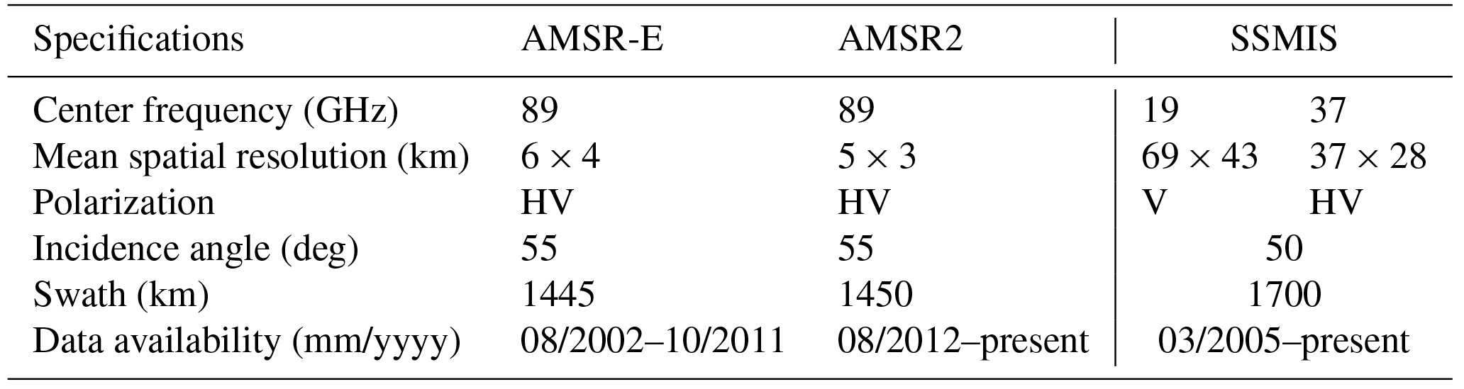
Ice concentrations derived from Advanced Microwave Scanning Radiometer (AMSR-E) of resolution 6 km ×4 km (Spreen et al., 2008) were used for the assimilation of ice concentration. AMSR-E was developed by JAXA, and it is deployed on the Aqua satellite. AMSR-E and AMSR2 are passive sensors that look at the emitted or reflected radiation from the Earth's surface with multiple frequency bands. The vertical (V) and horizontal (H) polarization channels near 89 GHz were used to compute the ice concentration from AMSR-E (Spreen et al., 2008). The Arctic Radiation and Turbulence Interaction Study (ARTIST) sea ice algorithm used to determine ice concentration from AMSR-E shows excellent results above 65 % ice concentration where the error does not exceed 10 %. With low ice concentrations, substantial deviations can occur depending on atmospheric conditions. The parameters of the sensor are provided in Table 1. AMSR-E ice concentrations were available from January 2005 to September 2011, after which the instrument stopped functioning. From August 2012 AMSR2 had been used for data collection. The same frequency (89 GHz) as that of the AMSR-E instrument was used to derive information from AMSR2. The spatial resolutions also remained the same for both AMSR-E and AMSR2. The same algorithm was applied to derive ice concentrations from both AMSR-E and AMSR2. The original AMSR-E/AMSR2 data with 6 km×4 km resolution scale were interpolated to the model grid before assimilation.
The assimilated model results of ice concentration were compared with the OSI SAF data. The details of the sensors are given in Table 1. The OSI SAF product is derived from Special Sensor Microwave Imager Sounder (SSMIS) (Bell, 2006; Tonboe et al., 2016). The data are available on a 10 km polar stereographic grid and are derived from 19 V, 37 VH channels. The erroneous data for which the ice concentration error was 100 % or the retrieval algorithm failed were filtered out before comparison. Measurements derived from AVHRR-only OISST analysis (Advanced Very High Resolution Radiometer) (Banzon et al., 2016; Reynolds et al., 2007) were used for SST assimilation. SST data products are generated using a combination of satellite and in situ observations from buoy and ship observations and are available on a resolution. The analysis product estimates SST from ice concentration only in regions where ice concentration is greater than 50 %; otherwise it uses satellite data to retrieve SST values.
Freeboard measurements from the CryoSat-2 altimeter were used to compare the freeboard estimates by the model. The CryoSat-2 altimeter operating in the SAR mode, SIRAL, has an accuracy of about 1 cm with a spatial sampling of about 45 cm (Bouzinac, 2014). The pulse-limited footprint width in the across-track direction is about 1.65 km and the beam-limited footprint width in the along-track direction is about 305 m (Scagliola, 2013), which corresponds to an along-track resolution about 401 m (assuming flat-Earth approximation). Therefore, the pulse-Doppler-limited footprint for SAR mode is about 0.6 km2. The CryoSat-2 freeboard and the ice-concentration products were generated at the Alfred Wegener Institute (AWI) (Ricker et al., 2014). The products are available in a spherical Lambert azimuthal equal-area projection of a 25 km resolution cell. The uncertainty in freeboard measurements can arise from speckle noise, lack of leads (which makes the estimation of sea surface height unreliable) and snow cover. The uncertainty up to 40 cm can be observed in the region of Baffin Bay and Labrador Sea (Ricker et al., 2014).
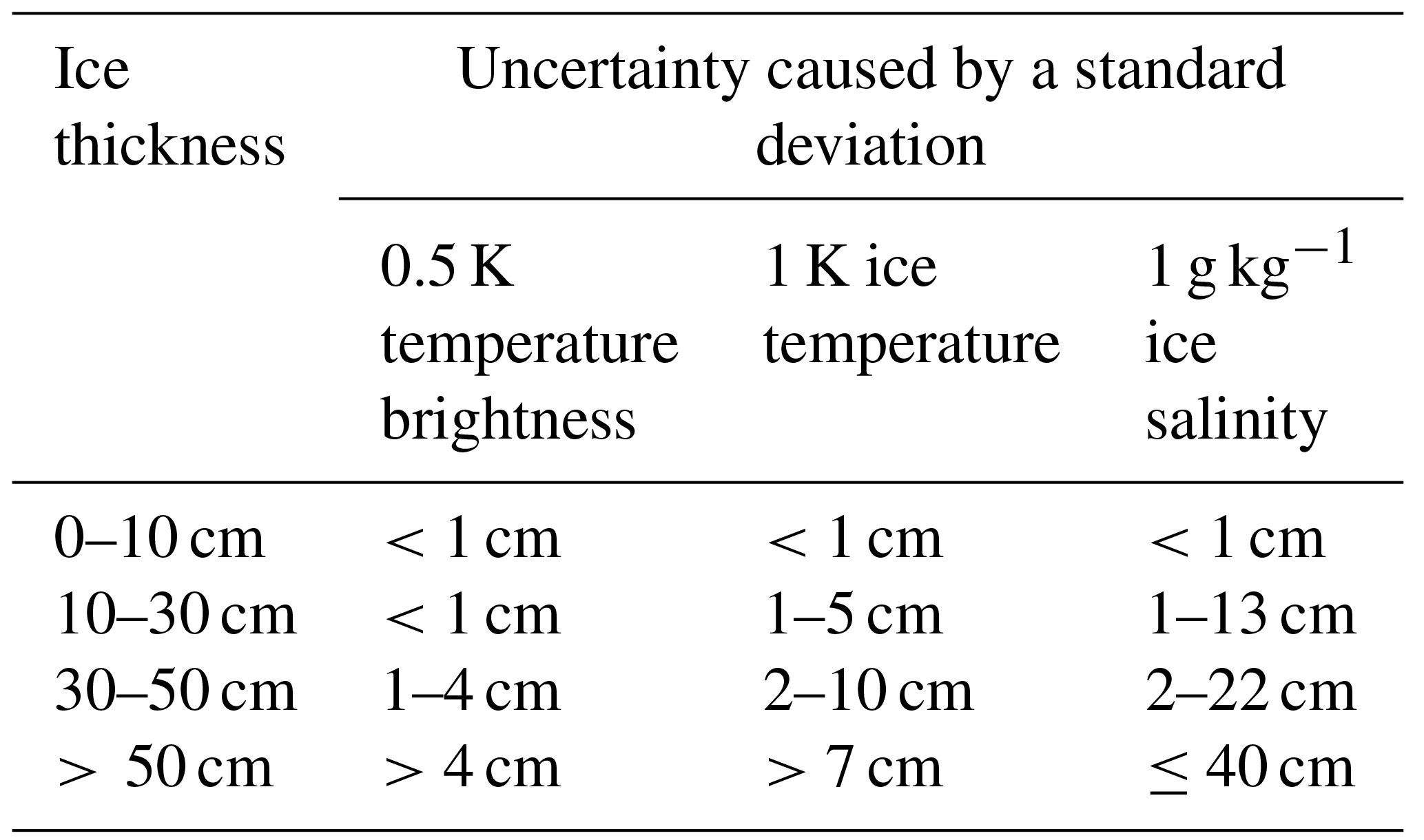
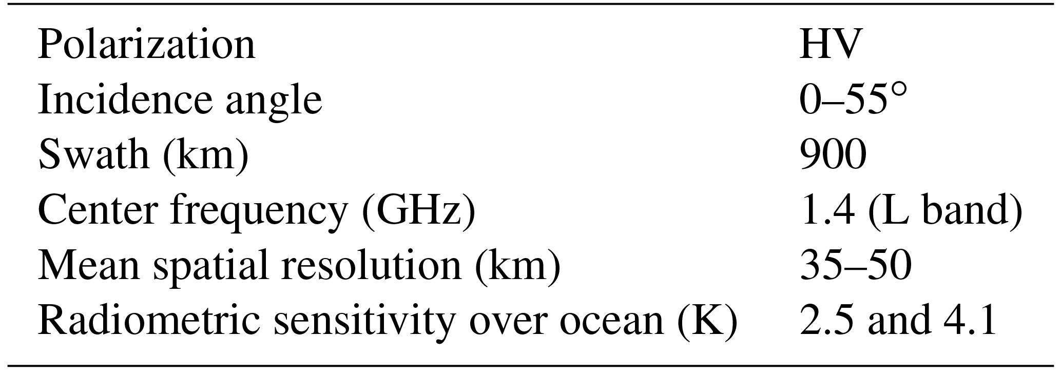
For ice thickness, the data product derived from the Soil Moisture Ocean Salinity – Microwave Imaging Radiometer using Aperture Synthesis (SMOS–MIRAS) instrument (1.4 GHz channel) (Kaleschke et al., 2012) on a grid resolution of 12.5 km×12.5 km. The ice thickness is retrieved from observation of the L-band microwave sensor of SMOS. Horizontal and vertical polarized brightness temperatures in the incidence range of are averaged. The ice thickness is then inferred from a three-layer (ocean–ice–atmosphere) dielectric slab model. SMOS data are available from 15 October 2010. The presence of snow accumulated over months can also increase the uncertainty. The uncertainty in the SMOS ice thickness (observations) shown in Table 2 (Ricker et al., 2016; Tian-Kunze et al., 2014; Tietsche et al., 2017, 2018) includes the error contributions, which are caused by the brightness temperature, ice temperature and ice salinity. The insufficient knowledge of the snow cover also introduces a large uncertainty in ice thickness estimates. Snow depth uncertainty can be 50 %–70 % of the mean value (Zhou et al., 2018). In general, the uncertainty in the thickness observation increases with increasing ice thickness, increasing snow cover and the onset of melt (Kaleschke et al., 2013). The SMOS ice thickness retrieval produces a large amount of uncertainty during the melt season and hence retrieval is not conducted during the melt season. Table 3 shows the details on the SMOS sensor (Barré et al., 2008; Kerr et al., 2001).
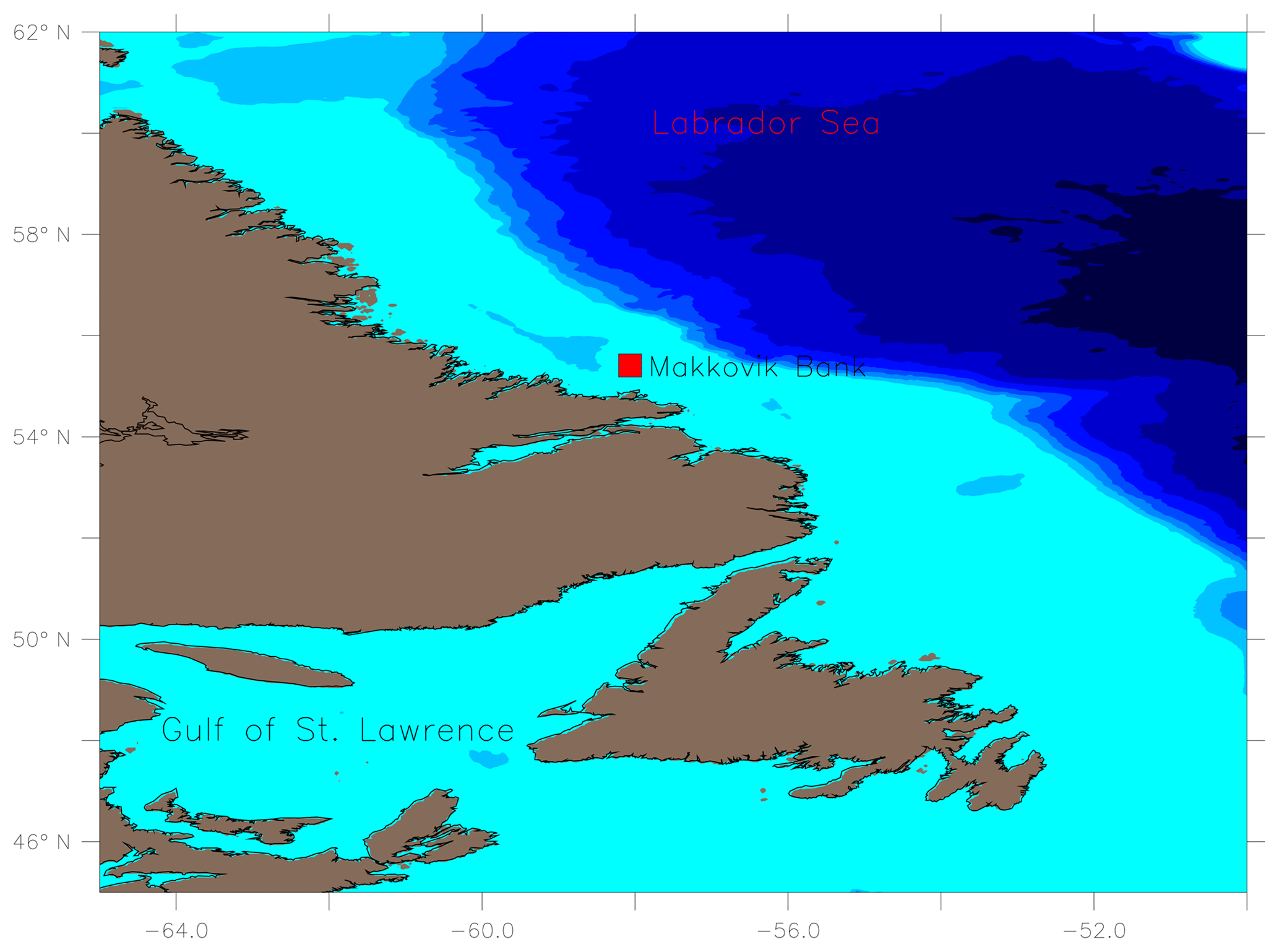
Ice draft measurements from an ULS instrument (Ross et al., 2014) located on the Makkovik Bank (see Fig. 1) at 58.0652∘ W and 55.412∘ N, were used to analyze the ridge keel and the level ice draft in the region.
The ULS data measured at an interval of approximately 5.5 s are available from the beginning of January to the end of May during 2005, 2007 and 2009. The frequency histogram of the data yields a unimodal, bimodal or multi-modal distribution. A sample histogram is provided in Fig. 2 for 10 February 2007. We assume that the first mode in the histogram corresponds to the level draft ice and the second mode corresponds to the ridge keel measurement. The first mode of the distribution is selected by finding a minimum between two peaks. The histogram was analyzed to derive daily averages of ice draft and keel measurements (Prasad et al., 2016).
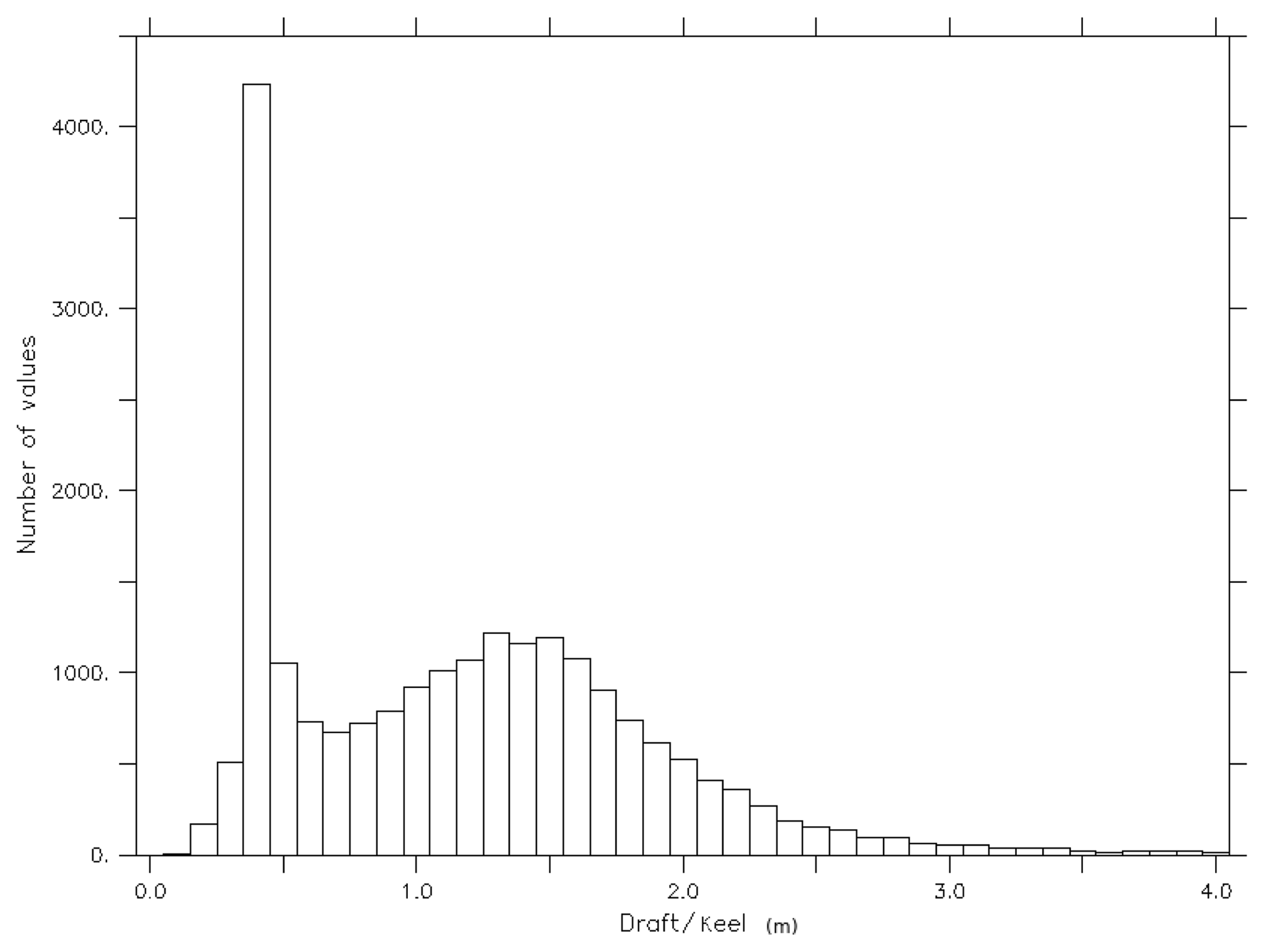
Figure 2The histogram of the ULS measurement, 10 February 2007, for the estimation of draft and keel (metres).
The assimilation module uses a combined optimal interpolation and nudging technique for ice concentration (Lindsay and Zhang, 2006; Wang et al., 2013). The method can be represented generally as Eq. (1) (Deutch, 1965; Lindsay and Zhang, 2006).
where Xa is the final analysis of the variable, Xo is the observed quantity (for ice concentration this is AMSR-E/AMSR2, for SST this is AVHRR-only OISST), Xb is the background estimate of the variable (for ice concentration and SST this is model estimate), dt is the model time step, τ is the basic nudging timescale as in Wang et al. (2013), and K is the nudging weight with the optimal interpolation value. K is computed as
where σb and σo are the error standard deviation of the model estimate (Deutch, 1965) and the observations (Deutch, 1965) respectively. The parameters in the weighing factor given in Eq. (2) are defined according to Lindsay and Zhang (2006) as ; σo=0.08 (parameter may vary spatially), α=6.
The assimilation of the ice concentration, σo=0.08, is calculated from a long-term standard deviation of 0.08, since the AMSR-E/AMSR2 ice concentration error is dependent on various atmospheric conditions for values less than 65 %. The parameter α=6 is used in the present study to ensure that the coefficients for assimilation are heavily weighted only when there is large variation between the model and the observation (Lindsay and Zhang, 2006).
SST is also assimilated using the nudging and optimal interpolation scheme. For SST assimilation, σo is fixed at 0.05 to compensate for the assumption of zero mixed-layer heat flux. A value α equal to 6 (Lindsay and Zhang, 2006) was also used for the assimilation of SST to ensure that only large differences between the model and observation are weighted heavily.
The assimilation of ice concentration is then followed by a recomputation of the estimated sea ice volume. The ice volume is subtracted or added by including the increments or decrements with specified ice thickness. Since a variable drag coefficient was used for the friction associated with an effective sea ice surface roughness at the ice–atmosphere and ice–ocean interfaces and to compute the ice to ocean heat transfer, the level ice area is updated by assuming that the model deformed ice area and volume represent the realistic values.
Three model results are discussed here: M0, the non-assimilated model; M1, the model assimilated with ice concentration from AMSR-E/AMSR2; and M2, the model assimilated with ice concentration from AMSR-E/AMSR2 and SST from AVHRR-only OISST. M2 only assimilates SST whenever there is a data gap in ice concentration from AMSR-E (e.g. from 24 March to 31 March 2005), AMSR-E data are not available and, in that case, M2 assimilates SST instead of ice in data gaps. The AMSR-E instrument stopped producing data from October 2011, and AMSR-E2 data have been used for assimilation since August 2012. The model was in spin-up for 3 months before assimilation, since it was not coupled with the ocean model. The spin-up time of 3 months is enough to estimate the ice conditions.
5.1 Ice concentration
Figure 3 column 1 shows the absolute mean difference in ice concentration between the non-assimilated model and the OSI SAF data, column 2 shows the absolute mean difference in ice concentration of the model assimilated only with ice concentration and OSI SAF data, and column 3 shows the absolute mean difference in ice concentration of the model assimilated with both ice concentration and SST and OSI SAF data. Model M2 shows improvement in the ice concentration for January and March, but little improvement between M1 and M2 for May 2010.
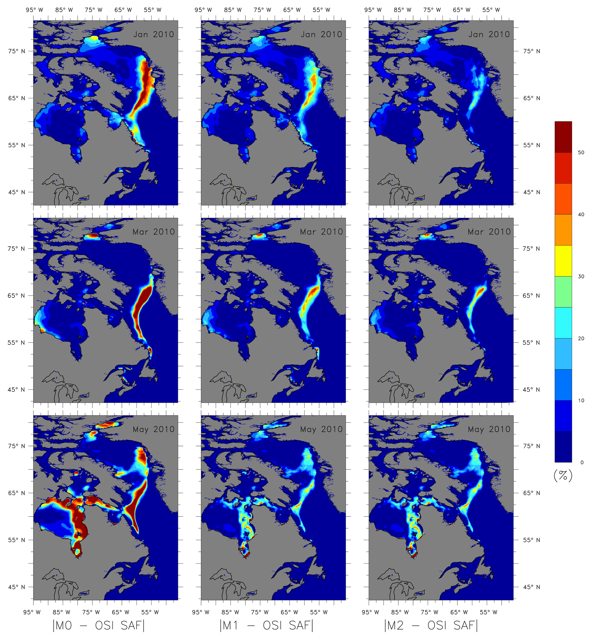
Figure 3The absolute mean difference in ice concentration from non-assimilated, assimilated models and OSI SAF data for January, March and May 2010.
Figure 4 shows the absolute mean difference in ice concentration of the model assimilated with AMSR-E/AMSR2 and OSI SAF (SSMIS) data from January 2010 to September 2011 and the absolute mean difference in ice concentration from August 2012 to December 2015. The assimilation of SST and ice concentration decreases the error between the model and the OSI SAF ice concentration. In 2010, the non-assimilated model error of 4.624 % was reduced to 1.939 % by assimilating ice concentration. The assimilation of SST and ice concentration decreased the error to about 1.118 % in 2010.

Figure 4The absolute mean difference in ice concentration for models M0, M1 and M2 is shown for January 2010 to September 2011 in row 1 and for August 2012 to December 2015 in row 2.
From October 2011 to July 2012, AMSR-E data are not available for a more extended period, and model M2 was assimilated only with SST; see Fig. 5. During this period, the SST assimilation decreases the error between the model and the observation by almost 3 %.
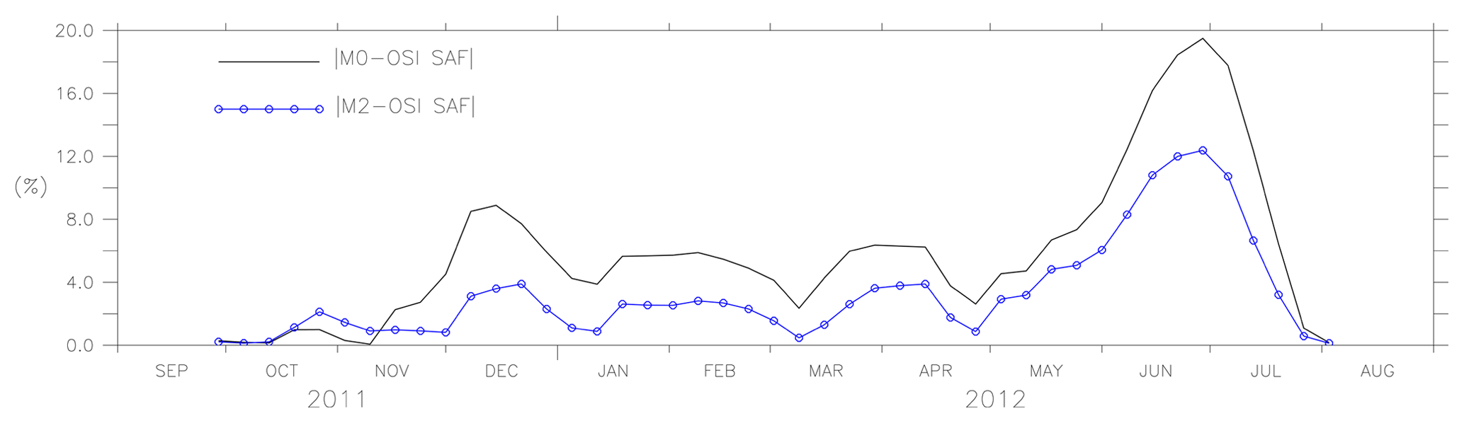
Figure 5The absolute mean difference in ice concentration from October 2011 to July 2012. Ice concentration was not available for assimilation and hence model M2 will only be assimilated with SST during this period.
5.2 Ice thickness
In this section, we compare the ice thickness from the model with that from the observation. The large unacceptable uncertainties in observation data derived from SMOS create difficulties for the analysis. Also, it is strictly recommended to not use the SMOS data with an uncertainty greater than 1 m (Tian-Kunze and Kaleschke, 2016) for practical applications. For comparison and validation, ice thickness data are selected from both the model and observation where the observed ice thickness has an uncertainty less than or equal to 100 cm. The SMOS thickness has less uncertainty for thinner ice and higher uncertainty for thicker ice; see Table 2 for the uncertainty in the SMOS ice thickness. In the case of SMOS-derived thickness, the uncertainties would increase with snow accumulation and melt onset.
Figures 6, 7 and 8 show the mean values of the thickness estimated from models M0, M1, M2 and SMOS with the uncertainty limits of the SMOS ice thickness (shaded grey). As ice thickness increases through the season, so do the uncertainty limits. The values of model M2 are within the uncertainty limits of SMOS ice thickness from October until the end of February (except for 2014). From the comparison, during March, the model results exceed the uncertainty limits. Figure 8 shows the results for the period October 2011 to April 2012 in which AMSR-E data were missing and during which M1 was not assimilated with ice concentration but used the initial conditions from the assimilated result. Model M2 used the initial conditions assimilated with both ice concentration and SST but only assimilates SST during the period. Both models, M1 and M2, show better forecasts with the improved initial conditions in the long-term analysis. One of the reasons why the model values exceed the uncertainty limits during March is the choice of α=6, which considers only large differences while weighing the coefficient K. Since the assimilation shows improvement in ice thickness, using a value of α=2, it is expected to impose the model values within the uncertainty limits.
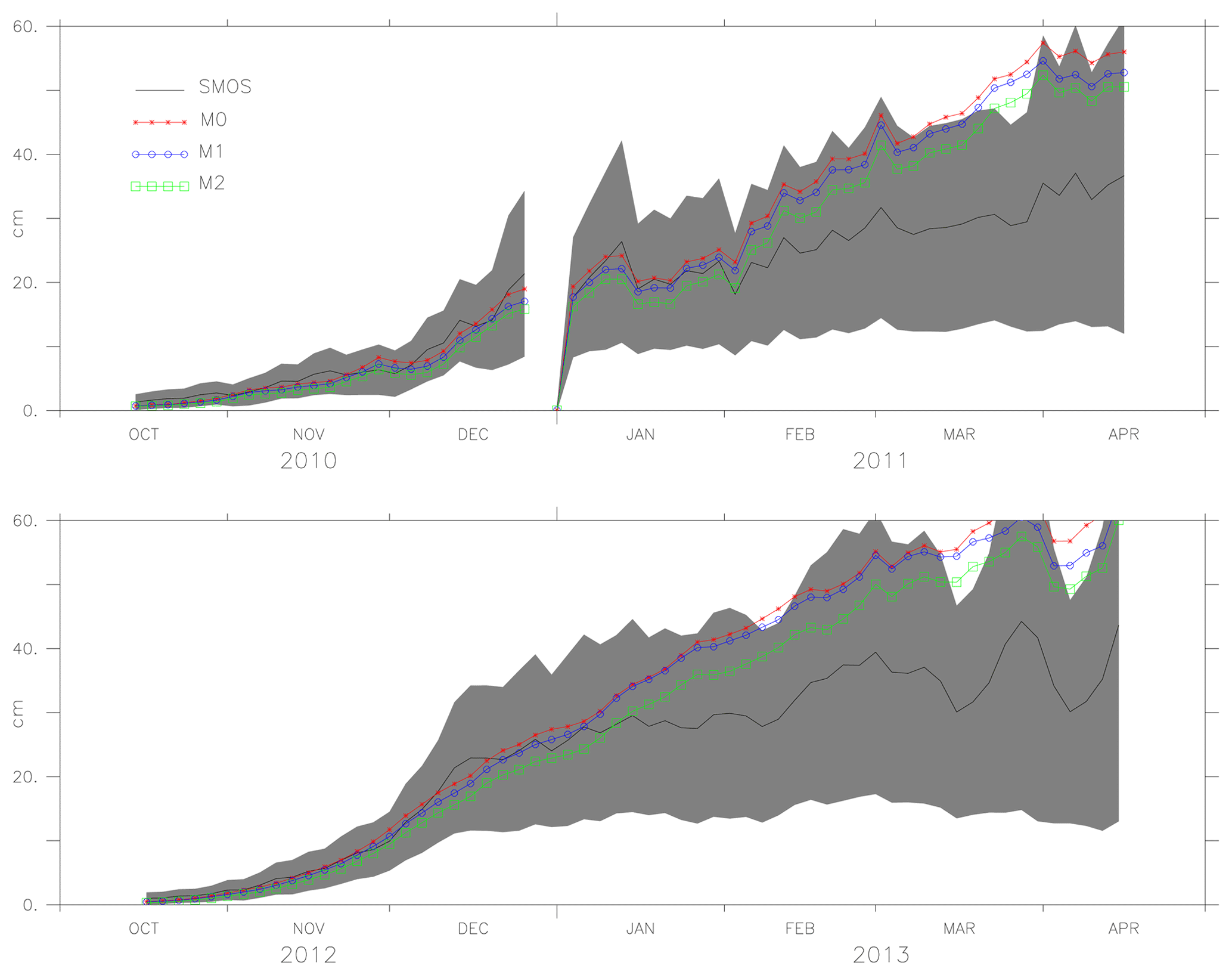
Figure 6The ice thickness from the models M0, M1, M2 and observation (SMOS ice thickness) from October 2010 to April 2011 and October 2012 to April 2013. The uncertainty in the observation (SMOS ice thickness) is shaded in grey.
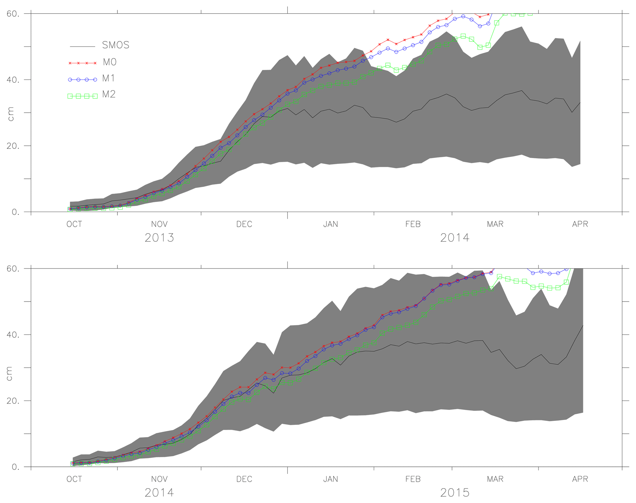
Figure 7The ice thickness from the models M0, M1, M2 and observation (SMOS ice thickness) from October 2013 to April 2014 and October 2014 to April 2015. The uncertainty in the observation (SMOS ice thickness) is shaded in grey.
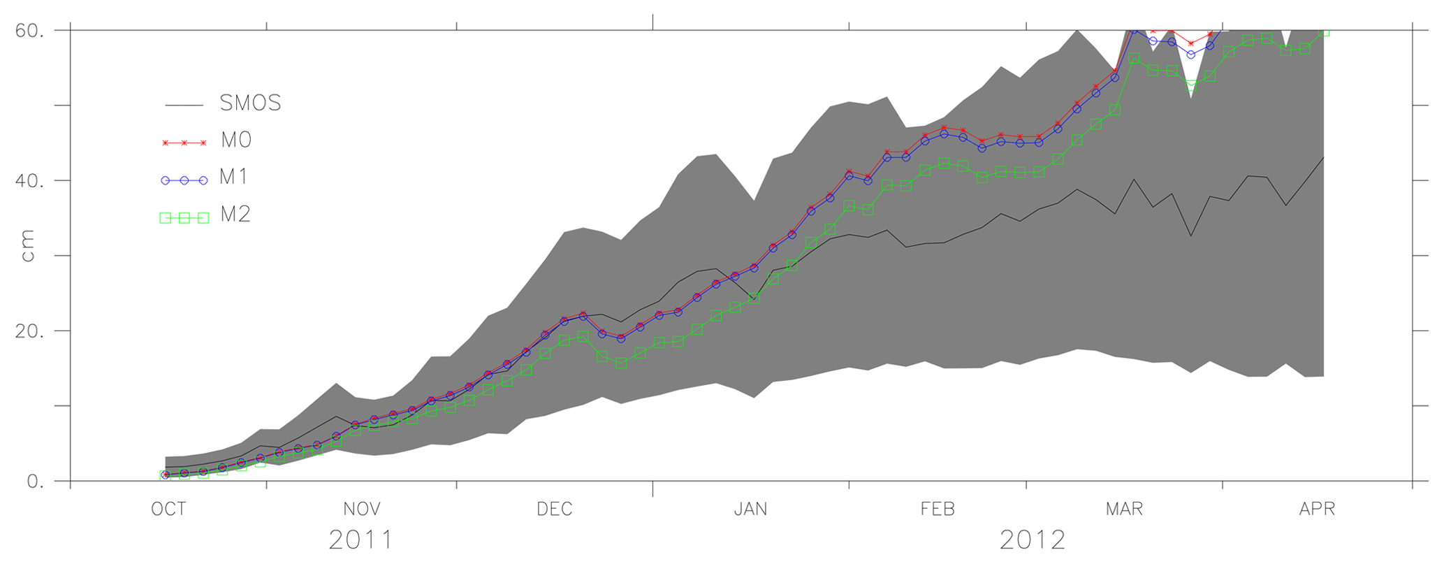
Figure 8The ice thickness from models M0, M1 (ice concentration was not assimilated as there were no AMSR-E data available, but the initial conditions from the model assimilated with ice concentration were used), M2 (assimilated only with SST and used model initial conditions derived from assimilating both ice concentration and SST) and observations (SMOS ice thickness) from October 2011 to April 2012. The uncertainty in the observation (SMOS ice thickness) is shaded in grey.
The model M2 thickness, SMOS-derived ice thickness and the uncertainty in the SMOS-derived measurement for 15 December 2010, 15 January 2011 and 15 March 2011 are shown in Fig. 9, which includes regions where observed uncertainties are larger than 1 m.
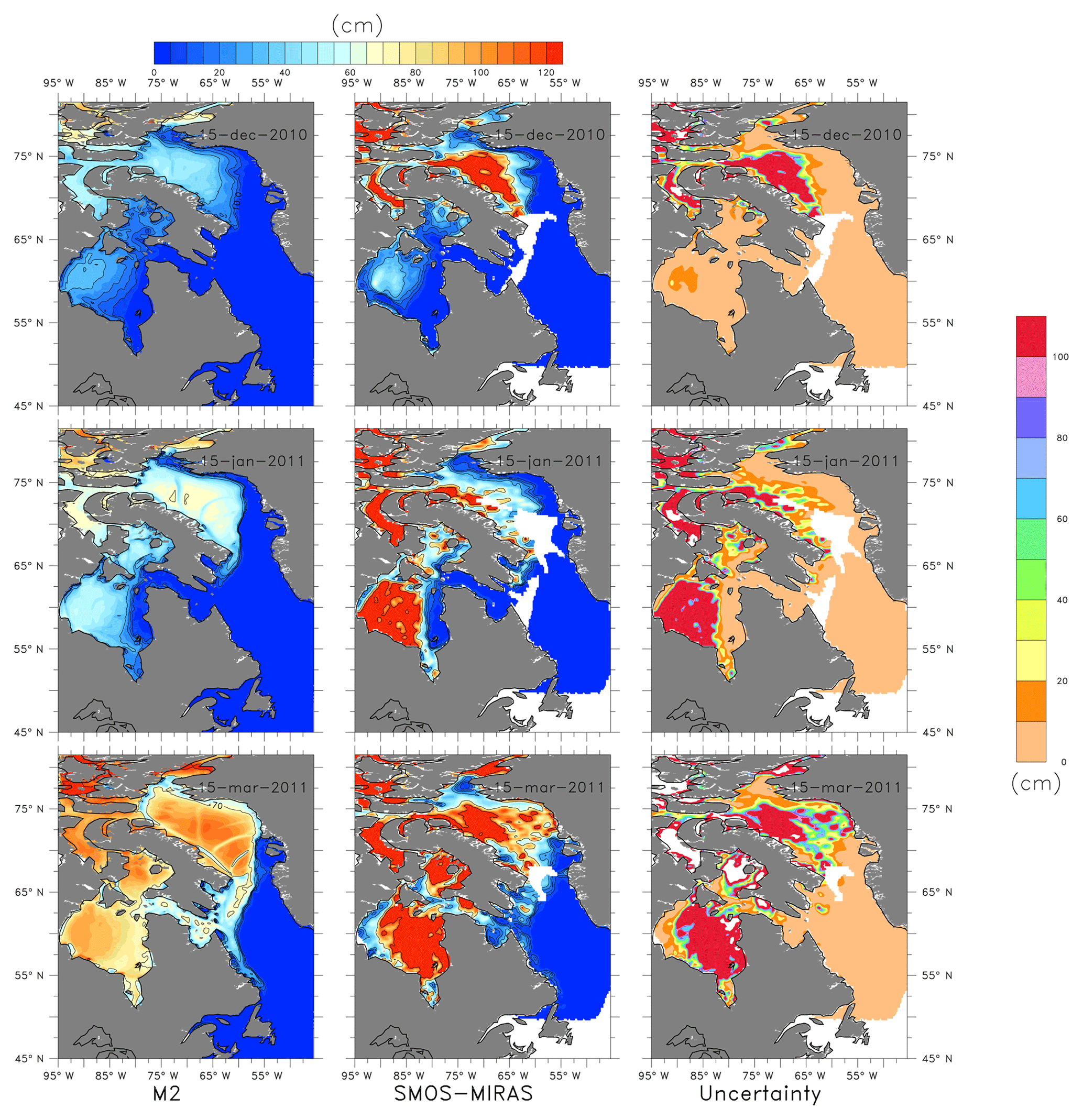
Figure 9The M2-estimated ice thickness, SMOS–MIRAS-derived ice thickness and the observation uncertainty for 15 December 2010, 15 January and 15 March 2011.
The thickness results for thin ice categories (<30 cm) from the model with SMOS are shown in Figs. 10, 11 and 12. The shaded region shows the uncertainty in the thin ice from SMOS data. The thin ice category thicknesses are overestimated from October to the end of November but the values are within the uncertainty limits of SMOS from December to March.
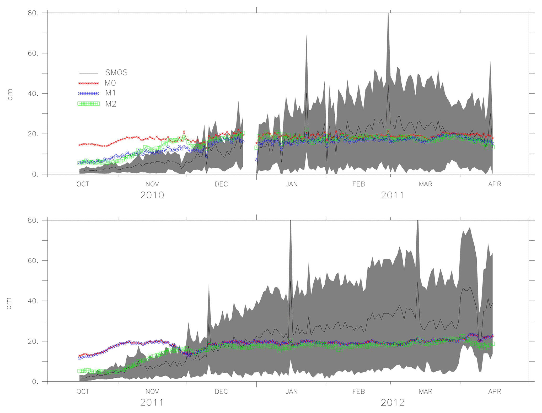
Figure 10The ice thickness from the models M0, M1, M2 and observation (SMOS ice thickness) and the observation uncertainty (shaded grey) for SMOS ice thickness less than 30 cm (2010–2012).
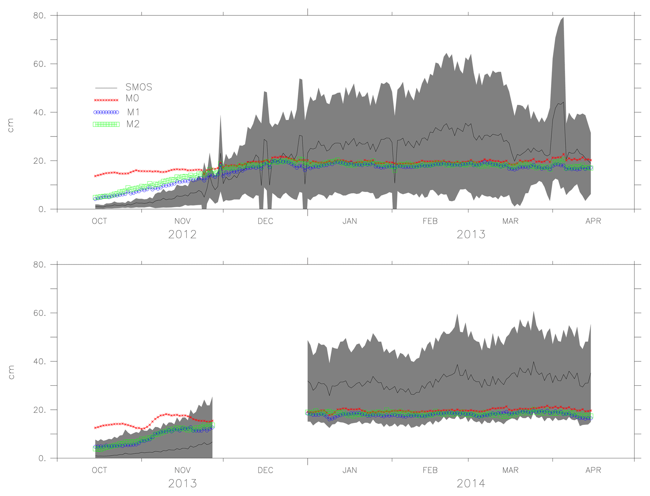
Figure 11The ice thickness from the models M0, M1, M2 and observation (SMOS ice thickness) and the observation uncertainty (shaded grey) for SMOS ice thickness less than 30 cm (2012–2014).

Figure 12The ice thickness from the models M0, M1, M2 and observation (SMOS ice thickness) and the observation uncertainty (shaded grey) for SMOS ice thickness less than 30 cm (2014–2015).
Figure 13 shows the SST from AVHRR-only OISST analysis with the shaded regions representing the observation uncertainty and SST from models M0, M1 and M2. In general, the SST from AVHRR-only OISST assimilation improves the ice concentration and ice thickness results for the model M2. The assimilated model M2 still has a systematic bias during the summer and winter, which may be improved by decreasing α (=6, presently) and by decreasing the nudging timescale (presently for SST, the nudging scale is 30 days). Decreasing the nudging timescale can result in the late formation and early melt of ice (not shown here). The results can be improved by making the nudging timescale less frequent during the formation and more frequent during the winter, until the beginning or middle of March. Frequent nudging is also found to produce blow-up for the thermodynamic model. The parameters in the assimilation have to be selected to maintain balance, not cause late formation and earlier melt and maintain the stability of the model thermodynamics and dynamics. For M0, the non-assimilated model, the results may be improved by including the mixed-layer heat flux in a parameterization similar to Petty et al. (2014). Also, note that the model still assumes a fixed salinity profile and mixed-layer profile.
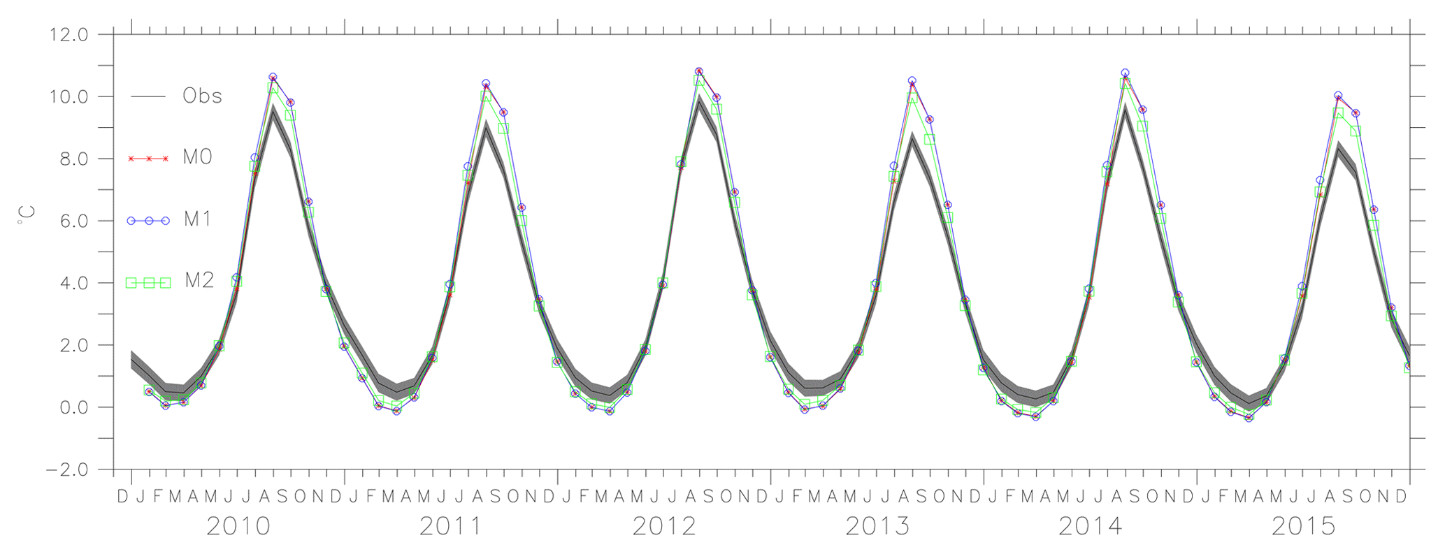
Figure 13The SST from AVHRR-only OISST analysis with the shaded region represents the uncertainty in AVHRR-only OISST analysis and SST from models M0, M1 and M2.
5.3 Draft and keel depth
The ULS measurements were separated into level ice draft and keel depth measurement as described in Prasad et al. (2016) and also in Sect. 3. The level ice draft, D, is computed using Eq. (3) (Tsamados et al., 2014). The results are shown in Fig. 14.
where ρi=917 kg m−3 is the density of ice, vice is the volume of ice, ρs=330.0 kg m−3 is the density of snow, vsno is the volume of snow, A is ice concentration, and ρw=1026 kg m−3 is the density of seawater.
Some deviations are noticed in the comparison of level ice draft. The estimated absolute error is about 10 cm for 2005, 2007 and 2009. The error of 10 cm on a draft of 20 cm can be accepted considering large differences in spatial resolution between the ULS and model. Also, the analysis was done only for 2005, 2007 and 2009 as this was when data were available. The discrepancy occurs due to the fact that ULS gives values at a particular location with high resolution (within the footprint of several metres), while the model of 10 km resolution gives an averaged result close to the location of the ULS. Moreover, the analysis of the histogram from ULS shows a multi-modal distribution at certain time points which indicates the presence of rafted ice. In the present study, the rafted ice is also included and considered as the ridges which contribute towards the results achieved in this section.
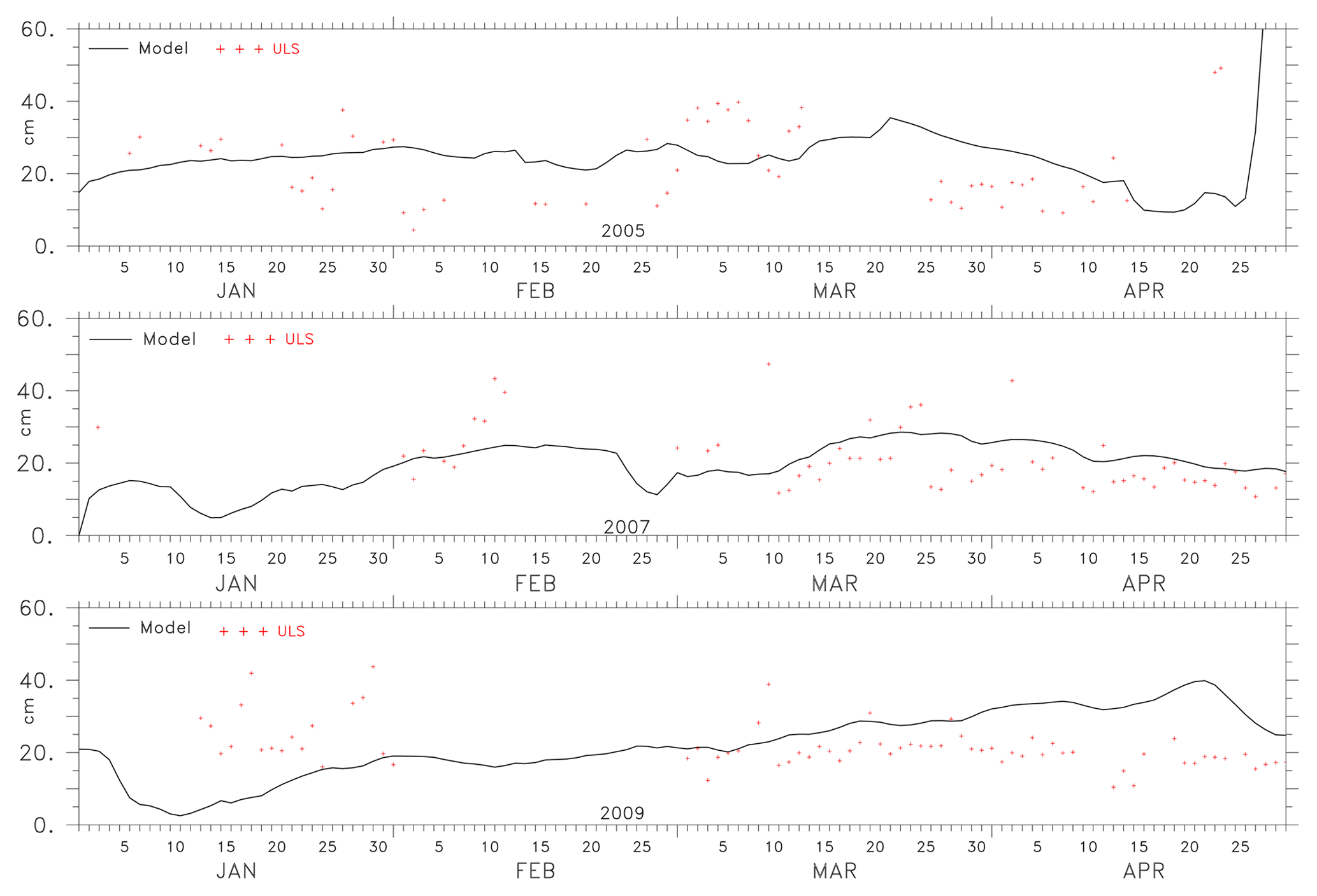
Figure 14The level ice draft computed from the ULS measurement and the M2 model-estimated values at Makkovik Bank for 2005, 2007 and 2009.
The keel is computed using idealized sea ice floe comprising a system of two triangular sails and keels and a single melt pond (Tsamados et al., 2014). The ridge height is given by Eq. (4) and the correlation between the ridge height and keel depth is given by Eq. (5):
where Hr is the ridge height, ; is the slope of the sail and ; is the slope of the keel; ϕr is the porosity of the ridges; (Shokr and Sinha, 2015) is the porosity of the keels. Dk=5 is the ratio distance between ridge and distance between the keels. Vrdg is the volume of the ridged ice, Ardg is the ridged ice area fraction, α and β are the weight functions for area of ridged ice, C is the coefficient that relates ridge to keel, and
gives the keel depth Hk. The Makkovik Bank where the keel measurements are estimated from ULS has high variability of ice thickness, and frequency of the formation of keels is high due to the combined effect of the Labrador currents and winds. Rafted ice is common in this region (Peterson et al., 2013). Here the model and the observation of keel depth are used to estimate the parameter C.
The coefficient C, estimated for 2005, 2007 and 2009, shows that a value between 3.00 and 4.50 gives a good estimate of keel measurement for January and February, while a value between 7.00 and 8.00 gives a good estimate of keel during March, April and May. In Fig. 15 the values of the coefficient C that relates ridge to keel for January and February is 3 and C=7.00 for March, April and May; see Eq. (5). These values are derived under the assumptions in Eq. (4). The sensitivity of parameters has to be further explored to determine the characteristics of each parameter and its effect on the ridge–keel relationship, which may result in a different conclusion. Since the interest lies in deriving this relationship from the assimilated model, only results from M2 is presented. For non-assimilated models, the choice of parameters vary.
During January to February the formation of ice and ridges occurs, and during March the thick ice may be contributing towards the ridging, thus increasing the value of C.
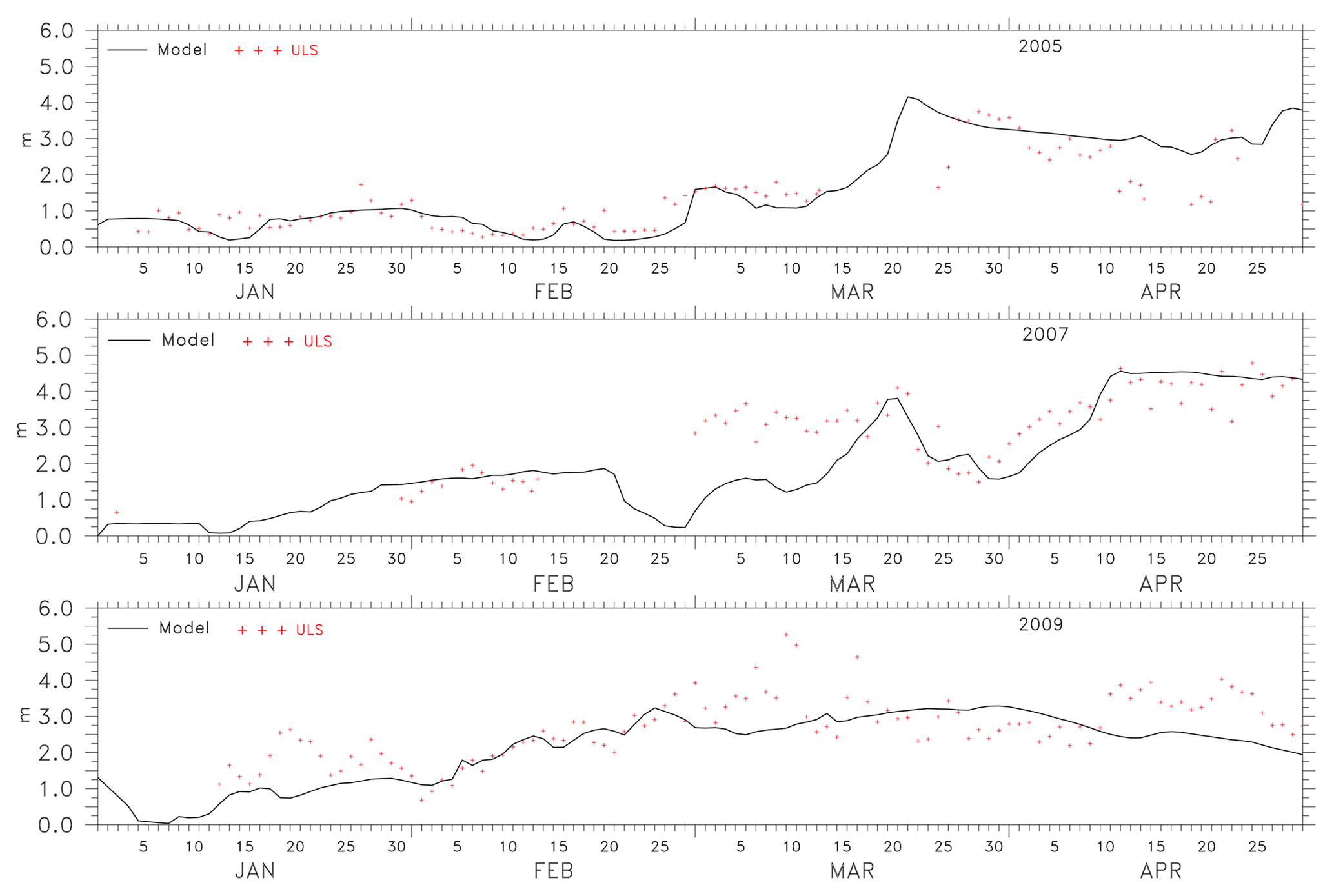
Figure 15The keel depth computed from the ULS measurement and the M2-estimated values in centimetres for 2005, 2007 and 2009.
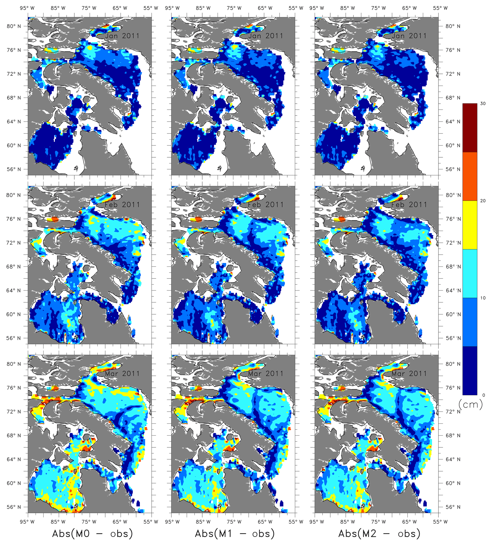
Figure 16The absolute mean difference between the model freeboard for M0, M1 and M2 and CryoSat-2 for January, February and March 2011.
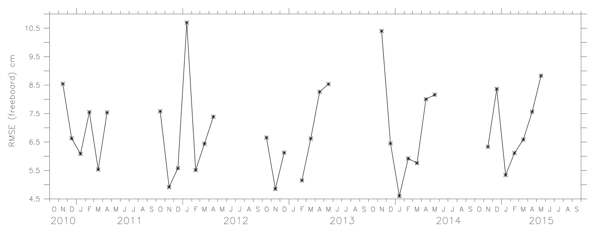
Figure 17The RMSE of freeboard measure for the regions where the lead fraction is above 0 %.

Figure 18The freeboard from model M2, CryoSat-2 and the uncertainty in the observations for January, February and March 2011.
5.4 Freeboard
The uncertainty in freeboard measurements can arise due to the lack of leads. The presence of leads was ensured by selecting the regions where the lead fraction derived from CryoSat-2 (Ricker et al., 2014) was greater than zero. In the model, freeboard is computed using Eq. (6) (Tsamados et al., 2014). For the region, the uncertainty in the freeboard measurements is below 40 cm (Ricker et al., 2014).
where vice is the volume of ice, vsno is the volume of snow, A is the ice concentration and D is the draft; see Eq. (3).
The absolute mean difference between the model and the observations for January, February and March 2011 is shown in Fig. 16. M2 freeboard measurements are close to the observed freeboard. Figure 17 shows the RMSE of the freeboard from model M2 and CryoSat-2 in the areas where the lead fraction was greater than zero. The RMSE is below the maximum uncertainty in 40 cm for the region of interest and was found to range between 4.5 and 11 cm.
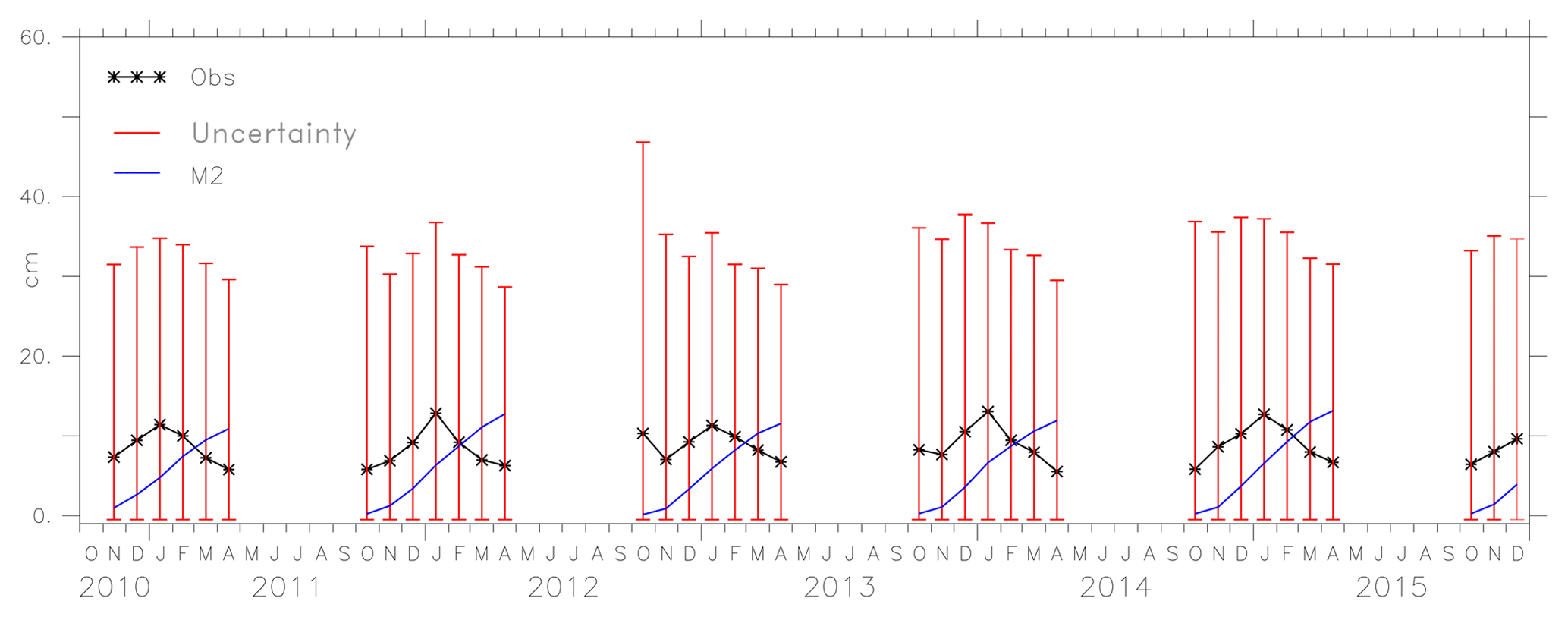
Figure 18 shows the observed freeboard from CryoSat-2, the uncertainty in the observation and the model M2. Only the model results from M2 are given, since there are only slight deviations for M0 and M1 from the observation. Moreover, we are interested in the results of the assimilated model and how well it performs in the estimation of freeboard. The model values are within the uncertainty limits of the observation. Also, note that the model results are monthly averaged, while CryoSat-2 is a mosaic of daily measurements within a month. The spatial average of freeboard for the region, the observed value and the uncertainty are shown in Fig. 19. The average freeboard from the model lies within the uncertainty limits of the observation.
The assimilated models in the literature and those implemented in forecasting centres use a constant drag formulation and lack details on deriving parameters other than ice concentration and ice thickness (Lemieux et al., 2016; Rae et al., 2015). In this work a variable drag formulation is used for the friction associated with an effective sea ice surface roughness at the ice–atmosphere and ice–ocean interfaces and to compute the ice-to-ocean heat transfer. The results from the updated model were compared with satellite-derived measurements to validate the model estimates of ice concentration, ice thickness and freeboard. Moreover, the model results were used to estimate the relationship between sail and keel depth.
The modelled ice thickness demonstrated a good correspondence with the estimates from SMOS–MIRAS, except during the period of maximum ice extent. The deviation in the results of ice thickness during March have to be further explored by tuning the parameters that contribute to the ice thickness in the non-assimilated model as well as the assimilation parameters. The thin ice category thicknesses are overestimated from October to the end of November but the values are within the uncertainty limits of SMOS from December to March. The SMOS estimates are influenced by the presence of snow, and also, during the melt seasons the uncertainties of SMOS-estimated ice thickness might increase, in which case comparison with more reliable data would be required. The model freeboard are compared with estimates from CryoSat-2, and the RMSE was found to range between 4.5 and 11 cm. The estimates of freeboard from the model are within the uncertainty values of the CryoSat-2 (below 40 cm).
The level ice draft and keel values derived from ULS were compared with the modelled values. The coefficient that related the sail height and keel depth for the Makkovick region lies in the range 3–8 depending on the period of the year. Since the variable drag formulation depends on the assimilation methodology, further sensitivity studies have to be conducted for the optimization of the model. The model will be made operational after further sensitivity studies.
Data used for this paper are freely available.
The first author performed the simulation and contributed to writing the paper. All co-authors participated in the discussions and contributed to writing and editing the paper.
The authors declare that they have no conflict of interest.
Funding support was provided by the Research and Development Corporation (RDC),
Newfoundland and Labrador. The authors also thank Tony King (C-CORE) and
Ingrid Peterson (DFO, Government of Canada) for providing ULS data from
Makkovik Bank. We also thank the Center for Health Informatics and Analytics
(CHIA), MUN and ACENet, Canada for providing computational resources. We
would like to thank the developers of CICE, the Los Alamos sea ice model for
public availability of the sea ice model and the users' group. The authors
would like to acknowledge the anonymous referees and editor for their fruitful
comments and suggestions.
Edited by: John Yackel
Reviewed by: two anonymous referees
Banzon, V., Smith, T. M., Chin, T. M., Liu, C., and Hankins, W.: A long-term record of blended satellite and in situ sea-surface temperature for climate monitoring, modeling and environmental studies, Earth Syst. Sci. Data, 8, 165–176, https://doi.org/10.5194/essd-8-165-2016, 2016. a
Barré, H. M., Duesmann, B., and Kerr, Y. H.: SMOS: The mission and the system, IEEE T. Geosci. Remote, 46, 587–593, 2008. a
Bell, W.: A preprocessor for SSMIS radiances scientific description, Met Office, UK, 2006. a
Bouzinac, C.: CryoSat product handbook, ESA User Manual, ESA, ESRIN, Italy, 2014. a
Carsey, F. D.: Microwave remote sensing of sea ice, American Geophysical Union, 1992. a
Caya, A., Buehner, M., Shokr, M., and Carrieres, T.: A first attempt of data assimilation for operational sea ice monitoring in Canada, in: 2006 IEEE International Symposium on Geoscience and Remote Sensing, IGARSS 2006, Denver, CO, USA, 31 July–4 August 2006, IEEE, 1705–1708, 2006. a, b, c, d
Caya, A., Buehner, M., and Carrieres, T.: Analysis and forecasting of sea ice conditions with three-dimensional variational data assimilation and a coupled ice–ocean model, J. Atmos. Ocean. Tech., 27, 353–369, 2010. a, b, c
Deutch, R.: Estimation theory, Prentice-Hall, Upper Sadddle River, NJ, 1965. a, b, c
Dzierzbicka-Głowacka, L., Janecki, M., Nowicki, A., and Jakacki, J.: Activation of the operational ecohydrodynamic model (3D CEMBS) – the ecosystem module, Oceanologia, 55, 543–572, 2013. a
Fenty, I. and Heimbach, P.: Coupled sea ice–ocean-state estimation in the Labrador Sea and Baffin Bay, J. Phys. Oceanogr., 43, 884–904, 2013. a
Hunke, E. C., Lipscomb, W. H., Turner, A. K., Jeffery, N., and Elliott, S.: CICE: the Los Alamos Sea Ice Model Documentation and Software User's Manual Version 5.1 LA-CC-06-012, T-3 Fluid Dynamics Group, Los Alamos National Laboratory, 75 pp., 2015. a, b
Kaleschke, L., Tian-Kunze, X., Maaß, N., Mäkynen, M., and Drusch, M.: Sea ice thickness retrieval from SMOS brightness temperatures during the Arctic freeze-up period, Geophys. Res. Lett., 39, L05501, https://doi.org/10.1029/2012GL050916, 2012. a
Kaleschke, L., Tian-Kunze, X., Maaß, N., Heygster, G., Huntemann, M., Wang, H., and Haas, C.: SMOS Sea Ice Retrieval Study (SMOSIce), ESA Support To Science Element (STSE), Final Report ESA ESTEC, Tech. rep., 4000101476/10/NL/CT, 2013. a
Karvonen, J., Cheng, B., Vihma, T., Arkett, M., and Carrieres, T.: A method for sea ice thickness and concentration analysis based on SAR data and a thermodynamic model, The Cryosphere, 6, 1507–1526, https://doi.org/10.5194/tc-6-1507-2012, 2012. a
Kerr, Y. H., Waldteufel, P., Wigneron, J.-P., Martinuzzi, J., Font, J., and Berger, M.: Soil moisture retrieval from space: The Soil Moisture and Ocean Salinity (SMOS) mission, IEEE T. Geosci. Remote, 39, 1729–1735, 2001. a
Kubat, I., Sayed, M., Savage, S. B., and Carrieres, T.: Numerical simulations of ice thickness redistribution in the Gulf of St. Lawrence, Cold Reg. Sci. Technol., 60, 15–28, 2010. a
Lemieux, J.-F., Beaudoin, C., Dupont, F., Roy, F., Smith, G. C., Shlyaeva, A., Buehner, M., Caya, A., Chen, J., Carrieres, T., Pogson, L., DeRepentigny, P., Plante, A., Pestieau, P., Pellerin, P., Ritchie, H., Garric, G., and Ferry, N.: The Regional Ice Prediction System (RIPS): verification of forecast sea ice concentration, Q. J. Roy. Meteor. Soc., 142, 632–643, 2016. a, b, c
Levitus, S. and Mishonov, A.: The world ocean database, Data Science Journal, 12, WDS229–WDS234, 2013. a
Lindsay, R. and Zhang, J.: Assimilation of ice concentration in an ice–ocean model, J. Atmos. Ocean. Tech., 23, 742–749, 2006. a, b, c, d, e, f, g
Mesinger, F., DiMego, G., Kalnay, E., Mitchell, K., Shafran, P. C., Ebisuzaki, W., Jović, D., Woollen, J., Rogers, E., Berbery, E. H., et al.: North American regional reanalysis, B. Am. Meteorol. Soc., 87, 343–360, 2006. a
Peterson, I. K., Prinsenberg, S. J., and Belliveau, D.: Sea-ice draft and velocities from moorings on the Labrador Shelf (Makkovik Bank): 2003–2011, Canadian Technical Report of Hydrography and Ocean Sciences 281, available at: http://waves-vagues.dfo-mpo.gc.ca/Library/348086.pdf (last access: 5 December 2018), 2013. a
Petty, A. A., Holland, P. R., and Feltham, D. L.: Sea ice and the ocean mixed layer over the Antarctic shelf seas, The Cryosphere, 8, 761–783, https://doi.org/10.5194/tc-8-761-2014, 2014. a
Prasad, S., Zakharov, I., Bobby, P., and McGuire, P.: The implementation of sea ice model on a regional high-resolution scale, Ocean Dynam., 65, 1353–1366, 2015. a, b, c, d, e
Prasad, S., Zakharov, I., Bobby, P., Power, D., McGuire, P., et al.: Model Based Estimation of Sea Ice Parameters, in: Arctic Technology Conference, Offshore Technology Conference, St. John's, NL, Canada, 24–26 October 2016. a, b
Rae, J. G. L., Hewitt, H. T., Keen, A. B., Ridley, J. K., West, A. E., Harris, C. M., Hunke, E. C., and Walters, D. N.: Development of the Global Sea Ice 6.0 CICE configuration for the Met Office Global Coupled model, Geosci. Model Dev., 8, 2221–2230, https://doi.org/10.5194/gmd-8-2221-2015, 2015. a
Reynolds, R. W., Smith, T. M., Liu, C., Chelton, D. B., Casey, K. S., and Schlax, M. G.: Daily high-resolution-blended analyses for sea surface temperature, J. Climate, 20, 5473–5496, 2007. a
Ricker, R., Hendricks, S., Helm, V., Skourup, H., and Davidson, M.: Sensitivity of CryoSat-2 Arctic sea-ice freeboard and thickness on radar-waveform interpretation, The Cryosphere, 8, 1607–1622, https://doi.org/10.5194/tc-8-1607-2014, 2014. a, b, c, d
Ricker, R., Hendricks, S., Kaleschke, L., and Tian-Kunze, X.: CS2SMOS: Weekly Arctic Sea-Ice Thickness Data Record, User Guide, available at: http://epic.awi.de/41602/ (last access: 5 December 2018), 2016. a
Ross, E., Fissel, D., Wyatt, G., Milutinovic, N., and Lawrence, J.: Project report: Data processing and analysis of the ice draft and ice velocity, Makkovik Bank, Project Report for Bedford Institute of Oceanography, Dartmouth, NS, Canada by ASL Environmental Sciences Inc., Victoria, B.C. Canada, 19 pp., 2014. a
Sayed, M. and Carrieres, T.: Overview of a new operational ice model, in: The Ninth International Offshore and Polar Engineering Conference, International Society of Offshore and Polar Engineers, Brest, France, 30 May–4 June 1999. a, b
Sayed, M., Savage, S., and Carrieres, T.: Examination of Ice Ridging Methods Using Discrete Particles, in: Proceedings 16th International Conference on Port and Ocean Engineering under Arctic Conditions (POAC'01), 12–17 August 2001, Ottawa, Ontario, Canada, 1087–1096, 2001. a
Sayed, M., Carrieres, T., Tran, H., and Savage, S. B.: Development of an operational ice dynamics model for the Canadian Ice Service, in: The Twelfth International Offshore and Polar Engineering Conference, International Society of Offshore and Polar Engineers, Kitakyushu, Japan, 26–31 May 2002. a, b
Scagliola, M.: CryoSat footprints Aresys technical note, SAR-CRY2-TEN-6331, Aresys/ESA, Italy, 2013. a
Shokr, M. and Sinha, N.: Sea ice: physics and remote sensing, John Wiley & Sons, American Geophysical Union, USA, 2015. a
Spreen, G., Kaleschke, L., and Heygster, G.: Sea ice remote sensing using AMSR-E 89-GHz channels, J. Geophys. Res., 113, C02S03, https://doi.org/10.1029/2005JC003384, 2008. a, b
Stirling, I.: The biological importance of polynyas in the Canadian Arctic, Arctic, 33, 303–315, 1980. a
Tian-Kunze, X. and Kaleschke, L.: Read-me-first note for the release of the SMOS Level 3 ice thickness data product, Technical Note, University of Hamburg, Germany, 2016. a
Tian-Kunze, X., Kaleschke, L., Maaß, N., Mäkynen, M., Serra, N., Drusch, M., and Krumpen, T.: SMOS-derived thin sea ice thickness: algorithm baseline, product specifications and initial verification, The Cryosphere, 8, 997–1018, https://doi.org/10.5194/tc-8-997-2014, 2014. a
Tietsche, S., Balmaseda, M., Zuo, H., and de Rosnay, P.: Comparing Arctic Winter Sea-ice Thickness from SMOS and ORAS5, European Centre for Medium-Range Weather Forecasts, European Centre for Medium-Range Weather Forecasts, Reading, England, 2017. a
Tietsche, S., Alonso-Balmaseda, M., Rosnay, P., Zuo, H., Tian-Kunze, X., and Kaleschke, L.: Thin Arctic sea ice in L-band observations and an ocean reanalysis, The Cryosphere, 12, 2051–2072, https://doi.org/10.5194/tc-12-2051-2018, 2018. a
Tonboe, R., Lavelle, J., Pfeiffer, R.-H., and Howe, E.: Product User Manual for OSI SAF Global Sea Ice Concentration, Danish Meteorological Institute, Denmark, 2016. a
Tsamados, M., Feltham, D. L., Schroeder, D., Flocco, D., Farrell, S. L., Kurtz, N., Laxon, S. W., and Bacon, S.: Impact of variable atmospheric and oceanic form drag on simulations of Arctic sea ice, J. Phys. Oceanogr., 44, 1329–1353, 2014. a, b, c
Wang, K., Debernard, J., Sperrevik, A. K., Isachsen, P. E., and Lavergne, T.: A combined optimal interpolation and nudging scheme to assimilate OSISAF sea-ice concentration into ROMS, Ann. Glaciol., 54, 8–12, 2013. a, b, c, d, e
Zhou, L., Xu, S., Liu, J., and Wang, B.: On the retrieval of sea ice thickness and snow depth using concurrent laser altimetry and L-band remote sensing data, The Cryosphere, 12, 993–1012, https://doi.org/10.5194/tc-12-993-2018, 2018. a