A simulation of a large-scale drifting snowstorm in the turbulent boundary layer

Drifting snowstorms are an important aeolian process that reshape alpine glaciers and polar ice shelves, and they may also affect the climate system and hydrological cycle since flying snow particles exchange considerable mass and energy with air flow. Prior studies have rarely considered full-scale drifting snowstorms in the turbulent boundary layer; thus, the transportation feature of snow flow higher in the air and its contribution are largely unknown. In this study, a large-eddy simulation is combined with a subgrid-scale velocity model to simulate the atmospheric turbulent boundary layer, and a Lagrangian particle tracking method is adopted to track the trajectories of snow particles. A drifting snowstorm that is hundreds of meters in depth and exhibits obvious spatial structures is produced. The snow transport flux profile at high altitude, previously not observed, is quite different from that near the surface; thus, the extrapolated transport flux profile may largely underestimate the total transport flux. At the same time, the development of a drifting snowstorm involves three typical stages, rapid growth, gentle growth, and equilibrium, in which large-scale updrafts and subgrid-scale fluctuating velocities basically dominate the first and second stages, respectively. This research provides an effective way to gain an insight into natural drifting snowstorms.

1 Introduction

Snow, one type of solid precipitation, is an important source of material to mountain glaciers and polar ice sheets, which are widespread throughout high and cold regions (Chang et al., 2016; Gordon and Taylor, 2009; Lehning et al., 2008). A common natural phenomenon over snow cover is the drifting snowstorm, which occurs when the wind speed exceeds a critical value (Doorschot et al., 2004; Li and Pomeroy, 1997; Sturm and Stuefer, 2013). Drifting snow can entrain loose snow particles on the bed into the air, which may be further transported to high altitude by turbulent eddies (King, 1990; Mann et al., 2000; Nemoto and Nishimura, 2004). Drifting snow clouds can typically range in thickness from tens to thousands of meters (Mahesh et al., 2003; Palm et al., 2011), which may not only affect people's daily life by reducing the visibility and producing local accumulation (Gordon and Taylor, 2009; Mohamed et al., 1998), but can also influence the global climate system evolution by changing the mass and energy balance of ice shelves (Cess and Yagai, 1991; Hanesiak and Wang, 2005; Hinzman et al., 2005; Lenaerts and Broeke, 2012).

Several field experiments on drifting snowstorms have been performed (Bintanja, 2001; Budd, 1966; Dingle and Radok, 1961; Doorschot et al., 2004; Gallée et al., 2013; Gordon and Taylor, 2009; Guyomarch et al., 2014; Kobayashi, 1978; Mann et al., 2000; Nishimura and Nemoto, 2005; Nishimura et al., 2015; Pomeroy and Gray, 1990; Sbuhei, 1985; Schmidt, 1982; Sturm and Stuefer, 2013) since the middle of the last century. However, the measurements are commonly conducted near the surface; thus, drifting snow features at high altitude are unknown, and the impacts of these features are difficult to assess. A thorough investigation documenting the evolution process and structure of a full-scale drifting snowstorm is essential to understand this natural phenomenon and assess its impacts.

Drifting snow models, however, offer a panoramic view of the evolution process of drifting snow and thus have become one of the most useful research approaches. Many continuum medium models of drifting snow (Bintanja, 2000; Déry and Yau, 1999; Schneiderbauer and Prokop, 2011; Uematsu et al., 1991; Vionnet et al., 2014) have advanced the knowledge of natural drifting snow to a great extent. However, a particle-tracking drifting snow model is still needed since the particle characteristics and its motion require further investigation. Although a series of particle tracking models (Huang et al., 2016; Huang and Shi, 2017; Huang and Wang, 2015, 2016; Nemoto and Nishimura, 2004; Zhang and Huang, 2008; Zwaaftink et al., 2014) have been established, these models have generally focused on the grain–bed interactions and particle motions near the surface. Thus, a drifting snow model aimed at producing a large-scale drifting snowstorm in a turbulent boundary layer deserves further exploration.

In this study, a drifting snow model in the atmospheric boundary layer that focuses on a full-scale drifting snowstorm is established. The wind field is solved using a large-eddy simulation for the purpose of generating a turbulent atmospheric boundary layer. A subgrid-scale (SGS) velocity is also considered to include the diffusive effect of small-scale turbulence. Finally, particle motion is calculated using a Lagrangian particle tracking method. The large-scale drifting snowstorm is produced under the actions of large-scale turbulent structures combined with a steady-state snow saltation boundary condition for particles, and its spatial structures and transport features are analyzed.

2 Model and methods

2.1 Simulation of a turbulent atmospheric boundary layer

The mesoscale atmosphere prediction pattern ARPS (Advanced Regional Prediction System, version 5.3.3) is adopted to simulate the turbulent atmospheric boundary layer, in which the filtered three-dimensional compressible non-hydrostatic Navier–Stokes equation is solved (Xue et al., 2001):

$$\begin{array}{}\text{(1)}& {\displaystyle }& {\displaystyle \frac{\partial \mathit{\rho }}{\partial t}}+{\displaystyle \frac{\partial }{\partial x_i}}\left(\mathit{\rho }{\stackrel{\mathrm{̃}}{u}}_i\right)=\mathrm{0},\text{(2)}& {\displaystyle }& {\displaystyle \frac{\partial \mathit{\rho }{\stackrel{\mathrm{̃}}{u}}_i}{\partial t}}+{\displaystyle \frac{\partial \mathit{\rho }{u}_i{\stackrel{\mathrm{̃}}{u}}_j}{\partial x_j}}=-{\displaystyle \frac{\partial {\stackrel{\mathrm{̃}}{p}}^{*}}{\partial x_i}}+B{\mathit{\delta }}_{i_{\mathrm{3}}}-{\displaystyle \frac{\partial {\mathit{\tau }}_{ij}}{\partial x_j}},\end{array}$$

where “∼” represents variables that are filtered and the filtering scale is $\stackrel{\mathrm{̃}}{\mathrm{\Delta }}={\left(\mathrm{\Delta }{x}_{\mathrm{1}}\mathrm{\Delta }{x}_{\mathrm{2}}\mathrm{\Delta }{x}_{\mathrm{3}}\right)}^{\mathrm{1}/\mathrm{3}}$, in which Δx_i is the grid spacing along the streamwise (i=1), spanwise (i=2), and vertical directions (i=3). $\mathit{\rho }=p\left(\mathrm{1}-q_{\mathrm{v}}/\left(\mathit{\epsilon }+q_{\mathrm{v}}\right)\right)\left(\mathrm{1}+q_{\mathrm{v}}\right)/\left(R_{\mathrm{d}}T\right)$ is the air density, in which p, q_v, R_d, and T are the pressure, specific humidity, gas constant (287.0 J kg⁻¹ K⁻¹), and temperature of the air, respectively, and ε=0.622 is a constant. u_i is the instantaneous wind speed component, and x_i is the position coordinate. t is time, δ_ij is the Kronecker delta, $B=-g{\mathit{\rho }}^{\prime }/\mathit{\rho }$ is the buoyancy caused by the air density perturbation ρ^′, and g is the acceleration due to gravity. $p^{*}=p^{\prime }-\mathit{\alpha }\mathrm{\nabla }\left(\mathit{\rho }\mathit{u}\right)$ contains the pressure perturbation term and damping term, where α=0.5 is the damping coefficient and ∇ is the divergence. The subgrid stress τ_ij can be expressed as (Smagorinsky, 1963)

$$\begin{array}{}\text{(3)}& {\displaystyle }{\displaystyle }{\mathit{\tau }}_{ij}=-\mathrm{2}{\mathit{\nu }}_t{\stackrel{\mathrm{̃}}{S}}_{ij}=-\mathrm{2}{\left(C_{\mathrm{s}}\stackrel{\mathrm{̃}}{\mathrm{\Delta }}\right)}^{\mathrm{2}}\left|\stackrel{\mathrm{̃}}{S}\right|{\stackrel{\mathrm{̃}}{S}}_{ij},\end{array}$$

where ${\stackrel{\mathrm{̃}}{S}}_{ij}=\mathrm{0.5}\left(\partial {\stackrel{\mathrm{̃}}{u}}_i/\partial x_j+\partial {\stackrel{\mathrm{̃}}{u}}_j/\partial x_i\right)$ is the strain rate tensor and $\left|\stackrel{\mathrm{̃}}{S}\right|=\sqrt{\mathrm{2}{\stackrel{\mathrm{̃}}{S}}_{ij}{\stackrel{\mathrm{̃}}{S}}_{ij}}$, C_s is the Smagorinsky coefficient that is determined locally by the dynamic Lagrangian model (Meneveau et al., 1996).

2.2 Governing equation of particle motion

The trajectory of each snow particle is calculated using a Lagrangian particle tracking method. Since a snow particle has is almost 10³ times more dense than air, airborne particles are assumed to process only gravity and fluid drag forces, and the governing equations of particle motion can be expressed as (Dupont et al., 2013; Huang and Wang, 2016; Vinkovic et al., 2006)

$$\begin{array}{}\text{(4)}& {\displaystyle }& {\displaystyle \frac{\mathrm{d}{x}_{{\mathrm{p}}_i}}{\mathrm{d}t}}=u_{{\mathrm{p}}_i},\text{(5)}& {\displaystyle }& {\displaystyle \frac{\mathrm{d}{u}_{{\mathrm{p}}_i}}{\mathrm{d}t}}=m_{\mathrm{p}}{\displaystyle \frac{V_{{\mathrm{r}}_i}}{T_{\mathrm{p}}}}f\left(R{e}_{\mathrm{p}}\right)+{\mathit{\delta }}_{i_{\mathrm{3}}}g,\end{array}$$

where $x_{{\mathrm{p}}_i}$ and $u_{{\mathrm{p}}_i}$ are the position coordinate and velocity of the snow particle, respectively. m_p is the mass of the solid particle, V_r is the relative speed between the snow particle and air, and $T_{\mathrm{p}}={\mathit{\rho }}_{\mathrm{p}}{d}_{\mathrm{p}}^{\mathrm{2}}/\mathrm{18}\mathit{\rho }\mathit{\nu }$ is the particle relaxation time, where ρ_p is the particle density (900 kg m⁻³), d_p is the particle diameter and $\mathit{\nu }=\mathrm{1.5}\times {\mathrm{10}}^{-\mathrm{5}}$ m² s⁻¹ is the kinematic viscosity of air. f(Re_p) can be expressed as (Clift et al., 1978)

$$\begin{array}{}\text{(6)}& {\displaystyle }{\displaystyle }f\left(R{e}_{\mathrm{p}}\right)=\left\{\begin{array}{lc}\mathrm{1}& \left(R{e}_{\mathrm{p}}<\mathrm{1}\right)\\ \mathrm{1}+\mathrm{0.15}R{e}_{\mathrm{p}}^{\mathrm{0.687}}& \left(R{e}_{\mathrm{p}}\ge \mathrm{1}\right)\end{array}\right.,\end{array}$$

where $R{e}_{\mathrm{p}}=V_{\mathrm{r}}\mathrm{d}/\mathit{\nu }$ is the particle Reynolds number.

Considering the large grid spacing in simulating an atmospheric boundary layer (for which the information about turbulent vortices smaller than the grid size is missing), the SGS velocity is also included and attached to the particle. Namely, the local relative is expressed as $V_{{\mathrm{r}}_i}={\stackrel{\mathrm{̃}}{u}}_i\left(x_{\mathrm{p}}\right)-u_{{\mathrm{p}}_i}+u_i^{\prime }$, in which ${\stackrel{\mathrm{̃}}{u}}_i\left({\mathit{x}}_{\mathrm{p}}\right)$ is the resolved large-scale wind speed at the particle's position and is determined by the resolved wind speeds of surrounding grid points through the linear interpolation algorithm. The SGS velocity can be calculated from the SGS stochastic model of Vinkovic et al. (2006):

$$\begin{array}{}\text{(7)}& {\displaystyle }{\displaystyle }\mathrm{d}{u}_i^{\prime }=\left(-{\displaystyle \frac{\mathrm{1}}{T_{\mathrm{L}}}}+{\displaystyle \frac{\mathrm{1}}{\mathrm{2}\stackrel{\mathrm{̃}}{k}}}{\displaystyle \frac{\mathrm{d}\stackrel{\mathrm{̃}}{k}}{\mathrm{d}t}}\right)u_i^{\prime }\mathrm{d}t+\sqrt{{\displaystyle \frac{\mathrm{4}\stackrel{\mathrm{̃}}{k}}{\mathrm{3}{T}_{\mathrm{L}}}}}\mathrm{d}{\mathit{\eta }}_i\left(t\right),\end{array}$$

where $T_{\mathrm{L}}=\mathrm{4}\stackrel{\mathrm{̃}}{k}/\left(\mathrm{3}{C}_{\mathrm{0}}\stackrel{\mathrm{̃}}{\mathit{\epsilon }}\right)$ is the Lagrangian correlation timescale. Here, C₀=2.1 is the Lagrangian constant, $\stackrel{\mathrm{̃}}{\mathit{\epsilon }}=C_{\mathit{\epsilon }}{\stackrel{\mathrm{̃}}{k}}^{\mathrm{3}/\mathrm{2}}/\stackrel{\mathrm{̃}}{\mathrm{\Delta }}$ is the subgrid turbulence dissipation rate, C_ε=0.41 is a constant, and dη_i is the increment of a vector-valued Wiener process with zero mean and variance dt. $\stackrel{\mathrm{̃}}{k}$ is the subgrid turbulent kinetic energy and can be obtained from the transport equation (Deardorff, 1980)

$$\begin{array}{}\text{(8)}& {\displaystyle }{\displaystyle \frac{\partial \stackrel{\mathrm{̃}}{k}}{\partial t}}+{\stackrel{\mathrm{̃}}{u}}_j{\displaystyle \frac{\partial \stackrel{\mathrm{̃}}{k}}{\partial x_j}}={\displaystyle \frac{{\mathit{\nu }}_t}{\mathrm{3}}}{\displaystyle \frac{g}{{\mathit{\theta }}_{\mathrm{0}}}}{\displaystyle \frac{\partial \stackrel{\mathrm{̃}}{\mathit{\theta }}}{\partial x_{\mathrm{3}}}}+\mathrm{2}{\mathit{\nu }}_t{\stackrel{\mathrm{̃}}{S}}_{ij}^{\mathrm{2}}+\mathrm{2}{\displaystyle \frac{\partial }{\partial x_j}}\left({\mathit{\nu }}_t{\displaystyle \frac{\partial \stackrel{\mathrm{̃}}{k}}{\partial x_j}}\right)+\stackrel{\mathrm{̃}}{\mathit{\epsilon }},\end{array}$$

where θ is the potential temperature and θ₀ is the surface potential temperature.

2.3 Initial conditions of snow particles

To generate a large-scale drifting snowstorm, a steady-state snow saltation condition is set as the bottom boundary condition for particles. During drifting snow events, the sum of residual fluid shear stress τ_f and particle-borne shear stress τ_p should be equal to the total shear stress τ; thus, the particle-borne stress can be expressed as

$$\begin{array}{}\text{(9)}& {\displaystyle }{\displaystyle }{\mathit{\tau }}_{\mathrm{p}}=\mathit{\tau }-{\mathit{\tau }}_{\mathrm{f}}.\end{array}$$

Here, the residual fluid shear stress τ_f is set to be the threshold shear stress τ_tf of drifting snow, which can be read as (Clifton et al., 2006)

$$\begin{array}{}\text{(10)}& {\displaystyle }{\displaystyle }{\mathit{\tau }}_{\mathrm{tf}}=A^{\mathrm{2}}g{\stackrel{\mathrm{‾}}{d}}_{\mathrm{p}}\left({\mathit{\rho }}_{\mathrm{p}}-\mathit{\rho }\right),\end{array}$$

in which A=0.2 is a constant, and ${\stackrel{\mathrm{‾}}{d}}_{\mathrm{p}}$ is the mean diameter of the snow particles.

At the same time, the particle-borne shear stress at the surface can be calculated from the particle trajectories as (Nemoto and Nishimura, 2004)

$$\begin{array}{}\text{(11)}& {\displaystyle }{\displaystyle }{\mathit{\tau }}_{\mathrm{p}}=\sum _{i=\mathrm{1}}^{n_{\downarrow }}{m}_i{u}_{{\mathrm{p}}_{i\downarrow }}-\sum _{i=\mathrm{1}}^{n_{\uparrow }}{m}_i{u}_{{\mathrm{p}}_{i\uparrow }},\end{array}$$

where m_i is the mass of particle and $u_{{\mathrm{p}}_{i\downarrow }}$ and $u_{{\mathrm{p}}_{i\uparrow }}$ are the horizontal speeds of impact and lift-off particles, respectively. n_↓ and n_↑ are the particle numbers per unit area in unit time of impact and lift-off grains, respectively, which should be equivalent in steady-state saltation. Thus, the number of lift-off particles per unit area is

$$\begin{array}{}\text{(12)}& {\displaystyle }{\displaystyle }{n}_{\uparrow }=n_{\downarrow }={\displaystyle \frac{{\mathit{\tau }}_{\mathrm{p}}}{\langle m_i\rangle \left(\mathrm{1}-〈e_{\mathrm{h}}〉\right)〈u_{{\mathrm{p}}_{i\downarrow }}〉}},\end{array}$$

in which 〈 〉 indicates the overall average, and e_h is the horizontal restitution coefficient of snow particles. According to Sugiura and Maeno (2000), the mean horizontal restitution coefficient can be expressed as

$$\begin{array}{}\text{(13)}& {\displaystyle }{\displaystyle }〈e_{\mathrm{h}}〉=\left\{\begin{array}{lc}\mathrm{0.48}{\mathit{\theta }}_{\mathrm{i}}^{\mathrm{0.01}}& v_{\mathrm{i}}\le \mathrm{1.27}\mathrm{m}{\mathrm{s}}^{-\mathrm{1}}\\ \mathrm{0.48}{\left({\displaystyle \frac{v_{\mathrm{i}}}{\mathrm{1.27}}}\right)}^{-\log \left(\frac{v_{\mathrm{i}}}{\mathrm{1.27}}\right)}{\mathit{\theta }}_{\mathrm{i}}^{\mathrm{0.01}}& v_{\mathrm{i}}>\mathrm{1.27}\mathrm{m}{\mathrm{s}}^{-\mathrm{1}}\end{array}\right.,\end{array}$$

where θ_i and v_i are the impact velocity and angle, respectively. Here, θ_i has a mean value of approximately 10^∘ (Sugiura and Maeno, 2000), and 〈v_i〉 is set to be the threshold of impact velocity. Considering the steady-state saltation condition (one impact particle generates one ejecta on average), 〈v_i〉 is determined by setting the ejection number $n_{\mathrm{e}}=\mathrm{0.51}{v}_{\mathrm{i}}^{\mathrm{0.6}}{\mathit{\theta }}_{\mathrm{i}}^{\mathrm{0.16}}$ equal to 1. In this way, the mean horizontal velocity of impact particles can be obtained through $〈u_{{\mathrm{p}}_{i\downarrow }}〉=〈v_{\mathrm{i}}〉\cos 〈{\mathit{\theta }}_{\mathrm{i}}〉$.

Then, the velocities of lift-off particles can be obtained from the restitution coefficient of snow. The horizontal restitution coefficient obeys the normal distribution with a mean value given in Eq. (13) and a standard variance as follows (Sugiura and Maeno, 2000):

$$\begin{array}{}\text{(14)}& {\displaystyle }{\displaystyle }{\mathit{\sigma }}^{\mathrm{2}}=\left\{\begin{array}{lc}\mathrm{0.07}{\mathit{\theta }}_{\mathrm{i}}^{-\mathrm{0.06}}& v_{\mathrm{i}}\le \mathrm{0.52}\mathrm{m}{\mathrm{s}}^{-\mathrm{1}}\\ \mathrm{0.07}{\left({\displaystyle \frac{v_{\mathrm{i}}}{\mathrm{0.52}}}\right)}^{-\log \left(\frac{v_{\mathrm{i}}}{\mathrm{0.52}}\right)}{\mathit{\theta }}_{\mathrm{i}}^{-\mathrm{0.06}}& v_{\mathrm{i}}>\mathrm{0.52}\mathrm{m}{\mathrm{s}}^{-\mathrm{1}}\end{array}\right..\end{array}$$

Conversely, the vertical restitution coefficient can be described by a two parameter gamma function (see Eq. 17), in which the parameters α and β can be expressed as (Sugiura and Maeno, 2000)

$$\begin{array}{ll}{\displaystyle }& {\displaystyle }\mathit{\alpha }=\\ \text{(15)}& {\displaystyle }& {\displaystyle }\left\{\begin{array}{ll}\mathrm{1.22}{\mathit{\theta }}_{\mathrm{i}}^{\mathrm{0.47}}& v_{\mathrm{i}}\ge \mathrm{0.84}\mathrm{m}{\mathrm{s}}^{-\mathrm{1}}\\ \mathrm{1.22}{\left({\displaystyle \frac{v_{\mathrm{i}}}{\mathrm{0.84}}}\right)}^{\log \left(\frac{v_{\mathrm{i}}}{\mathrm{0.84}}\right)}{\mathit{\theta }}_{\mathrm{i}}^{\mathrm{0.47}}& \mathrm{0.894}<v_{\mathrm{i}}\le \mathrm{1.23}\mathrm{m}{\mathrm{s}}^{-\mathrm{1}}\\ \mathrm{1.22}{\left({\displaystyle \frac{v_{\mathrm{i}}}{\mathrm{0.84}}}\right)}^{\log \left(\frac{v_{\mathrm{i}}}{\mathrm{0.84}}\right)}{\left({\displaystyle \frac{v_{\mathrm{i}}}{\mathrm{1.23}}}\right)}^{-\mathrm{2}\log \left(\frac{v_{\mathrm{i}}}{\mathrm{1.23}}\right)}{\mathit{\theta }}_{\mathrm{i}}^{\mathrm{0.47}}& v_{\mathrm{i}}\ge \mathrm{1.23}\mathrm{m}{\mathrm{s}}^{-\mathrm{1}}\end{array}\right.,\end{array}$$

$$\begin{array}{ll}{\displaystyle }& {\displaystyle }\mathit{\beta }=\\ \text{(16)}& {\displaystyle }& {\displaystyle }\left\{\begin{array}{ll}\mathrm{12.85}{\mathit{\theta }}_{\mathrm{i}}^{-\mathrm{1.41}}& v_{\mathrm{i}}\ge \mathrm{0.84}\mathrm{m}{\mathrm{s}}^{-\mathrm{1}}\\ \mathrm{12.85}{\left({\displaystyle \frac{v_{\mathrm{i}}}{\mathrm{0.84}}}\right)}^{-\log \left(\frac{v_{\mathrm{i}}}{\mathrm{0.84}}\right)}{\mathit{\theta }}_{\mathrm{i}}^{-\mathrm{1.41}}& \mathrm{0.84}<v_{\mathrm{i}}\le \mathrm{1.23}\mathrm{m}{\mathrm{s}}^{-\mathrm{1}}\\ \mathrm{12.85}{\left({\displaystyle \frac{v_{\mathrm{i}}}{\mathrm{0.84}}}\right)}^{-\log \left(\frac{v_{\mathrm{i}}}{\mathrm{0.84}}\right)}{\left({\displaystyle \frac{v_{\mathrm{i}}}{\mathrm{1.23}}}\right)}^{\log \left(\frac{v_{\mathrm{i}}}{\mathrm{1.23}}\right)}{\mathit{\theta }}_{\mathrm{i}}^{-\mathrm{1.41}}& v_{\mathrm{i}}\ge \mathrm{1.23}\mathrm{m}{\mathrm{s}}^{-\mathrm{1}}\end{array}\right..\end{array}$$

In this condition, if some of the snow particles within the saltation layer are transported to higher in the air by turbulent vortexes (the saltation layer becomes undersaturated), more particles will lift off from the surface to replenish the saltation layer until a saturated state is reached.

2.4 Simulation details

The computational domain is 1000 m × 500 m × 1000 m, with a uniform horizontal grid size of 5 m adopted to solve finer vortex structure in the atmospheric boundary layer. The mean grid size in the vertical direction is 20 m, with a grid refinement algorithm adopted near the surface (the finest grid size is 1 m). Periodic boundaries are used along streamwise and spanwise dimensions, and the bottom is set as a grid wall. The top is set as an open radiation boundary with a Rayleigh damping layer that is 250 m in depth.

The atmosphere is neutral with an initial potential temperature of 300 K and an initial relative humidity of 90 %. The initial wind profile is logarithmic with a surface roughness of 0.1 m (Doorschot et al., 2004). Atmospheric turbulence is induced by random initial potential temperature perturbations at the first-level grid level with a maximum magnitude of 0.5 K and is sustained by a constant heat flux at the bottom. The constant heat flux is 50 W m⁻² according to the observation of Pomeroy and Essery (1999). The evolution time for a turbulent boundary layer is 5 times the large-eddy turnover time $t_{*}(\equiv H/u_{*}$, where H is the boundary layer depth and u_* is the friction velocity). Actually, this condition corresponds to an “intermediate” turbulent boundary layer that is dominated by wind shear force (Moeng and Sullivan, 1994). Thus, the structures of the drifting snowstorm should not be affected by the changing surface heat flux significantly if the surface heat flux is small. Further simulations with different values of surface heat flux (<100 W m⁻²) also prove this point.

For particles, periodic boundary conditions are also used at lateral boundaries, and a rebound boundary condition without energy loss is adopted at the model top. The bottom boundary condition for particles is given in Sect. 2.3 and is updated every 0.5 s. Additionally, each particle represents one particle parcel for the purpose of reducing computational complexity. In this simulation, each particle parcel contains 10⁷ snow particles. The large time step and small time step (acoustic wave integral) for the wind field calculation are 0.1 and 0.02 s, respectively, and the particle time step is determined by the minimum of particle relaxation time.

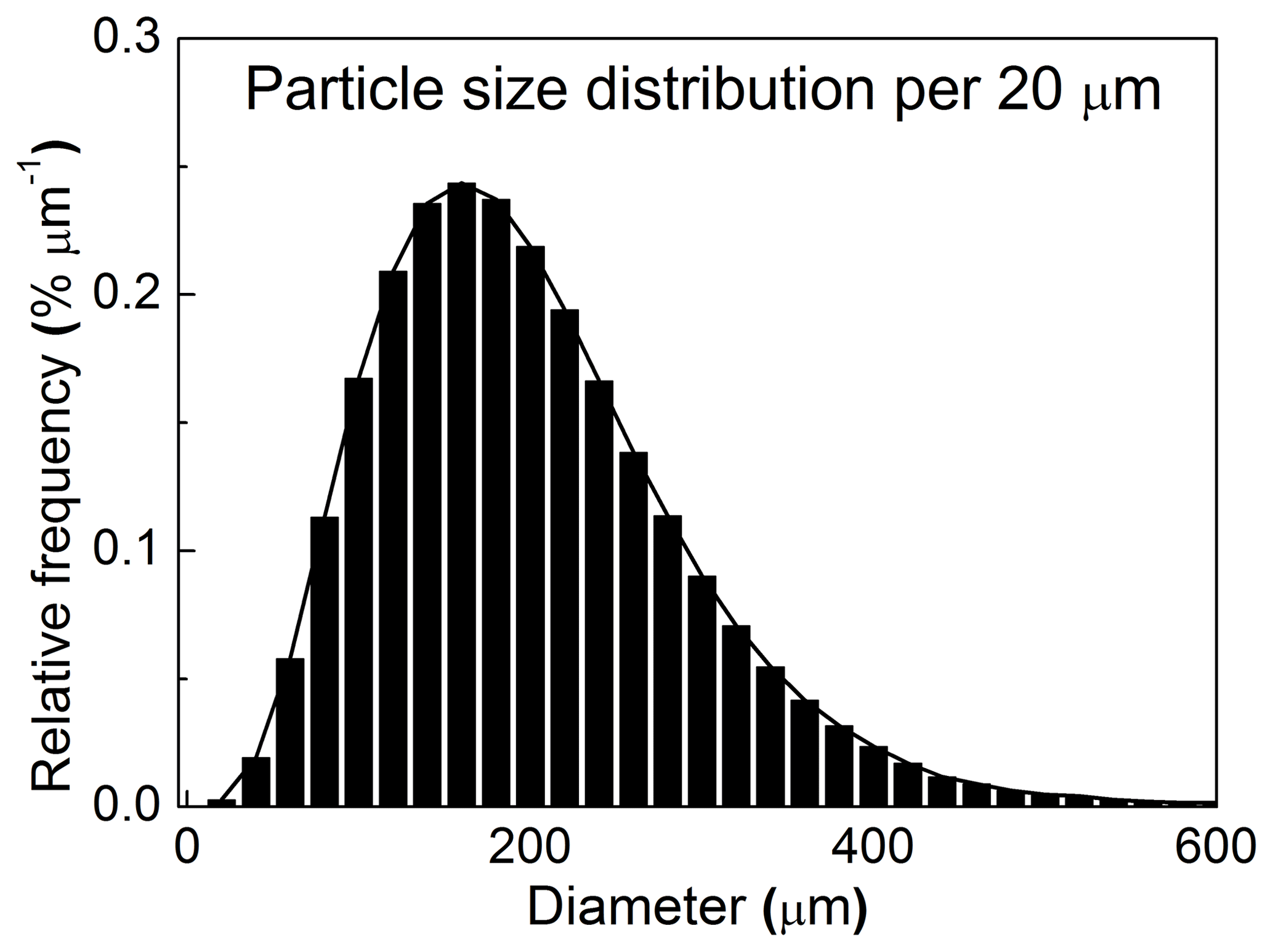
The size distribution of lift-off particles in drifting snow can be described well by the two-parameter gamma function (Budd, 1966; Gordon and Taylor, 2009; Nishimura and Nemoto, 2005; Schmidt, 1982)

$$\begin{array}{}\text{(17)}& {\displaystyle }{\displaystyle }f\left(d_{\mathrm{p}}\right)={\displaystyle \frac{d_{\mathrm{p}}^{{\mathit{\alpha }}_{\mathrm{p}}-\mathrm{1}}}{{\mathit{\beta }}_{\mathrm{p}}^{{\mathit{\alpha }}_{\mathrm{p}}}\mathrm{\Gamma }\left({\mathit{\alpha }}_{\mathrm{p}}\right)}}\exp \left(-{\displaystyle \frac{{\mathit{\beta }}_{\mathrm{p}}}{d_{\mathrm{p}}}}\right),\end{array}$$

where α_p and β_p are the shape and scale parameters of the distribution, respectively. In this simulation, the diameters of lift-off snow particles are given randomly from a gamma function with the parameters of α_p=4 and β_p=50, as shown in Fig. 1, which is also consistent with observed particle size distributions (Nishimura and Nemoto, 2005; Schmidt, 1982).

Figure 1 Size distribution of lift-off snow particles in this simulation.

3 Results and discussions

3.1 Model validation

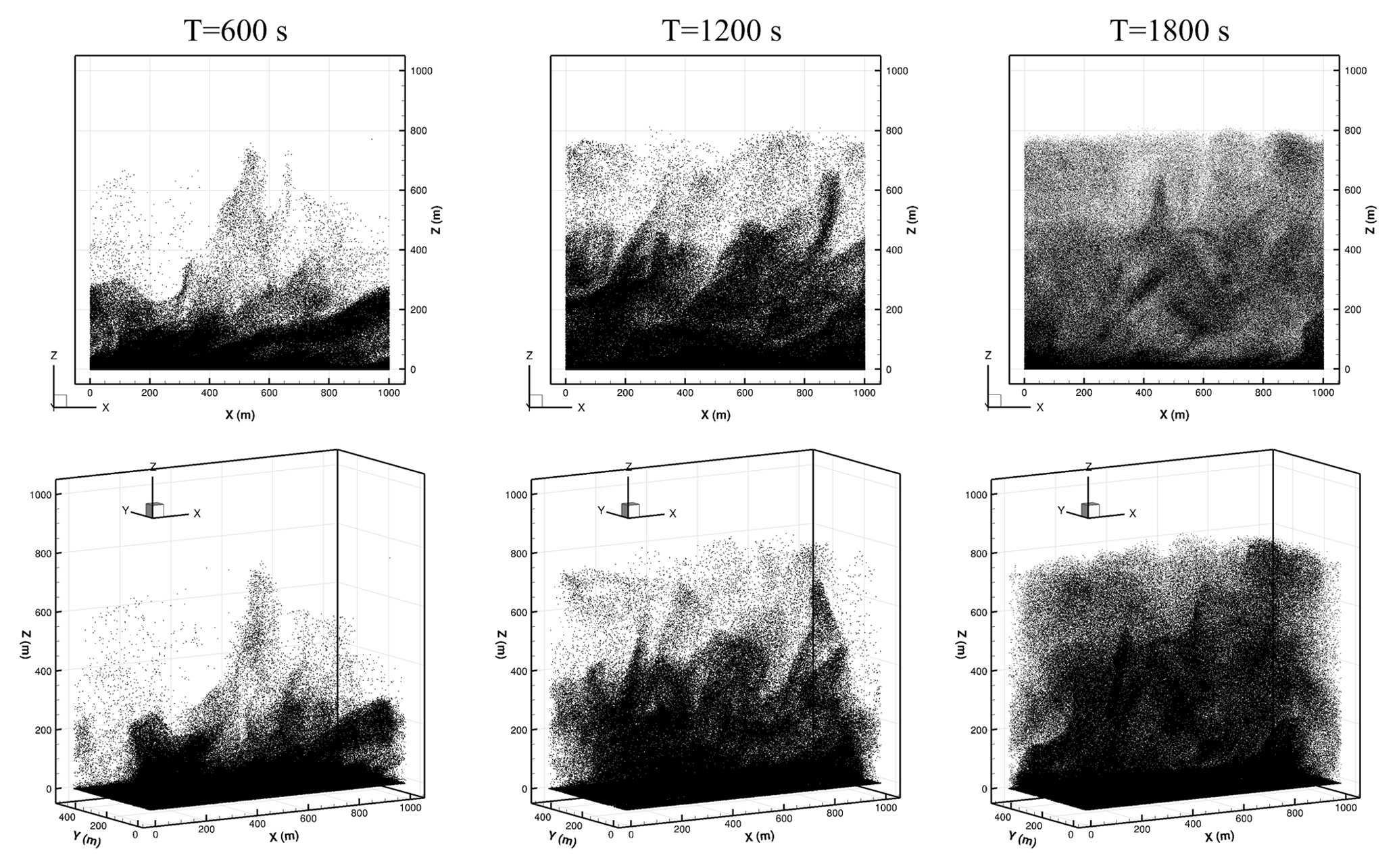
When drifting snow occurs in the atmospheric boundary layer, updrafts and turbulence fluctuations can send snow particles to high altitude, forming a fully developed drifting snowstorm. Figure 2 shows the drifting snowstorm in the atmospheric boundary layer at different moments, in which the friction velocity is $u_{*}=\mathrm{0.29}$ m s⁻¹ and dark spots represent snow particles. It can be seen that drifting snowstorms experience an evolution process from near the surface to high altitudes, in which particle concentration decreases with increasing height. The high concentrations of drifting snow cloud are generally below 500 m, though snow particles may reach up to approximately 800 m under this condition. This is also consistent with observations (Mahesh et al., 2003; Palm et al., 2011).

Figure 2 Drifting snowstorm at different moments under the friction velocity of 0.29 m s⁻¹.

Since a drifting snowstorm exhibits a different structure from bottom to top, the evolution of particle number density profile in the drifting snowstorm is shown in Fig. 3, which is also compared with measurements of Mann et al. (2000). From this figure, the thickness of the drifting snow layer obviously increases with time and almost approaches its steady state after 1200 s. At the same time, the particle number density basically decreases with height, which is consistent with the measurements of Mann et al. (2000) at various friction velocities. The predicted particle number density at the surface is much larger than at higher altitude and observations, mainly because the saltating particles are also included.

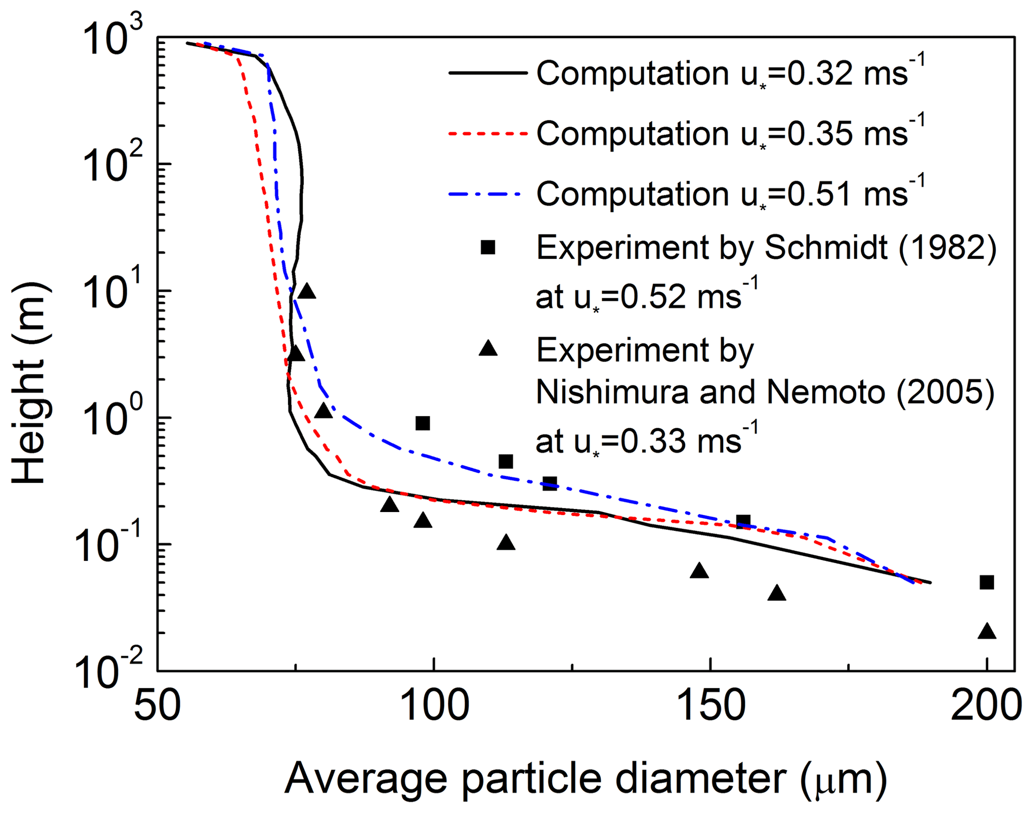
Generally, smaller particles are more likely to be transported higher in the air. Figure 4 shows the variation in modeled average particle diameter versus height, which is also compared with various field measurements (Nishimura and Nemoto, 2005; Schmidt, 1982). Similar to the field observations, the average particle size basically decreases with height at lower altitude but is almost constant above 1 m. The average particle diameter is approximately 75 µm, ranging from 1 m to hundreds of meters in height, which is also consistent with the measurements of Nishimura and Nemoto (2005).

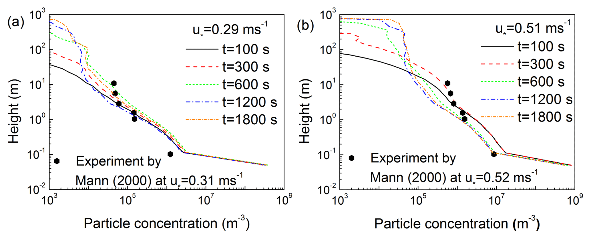
Figure 3 Evolution of particle number density under the friction velocities (a) 0.29 m s⁻¹ and (b) 0.51 m s⁻¹.

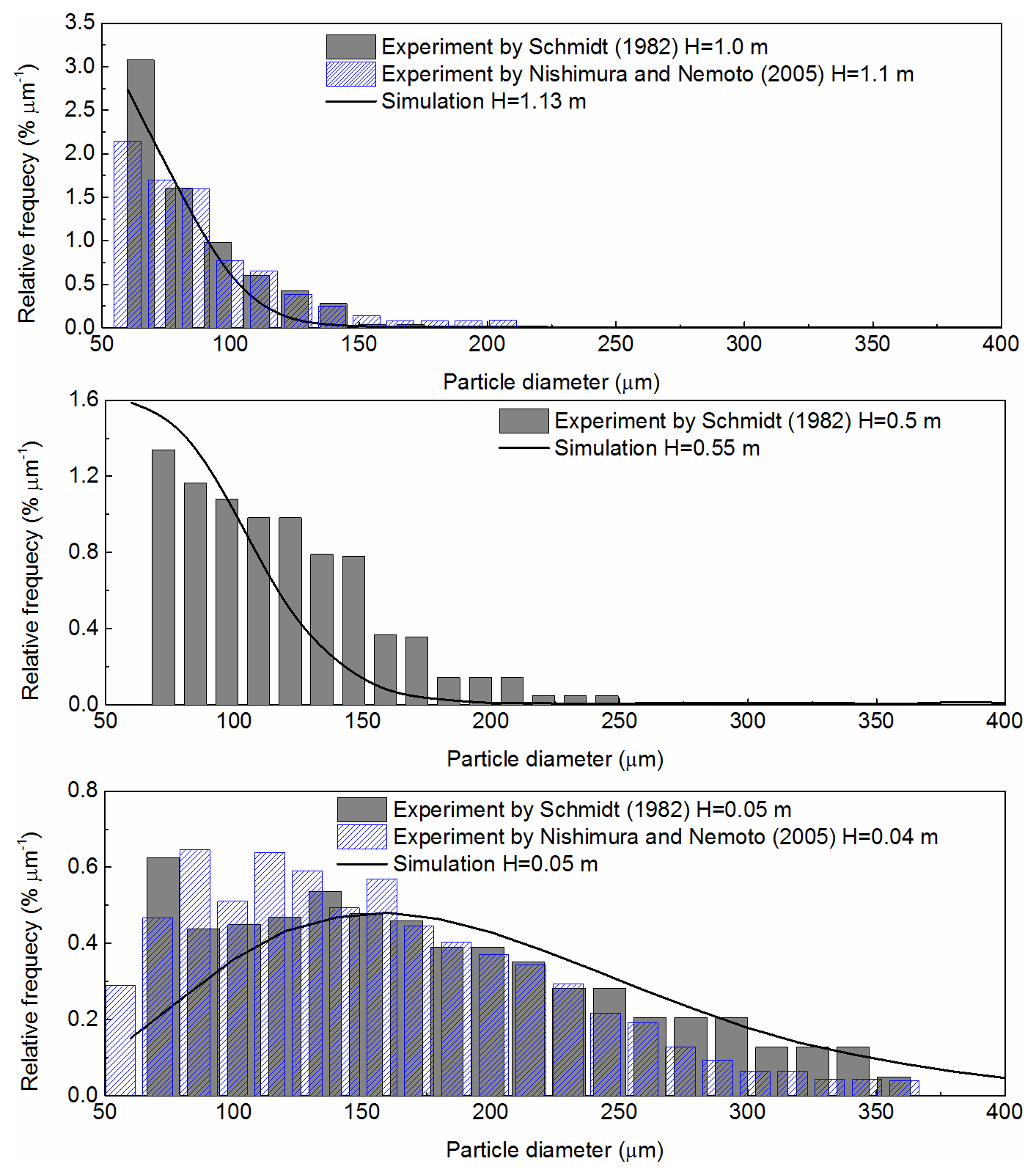
Then, the particle size distributions at various heights are also compared with experiment results. As shown in Fig. 5, the heights are 0.05, 0.5, and 1 m. The modeled particle size distributions at various heights are consistent with the measurements (Nishimura and Nemoto, 2005; Schmidt, 1982). Therefore, the established model is able to produce a large-scale drifting snowstorm.

In addition, it can be seen that the proportion of particles below 100 µm in diameter at 0.05 m is smaller than that of the experimental result. The reason could be that midair collisions, occurring frequently within the high-concentration saltating snow cloud at the near surface, play an important role in conveying larger particles to higher altitude (Carneiro et al., 2013). However, the midair collision mechanism is beyond the scope of the current study.

3.2 Snow transport flux

The snow transport flux is of great importance to predict the mass and energy balances of ice sheets. The total transport flux can be obtained from vertical integration of the snow transport flux profile.

Figure 4 Variation in average particle diameter versus height.

The profiles of snow transport rate, per unit area, per unit time, under various friction velocities are shown in Fig. 6a. It can be seen that the transport flux undergoes a sharp decrease with height at a lower altitude (e.g., below 1.0 m); however, the transport flux tends to decrease rather gently until almost the top of the drifting snowstorm, as shown in Fig. 6b, probably due to the large-scale turbulent motion and increasing wind speed with height. In other words, the suspension flux of drifting snow at higher altitudes, previously not observed, may be much larger than we previously thought. The mean horizontal wind speed profiles of the fully developed turbulent boundary layer under various friction velocities are shown in Fig. 7. The horizontal wind speed increases with height and changes into a constant above the boundary layer. The rapid decrease in the snow transport flux occurs at about the top of the turbulent boundary layer, mainly because turbulence becomes weaker above this height and fewer particles can be transported to a higher altitude.

In addition, the transition of snow transport flux profile at about 1 m should be mainly caused by the different motion states of particles with different particle sizes, as shown in Fig. 4. Above the critical height, particles generally follow the turbulent flow in the state of suspension because their gravities and relaxation times are small enough. However, plenty of larger particles at the near surface make the particles' velocity differ from the wind speed since particle inertia plays an important role.

In previous studies, only the transport fluxes at the near surface are commonly measured (Mann et al., 2000; Nishimura and Nemoto, 2005; Schmidt, 1982, 1984; Tabler, 1991); thus, the features of the entire transport flux profile are largely unclear, which may result in considerable uncertainties about the total transport flux. The proportions of suspension flux above a given height h_c (referred as Q_c) to the total suspension flux Q_s are shown in Fig. 7, in which snow particles below 0.1 m are not calculated (Mann et al., 2000).

From Fig. 8a, the contribution of Q_c to the total suspension flux is non-negligible under various h_c values, the proportion of Q_c when h_c=100 m to the total suspension flux has exceeded 30 % when the friction velocity is 0.46 m s⁻¹. At the same time, the proportion of Q_c to the total suspension flux increases with friction velocity but decreases with increasing h_c. From Fig. 8b, it can be seen that the proportion of Q_c to the total suspension flux is only slightly affected by the surface heat flux, which indicates that the structures of drifting snowstorm are not sensitive to the surface heat flux under this condition. The influence of surface heat flux is also weakened by the increasing friction velocity, mainly because larger friction velocity results in stronger turbulence under the actions of wind shear.

In this way, not only the snow transport flux, but also the sublimation of suspended snow particles should be reevaluated because the sublimation rate of snow particles higher in the air may be much larger than near the surface due to the lower air humidity and greater wind speed at higher altitude (Mann et al., 2000; Nishimura and Nemoto, 2005; Schmidt, 1982, 1984; Tabler, 1991).

3.3 Structures in a drifting snowstorm

In a drifting snowstorm, particles aggregate locally and produce special spatial structures (as shown in Fig. 2). These structures should be directly related to the turbulence structures present in the atmospheric boundary layer. Drifting snowstorms without atmospheric turbulence are shown in Fig. 9. This simulation is achieved by replacing the resolved wind speed at a particle's position $\left({\stackrel{\mathrm{̃}}{u}}_{\mathrm{i}}\left({\mathit{x}}_{\mathrm{p}}\right)\right)$ with a given value obtained from the standard logarithmic profile, and the other model settings and simulation procedures stay the same with other simulations. In this way, the effect of large-scale turbulent structures on the development of the drifting snowstorm vanishes. Compared with Fig. 2, drifting snow particles mainly travel at the near surface with a uniform spatial distribution when atmospheric turbulence is not included.

Figure 5 Particle size distribution at various heights.

It is known that snow particles will become suspended if the local vertical wind speed exceeds the terminal velocity of a particle. In a turbulent atmospheric boundary layer, there is a large number of turbulent structures with different scales and shapes. The vertical wind speed component of large-scale turbulence (namely, updraft) plays an important role in carrying snow particles to high altitude, while small-scale turbulence (e.g., the SGS fluctuating velocity) tends to spread particles from high concentration zones to low concentration zones. As shown in Fig. 10a, at the initial period of a drifting snowstorm, the structures in the drifting snowstorm are consistent with large-scale updrafts, and snow particles are mainly located in the updraft. With the further development of the drifting snowstorm, as shown in Fig. 10b, more snow particles are scattered around the updraft bubbles, although high-concentration particle clouds are still in the wind bubbles. When a drifting snowstorm approaches its saturated state, snow particle clouds are almost connected together with numerous high-concentration zones inside.

Figure 6 Variations in snow transport flux versus height.

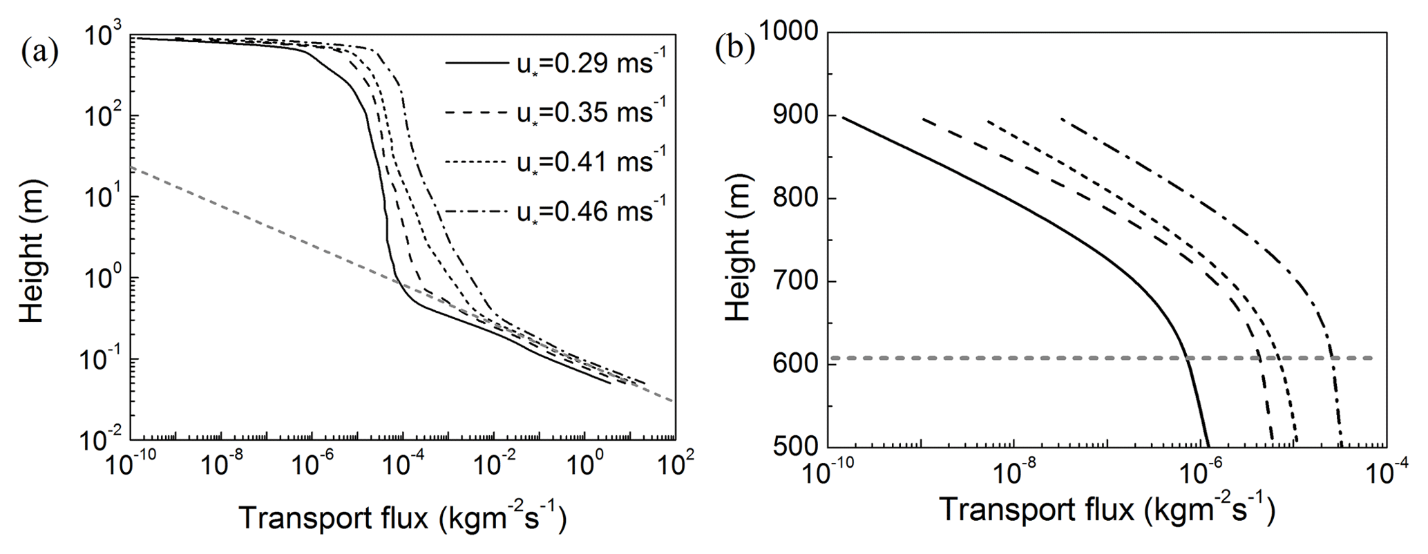
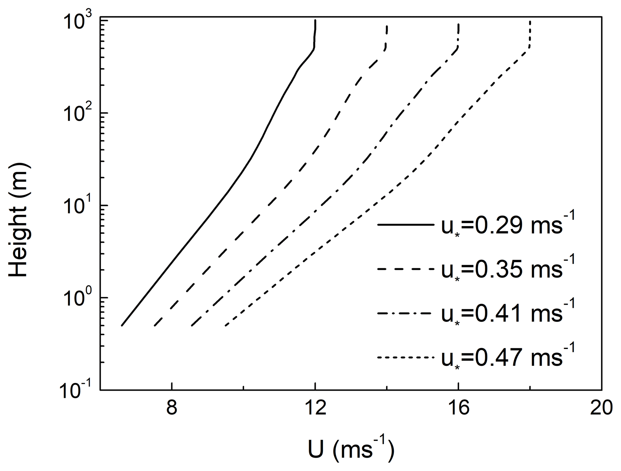
Figure 7 Horizontal wind speed profiles of the fully developed turbulent boundary layer under various friction velocities.

The evolution of the depth of a drifting snowstorm can be divided into three typical stages. In sequence, these phases are the rapid growth phase, the gentle growth stage, and an equilibrium state, as shown in Fig. 11. Here, the depth of a drifting snowstorm refers to the average height of the topmost particle during this period (100 s). The rapid growth stage is mainly driven by large-scale turbulent motion, while the turbulent diffusion by the SGS fluctuating velocity is the main contributor to the gentle growth stage. The duration of the second stage decreases with increasing friction velocity, which mainly comes from the stronger turbulent diffusion under larger friction velocities.

Figure 8 Proportion of suspension flux above h_c to the total suspension flux under (a) various friction velocities and (b) various surface heat fluxes Q_s.

Figure 9 Drifting snowstorm without atmospheric turbulence under a friction velocity of 0.35 m s⁻¹.

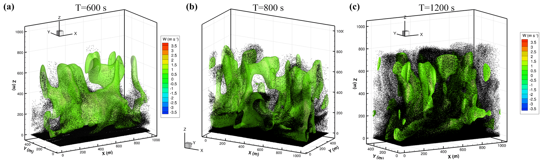
Figure 10 Evolution of the drifting snowstorm and vertical wind speed bubbles under a friction velocity of 0.35 m s⁻¹, and wind bubbles are the iso-surface of vertical wind speed with a value of 1.0 m s⁻¹ (corresponding to the critical wind speed at which the particle of mean particle size becomes a suspended particle since the maximum diameter of suspended particles is found to be approximately equal to the mean particle size of the lift-off particles).

At the same time, the time required for the drifting snowstorm to reach its maximum thickness decreases with friction velocity, ranging from about 1200 s to approximately 600 s when the friction velocity increases from 0.29 to 0.46 m s⁻¹. The thicknesses of saturated drifting snowstorms are almost constant with a value of approximately 900 m under different friction velocities, probably because the boundary layer depth as well as the surface heat flux are unchanged. Higher domain heights are also tested with the same model settings, and the thickness of the drifting snow seems basically unchanged. Drifting snowstorms with a difference in thickness may be achieved by changing the initial state of the air and surface heat flux. Thus, the final thickness of a drifting snowstorm should be largely dependent on the maximum height of atmospheric turbulence.

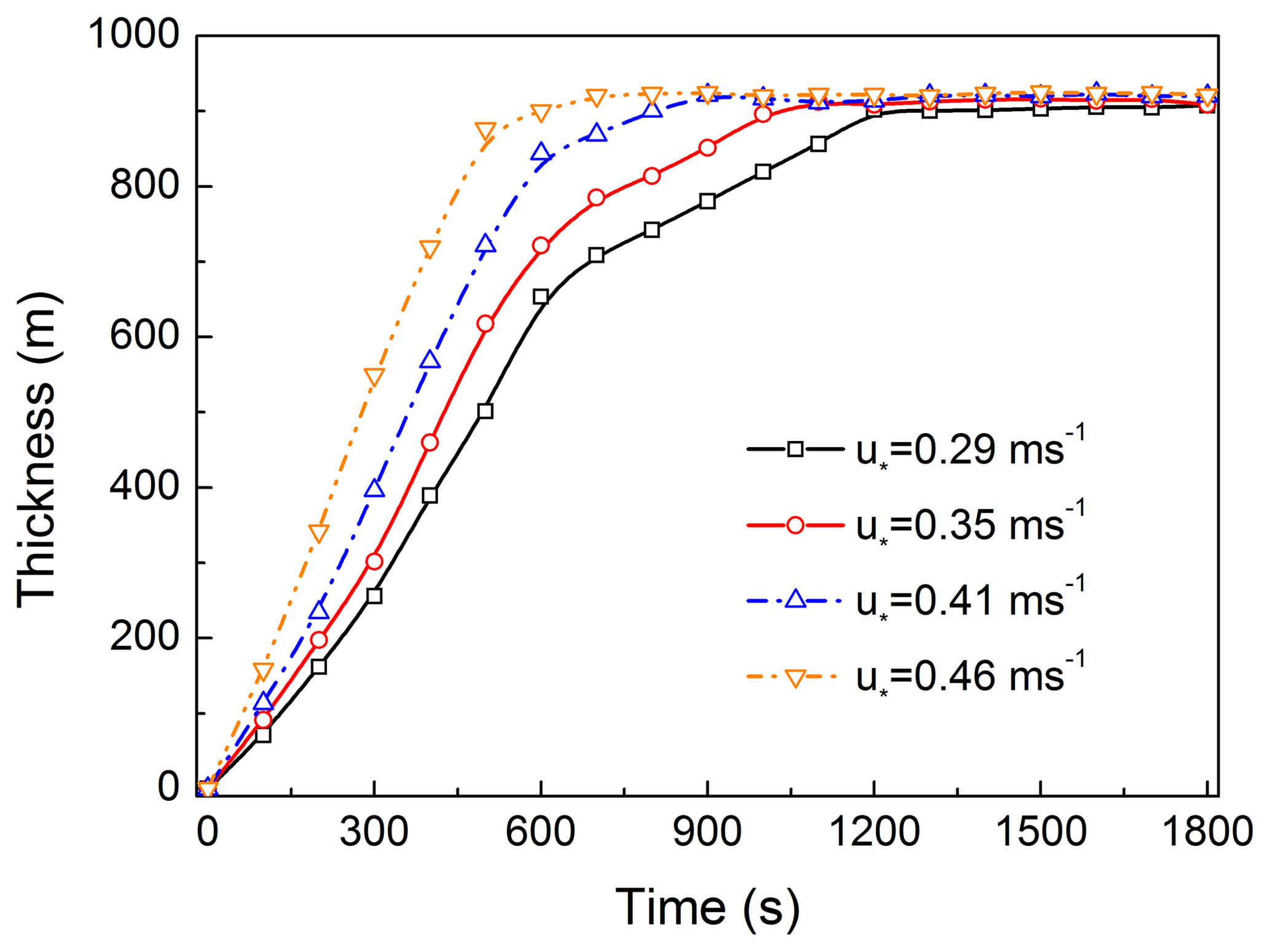
Figure 11 Time evolutions of the thickness of the drifting snowstorm under various friction velocities.

4 Conclusions

In this work, large-scale drifting snowstorms are simulated in a large-eddy simulation combined with a particle tracking model that includes subgrid-scale velocity fluctuations. A typical drifting snowstorm of several hundred meters in depth is generated, and the structure of the particle cloud with different concentrations is also produced. The transport flux profile has obviously different slopes near the surface compared to higher altitudes; that is, transport flux at the near surface decreases with height sharply, but decreases more gently at higher altitude. Previous studies may largely underestimate the total transport during drifting snowstorms.

At the same time, the evolution of the thickness of a drifting snowstorm generally contains three stages. Drifting snowstorm development generally begins with a rapid growth stage driven by large-scale atmospheric turbulent motions, followed by a gentle growth stage driven by the SGS fluctuating wind speed, before reaching an equilibrium stage when the drifting snow approaches a saturated state. The second stage becomes shorter with increasing friction velocity, mainly because stronger turbulence under higher friction velocity enhances the turbulent diffusion of particles.