the Creative Commons Attribution 4.0 License.
the Creative Commons Attribution 4.0 License.
 | 26 Nov 2018
Impact of assimilating a merged sea-ice thickness from CryoSat-2 and SMOS in the Arctic reanalysis
François Counillon
Laurent Bertino
Accurately forecasting the sea-ice thickness (SIT) in the Arctic is a major challenge. The new SIT product (referred to as CS2SMOS) merges measurements from the CryoSat-2 and SMOS satellites on a weekly basis during the winter. The impact of assimilating CS2SMOS data is tested for the TOPAZ4 system – the Arctic component of the Copernicus Marine Environment Monitoring Services (CMEMS). TOPAZ4 currently assimilates a large set of ocean and sea-ice observations with the Deterministic Ensemble Kalman Filter (DEnKF).
Two parallel reanalyses are conducted without (Official run) and with (Test run) assimilation of CS2SMOS data from 19 March 2014 to 31 March 2015. Since only mapping errors were provided in the CS2SMOS observation, an arbitrary term was added to compensate for the missing errors, but was found a posteriori too large. The SIT bias (too thin) is reduced from 16 to 5 cm and the standard errors decrease from 53 to 38 cm (by 28 %) when compared to the assimilated SIT. When compared to independent SIT observations, the error reduction is 24 % against the ice mass balance (IMB) buoy 2013F and by 12.5 % against SIT data from the IceBridge campaigns. The improvement of sea-ice volume persists through the summer months in the absence of CS2SMOS data. Comparisons to sea-ice drift from the satellites show that dynamical adjustments reduce the drift errors around the North Pole by about 8 %–9 % in December 2014 and February 2015. Finally, using the degrees of freedom for signal (DFS), we find that CS2SMOS makes the prime source of information in the central Arctic and in the Kara Sea. We therefore recommend the assimilation of C2SMOS for Arctic reanalyses in order to improve the ice thickness and the ice drift.
- Article
(11017 KB) - Full-text XML
- BibTeX
- EndNote


Sea ice plays an important role in the Arctic climate system because it prevents the rapid exchange of heat flux between the ocean and atmosphere. A decline and a thinning of the sea-ice cover has occurred in the past decades (e.g. Johannessen et al., 1999; Comiso et al., 2008; Stroeve et al., 2012) as well as an increase of deformation rates and drift speed (Rampal et al., 2009). It is expected that these changes will have significant impacts on the Arctic Ocean Circulation (e.g. Levermann et al., 2007; Budikova, 2009; Kinnard et al., 2011) and on the future human living environment (Schofield et al., 2011; Bathiany et al., 2016). The interpretation of such changes is severely hampered by the sparseness of observations, therefore the reanalyses that can provide continuous spatiotemporal reconstructions by assimilating existing observations into dynamical models have become increasingly popular tools. In addition, recent studies (Day et al., 2014; Guemas et al., 2014; Melia et al., 2015) have shown that sea-ice thickness (SIT) anomalies play an important role for the Arctic predictability up to seasonal time scale.
Satellite observations of sea-ice concentration (SIC) have been available since 1979 and have allowed an accurate monitoring of sea-ice extent (SIE) during that period. Data assimilation of SIC has constrained the position of the sea-ice edge (Lisæter et al., 2003; Stark et al., 2008; Posey et al., 2015), but large disagreements (e.g. Uotila et al., 2018) remain in the estimation of sea-ice volume because observations of SIT are very incomplete.
Until the 1990s, the only SIT measurements were sparse in situ measurements and submarine data. With new satellites, continuous estimates of SIT on basin scale have been achieved using satellite radar and laser altimeters: European Remote Sensing (ERS), Envisat and the NASA Ice, Cloud and land Elevation Satellite (ICESat). These were used to document the rapid thinning of sea-ice in the Arctic (Laxon et al., 2003; Kwok and Rothrock, 2009).
CryoSat-2, launched in April 2010, has been the first satellite dedicated to measure with high accuracy the sea-ice freeboard, from which SIT can be derived (Ricker et al., 2014; Tilling et al., 2016). However, the resulting SIT estimates are still very uncertain because of uncertainties in the snow depth (using climatology), snow penetration and sea-ice density (Kern et al., 2015; Khvorostovsky and Rampal, 2016). Those uncertainties are large for thin ice (<1 m). In parallel, satellite measurements from a passive microwave radiometer have retrieved SIT of thin ice (Martin et al., 2004; Heygster et al., 2009) from the Soil Moisture and Ocean Salinity (SMOS) satellite brightness temperature in the L-Band microwave frequency (1.4 GHz) (Kaleschke et al., 2010; Tian-Kunze et al., 2014). Although the consistency between the SMOS and CryoSat-2 estimates is still poor (X. Wang et al., 2016), a recent initiative has combined the two data sets in the Arctic (e.g. Kaleschke et al., 2015; Ricker et al., 2017) into a merged weekly SIT from the CryoSat-2 altimeter and SMOS radiometer (referred to as CS2SMOS, available online at http://www.meereisportal.de, last access: April 2017). The usefulness of assimilating this data set for reanalysis and operational forecasting needs to be tested.
In this study, the CS2SMOS will be assimilated into the TOPAZ4 forecast system, which is a coupled ocean–sea-ice data assimilation system using the Deterministic Ensemble Kalman Filter (DEnKF; Sakov and Oke, 2008). The Ensemble Kalman Filter has previously been demonstrated for assimilation of SIT data (Lisæter et al., 2007) of freeboard data (Mathiot et al., 2012) and of the CS2SMOS data (Mu et al., 2018) as well. TOPAZ4 is the Arctic Marine Forecasting system in the Copernicus Marine Environment Monitoring Services (CMEMS, http://marine.copernicus.eu, last access: 22 November 2018). Every day, it publishes a 10-day forecast of the ocean physics and biogeochemistry in the Arctic through the CMEMS portal. It also provides a long reanalysis from 1990 to the present – currently 2016 – that is extended every year. This reanalysis has been widely used and validated (Ferreira et al., 2015; Johannessen et al., 2014; Xie et al., 2017). Although SIT products are so far not assimilated into the TOPAZ4 reanalysis, the Arctic SIT distribution in TOPAZ4 shows some degree of spatial coherency with that of ICESat in spring and autumn of 2003–2008: it underestimates SIT (up to 1 m) north of the Canadian Arctic Archipelago and Greenland and overestimates it by approximately 0.2 m in the Beaufort Sea (Xie et al., 2017). Even though the SIT from ICESat has been reported too thick by about 0.5 m (Lindsay and Schweiger, 2015), the SIT from TOPAZ4 undoubtedly has spatial biases. Similar biases for SIT have been reported for other Arctic coupled ocean-ice models (Stark et al., 2008; Johnson et al., 2012; Schweiger et al., 2012; Yang et al., 2014; Smith et al., 2015, Q. Wang et al., 2016) and even reanalyses (Uotila et al., 2018). Xie et al. (2016) have tested assimilation of thin SIT (<0.4 m) from SMOS, and show that the assimilation slightly reduced the SIT overestimation near the sea-ice edge. The recent availability of the weekly SIT from CS2SMOS provides an opportunity for the TOPAZ4 to constrain better the SIT error in the Arctic. This study aims to identify a suitable practical implementation for assimilating C2SMOS data set and assess its usefulness for the Arctic reanalysis. Although it is expected that a better initialisation of SIT anomalies will enhance the predictability of the system, this is beyond the scope of this paper. A similar assessment over the same time frame has been carried out in the Arctic Cap Nowcast/Forecast System (ACNFS) by Allard et al. (2018) revealing significant improvements of bias and root mean square difference (RMSD) but little changes in ice velocity except in marginal seas. The proposed study in complementary to Allard et al. (2018) because the TOPAZ4 prediction system uses a more rudimentary sea-ice thermodynamics (no explicit ice thickness distribution) but a more advanced ensemble-based data assimilation method (TOPAZ4 uses strongly coupled data assimilation of ocean and sea ice, meaning that sea-ice observation will impact also the ocean and vice versa with a flow dependent assimilation method; see Penny et al., 2017; Kimmritz et al., 2018).
Section 2 describes the TOPAZ4 system: namely the coupled ocean and sea-ice model, the implementation of the EnKF and the observations used for data assimilation and validation. In Sect. 3, we carry out an observing system experiment (OSE) comparing the two reanalyses: one using the standard observation types used in operational setting and another assimilating the CS2SMOS in addition. Then the performance of the two runs is presented against both assimilated and non-assimilated measurements. Section 4 presents the impacts of assimilating the CS2SMOS on sea-ice drift and the integrated quantities for sea ice, and measures its relative impact compared to other assimilated observations. A summary is provided in the last section.
2.1 The coupled ocean and sea-ice model
TOPAZ4 is a forecasting ocean and sea-ice system developed for the Arctic, having been operational since the early 2000s (Bertino and Lisæter, 2008). It uses the Hybrid Coordinate Ocean model (HYCOM: version 2.2) developed at University of Miami, which has been successfully applied in global and regional oceans (Chassignet et al., 2003; Counillon and Bertino, 2009; Metzger et al., 2014; Xie et al., 2018). The model grid is constructed using conformal mapping (Bentsen et al., 1999) with a 12–16 km resolution shown in Fig. 1a. The model uses 28 hybrid layers with reference potential densities selected specifically for the North Atlantic and the Arctic regions (Sakov et al., 2012). The model is forced by atmospheric forcing from ERA-Interim. A barotropic inflow of Pacific water is imposed through the Bering Strait, which is balanced by an outgoing flow through the southern model boundary. It has an averaged transport of 0.8 Sv, and varies seasonally with a minimum (0.4 Sv) in January and a maximum (1.3 Sv) in June consistently with observations (Woodgate et al., 2005). The model accounts for river discharge, for which a seasonal climatology is estimated by feeding the run off from ERA-interim (Dee et al., 2011) into the Total Runoff Integrating Pathways model (TRIP, Oki and Sud, 1998) over the period 1989–2009.

Figure 1(a) Horizontal resolution (km) of the model grid in the Arctic (>60∘ N). The small yellow squares are the locations of IceBridge campaigns during the experimental period. The marginal seas are as follows: Beaufort Sea (BS; also shown with the blue line), Chukchi Sea (CS), East Siberian Sea (ESS), Laptev Sea (LS) and Kara Sea (KS); and the other regions are as follows: Canadian Arctic Archipelago (CAA), Svalbard Island (SI) and Fram Strait (FM). The four purple markers (star, circle, triangle and diamond) are the deployment location of IMB buoys (2013F, 2014B, 2014C, and 2014F respectively) with the following trajectory shown as black solid curves. The three red squares are the fixed locations of the BGEP moorings (14A, 14B and 14D, respectively). (b) Trajectories of International Arctic Buoy Program buoys drift during the experimental period. The solid red line delimits the coastal areas excluded in the analysis.
A simple sea-ice model using a one-thickness category has been coupled to HYCOM. The sea ice and the ocean are thus coupled every 3 h and exchange momentum, salt and heat on the ocean model's Arakawa C-grid. The sea-ice thermodynamics treat precipitations on ice as snow whenever surface air temperature is below zero (Drange and Simonsen, 1996). The ice dynamics uses the elastic–viscous–plastic rheology (Hunke and Dukowicz, 1997) with the modification suggested by Bouillon et al. (2013). There is a 0.1 m limit in the model for the minimum thickness of both new ice and melting ice.
2.2 Implementation of the EnKF in the TOPAZ4 system
The TOPAZ4 system uses a deterministic Ensemble Kalman Filter (DEnKF, Sakov and Oke, 2008), which solves the analysis without the need to perturb the observations and is therefore a square-root filter implementation of the EnKF. In the DEnKF, if the model state is represented by x, the ensemble mean is updated by the following equation:
where the superscripts “f” and “a” refer to the forecast and the analysis, respectively. Following Xie et al. (2017), the model state vector x contains 3-dimensional ocean variables in the native hybrid coordinates (u and v components of the current velocities, temperature, salinity and model layer thickness), the 2-dimensional ocean variables (u and v components of the barotropic velocities, barotropic pressure and mixed layer depth) and three sea-ice variables: ice concentration, ice thickness and snow depth. The assimilated observations are represented by the vector y without perturbation, and the observation operator H projects the model variables on the observation space. The misfit between the model and the observation – the bracket term in Eq. (1), is the innovation. The Kalman gain K is calculated by
where Pf is the background error covariance matrix, R is the observation error covariance matrix and the superscript “T” denotes a matrix transpose. The background error covariance is approximated from the ensemble anomalies A (where , , N being the ensemble size) as . Here, X denotes the ensemble of model states. The observation errors are assumed to be uncorrelated (i.e. the matrix R is diagonal). While this practical assumption is not valid for interpolated observations, a diagonal approximation combined with an inflation of the observation error can make a reasonable approximation when the error spatial structure is unknown (Stonebridge et al., 2018). A localization is used in order to reduce the sampling error with a radius of 300 km and a polynomial tapering function (in a local analysis framework).
The practical implementation of the model and its perturbations follow Sakov et al. (2012): the model errors include joint perturbations of winds and heat fluxes as originally recommended by Lisæter et al. (2007). The precipitation perturbation has however been increased from 30 % to 100 %, following a log-normal probability distribution of errors (Finck et al., 2013), which also increased the spread of ice thickness.
2.3 Observations for assimilation and validation
The following observations are assimilated sequentially every week in the TOPAZ4 system (Xie et al., 2017): along-track sea level anomaly; in situ profiles of temperature and salinity; gridded Operational Sea Surface Temperature and Sea Ice Analysis (OSTIA) SST; Ocean and Sea Ice Satellite Application Facility (OSI-SAF) sea-ice concentration and sea-ice drift from satellite observation (Lavergne et al., 2010). All measurements are retrieved from CMEMS, http://marine.copernicus.eu (last access: April 2017), and are quality controlled and high-resolution observations are “superobed”: all observations falling within the same grid cell are averaged and the observation uncertainty is reduced accordingly (Sakov et al., 2012). For SST and ice concentration, we only retain the observation on the last day of the assimilation cycle. Similarly, only the sea-ice drifts during the last 2 days of the assimilation cycle are assimilated.
The weekly SITs of CS2SMOS were retrieved from http://data.meereisportal.de/maps/cs2smos/version3.0/n (last access: April 2017) on the period from March 2014 to March 2015. This product is gridded with a resolution of approximately 25 km. The provider uses optimal interpolation to blend the measurements of CryoSat-2 and SMOS based on their uncertainties and their spatial covariance. An estimate of the observation error is provided with the data set but only accounts for the errors related to the merging and interpolation (Ricker et al., 2017). As such, we expect that this observation error is underestimated since it misses both the sensor errors and the model-related representation errors. In particular the mapping is based on a no-bias assumption and error estimates do not account for inconsistencies between the two satellites, like those reported by X. Wang et al. (2016) and Ricker et al. (2017). With an EnKF assimilation system, underestimating the observation error leads to an underestimation of the ensemble spread and makes the system suboptimal, leading in the worst case to system divergence. Underestimating the errors of one data type also lessens the impact of the other assimilated observations since they compete for the control of a finite number of degrees of freedom. This issue will be addressed in Sect. 4.3. On the other hand, Oke and Sakov (2008) showed that the performance of the EnKF does not degrade much when observation error is overestimated. It is therefore necessary to increase the observation error to a level at least as high as the optimal value for the performance of the filter (Desroziers et al., 2005; Karspeck, 2016).
In order to estimate the representation error for the SIT observation, we have performed a preliminary sensitivity assimilation experiment for November 2014. We used the diagnostics by Desroziers et al. (2005) as an indicative lower limit for the observation error in the TOPAZ4 system based on the misfits to the CS2SMOS data. Desroziers et al. (2005) estimate the optimal observation error as the following matrix:
where p is number of data assimilation steps in the sensitivity run (here 4), and yj represents the observed SIT from CS2SMOS at the jth assimilation time. Here, the terms and represent the ensemble mean of the analysis and forecast states. In Fig. 2, the diagnosed observation errors from Desroziers et al. (2005) are larger than the mapping error included in CS2SMOS, but still do not account for biases in the CryoSAT2 and SMOS observations. The CS2SMOS mapping error is particularly low for sea ice below 0.5 m: about 4 times lower than the uncertainties obtained by error propagation in the SMOS processing chain (used in Xie et al., 2016), which would make the assimilation of SMOS SIT too strong. The Desroziers diagnosed errors gradually increase with ice thickness, although they vary unrealistically for SITs above 3 m, possibly due to low counts of either modelled or observed ice thickness in certain thickness ranges. In view of the above considerations, we have added a cautious correction term to the CS2SMOS mapping error estimate, which simply increases linearly with the observed SIT.
where dSIT is the observed sea-ice thickness. At low SIT, the resulting values are slightly higher than those used in Xie et al. (2016) and comparable to the Desroziers diagnostics. At SITs of 1.5 m, for which SMOS and CS2SMOS overlap, the added correction is comparable to reported differences between the two satellites: about 20 cm in the Beaufort Sea and 1 m in the Barents Sea; see Table 3 in Ricker et al. (2017). Tilling et al. (2018) show that the standard deviations between the CryoSat-2 and independent measurements are between 30 and 70 cm depending of the source of observation and increase with ice thickness (their Fig. 16). It should be noted however that the processing of CryoSat2 data differs in CPOM and AWI's algorithms. The total observation error including the added term is shown with blue-squared line in Fig. 2. In the following, we will only use the corrected observation error for the CS2SMOS SIT.
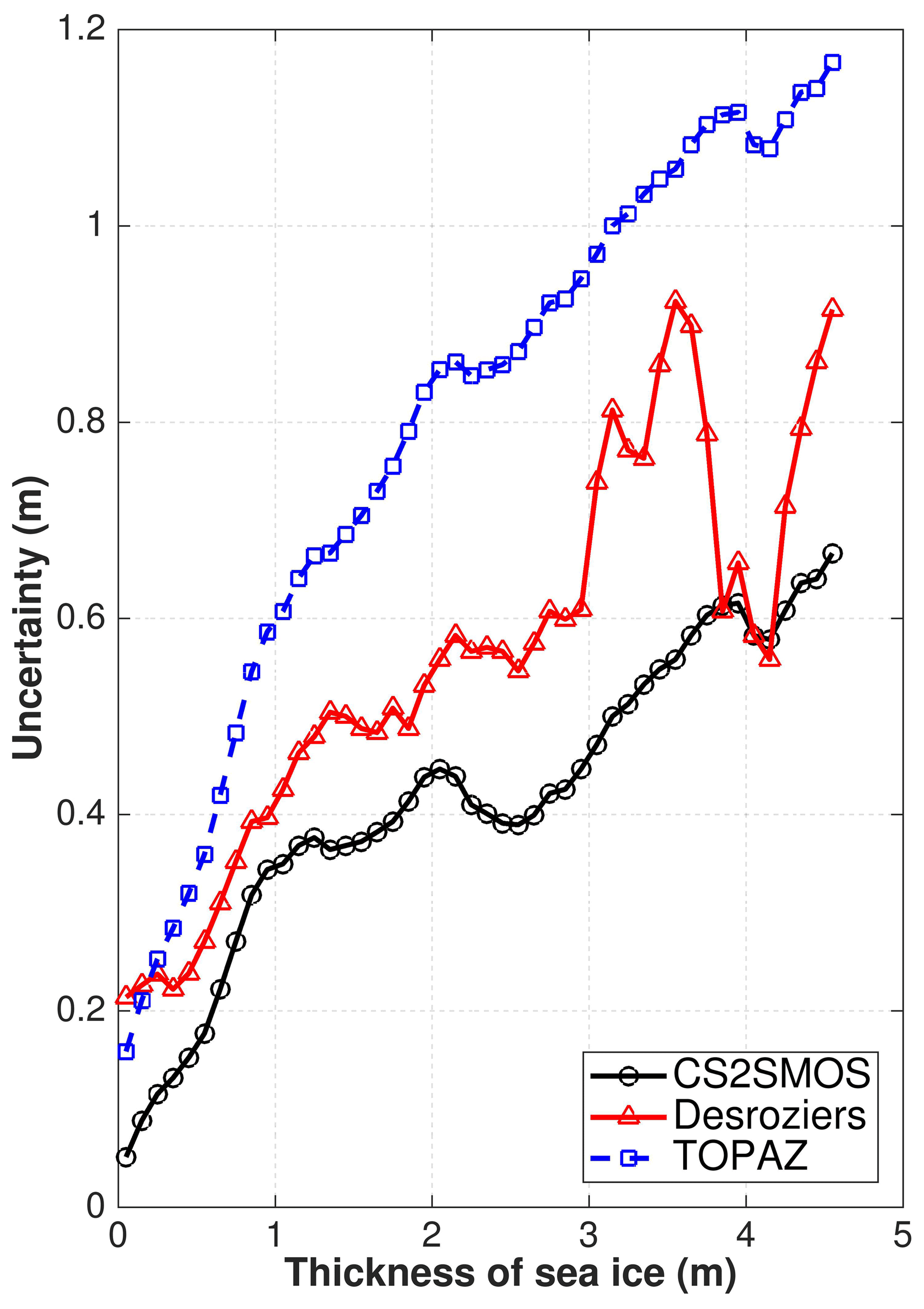
Figure 2Observation error uncertainties as a function of sea-ice thickness for the original CS2SMOS data set (black line), the estimated observation error using the Desroziers diagnostics with red-triangle line (see Eq. 3) and the one used in the TOPAZ Test run with blue-square, with an additional error term as Eq. (4) to the original uncertainty.
3.1 Experiment and independent observations for validation
A parallel OSE is conducted from 19 March 2014 until end of March 2015. The two assimilation runs cover two special time periods: the onset of ice melting in March–April 2014 following by a data period free of CS2SMOS, then a whole cold season from October 2014 to March 2015. The control run named the Official run uses the standard observational network in the TOPAZ4 system (Xie et al., 2017), which assimilates on a weekly cycle the SLA, SST, in situ profiles of temperature and salinity, SIC and sea-ice drift (SID) data. Another assimilation run named the Test run includes as well the SIT from CS2SMOS.
We discard the SIT closer than 30 km from the coast to account for differences of coastlines between the model and observations. The innovation of SIT in Eq. (1) is calculated in terms of sea-ice volume:
where dSIT is the observed SIT from CS2SMOS as in Eq. (4), and is the ensemble mean of ice volumes forecasted by model. The f and h are SIC and ice thickness within the grid cell, respectively. We assume the observation error is uncorrelated (R in Eq. 2 is diagonal). Although the minimal thickness in the model is set to 0.1 m, the ensemble mean from 100 model members can be as thin as 1 mm, so that we only reject the observed SIT if it is equal to 0. Every week, the SITs from CS2SMOS are considered to be at the analysis time, neglecting the time delay. The associated errors due to the sea-ice motions or thermodynamic growth or melt of sea ice within 1 week remain small compared to the large SIT biases targeted in the present exercise.
In the following, we investigate the misfits of the forecasted model states by evaluating the bias and the RMSD:
where L is the total number of assimilation cycles during the study, is the ensemble mean model state at the ith time, which is compared to the observations yi.
Three types of independent SIT observations are used for validation. First, the drifting ice mass balance buoys (IMB: http://imb-crrel-dartmouth.org/imb.crrel/buoysum.htm, last access: April 2017, Perovich and Richter-Menge, 2006). Four IMB buoys are available during the experimental time period (2013F, 2014B, 2014C and 2014F) and their trajectories are shown in Fig. 1a. Second, three upward looking sonar (ULS) buoys funded by the Beaufort Gyre Exploration Project (BGEP; see http://www.whoi.edu/beaufortgyre, last access: July 2018) have been moored in the Beaufort Sea. Their locations are shown with the red squares in Fig. 1a. They estimate the sea-ice drafts since October 2014. Third, the NASA IceBridge Sea Ice Thickness Quick Look data (https://nsidc.org/data/icebridge, last access: 22 November 2018) collected in aerial campaigns estimate the SIT in spring (Kurtz et al., 2013) with a better spatial coverage. The locations of the quality-controlled SIT observations from IceBridge for March and April of 2014 and 2015, are shown with the yellow squares in Fig. 1a.
3.2 Validation against CS2SMOS and innovation diagnostics
The first assimilation time is the 19 March 2014 and the last is the 25 March 2015. The monthly SITs from the two OSE runs are compared to CS2SMOS in Fig. 3. The SITs in April 2014 are presented for comparison in the upper row of Fig. 3. In the Official run, the thick sea ice to the north of the CAA is underestimated but thickens slightly in the Test run: the 3 m SIT isoline covers a wider area, in better agreement with the observations. The areas of thinner sea ice north of the Barents Sea, west of the Kara Sea, and the coast of the Beaufort Sea, which were too thick in the Official run, have all been improved also shown by reduced area delimited by the isolines of 1 or 2 m SIT in the Test run.

Figure 3Monthly SIT from CS2SMOS, column (a), Official run, column (b), and Test run, column (c) in April 2014, November 2014, and March 2015, respectively. The mean SIT estimated for the area north of 80∘ N is indicated between parentheses (unit: m). The dashed lines are isolines of 1, 2, 3 and 4 m SIT, respectively.
After summer of 2014, measurements of SIT from CS2SMOS restart at the end of October. Results are presented for November 2014 in Fig. 3: the thick sea ice in the Central Arctic has been further improved in the Test run. The thickest sea ice (>3 m) is located near the northern coast of Canada instead of north of Greenland in the Official run. The averaged SIT in the Test run around the North Pole (>80∘ N), is increased from 1.3 m in the Official run to 1.6 m, which is closer to CS2SMOS by 43 %. In the marginal zones – East Siberian Sea, Laptev Sea, and Kara Sea – the SITs in the Official run are too thin, but are thicker in the Test run. Improvements in marginal seas are due to the contribution of SMOS, while improvements in the ice pack are more likely due to CryoSat-2.
In the last month of the experimental period (March 2015), the thick sea-ice pattern in the Test run, shown as the 2 m isoline, is more similar to CS2SMOS. The maximal SIT within the 4 m isoline is located north of the CAA in the Test run and in CS2SMOS, while in the Official run it spreads further out from the northern coast of Canada to north of Greenland. In addition, the SIT north of the Fram Strait is thicker than in the Official run. The SIT is similarly improved near the coast of the Beaufort Sea and to the northwest of Svalbard. As expected with data assimilation, the Test run agrees clearly better with the assimilated product. Those improvements are largest in the ice pack and in the marginal seas, where the model deviates considerably from the CS2SMOS SITs. On the contrary, the thickness near the sea-ice edge is not strongly impacted by the assimilation.
The above results are confirmed quantitatively by comparing misfits of weekly SIT from the two runs with the corresponding CS2SMOS observations. Time series of bias and RMSD calculated as in Eqs. (6) and (7) are shown in Fig. 4a. In the beginning of the period, the SIT RMSD in the Test run decreases quickly from 0.6 to 0.4 m before the observations are interrupted for the summer. The biases are reduced equally in both runs. After the observations resume in the end of October 2014, the SIT RMSD is comparable between the two runs but the bias is slightly lower in the Test run. There is large spike in the bias and RMSD for both systems that relates to an inaccuracy of the CS2SMOS observations (see Sect. 4.2). After the spike, the RMSD and bias in the Test run are lower than in the Official run. The bias in the Test run converges to 0 and fluctuates around that level but this is probably not due to the assimilation since the bias in the Official run also converges to 0 during that time. This is rather due to the compensation of seasonal and regional errors. On average, the SIT bias (too thin) is decreased from 15 to 5 cm by the assimilation of CS2SMOS. The RMSD of SIT is 38 cm in the Test run, which corresponds to a reduction of 28.3 % relative to the error in the Official run.

Figure 4(a) Bias (dotted line) and RMSD (solid line) of SIT in the two runs – Official (blue) and Test (red) – based on weekly averaged reanalysis and CS2SMOS observations. The time-averaged bias and RMSD are indicated (Official/Test). (b) SIT innovation statistics in the Test run in the Arctic region (>60∘ N) from 19 March 2014 to end of March 2015. The blue-squared (red reverted-triangle) line represents the mean (RMSD) of the innovation. The green squared line represents the ensemble spread and the purple reverted-triangle line is the diagnosed total uncertainty (see Eq. 8). The gray-crossed (gray-circled) line is the number (RMSD observation error) of assimilated observations.
The innovation statistics taken at each assimilation time are used to evaluate how well our data assimilation system is calibrated. In the reliability budget of Rodwell et al. (2016), the total uncertainty of an ensemble data assimilation system is calculated as follows:
where the bias term – i.e. the mean innovation (shown as blue-circled lines) – is calculated as in Eq. (6) at a given assimilation time step, while σen and σo represent respectively the ensemble spread and the standard deviation of the observation errors at the same assimilation time. If the data assimilation system is reliable, the diagnosed total uncertainty should be close to the RMSD, formulated in Eq. (7). Figure 4b shows that the pink and red lines are evolving reasonably in phase but that the diagnosed error σdiag is twice larger than the RMSD, meaning that our system is overdispersive. The error budget shows that the observation error (σo) itself is too large, suggesting that the offset term in Eq. (4) is overestimated, which we do not expect as a serious problem as explained above.
The innovation statistics for SIC are mostly identical in the two runs (not shown), the mean misfits for SIC vary around ±4 % and are most of the time lower than 12 %, which is consistent with the evaluation of the TOPAZ4 reanalysis in Xie et al. (2017). It is somewhat disappointing that improvements of ice thickness do not yield visible benefit to ice concentration, but on the other hand a degradation could also have been possible in case the thermodynamical model had been over-tuned to an incorrectly simulated thickness. It should also be noted that the innovations statistics of SST and SLA are also indiscernible in the two runs and not shown either.
3.3 Validation against independent SIT observations
3.3.1 Ice mass balance buoys
Four IMB buoys are available as independent validation of the impact of the assimilation of CS2SMOS. The buoys are drifting in the Canadian Basin (Fig. 1a), and only one buoy (2013F) lasted during the whole experimental time period shown (Fig. 5a). This buoy exhibits the seasonal variability of SIT: it reaches 1.5 m in spring 2014, decreases down to 1.0 m in September and rises again to 2 m in March 2015. The seasonal SIT cycle of the Official run shows excessive seasonal variability, with a thin bias in summer 2014 and a thick bias during the two winters. In the Test run (shown as the red-dashed line) the seasonal cycle is dampened and more consistent with the observations. The bias is still quite large around March–April and remains so even at the end of the study period. It should be noted that the impact of CS2SMOS seems largest in summer, when no observations are assimilated. This illustrates the persistent effects of winter SIT improving the predictability of the summer Arctic sea ice as shown in Mathiot et al. (2012). When CS2SMOS is assimilated again in the fall 2014, the Test run initially slightly overestimates the SIT measured at the buoy compared to the Official run but is slowly improving as the data is assimilated. The time-averaged SIT RMSD for buoy 2013F is reduced from 0.33 m in the Official run down to 0.25 m in the Test run, a reduction by 24.2 %.
Two other buoys (2014B and 2014C) cover the early months of the experimental period. The two runs are initially biased with a too thick SIT by 0.5 and 0.2 m compared to 2014B and 2014C. At buoy 2014B, there is a slight error reduction during the assimilation period that continues beyond the assimilation window, similarly to buoy 2013F. At buoy 2014C however, although the error is reduced during the analysis period, the two assimilation runs converge during the summer. At these three buoys the assimilation corrects the mean SIT values and the amplitude of the seasonal cycle but has little influence on the phase of the seasonal cycle.
The buoy 2014F covers the last 6 months of the experimental period. At that buoy, the assimilation seems increase the errors. It should be noted however that the constant SIT at buoy 2014F seems unlikely or not representative of the area.
3.3.2 The BGEP mooring buoys
In order to convert the sea-ice draft measured by ULS from the BGEP buoys to SIT, we used the balance equation as in Tilling et al. (2018):
where dSIT is the sea-ice thickness, di is sea-ice draft, hs is snow depth, ρi is sea-ice density, ρs is snow density and ρw is seawater density. The above densities are set to 900, 300 and 1000 kg m−3 as in the TOPAZ model. di is the sea-ice draft measured by ULS at the fixed locations (see Fig. 1a). The snow depth is taken from the model daily snow depths, averaging the two model runs and interpolating at the buoys' locations.
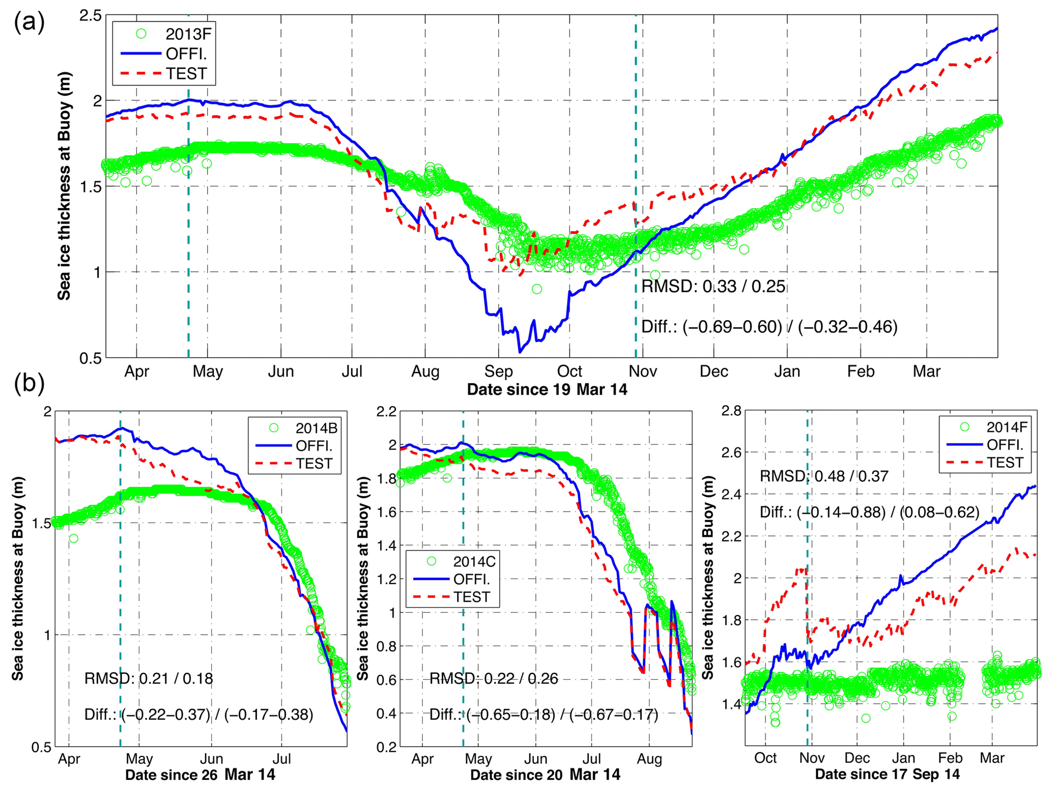
Figure 5Time series of SIT along the trajectories of IMB buoys (a: 2013F; b: 2014B, 2014C and 2014F). Measured SIT (green), daily averages from the Official run (blue line) and the Test run (red line). The vertical cyan-dashed lines indicate the winter period when C2SMOS is assimilated in the Test run.
The SIT time series of the measurement and of the two runs are shown in Fig. 6, from October 2014 onwards. The gray error bars depict the daily standard deviation. The data indicates an increasing SIT from around 0.5 m in October 2014 to nearly 2 m in March 2015. The observed SIT at mooring 14D shows a very large daily variability from end of October to November 2014, especially compared with that of moorings 14A and 14B.
The weekly SITs from CS2SMOS match well the data with RMSDs of 15, 19 and 39 cm during the 6 months, which is lower than in the two model runs. Still, the SIT from CS2SMOS overestimates SIT from October 2014 to mid-January 2015 compared to the mooring 14B, and between in October and November of 2014 for mooring 14A. The SITs in the Official run are overestimated in all three locations. The SIT RMSDs are 41, 23 and 51 cm, respectively, compared to SIT measurement from the three moorings. The SITs in the Test run are closer to observations, thanks to the data assimilation of the SIT from CS2SMOS. The SIT RMSDs in the Test run are 25, 33 and 36 cm for moorings 14A, B and D, respectively. The error is reduced for moorings 14A and 14D compared to the Official run but increases for mooring 14B, mostly due to the initial mismatch between CS2SMOS and the mooring. Similarly to the comparison with IMB buoys, moorings suggests that error of SIT in the Beaufort Sea is reduced by assimilation of CS2SMOS.
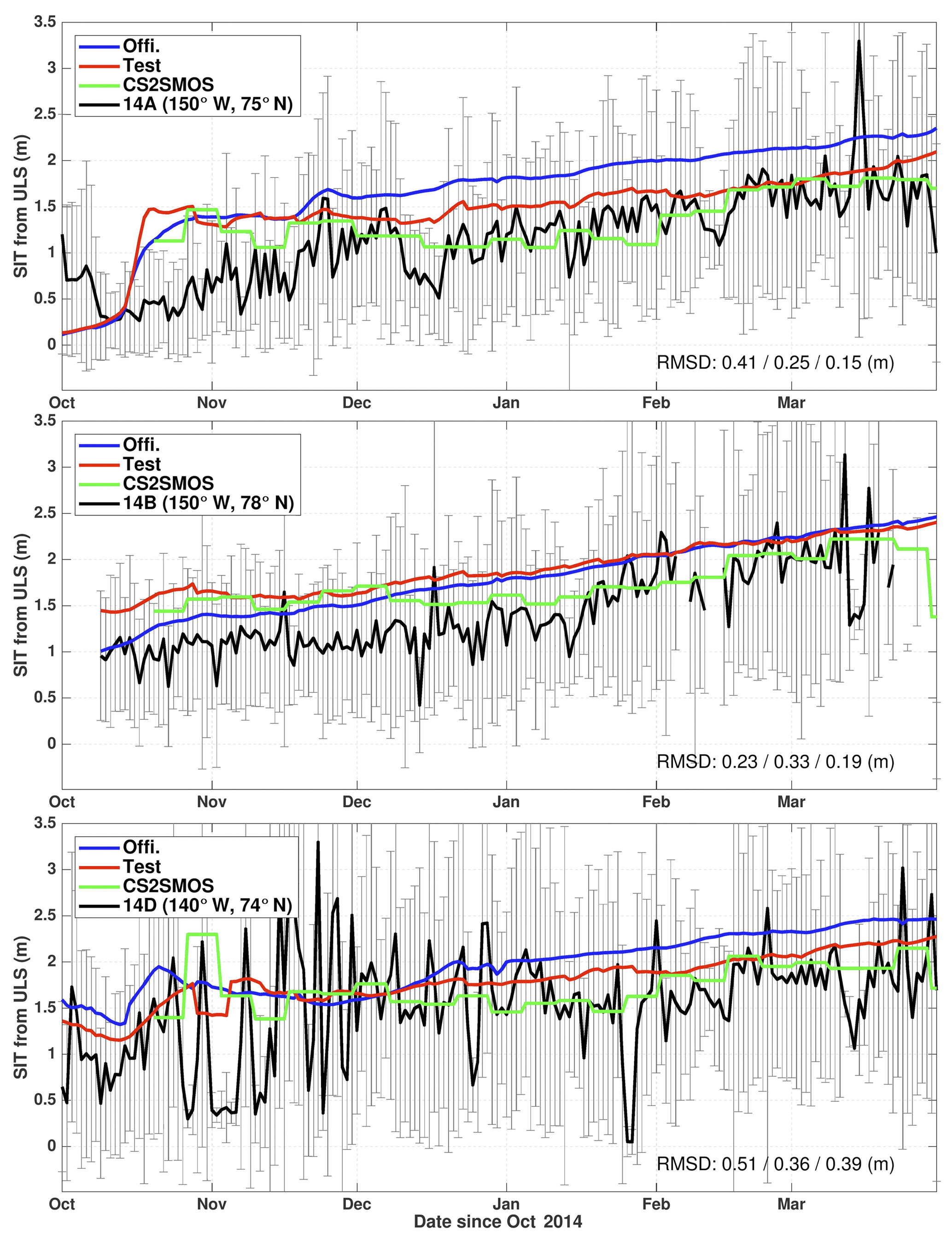
Figure 6Daily series of SIT (black line) at the BGEP mooring (14A, 14B, and 14D) compared with the two model runs – Official (blue line) and Test (red line) – and the weekly observed by CS2SMOS (green line). The black line represents the daily average at the mooring location with the standard deviation shown as the error bar. The RMSDs of the Official run, Test run and CS2SMOS are respectively indicated on the bottom of each panels.
3.3.3 IceBridge quick look
Another independent observation of SIT with better spatial coverage is the SIT Quick Look data from airborne instruments during NASA's Operation IceBridge campaign (Kurtz et al., 2013). Those are available via the National Snow and Ice Data Center (NSIDC), albeit for the months of March and April only. Note that the airborne SITs have been reported to be slightly low-biased by about 5 cm compared to in situ measurements (King et al., 2015). Figure 7a shows all observed SITs (upper-left panel) from IceBridge, collected during March and April of 2014–2015. All observed SITs are located in the Canadian Basin and north of Greenland and cover most of the area where sea ice is thicker than 3 m. Thicknesses between 1 and 3 m are measured in the Beaufort Sea. The two simulated SITs in the two model runs show systematic differences of SIT (see Fig. 7b): the Test run SIT has been thinned in the Beaufort Sea and thickened near the North Pole. On average, the SIT in the Test run is increased by 0.1 m and by 0.27 m north of 80∘ N. Figure 10b shows that the frequency distributions of SITs at the International Arctic Buoy Program (IABP) buoys (locations shown to the right of Fig. 1) have been significantly adjusted between the two runs: the thick sea ice (>2.2 m) becomes more abundant in the Test run and the relatively thin sea ice (0.5–1.7 m) more abundant in the Official run. The averaged SIT thus increases from 1.52 to 1.62 m in the Test run.
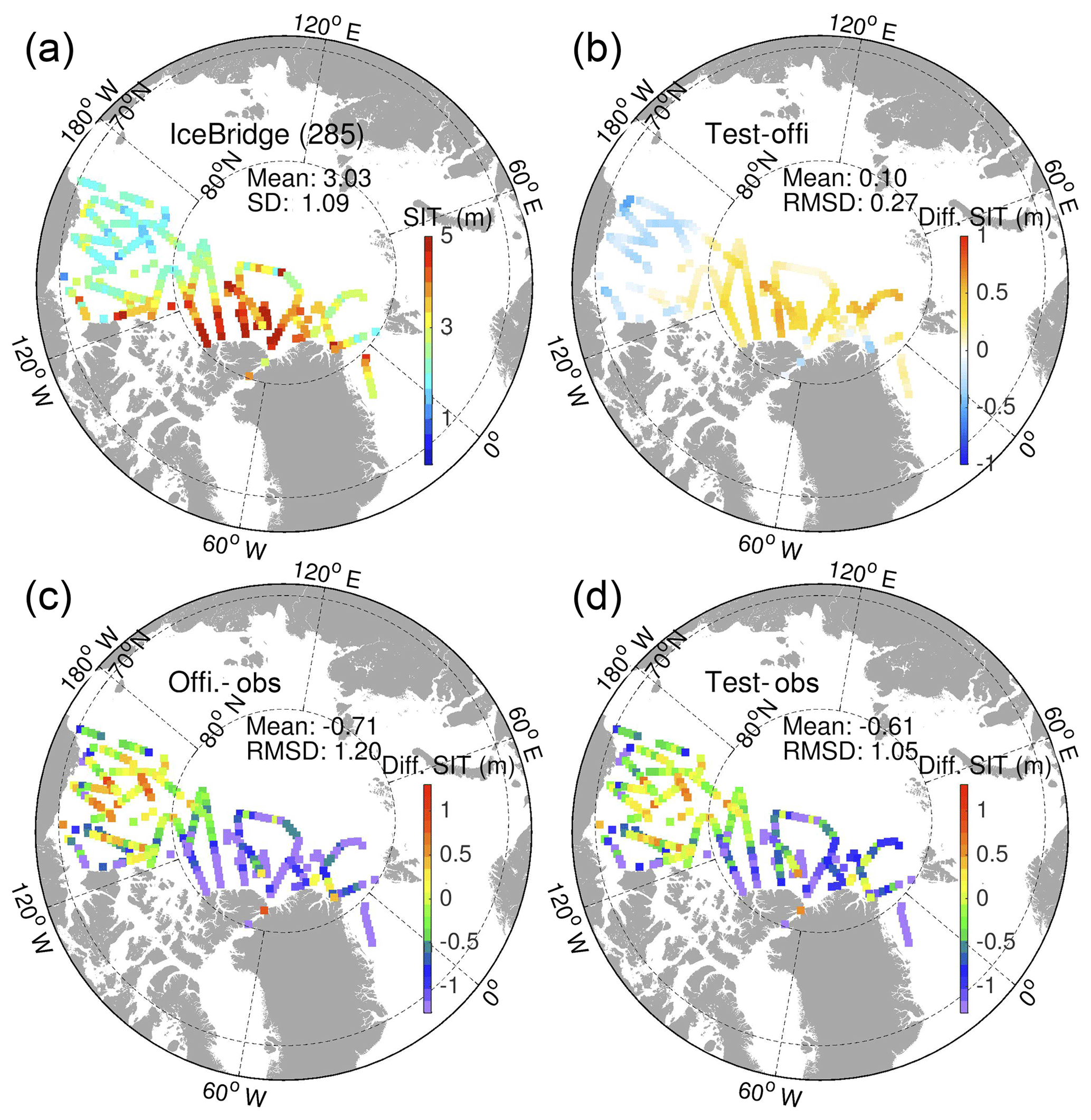
Figure 7(a) IceBridge SIT in 2014 and 2015 and (b) the SIT differences in the two model runs according to the observational locations and times. SIT deviations (c, d) from the Official run (c) and Test run (d) using model daily average at observations time.
The comparisons of the two OSE runs to the IceBridge data are presented in the bottom panels of Fig. 7. The sea ice in the Official run is too thin at the north of the CAA and north of Greenland, with a deviation larger than 1.5 m. In the Beaufort Sea on the contrary, the model is too thick by 0.5 to 1 m. This bias is consistent with that reported in Xie et al. (2017), where the TOPAZ4 reanalysis (Official run) was compared to ICESat observations in the period 2003–2008. In the Test run, the biases are slightly reduced by SIT assimilation, mainly in the Beaufort Sea and north of Greenland, but the reduction is smaller than the remaining error. On average, the SIT RMSD is 1.05 m, which corresponds to a reduction of 12.5 % compared to that in the Official run.
The regression of the SIT observations from IceBridge to the two OSE runs is shown in Fig. 8. The Test run shows improved linear correlations to the observation. The offset at the origin is reduced (0.52 m instead of 0.93 m) and the slope is closer to 1 than in the Official run. The linear correlation in the Test run is slightly increased as indicated with the square correlation R2. There is still a lot of spread which keeps the correlation is on the low side. However, the model still underestimates the thickest ice observed in IceBridge, with a bias as high as 2 m.
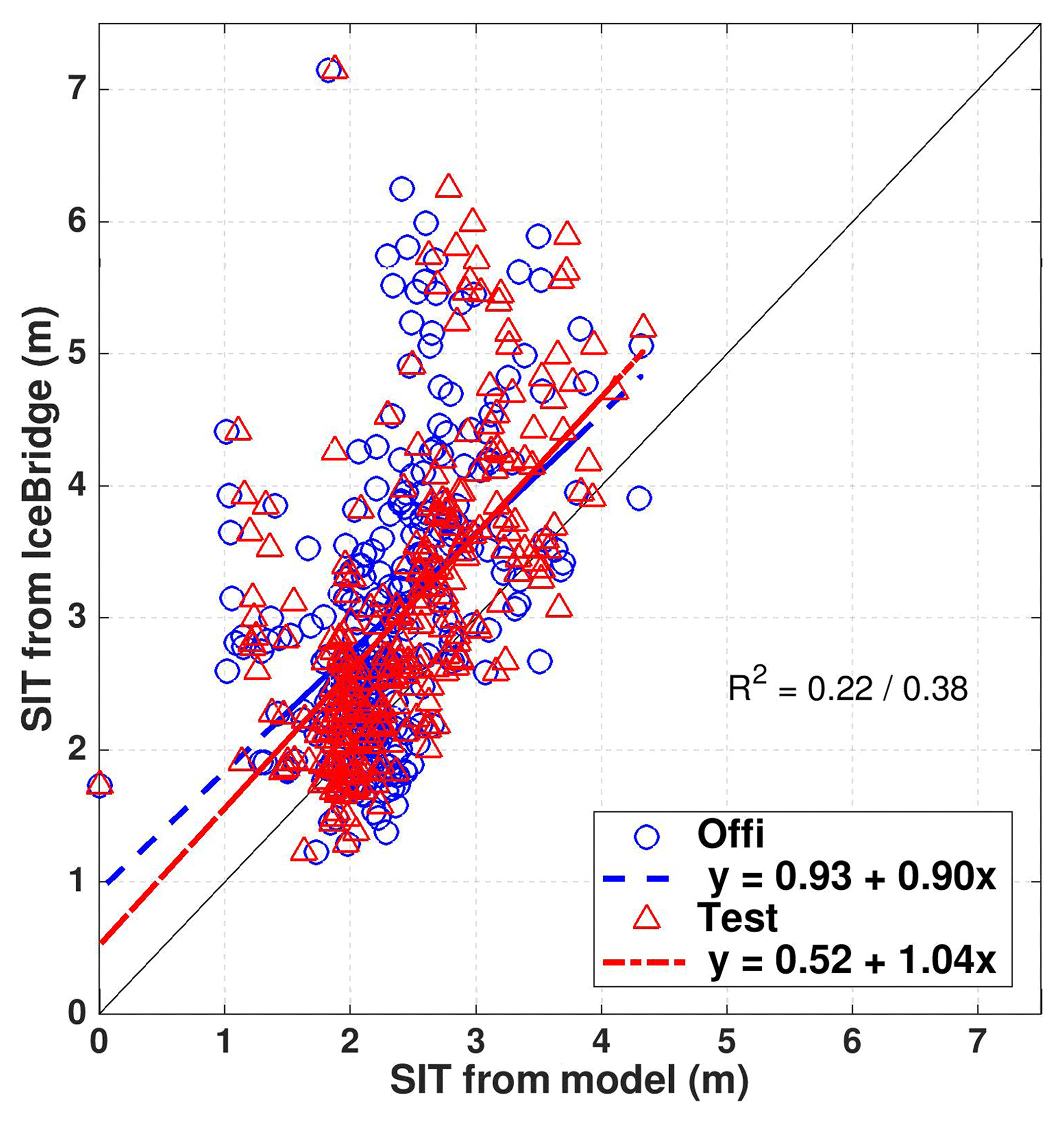
Figure 8Scatterplots of SIT daily averaged of Official (blue) and Test (red) runs compared to IceBridge data. The dashed lines are the respective linear regression, the coefficient R2 is the squared correlation to represent how strong of the linear relationship in Official or Test run. The black line is y=x.
The above results and assimilation diagnostics confirm that the SIT misfits can be controlled – to some degree – by assimilation of the CS2SMOS data, without visible degradation of other assimilated variables. To better understand the advantages and the limits of assimilating the merged SIT product, we further evaluate the impact of CS2SMOS in the assimilation system: first the repercussions on other sea-ice variables and integrated quantities, and then through a quantitative impact analysis of CS2SMOS relatively to other assimilated observation types.
4.1 Impact on the sea-ice drift
The EnKF implemented in TOPAZ4 updates all the variables in the model state vector using flow-dependent multivariate covariances from the ensemble members (Eqs. 1 and 2). The direct assimilation update of ice drift is however short-lived: the ice drift vectors quickly readjust to wind forcing after assimilation, so the ice drift changes are mostly caused by dynamical readjustments, related to the updated ice thickness and ice concentrations. By the first order approximation of the two-dimensional momentum equation (e.g. Hibler III, 1986; Hunke and Dukowicz, 1997), the drift velocity of sea ice is mainly controlled by (1) the interactions of atmosphere–sea ice, (2) the interactions of ocean–sea ice and (3) the internal sea-ice forces which can be represented by the stress tensor σi. The work of Olason and Notz (2014, thereafter called ON14) shows from observations that ice thickness is the main driver changes of ice drift in winter (December to March), while the concentration is the main driver in summer (June to November) and ice drift may increase independently from concentration of thickness in transition periods due to increasing fracturing.
Following the EVP rheology in Hibler III (1979), the stress tensor σi is forced by a pressure term Q which takes a function of the sea-ice thickness and concentration only.
where C0 and P* are empirical constants, dSIT is SIT, and ASIC is sea-ice concentration. ON14 thus show that this type of rheology is able to reproduce the changes of ice drift whenever they are related to changes of concentration and thickness, although not the changes during the transition periods. The sensitivity of ice drift to ice thickness can be directly adjusted by tuning the value of P* in Eq. (10) (see for example Docquier et al., 2017). In the TOPAZ4 model, the sea-ice dynamics assume a viscous-plastic material with an adjustment mechanism at short timescales by elastic waves (called EVP, Hunke and Dukowicz, 1997). The ice thickness does have an influence on the ice concentrations in the summer as well due to melting, but this influence is limited in TOPAZ4 by the assimilation of ice concentrations. The winter months in the seasonal cycle (see Fig. 6 in ON14) indicate that a 10 % increase of ice thickness can reduce the ice drift by 9 %. Areas of thinner ice are much more sensitive (see Fig. 5 in ON14) and therefore the above numbers are subject to possible biases of ice thickness. The sensitivity on seasonal time scales may also differ from the sensitivity on a weekly time scale (that of the TOPAZ4 assimilation cycle).
The evaluation in Xie et al. (2017) shows the model drift of sea ice is overestimated by 2 km d−1 on average on the Arctic with an uncertainty of 5 km d−1. The thickness of thick ice is also too thin, consistently with the too fast drift (Figs. 14 and 17 in Xie et al., 2017). So, the assimilation of ice thickness is expected to improve the ice drift by dynamical model adjustment. Figure 9 shows monthly differences of the 2-day sea-ice drift (SID) compared to the OSI-SAF estimates based on passive microwave data in April 2014, December 2014 and February 2015. The SID in the Official run is too fast in the Central Arctic where the SIT was found too thin in Fig. 3. Despite of the relatively small assimilation impact of CS2SMOS on the SID, there are improvements across the Arctic in all winter months.
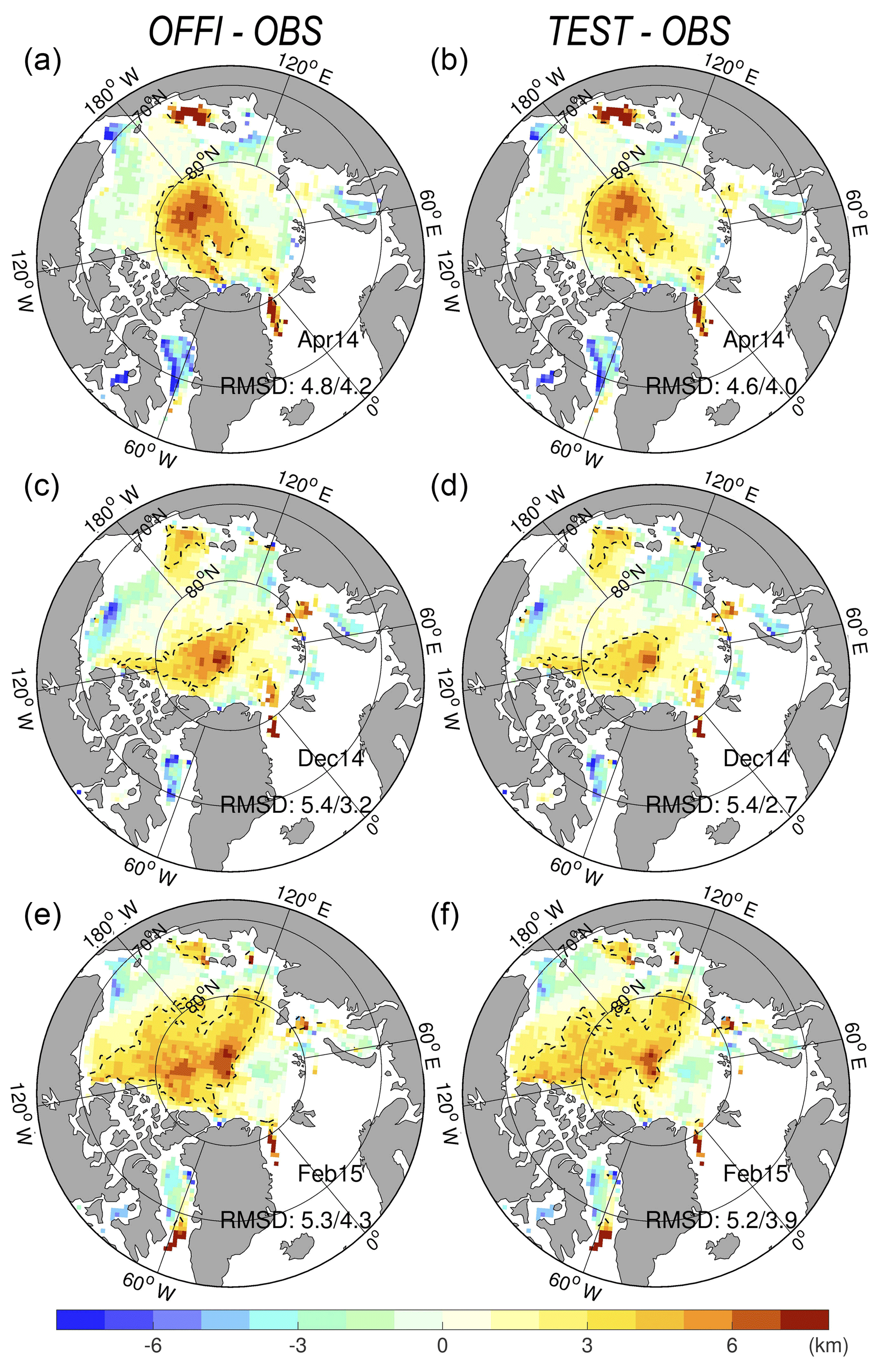
Figure 9Sea-ice drift misfits (model minus observation, in km per 2 days) in the Official run (a, c, e) and Test run (b, d, f), compared against the OSI-SAF sea-ice drift in April 2014 (a, b), December 2014 (c, d) and February 2015 (e, f). The black dashed line delimits the area of fastest drift (drift >3 km per 2 days), and the RMSD relative to the monthly observations is indicated when calculated for the whole domain and at for the region north of 80∘ N.
The RMSD of sea-ice drift speed in 2-day trajectories is reduced by about 0.1–0.2 km in April 2014 and February 2015 for the whole Arctic, which corresponds to a reduction of less than 5 % of the RMSD. However, near the North Pole (north of 80∘ N), the reduction of drift RMSDs is more important, by about 0.4–0.5 km. In December 2014 and February 2015, they have about 8 %–9 % of the error in the Official run. Near the North Pole the averaged SIT in March 2015 (Fig. 3) is about 10 % thicker in the Test run than in the Official run. The impact is more important there than in the rest of the Arctic and well in line with the sensitivity found in ON14. Additionally, there is a small reduction of the fast SID bias but in the case of TOPAZ4, such biases are dependent on the tuning of the drag coefficients between sea ice and the air or the ocean, which has been optimized for the SIT distribution of the TOPAZ free run. The tuning of the drag coefficient adopted by Rampal et al. (2016) is independent from SIT values since it only uses free-drifting ice for tuning.
To evaluate the potential impact of assimilating the SIT from CS2SMOS on the sea-ice motion, we further utilize the data set from the IABP buoys which began in 1990s to monitor ice motion throughout the Arctic Ocean. Only trajectories longer than 30 days and reporting more than 5 times per day are used to estimate the daily drift speed of sea ice. To avoid buoys in open water, the observations are selected based on sea-ice concentration (>0.15) and ice thickness (>5 cm) at the nearest model grid cell in both runs. Furthermore, the data set is restricted in the Central Arctic, (delimited by a red line in Fig. 1b), where water is deeper than 30 m and further away from the coast than 50 km. A total of 151 buoys are left from this selection, which provide 21 793 daily estimates of drift speed.
The speed distribution for daily drift of sea ice from IABP is shown by a histogram in Fig. 10a. In the Central Arctic, the averaged drift speed is about 10.6 km d−1 (consistently with Allard et al., 2018) and most speeds (95 %) are slower than 24 km d−1. The difference of drift distributions between the two runs is minor compared to the difference to the IABP data. Restricting the analysis to the area north of 80∘, the two runs show larger differences in SIT with a Test run about 30 cm thicker (Fig. 10d), the resulting difference in SID in that area is small (0.2 km d−1) and tends to degrade slightly the performance by slowing down the drift speed (Fig. 10c). This is somewhat contradictory to the analysis with OSI-SAF data which indicated a too fast model drift and smaller errors in the Test run. This inconsistency may be due to the poor spatial coverage of the IABP buoys. In Fig. 1 we can see that buoys north of 80∘ N are mainly found in the Eurasian Basin and sample poorly the region between the Transpolar Drift Stream and the Beaufort Gyre (Sumata et al., 2014), where the SID misfits are largest and where the model drift is too fast. This poor coverage of IABP buoys may explain why the SID comparisons in Allard et al. (2018) were inconclusive as well.
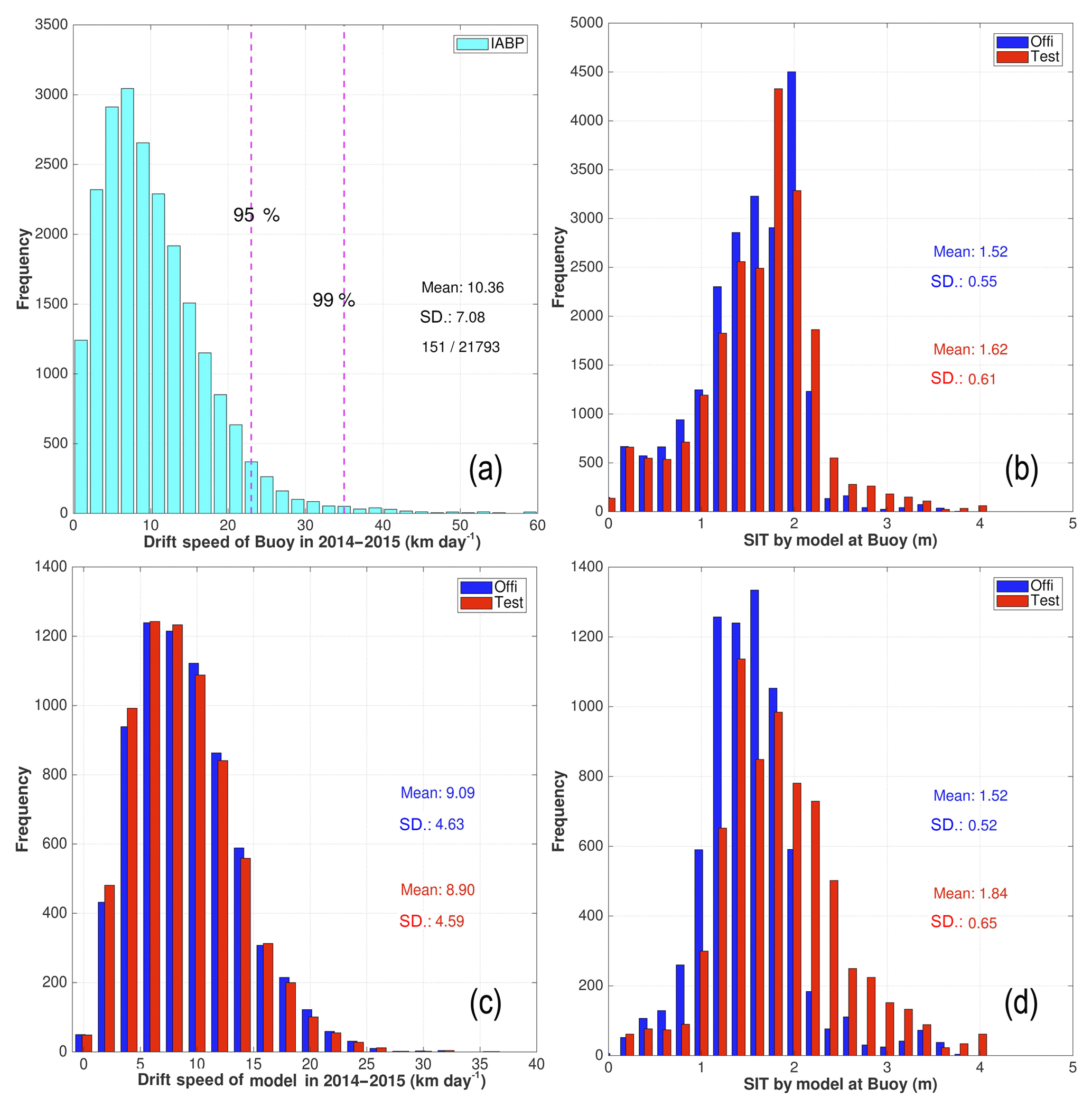
Figure 10(a) Histogram of sea-ice drift speeds calculated from IABP buoys in the Central Arctic for the period 2014–2015. (b) histogram of the simulated SIT at buoys locations in the Central Arctic from the two runs. (c) histogram of the drift speed restricted near the North Pole (>80∘ N) in the Official (blue) and Test (red) runs; the mean speed and the standard deviation are indicated; (d) histogram of the simulated SIT near the North Pole from the two runs.
4.2 Impact on the sea-ice extent and volume in the Central Arctic
In Fig. 3, we show that the Arctic SIT has been improved everywhere, the assessment of the sea-ice drift is less conclusive but tends to suggest a slight improvement localized in the Central Arctic. However, improving the quantitative match with available observations does necessarily warrant the physical consistency of basin-scale integrated quantities. The impact of CS2SMOS on the Arctic-wide sea-ice extent (SIE) and the sea-ice volume (SIV) are investigated for the two runs and compared with the estimates from CS2SMOS and OSI-SAF, respectively. Due to differences of resolution and land mask (especially important in the Canadian Archipelago), we focus on the Central Arctic domain shown as the red line in Fig. 1b, excluding parts of the marginal seas.
Figure 11 shows the time evolutions of SIE and SIV in the two Official and Test runs. Both are calculated by daily averages in the two model runs. The SIE is classically calculated in the area where the SIC is not less than 15 % in the Central Arctic. The SIE shows the expected seasonal cycle with the minimum (close to 3×10⁶ km2) in September 2014 and saturates at a maximum value corresponding to the area of the Central Arctic region (around 6×10⁶ km2) from January to March. The timing of the minimum and maximum from the two model runs agree very well with the observed in OSI-SAF and CS2SMOS (using the weekly concentration from the CS2SMOS product). We can also notice the impact of the weekly assimilation cycle that causes some “sawtooth” discontinuity and indicates that the model tends to both melt too fast in August and freeze too fast in September–October. Overall the SIE differences between the two runs (about 8000 km2) are indiscernible during the experimental time period.

Figure 11SIE and SIV in the official run (blue) and the test run (red) in the Central Arctic. The black stars are the corresponding weekly SIE (or SIV) estimated from CS2SMOS. The green dashed line is the daily SIE from OSI-SAF. The averaged differences of the two runs (Official–Test) are reported. The vertical cyan dashes delimits the periods when C2SMOS data is assimilated.
The time evolutions of the SIV in the two runs show larger differences in the lower panel of Fig. 11. The maximum in the Test run is close to 12×103 km3 in April–May of 2014 and again end of March 2015, and the minimum is close to 5×10³ km3 in September 2014. On average, the SIV difference in the two OSE runs is about 1000 km3, with lower volume in the Official run. Assimilation of the CS2SMOS data yields an annual increase of the SIV by about 8 % relative to that in the Official run. The signature of the assimilation cycle is generally less pronounced than on SIE, except in August 2014 due to the SIC updates that are positively correlated to SIT in the summer (as noted in Lisæter et al., 2003). Compared to the observed SIV from the weekly CS2SMOS, the underestimation is significant at beginning of the runs (about 3×10³ km3), but corrected by one third through the first month of assimilation of CS2SMOS. When the CS2SMOS data are missing, the gap between the two runs remains constant throughout the summer due to the long memory of winter ice, as previously noted with the assimilation work of ICESat SIT data in Mathiot et al. (2012). After the end of the summer during which no data of CS2SMOS are available, the SIV from the Test run is in better agreement with the first observed SIV from CS2SMOS. This indicates that the TOPAZ4 Official run has underestimated SIV due to the history of the reanalysis but not as a systematic tendency towards a bias state. The SIV estimates from observations occasionally present sudden discontinuities that seem unrealistic for a large integrated quantity such as the SIV of the Central Arctic area. These discontinuities are larger than what the data assimilation system would expect based on the assumed observation error statistics given above. But the time series indicate that the EnKF does, as the name indicates, filter out part of the discontinuities so that only the major spike in early November 2014 causes a discontinuity in the Test run. Figure 12 shows that the spike corresponds to a large homogeneous increase of SIT in all marginal seas between 26 October and 2 November 2014, followed by a large decrease in the subsequent week. The weekly SIT innovation on the 2 November reveals that the increase is largest south of the Eurasian Basin and around the Fram Strait. There, the SIT is thinner than 0.3 m on the 26 October which may suggest that the problem comes from the SIT measurement from SMOS. Until such inconsistencies are resolved in the data set, we would recommend to either discard the first weeks of observations or increase the observation error during that period.

Figure 12(a) First three weekly SITs (20–26 October; 27 October–2 November; 3–9 November) from CS2SMOS in the beginning of fall 2014. The dashed white lines denote the 1, 2, 3 and 4 m isolines. (b) The associated time increments of SIT relative to the last weekly SIT. The dashed isolines denote ±1 m.
4.3 Quantitative impact for the observational network
The value of the degrees of freedom for signal (DFS) is commonly used to monitor the relative impact of different observations in a data assimilation system (ref. Cardinali et al., 2004; Rodgers 2000; Xie et al., 2018), and is calculated as follows:
where is the analyzed observation vector, the observation operator H is same in Eq. (1), and the term tr is the trace operator. The DFS is easily calculated and stored while performing the analysis with ensemble data assimilation (see Sakov et al., 2012 for an application to the TOPAZ4 system with the EnKF). It measures the reduction of uncertainty caused by a given observation type expressed as a number of equivalent degrees of freedom. Note that the DFS depend on the observation error statistics but not on the actual observation values (see Eq. 11). A DFS of 0 indicates that the observation has no impact at all, and a DFS equals to the total number of degrees of freedom indicates that the observation has so much impact that it has collapsed the ensemble to a single value. As the analysis is solved either in observational space or in ensemble space (depending on which is computationally cheapest), the DFS cannot exceed the smaller of the ensemble size and the number of observations used for the local assimilation. The DFS quantity is linear and can be split by observation types and accumulated in time periods. The averaged DFS for the kth type of observation can then be noted by , and thus a corresponding impact factor (IF) is defined as:
where O represents the number of different observation types assimilated in this time period. IFk represents the relative impact of the kth type of observations with respect to the whole observation network.
Figures 13 and 14 show the IFk for different observations assimilated in the Test run averaged in 2 typical months: in November 2014 and in March 2015. The SIC impacts are dominant close to the sea-ice edge and in the CAA region in the November, with an average IF of 22.7 % in the whole Arctic. The SIT impact from CS2SMOS is largest in the Central Arctic in November 2014. A relatively smaller impact (>20 %) is also noticeable in north of the Barents Sea and west of the Kara Sea. In the open ocean, the SST and SLA have the largest impact. Temperature and salinity profiles have locally an important effect in the ice-covered Arctic, where a few of ice-tethered profilers (ITP) are available and the uncertainty is large. Xie et al. (2016) applied the same DFS method to evaluate the impact of thin SIT from SMOS only. The present results reveal, as expected, much larger impacts of CS2SMOS SITs in the Central Arctic, with only a few isolated dips where the ITP profiles are available. The IF is higher where the ice is thicker, even though the observation error increases as a function of ice thickness. It indicates that the ensemble background errors increase even more than the observation errors in thick ice by temporal accumulation of model errors. For example, errors in precipitation grow as the snow accumulates in the Fall, and the resulting inter-member variability of snow cover causes inter-member variability of SIT due to the thermal isolation effect of snow.

Figure 13Relative DFS contributions (IF) of each observation data types in November 2014. (a) SIC from OSI-SAF; (b) SIT from CS2SMOS; (c) temperature profiles; (d) salinity profiles; (e) SST; (f) along-track sea level anomaly (SLA). The black line is the 20 % isoline, and the monthly IF (see Eq. 12) is reported between parentheses.
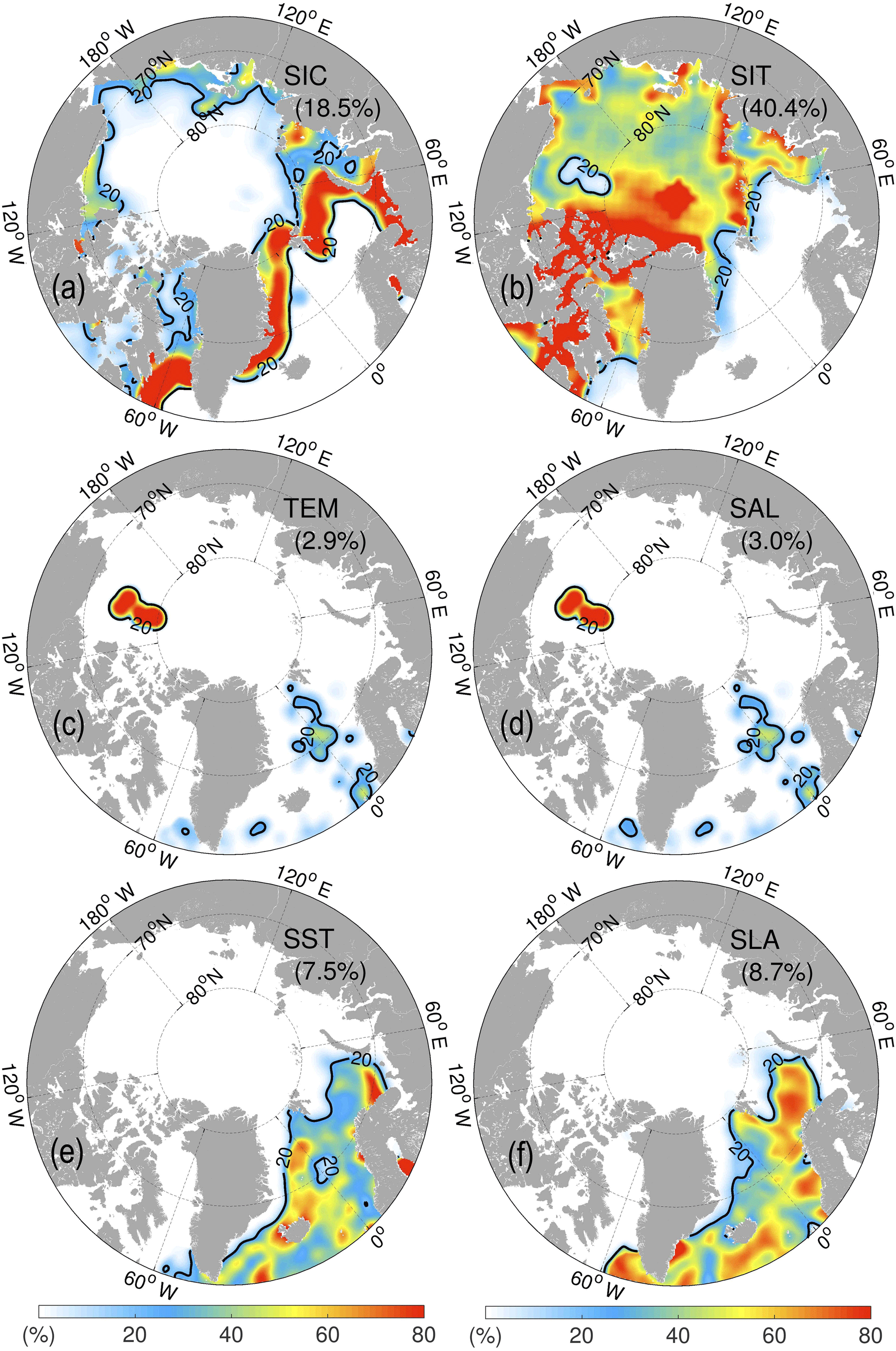
In March 2015, CS2SMOS has again a large impact in the Central Arctic relative to other assimilated observations even though previous literature indicates a lower impact in the midst of winter than when the ice is growing (Mathiot et al., 2012). The relative IF of SIT indeed remains high even though the absolute DFS is decreasing, due to the lower impact of other assimilated observations, in particular SIC (Lisæter et al., 2003). On average, the IF value of CS2SMOS is about 40 %. The high values (>40 %) are clearly separated into two areas: one is to the north of the CAA and Greenland; another following the inner side of the sea-ice edge in marginal ice zones. The former is primarily a CryoSat-2 contribution, while the latter corresponds to the thin SITs from SMOS. The high IF in the polar hole is probably undesirable since the observations there are merely extrapolated, so in the future applications we would recommend discarding these data, in order to leave the polar hole filled instead with sea ice advected from areas where trustworthy SIT observations have been assimilated.
CS2SMOS is the first product to monitor the complete pan-Arctic SIT in a systematic way, although only for the winter months. It is a combination of two very different, yet very advanced, technologies onboard the SMOS and CryoSat-2 satellites, calibrated against very few in situ observations of SIT, freeboard and snow depths. Altogether, the issue of measurements uncertainties is particularly delicate for the assimilation of CS2SMOS data. On the other hand, defining proper model background errors for SIT is just as delicate, when considering that the simulated SIT accumulates errors both in the sea-ice dynamics (in particular the rheological model) and in the thermodynamics. The Bayesian approach to confront these two uncertainties is by Monte Carlo propagation of uncertainties, which is what is practiced in the present study for the model background error, although not for the observation error.
This study assesses the impact of assimilating the new SIT product from 19 March 2014 to 31 March 2015. Compared to the assimilated SIT CS2SMOS, the thin bias is reduced from 15 to 5 cm, and the RMSD also decreased from 58 to 38 cm, a reduction by 28.3 %. Other innovation diagnostics show no degradation towards other assimilated variables – namely SIC, SSH, SST and TS profiles.
The SIT is also improved when compared to four independent drifting IMB buoys and three BGEP mooring buoys. The benefits persist throughout the summer although no SIT observations are available then, consistently with the experiments from Mathiot et al. (2012). This is important because it suggests that the model is not attracted to his bias solution. The assimilation reduces the low SIT biases north of the CAA and north of Greenland and the high bias in the Beaufort Sea compared to independent observations from Operation IceBridge. Both the thick pack ice in Central Arctic and the thin ice in marginal seas are corrected. On average, the SIT errors in March–April of 2014 and 2015 are reduced by 15 cm, a reduction by 12.5 % compared to the Official run.
The dynamical adjustment following the assimilation of SIT has partially improved the sea-ice drift speeds in the Test run where the SIT has thickened: the monthly averaged drift speed errors north of 80∘ N are reduced by 0.4–0.5 km per 2-days in December 2014 and February 2015 (8–9 % reduction of the error). This has been revealed by satellite products but not IABP in situ buoys for which the spatial coverage is very poor. However, it should also be reminded that the drag coefficient used in the Test run were tuned for the Official run which has a biased SIT. One would expect some improvement with a retuned drag coefficient value. At term, we consider doing an online parameter estimation of key parameter such as the drag coefficient as tested in Massonnet et al. (2014).
In this study, the DFS information in the ensemble data assimilation system has been applied to quantitatively evaluate the relative contributions of all assimilated observation types. CS2SMOS has the highest impact near the northern coast of Canada, north of Greenland, and on the inner side of the sea-ice edge, where the contributions from CryoSat-2 and SMOS SIT were expected. The results, compared to assimilating SMOS only in Xie et al. (2016), show the importance of CryoSat-2, particularly in the winter months to constrain the SIT offsets (also shown by Mu et al., 2018, in a coupled MITgcm model system) and motivate the assimilation of CS2SMOS in the following reanalysis of TOPAZ4. However, the impact of SIT observations may vary with the evaluation of the modelling and observing system. Firstly, the SIC may have been underestimated in the Central Arctic due to the simplicity of the present sea-ice model. Further planned developments of TOPAZ include a new model rheology that is able to resolve the scaling laws of deformation of sea ice (Rampal et al., 2016) and should therefore improve the background errors of ice concentration in winter months and sea-ice drift, increase the impact of SIC and SID within the ice pack and reduce the estimated SIT impact accordingly. Other planned changes such as the simulation of melt ponds are not expected to influence these results directly since there are no melt ponds when the SIT data is available. Lastly, if a large number of in situ profiles were available below the sea ice, they would also compete with the SIT observations.
The above OSE results, like others, are necessarily contingent on adequate specifications of observation errors. Those are very much simplified in the case of CS2SMOS, which is not an uncommon case for remote sensing observations: due to the complexity of the physics involved, the specified observation errors are reflecting interpolation errors rather than a nonlinear propagation of errors from their sources (Ricker et al., 2017). In the present study, an offset has been added to account for this difference in Eq. (4), which results in a conservative error estimate with respect to the classical Desroziers optimality criterion and a suboptimal performance in the reliability budget analysis. In the one hand, reducing the observation would have accelerate the convergence to observed SIT and converge to a more accurate solution. On the other hand, this would have made the EnKF less robust to the sudden inconsistencies in the observations as seen in Fig. 11. Further versions of the CS2SMOS data will hopefully improve their temporal continuity and the impact of the data can be increased accordingly.
An alternative to using the scheme CS2SMOS data would have been to assimilate the two data sets CryoSat-2 and SMOS SIT separately and let the EnKF merge them together rather than relying on optimal interpolation, as successfully demonstrated by Mu et al. (2018). This would for instance avoid assimilating observations in places where they are the pure result of interpolation/extrapolation but would not resolve the offset between the two satellites, which is arguably the most worrying issue as of the present state of the SMOS and CryoSat-2 data. The assimilation of the separate data sets will be attempted in the future when their consistency is further improved.
The current TOPAZ reanalysis is currently reaching 2016 and extended by one year every year. The current study clearly shows the added value of assimilating SIT. In 2020, a new TOPAZ reanalysis will be provided with the upgraded version of TOPAZ5 which will include SIT assimilation from 2010 onwards.
The observations used for assimilation and validation are available from the sources mentioned in the text. The Arctic reanalysis after assimilation of CS2SMOS, the Test run, is available from CMEMS (http://marine.copernicus.eu, last access: 22 October 2018) with the product name ARCTIC_REANALYSIS_PHY_002_003, and the Official run is accessible upon request from the authors. The coupled ocean and sea-ice model is available at https://svn.nersc.no/repos/hycom/ (last access: 22 November 2018) and the assimilation code is available at https://svn.nersc.no/enkf/ (last access: 22 November 2018).
JX designed the experiment, performed experiments and analyses. FC and LB contributed to the experimental design and interpretation. JX lead the writing phase, with FC and LB contributing to editing and review.
The authors declare that they have no conflict of interest.
Thanks to Johnny A. Johannessen for discussions and to Stefan Hendricks and
Robert Ricker for sharing the CS2SMOS data on
https://www.meereisportal.de/ (last access: April 2017). Thanks to the
three anonymous reviewers for constructive comments. The authors acknowledge
the support of CMEMS for the Arctic MFC. François Counillon was partly
supported by the NordForsk research program Arctic Climate Predictions:
Pathways to Resilient, Sustainable Societies (ARCPATH, 76654).
Grants of computing time (nn2993k and
nn9481k) and storage (ns2993k) from the Norwegian Sigma2 infrastructures are
also gratefully acknowledged.
Edited by:
Julienne Stroeve
Reviewed by: three anonymous referees
Allard, R. A., Farrell, S. L., Hebert, D. A., Johnston, W. F., Li, L., Kurtz, N. T., Phelps, M. W., Posey, P. G., Tilling, R., Ridout, A., and Wallcraft, A. J.: Utilizing CryoSat-2 sea ice thickness to initialize a coupled ice-ocean modeling system, Adv. Space Res., 62, 1265–1280, https://doi.org/10.1016/j.asr.2017.12.030, 2018.
Bathiany, S., Notz, D., Mauritsen, T., Raedel, G., and Brovkin, V.: On the potential for abrupt Arctic winter sea ice loss. J. Climate, 29, 2703–2719, https://doi.org/10.1175/JCLI-D-15-0466.1, 2016.
Bertino, L. and Lisæter, K. A.: The TOPAZ monitoring and prediction system for the Atlantic and Arctic Oceans, J. Oper. Oceanogr., 1, 15–19, https://doi.org/10.1080/1755876X.2008.11020098, 2008
Bentsen, M., Evensen, G., Drange, H., and Jenkins, A. D.: Coordinate transformation on a sphere using conformal mapping, Mon. Weather Rev., 127, 2733–2740, https://doi.org/10.1175/1520-0493(1999)127<2733:CTOASU>2.0.CO:2, 1999.
Bouillon, S., Fichefet, T., Legat, V., and Madec, G.: The elastic-viscous-plastic method revised, Ocean Modell., 7, 2–12, https://doi.org/10.1016/j.ocemod.2013.05.013, 2013.
Budikova, D.: Role of Arctic sea ice in global atmospheric circulation: A review, Global Planet. Change, 68, 149–163, https://doi.org/10.1016/j.gloplacha.2009.04.001, 2009.
Cardinali, C., Pezzulli, S., and Andersson, E.: Influence-matrix diagnostic of a data assimilation system, Q. J. Roy. Meteor. Soc., 130, 2767–2786, https://doi.org/10.1256/qj.03.205, 2004.
Chassignet, E. P., Smith, L. T., and Halliwell, G. R.: North Atlantic Simulations with the Hybrid Coordinate Ocean Model (HYCOM): Impact of the vertical coordinate choice, reference pressure, and thermobaricity, J. Phys. Oceanogr., 33, 2504–2526, https://doi.org/10.1175/1520-0485(2003)033<2504:NASWTH>2.0.CO:2, 2003.
Comiso, J. C., Parkinson, C. L., Gersten, R., and Stock, L.: Accelerated decline in the Arctic sea ice cover, Geophys. Res. Lett., 35, L01703, https://doi.org/10.1029/2007GL031972, 2008.
Counillon, F. and Bertino, L.: High-resolution ensemble forecasting for the Gulf of Mexico eddies and fronts, Ocean Dynam., 59, 83–95, https://doi.org/10.1007/s10236-008-0167-0, 2009.
Day, J. J., Hawkins, E., and Tietsche S.: Will Arctic sea ice thickness initialization improve seasonal forecast skill?, Geophys. Res. Lett., 41, 7566–7575, https://doi.org/10.1002/2014GL061694, 2014.
Dee, D. P., Uppala, S. M., Simmons, A. J., Berrisford, P., Poli, P., Kobayashi, S., Andrae, U., Balmaseda, M. A., Balsamo, G., Bauer, P., Bechtold, P., Beljaars, A. C. M., van de Berg, I., Biblot, J., Bormann, N., Delsol, C., Dragani, R., Fuentes, M., Greer, A. J., Haimberger, L., Healy, S. B., Hersbach, H., Holm, E. V., Isaksen, L., Kallberg, P., Kohler, M., Matricardi, M., McNally, A. P., Mong-Sanz, B. M., Morcette, J.-J., Park, B.-K., Peubey, C., de Rosnay, P., Tavolato, C., Thepaut, J. N., and Vitart, F.: The ERA-Interim reanalysis: configuration and performance of the data assimilation system, Q. J. Roy. Meteor. Soc., 137, 553–597, https://doi.org/10.1002/qj.828, 2011.
Desroziers, G., Berre, L., and Poli, P.: Diagnosis of observation, background and analysis-error statistics in observation space, Q. J. Roy. Meteor. Soc., 131, 3385–3396, https://doi.org/10.1256/qj.05.108, 2005.
Docquier, D., Massonnet, F., Barthélemy, A., Tandon, N. F., Lecomte, O., and Fichefet, T.: Relationships between Arctic sea ice drift and strength modelled by NEMO-LIM3.6, The Cryosphere, 11, 2829–2846, https://doi.org/10.5194/tc-11-2829-2017, 2017.
Drange, H. and Simonsen, K.: Formulation of air-sea fluxes in the ESOP2 version of MICOM, Technical Report No. 125 of Nansen Environmental and Remote Sensing Center, 1996.
Ferreira, A. S. A., Hátún, H., Counillon, F., Payne, M. R., and Visser, A. W.: Synoptic-scale analysis of mechanisms driving surface chlorophyll dynamics in the North Atlantic, Biogeosciences, 12, 3641–3653, https://doi.org/10.5194/bg-12-3641-2015, 2015.
Finck, N., Counillon, F., Bertino, L., Bouillon, S. and Rampal, P.: Validation of sea ice quantities of TOPAZ for the period 1990-2010, Technical Report No. 332 of Nansen Environmental and Remote Sensing Center, 2013.
Guemas, V., Blanchard-Wrigglesworth, E., Chevallier, M., Day, J. J., Déqué, M., Doblas-Reyes, F. J., Fuckar, N. S., Germe, A., Hawkins, E., Keeley, S., Koenigk, T., Salas y Mélia, D., and Tietsche, S.: A review on Arctic sea-ice predictability and prediction on seasonal to decadal time scales, Q. J. Roy. Meteor. Soc., 142, 546–561, https://doi.org/10.1002/qj.2401, 2014.
Heygster, G., Hendricks, S., Kaleschke, L., Maass, N., Mills, P., Stammer, D., Tonboe, R. T., and Haas, C.: L-Band Radiometry for Sea-Ice Applications, Final Report for ESA ESTEC Contract 21130/08/NL/EL, Institute of Environmental Physics, University of Bremen, 219 pp., available at: http://www.iup.uni-bremen.de/iuppage/psa/documents/smos_final.pdf (last access: 22 November 2018) 2009.
Hibler III, W. D.: A dynamic thermodynamic sea ice model, J. Phys. Oceanogr., 9, 817–846, https://doi.org/10.1175/1520-0485(1979)009<0815:ADTSIM>2.0.CO;2, 1979.
Hibler III, W. D.: Ice dynamics. chap. 9, The Geophysics of Sea Ice, edited by: Untersteiner, N., NATO ASI Series B: Physics, Plenum Press, 577–640, 1986.
Hunke, E. C. and Dukowicz, J. K.: An elastic-viscous-plastic model for sea ice dynamics, J. Phys. Oceanogr., 27, 1849–1867, https://doi.org/10.1175/1520-0485(1997)027<1849:AEVPMF>2.0.CO;2, 1997.
Johannessen, J. A., Raj, R. P., Nilesen, J. E. Ø., Pripp, T., Knudsen, P., Counillon, F., Stammer, D., Bertino, L., Andersen, O. B., Serra, N., and Koldunov, N.: Toward improved estimation of the dynamic topography and ocean circulation in the high latitude and Arctic Ocean: The importance of GOCE, Surv. Geophys., 35, 661–679, https://doi.org/10.1007/s10712-013-9270-y, 2014.
Johannessen, O. M., Shalina, E. V., and Miles, M. W.: Satellite evidence for an Arctic Sea ice cover in transformation, Science, 286, 1937–1939, https://doi.org/10.1126/science.286.5446.1937, 1999.
Johnson, M., Proshutinsky, A., Aksenov, Y., Nguyen, A. T., Lindsay, R., Haas, C., Zhang, J., Diansky, N., Kwok, R., and Maslowski, W.: Evaluation of Arctic sea ice thickness simulated by Arctic Ocean Model Intercomparison Project models, J. Geophys. Res., 117, C00D31, https://doi.org/10.1029/2011JC007257, 2012.
Kaleschke, L., Maaß, N., Haas, C., Hendricks, S., Heygster, G., and Tonboe, R. T.: A sea–ice thickness retrieval model for 1.4 GHz radiometry and application to airborne measurements over low salinity sea-ice, The Cryosphere, 4, 583–592, https://doi.org/10.5194/tc-4-583-2010, 2010.
Kaleschke, L., Tian-Kunze, X., Maaß, N., Ricker, R., Hendricks, S., and Drusch, M.: Improved retrieval of sea ice thickness from SMOS and Cryosat-2. Proceedings of 2015 International Geoscience and Remote Sensing Symposium IGARSS, https://doi.org/10.1109/IGARSS.2015.7327014, 2015.
Karspeck, A. R.: An ensemble approach for the estimation of observational error illustrated for a nominal 1 global ocean model, Mon. Weather Rev., 144, 1713–1728, https://doi.org/10.1175/MWR-D-14-00336.1, 2016.
Kern, S., Khvorostovsky, K., Skourup, H., Rinne, E., Parsakhoo, Z. S., Djepa, V., Wadhams, P., and Sandven, S.: The impact of snow depth, snow density and ice density on sea ice thickness retrieval from satellite radar altimetry: results from the ESA-CCI Sea Ice ECV Project Round Robin Exercise, The Cryosphere, 9, 37–52, https://doi.org/10.5194/tc-9-37-2015, 2015.
Khvorostovsky, K. and Rampal, P.: On retrieving sea ice freeboard from ICESat laser altimeter, The Cryosphere, 10, 2329–2346, https://doi.org/10.5194/tc-10-2329-2016, 2016.
Kimmritz, M., Counillon, F., Bitz, C. M., Massonnet, F., Bethke, I., and Gao, Y.: Optimising assimilation of sea ice concentration in an Earth system model with a multicategory sea ice model., Tellus A, 70, 1435945, https://doi.org/10.1080/16000870.2018.1435945, 2018.
King, J., Howell, S., Derksen, C., Rutter, N., Toose, P., Beckers, J. F., Haas, C., Kurtz, N., and Richter-Menge, J.: Evaluation of Operation IceBridge quick-look snow depth estimates on sea ice, Geophys. Res. Lett., 42, 9302–9310, https://doi.org/10.1002/2015GL066389, 2015.
Kinnard, C., Zdanowicz, C. M., Fisher, D. A., Isaksson, E., Vernal, A., and Thompson, L. G.: Reconstructed changes in Arctic sea ice over the past 1,450 years, Nature, 479, 509–512, https://doi.org/10.1038/nature10581, 2011.
Kwok, R. and Rothrock, D.: Decline in Arctic sea ice thickness from submarine and ICESat records: 1958–2008, Geophys. Res. Lett., 36, L15501, https://doi.org/10.1029/2009GL039035, 2009.
Kurtz, N. T., Farrell, S. L., Studinger, M., Galin, N., Harbeck, J. P., Lindsay, R., Onana, V. D., Panzer, B., and Sonntag, J. G.: Sea ice thickness, freeboard, and snow depth products from Operation IceBridge airborne data, The Cryosphere, 7, 1035–1056, https://doi.org/10.5194/tc-7-1035-2013, 2013.
Laxon, S., Peacock, N., and Smith, D.: High interannual variability of sea ice thickness in the Arctic region, Nature, 425, 947–950, https://doi.org/10.1038/nature02050, 2003.
Lavergne, T., Eastwood, S., Teffah, Z., Schyberg, H., and Breivik, L.-A.: Sea ice motion from low resolution satellite sensors: an alternative method and its validation in the Arctic, J. Geophys. Res., 115, C10032, https://doi.org/10.1029/2009JC005958, 2010.
Levermann, A., Mignot, J., Nawrath, S., and Rahmstorf, S.: The role of Northern sea ice cover for the weakening of the thermohaline circulation under global warming, J. Climate, 20, 4160–4171, https://doi.org/10.1175/JCLI4232.1, 2007.
Lindsay, R. and Schweiger, A.: Arctic sea ice thickness loss determined using subsurface, aircraft, and satellite observations, The Cryosphere, 9, 269–283, https://doi.org/10.5194/tc-9-269-2015, 2015.
Lisæter, K. A., Rosanova, J. J., and Evensen, G.: Assimilation of ice concentration in a coupled ice ocean model, using the Ensemble Kalman filter, Ocean Dynam., 53, 368–388, https://doi.org/10.1007/s10236-003-0049-4, 2003.
Lisæter, K. A., Evensen, G., and Laxon, S.: Assimilating synthetic CryoSat sea ice thickness in a coupled ice-ocean model, J. Geophys. Res., 112, C07023, https://doi.org/10.1029/2006JC003786, 2007.
Martin, S., Drucker, R., Kwok, R., and Holt, B.: Estimation of the thin ice thickness and heat flux for the Chukchi Sea Alaskan coast polynya from Special Sensor Microwave/Imager data, 1990–2001, J. Geophys. Res., 109, C10012, https://doi.org/10.1029/2004JC002428, 2004.
Massonnet, F., Goosse, H., Fichefet, T., and Counillon, F.: Calibration of sea ice dynamic parameters in an ocean-sea ice model using an ensemble Kalman filter, J. Geophys. Res., 119, 4168–4184, https://doi.org/10.1002/2013JC009705, 2014.
Mathiot, P., König Beatty, C., Fichefet, T., Goosse, H., Massonnet, F., and Vancoppenolle, M.: Better constraints on the sea-ice state using global sea-ice data assimilation, Geosci. Model Dev., 5, 1501–1515, https://doi.org/10.5194/gmd-5-1501-2012, 2012.
Melia, N., Haines, K., and Hawkins, E.: Improved Arctic sea ice thickness projections using bias-corrected CMIP5 simulations, The Cryosphere, 9, 2237–2251, https://doi.org/10.5194/tc-9-2237-2015, 2015.
Metzger, E. J., Smedstad, O. M., Thoppil, P. G., Hurlburt, H. E., Cummings, J. A., Wallcraft, A. J., Zamudio, L., Franklin, D. S., Posey, P. G., Phelps, M. W., and Hogan, P. J.: US Navy operational global ocean and Arctic ice prediction systems, Oceanography, 27, 32–43, https://doi.org/10.5670/oceanog.2014.66, 2014.
Mu, L., Yang, Q., Losch, M., Losa, S. N., Ricker, R., Nerger, L., and Liang, X.: Improving sea ice thickness estimates by assimilating CryoSat-2 and SMOS sea ice thickness data simultaneously, Q. J. Roy. Meteor. Soc., 144, 529–538, https://doi.org/10.1002/qj.3225, 2018.
Oke, P. R. and Sakov, P.: Representation error of oceanic observations for data assimilation, J. Atmos. Ocean. Tech., 25, 1004–1017, https://doi.org/10.1175/2007JTECHO558.1, 2008.
Oki, T. and Sud, Y. C.: Design of Total Runoff Integrating Pathways (TRIP) – A Global River Channel Network, Earth Interact., 2, 1–37, https://doi.org/10.1175/1087-3562(1998)002<0001:DOTRIP>2.3.CO;2, 1998.
Olason, E. and Notz, D.: Drivers of variability in Arctic sea-ice drift speed, J. Geophys. Res.-Oceans, 119, 5755–5775, https://doi.org/10.1002/2014JC009897, 2014.
Penny, G., Akella, S. R., Frolov, S., Fujii, Y., Karspeck, A., Peña, M., Subramanian, A., Tardif, R., Wu, X., Anderson, J., Kalnay, E., Kleist, D. T., and Todling, R.: Coupled Data Assimilation for Integrated Earth System Analysis and Prediction: Goals, Challenges, and Recommendations, Technical Report, available at: https://ntrs.nasa.gov/search.jsp?R=20170007430 (last access: 22 November 2018), 2017.
Perovich, D. K. and Richter-Menge, J. A.: From points to Poles: extrapolating point measurements of sea-ice mass balance, Ann. Glaciol., 44, 188–192, https://doi.org/10.3189/172756406781811204, 2006.
Posey, P. G., Metzger, E. J., Wallcraft, A. J., Hebert, D. A., Allard, R. A., Smedstad, O. M., Phelps, M. W., Fetterer, F., Stewart, J. S., Meier, W. N., and Helfrich, S. R.: Improving Arctic sea ice edge forecasts by assimilating high horizontal resolution sea ice concentration data into the US Navy's ice forecast systems, The Cryosphere, 9, 1735–1745, https://doi.org/10.5194/tc-9-1735-2015, 2015.
Rampal, P., Weiss, J., and Marsan, D.: Positive trend in the mean speed and deformation rate of Arctic sea ice, 1979–2007, J. Geophys. Res., 114, C05013 https://doi.org/10.1029/2008JC005066, 2009.
Rampal, P., Bouillon, S., Ólason, E., and Morlighem, M.: neXtSIM: a new Lagrangian sea ice model, The Cryosphere, 10, 1055–1073, https://doi.org/10.5194/tc-10-1055-2016, 2016.
Ricker, R., Hendricks, S., Helm, V., Skourup, H., and Davidson, M.: Sensitivity of CryoSat-2 Arctic sea-ice freeboard and thickness on radar-waveform interpretation, The Cryosphere, 8, 1607–1622, https://doi.org/10.5194/tc-8-1607-2014, 2014.
Ricker, R., Hendricks, S., Kaleschke, L., Tian-Kunze, X., King, J., and Haas, C.: A weekly Arctic sea-ice thickness data record from merged CryoSat-2 and SMOS satellite data, The Cryosphere, 11, 1607–1623, https://doi.org/10.5194/tc-11-1607-2017, 2017.
Rodgers, C.: Inverse methods for atmospheres: theory and practice, World Scientific, 2000.
Rodwell, M. J., Lang, S. T. K., Ingleby, N. B., Bormann, N., Hólm, E., Rabier, F., Richardson, D. S., and Yamaguchi, M.: Reliability in ensemble data assimilation, Q. J. Roy. Meteor. Soc., 142, 443–454, https://doi.org/10.1002/qj.2663, 2016.
Sakov, P. and Oke, P. R.: A deterministic formulation of the ensemble Kalman Filter: an alternative to ensemble square root filters, Tellus A, 60, 361–371, https://doi.org/10.1111/j.1600-0870.2007.00299.x, 2008.
Sakov, P., Counillon, F., Bertino, L., Lisæter, K. A., Oke, P. R., and Korablev, A.: TOPAZ4: an ocean-sea ice data assimilation system for the North Atlantic and Arctic, Ocean Sci., 8, 633–656, https://doi.org/10.5194/os-8-633-2012, 2012.
Schofield, O., Ducklow, H. W., Martinson, D. G., Meredith, M. P., Moline, M. A., and Fraser, W. R.: How Do Polar Marine Ecosystems Respond to Rapid Climate Change?, Science, 5985, 1520–1523, https://doi.org/10.1126/science.1185779, 2011.
Schweiger, A., Lindsay, R., Zhang, J., Steels, M., Stern, H., and Kwok, R.: Uncertainty in modeled Arctic sea ice volume, J. Geophys. Res., 116, C00D06, https://doi.org/10.1029/2011JC007084, 2012.
Smith, G. C., Roy, F., Reszka, M. , Surcel Colan, D., He, Z., Deacu, D., Belanger, J., Skachko, S., Liu, Y., Dupont, F., Lemieux, J., Beaudoin, C., Tranchant, B., Drévillon, M., Garric, G., Testut, C., Lellouche, J., Pellerin, P., Ritchie, H., Lu, Y., Davidson, F., Buehner, M., Caya, A. and Lajoie, M.: Sea ice forecast verification in the Canadian Global Ice Ocean Prediction System, Q. J. Roy. Meteor. Soc., 142, 659–671, https://doi.org/10.1002/qj.2555, 2015.
Stark, J. D., J. Ridley, M. Martin, M., and Hines, A.: Sea ice concentration and motion assimilation in a sea ice–ocean model, J. Geophys. Res., 113, C05S91, https://doi.org/10.1029/2007JC004224, 2008.
Stonebridge, G., Scott, K. A., and Buehner, M.: Impacts on sea ice analyses from the assumption of uncorrelated ice thickness observation errors: Experiments using a 1D toy model, Tellus A, 70, 1445379, https://doi.org/10.1080/16000870.2018.1445379, 2018.
Stroeve, J. C., Serreze, M. C., Holland, M. M., Kay, J. E., Malanik, J., and Barrett, A. P.: The Arctic's rapidly shrinking sea ice cover: a research synthesis, Climatic Change, 10, 1005–1027, https://doi.org/10.1007/s10584-011-0101-1, 2012.
Sumata, H., Lavergne, T., Girard-Ardhuin, F., Kimura, N., Tschudi, M. A., Kauker, F., Karcher, M., and Gerdes, R.: An intercomparison of Arctic ice drift products to deduce uncertainty estimates, J. Geophys. Res.-Oceans, 119, 4887–4921, https://doi.org/10.1002/ 2013JC009724, 2014.
Tian-Kunze, X., Kaleschke, L., Maaß, N., Mäkynen, M., Serra, N., Drusch, M., and Krumpen, T.: SMOS-derived thin sea ice thickness: algorithm baseline, product specifications and initial verification, The Cryosphere, 8, 997–1018, https://doi.org/10.5194/tc-8-997-2014, 2014.
Tilling, R. L., Ridout, A., and Shepherd, A.: Near-real-time Arctic sea ice thickness and volume from CryoSat-2, The Cryosphere, 10, 2003–2012, https://doi.org/10.5194/tc-10-2003-2016, 2016.
Tilling, R. L., Ridout, A., and Sheperd, A.: Estimating Arctic sea ice thickness and volume using CryoSat-2 radar altimeter data, Adv. Space Res., 62, 1203–1225, https://doi.org/10.1016/j.asr.2017.10.051, 2018.
Uotila, P., Goosse, H., Haines, K., Chevallier, M., Barthélemy, A., Bricaud, C., Carton, J., Fučkar, N., Garric, G., Iovino, D., Kauker, F., Korhonen, M., Lien, V. S., Marnela, M., Massonnet, F., Mignac, D., Peterson, A., Sadikn, R., Shi, L., Tietsche, S., Toyoda, T., Xie, J., and Zhang, Z.: An assessment of ten ocean reanalyses in the polar regions, Clim. Dynam., https://doi.org/10.1007/s00382-018-4242-z, online first, 2018.
Wang, Q., Ilicak, M., Gerdes, R., Drange, H., Aksenov, Y., Bailey, D. A., and Yeager, S. G.: An assessment of the Arctic Ocean in a suite of interannual CORE-II simulations. Part I: Sea ice and solid freshwater, Ocean Modell., 99, 110–132, https://doi.org/10.1016/J.OCEMOD.2015.12.008, 2016.
Wang, X., Key, J., Kwok, R., and Zhang, J.: Comparison of Arctic sea ice thickness from satellites, aircraft, and PIOMAS data, Remote Sensing, 8, 1–17, https://doi.org/10.3390/rs8090713, 2016.
Woodgate, R., Aagaard, K., and Weingartner, T.: Monthly temperature, salinity, and transport variability of the Bering Strait through flow, Geophys. Res. Lett., 32, L04601, https://doi.org/10.1029/2004GL021880, 2005.
Xie, J., Bertino, L., Counillon, F., Lisæter, K. A., and Sakov, P.: Quality assessment of the TOPAZ4 reanalysis in the Arctic over the period 1991–2013, Ocean Sci., 13, 123–144, https://doi.org/10.5194/os-13-123-2017, 2017.
Xie, J., Bertino, L., Cardellach, E., Semmling, M., and Wickert, J.: An OSSE evaluation of the GNSS-R altimetery data for the GEROS-ISS mission as a complement to the existing observational networks, Remote Sens. Environ., 209, 152–165, https://doi.org/10.1016/j.rse.2018.02.053, 2018.
Xie, J., Counillon, F., Bertino, L., Tian-Kunze, X., and Kaleschke, L.: Benefits of assimilating thin sea ice thickness from SMOS into the TOPAZ system, The Cryosphere, 10, 2745–2761, https://doi.org/10.5194/tc-10-2745-2016, 2016.
Yang, Q., Losa, S. N., Losch, M., Tian-Kunze, X., Nerger, L., Liu, J., Kaleschke, L., and Zhang, Z.: Assimilating SMOS sea ice thickness into a coupled ice-ocean model using a local SEIK filter, J. Geophys. Res., 119, 6680–6692, https://doi.org/10.1002/2014JC009963, 2014.