Interannual snow accumulation variability on glaciers derived from repeat, spatially extensive ground-penetrating radar surveys

There is significant uncertainty regarding the spatiotemporal distribution of seasonal snow on glaciers, despite being a fundamental component of glacier mass balance. To address this knowledge gap, we collected repeat, spatially extensive high-frequency ground-penetrating radar (GPR) observations on two glaciers in Alaska during the spring of 5 consecutive years. GPR measurements showed steep snow water equivalent (SWE) elevation gradients at both sites; continental Gulkana Glacier's SWE gradient averaged 115 mm 100 m⁻¹ and maritime Wolverine Glacier's gradient averaged 440 mm 100 m⁻¹ (over > 1000 m). We extrapolated GPR point observations across the glacier surface using terrain parameters derived from digital elevation models as predictor variables in two statistical models (stepwise multivariable linear regression and regression trees). Elevation and proxies for wind redistribution had the greatest explanatory power, and exhibited relatively time-constant coefficients over the study period. Both statistical models yielded comparable estimates of glacier-wide average SWE (1 % average difference at Gulkana, 4 % average difference at Wolverine), although the spatial distributions produced by the models diverged in unsampled regions of the glacier, particularly at Wolverine. In total, six different methods for estimating the glacier-wide winter balance average agreed within ±11 %. We assessed interannual variability in the spatial pattern of snow accumulation predicted by the statistical models using two quantitative metrics. Both glaciers exhibited a high degree of temporal stability, with ∼85 % of the glacier area experiencing less than 25 % normalized absolute variability over this 5-year interval. We found SWE at a sparse network (3 stakes per glacier) of long-term glaciological stake sites to be highly correlated with the GPR-derived glacier-wide average. We estimate that interannual variability in the spatial pattern of winter SWE accumulation is only a small component (4 %–10 % of glacier-wide average) of the total mass balance uncertainty and thus, our findings support the concept that sparse stake networks effectively measure interannual variability in winter balance on glaciers, rather than some temporally varying spatial pattern of snow accumulation.

1 Introduction

Our ability to quantify glacier mass balance is dependent on accurately resolving the spatial and temporal distributions of snow accumulation and snow and ice ablation. Significant advances in our knowledge of ablation processes have improved observational and modeling capacities (Hock, 2005; Huss and Hock, 2015; Fitzpatrick et al., 2017), yet comparable advances in our understanding of the distribution of snow accumulation have not kept pace (Hock et al., 2017). Reasons for this discrepancy are 2-fold: (i) snow accumulation exhibits higher variability than ablation, both in magnitude and length scale, largely due to wind redistribution in the complex high-relief terrain where mountain glaciers are typically found (Kuhn et al., 1995) and (ii) accumulation observations are typically less representative (i.e., one stake in an elevation band of a few 100 m) or less effective than comparable ablation observations (i.e., precipitation gage measuring snowfall vs. radiometer measuring short-wave radiation). This discrepancy presents a significant limitation to process-based understanding of mass balance drivers. Furthermore, a warming climate has already modified – and will continue to modify – the magnitude and spatial distribution of snow on glaciers through a reduction in the fraction of precipitation falling as snow and an increase in rain-on-snow events (McAfee et al., 2013; Klos et al., 2014; McGrath et al., 2017; Beamer et al., 2017; Littell et al., 2018).

Significant research has been conducted on the spatial and, to a lesser degree, the temporal variability of seasonal snow in mountainous and high-latitude landscapes (e.g., Balk and Elder, 2000; Molotch et al., 2005; Erickson et al., 2005; Deems et al., 2008; Sturm and Wagner, 2010; Schirmer et al., 2011; Winstral and Marks, 2014; Anderson et al., 2014; Painter et al., 2016). Although major advances have occurred in applying physically based snow distribution models (i.e., iSnobal, Marks et al., 1999, SnowModel, Liston and Elder, 2006, Alpine 3-D, Lehning et al., 2006), the paucity of required meteorological forcing data proximal to glaciers limits widespread application. Many other studies have successfully developed statistical approaches that rely on the relationship between the distribution of snow water equivalent (SWE) and physically based terrain parameters (also referred to as physiographic or topographic properties or variables) to model the distribution of SWE across entire basins (e.g., Molotch et al., 2005; Anderson et al., 2014; Sold et al., 2013; McGrath et al., 2015).

A major uncertainty identified by these studies is the degree to which these statistically derived relationships remain stationary in time. Many studies (Erickson et al., 2005; Deems et al., 2008; Sturm and Wagner, 2010; Schirmer et al., 2011; Winstral and Marks, 2014; Helfricht et al., 2014) have found “time-stability” in the distribution of SWE, including locations where wind redistribution is a major control on this distribution. For instance, a climatological snow distribution pattern, produced from the mean of nine standardized surveys, accurately predicted the observed snow depth in a subsequent survey in a tundra basin in Alaska (∼4–10 cm root mean square error (RMSE); Sturm and Wagner, 2010). Repeat lidar surveys over two years at three hillslope-scale study plots in the Swiss Alps found a high degree of correlation (r=0.97) in snow depth spatial patterns (Schirmer et al., 2011). They found that the final snow depth distributions at the end of the two winter seasons were more similar than the distributions of any two individual storms during that 2-year period (Schirmer et al., 2011). Lastly, an 11-year study of extensive snow probing (∼1200 point observations) at a 0.36 km² field site in southwestern Idaho found consistent spatial patterns (r=0.84; Winstral and Marks, 2014). Collectively, these studies suggest that in landscapes characterized by complex topography and extensive wind redistribution of snow, spatial patterns are largely time-stable or stationary, as long as the primary drivers are stationary.

Even fewer studies have explicitly examined the question of interannual variability in the context of snow distribution on glaciers. Spatially extensive snow probe datasets are collected by numerous glacier monitoring programs (e.g., Bauder, 2017; Kjøllmoen et al., 2017; Escher-Vetter et al., 2009) in order to calculate a winter mass balance estimate. Although extensive, such manual approaches are still limited by the number of points that can be collected and uncertainties in correctly identifying the summer surface in the accumulation zone, where seasonal snow is underlain by firn. One study of two successive end-of-winter surveys of snow depth using probes on a glacier in Svalbard found strong interannual variability in the spatial distribution of snow, and the relationship between snow distribution and topographic features (Hodgkins et al., 2005). Elevation was found to only explain 38 %–60 % of the variability in snow depth, and in one year, snow depth was not dependent on elevation in the accumulation zone (Hodgkins et al., 2005). Instead, aspect, reflecting relative exposure or shelter from prevailing winds, was found to be a significant predictor of accumulation patterns. In contrast, repeat airborne lidar surveys of a ∼36 km² basin (∼50 % glacier cover) in Austria over five winters found that the glacierized area exhibited less interannual variability (as measured by the interannual standard deviation) than the non-glacierized sectors of the basin (Helfricht et al., 2014). Similarly, a three-year study of snow distribution on Findel Glacier in the Swiss Alps using ground-penetrating radar (GPR) found low interannual variability, as 86 % of the glacier area experienced less than 25 % normalized relative variability (Sold et al., 2016). These latter studies suggest that seasonal snow distribution on glaciers likely exhibits “time-stability” in its distribution, but few datasets exist to robustly test this hypothesis.

The “time-stability” of snow distribution on glaciers has particularly important implications for long-term glacier mass balance programs, as seasonal and annual mass balance solutions are derived from the integration of a limited number of point observations (e.g., 3 to 50 stakes), and the assumption that stake and snow pit observations accurately represent interannual variability in mass balance rather than interannual variability in the spatial patterns of mass balance. Previous work has shown “time-stability” in the spatial pattern of annual mass balance (e.g., Vincent et al., 2017) and while this is important for understanding the uncertainties in glacier-wide mass balance estimates, the relative contributions of accumulation and ablation to this stability are poorly constrained, thereby hindering a process-based understanding of these spatial patterns. Furthermore, accurately quantifying the magnitude and spatial distribution of winter snow accumulation on glaciers is a prerequisite for understanding the water budget of glacierized basins, with direct implications for any potential use of this water, whether that be ecological, agricultural, or human consumption (Kaser et al., 2010).

To better understand the “time-stability” of the spatial pattern of snow accumulation on glaciers, we present 5 consecutive years of extensive GPR observations for two glaciers in Alaska. First, we use these GPR-derived SWE measurements to train two different types of statistical models, which were subsequently used to spatially extrapolate SWE across each glacier's area. Second, we assess the temporal stability in the resulting spatial distribution in SWE. Finally, we compare GPR-derived winter mass balance estimates to traditional glaciological derived mass balance estimates and quantify the uncertainty that interannual variability in spatial patterns in snow accumulation introduces to these estimates.

2 Study area

During the spring seasons of 2013–2017, we conducted GPR surveys on Wolverine and Gulkana glaciers, located on the Kenai Peninsula and eastern Alaskan Range in Alaska (Fig. 1). These glaciers have been studied as part of the U.S. Geological Survey's Benchmark Glacier (USGS) project since 1966 (O'Neel et al., 2014). Both glaciers are ∼16 km² in area and span ∼1200 m in elevation (426–1635 m a.s.l. for Wolverine, 1163–2430 m a.s.l. for Gulkana). Wolverine Glacier exists in a maritime climate, characterized by warm air temperatures (mean annual temperature $=-\mathrm{0.2}$ ^∘C at 990 m; median equilibrium line altitude for 2008–2017 is 1235 m a.s.l.) and high precipitation (median glacier-wide winter balance =2.0 m water equivalent (m w.e.)), while Gulkana is located in a continental climate, characterized by colder air temperatures (mean annual temperature $=-\mathrm{2.8}$ ^∘C at 1480 m; median equilibrium line altitude for 2008–2017 is 1870 m a.s.l.) and less precipitation (median glacier-wide winter balance =1.2 m w.e.) (Fig. 2). The cumulative mass balance time series for both glaciers is negative ($\sim -\mathrm{24}$ m w.e. between 1966–2016), with Gulkana showing a more monotonic decrease over the entire study interval, while Wolverine exhibited near equilibrium balance between 1966 and 1987, and sharply negative to present (O'Neel et al., 2014, 2018).

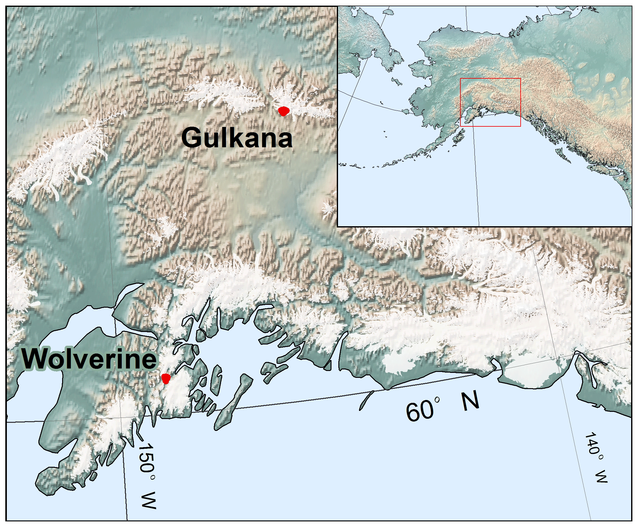
Figure 1 Map of southern Alaska with study glaciers marked by red outline. All glaciers in the region are shown in white (Pfeffer et al., 2014).

3 Methods

The primary SWE observations are derived from a GPR measurement of two-way travel time (twt) through the annual snow accumulation layer. We describe five main steps to convert twt along the survey profiles to annual distributed SWE products for each glacier. These include (i) acquisition of GPR and ground-truth data, (ii) calculation of snow density and associated radar velocity, which are used to convert measured twt to annual layer depth and subsequently SWE, and (iii) application of terrain parameter statistical models to extrapolate SWE across the glacier area. We then describe approaches to (iv) evaluate the temporal consistency in spatial SWE patterns and (v) compare GPR-derived SWE and direct (glaciological) winter mass balances.

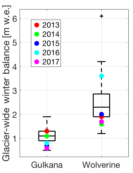
Figure 2 Box plots of glacier-wide winter balance for Gulkana and Wolverine glaciers between 1966 and 2017. Years corresponding to GPR surveys are shown with colored markers. These values have not been adjusted by the geodetic calibration (see O'Neel et al., 2014).

3.1 Radar data collection and processing

Common-offset GPR surveys were conducted with a 500 MHz Sensors and Software pulseEKKO Pro system in late spring close to maximum end-of-winter SWE and prior to the onset of extensive surface melt. GPR parameters were set to a waveform-sampling rate of 0.1 ns, a 200 ns time window, and “Free Run” trace increments, where samples are collected as fast as the processor allows, instead of at uniform temporal or spatial increments.

In general, GPR surveys were conducted by mounting a plastic sled behind a snowmobile and driving at a near-constant velocity of 15 km h⁻¹ (Figs. 3, S1, S2 in the Supplement), resulting in a trace spacing of ∼20 cm. Coincident GPS data were collected using a Novatel Smart-V1 GPS receiver (Omnistar corrected, L1 receiver with root-mean-square accuracy of 0.9 m, Perez-Ruiz et al., 2011). We collected a consistent survey track from year-to-year that minimized safety hazards (crevasses, avalanche runouts) but optimized the sampling of terrain parameter space on the glacier (e.g., range and distribution of elevation, slope, aspect, curvature). However, in 2016 at Wolverine Glacier, weather conditions and logistics did not allow for ground surveys to be completed. Instead, a number of radar lines were collected via a helicopter survey. To best approximate the ground surveys completed in other years, we selected a subset of helicopter GPR observations within 150 m of the ground-based surveys. Previous comparisons between ground and helicopter platforms found excellent agreement in SWE point observations (coefficient of determination (R²)=0.96, RMSE =0.14 m; McGrath et al., 2015).

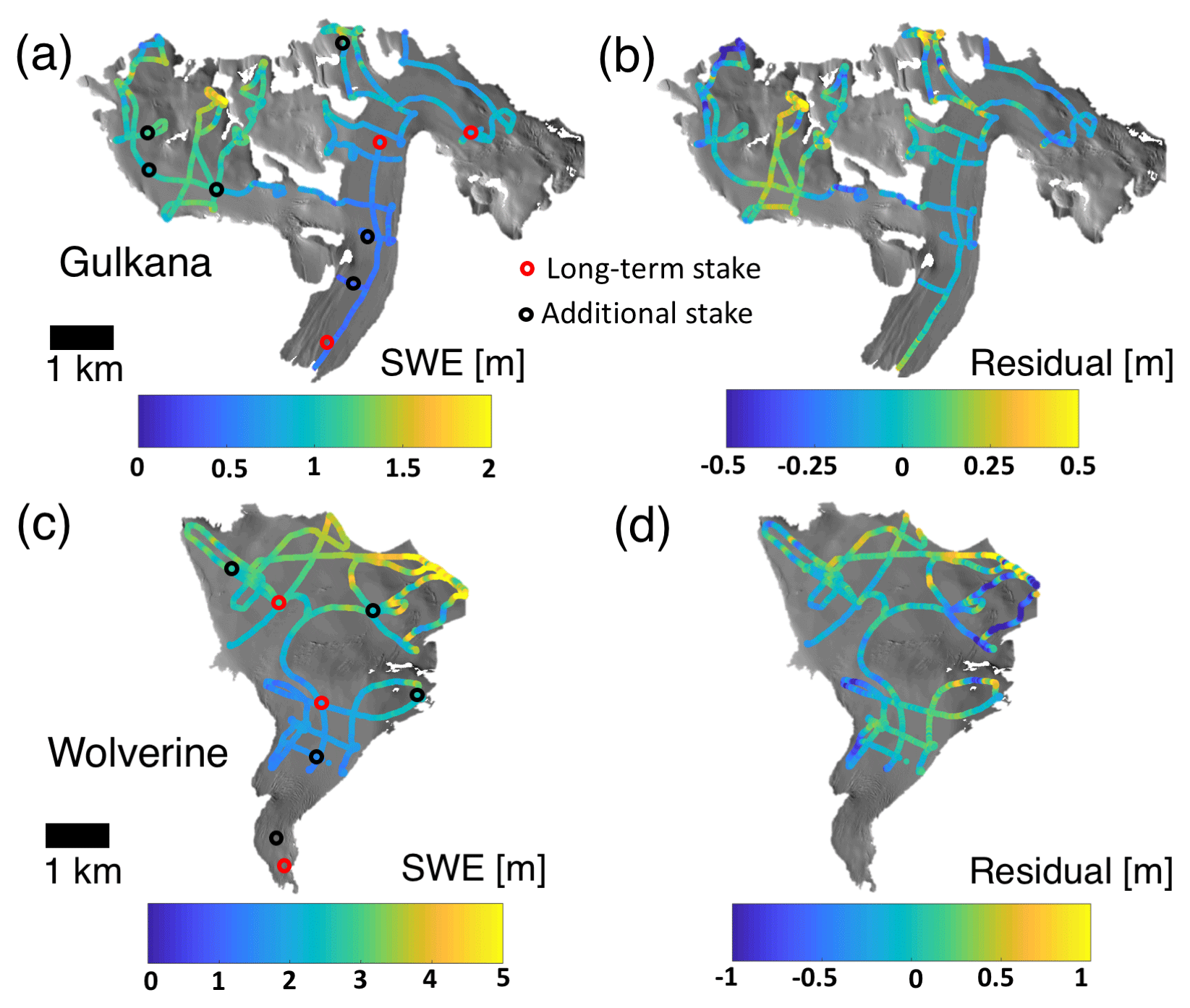
Figure 3 GPR surveys from 2015 at Gulkana (a) and Wolverine (c) glaciers and MVR model residuals (b, d).

Radargrams were processed using the ReflexW-2D software package (Sandmeier Scientific Software). All radargrams were corrected to time zero, taken as the first negative peak in the direct wave (Yelf and Yelf, 2006), and a dewow filter (mean subtraction) was applied over 2 ns. When reflectors from the base of the seasonal snow cover were insufficiently resolved, gain and band-pass filters were subsequently applied. Layer picking was guided by ground-truth efforts and done semi-automatically using a phase-following layer picker. For further details, please see McGrath et al. (2015).

3.2 Ground truth observations

We collected extensive ground-truth data to validate GPR surveys, including probing and snowpits/cores. In the ablation zone of each glacier, we probed the snowpack thickness every ∼500 m along-track. In addition, we measured seasonal snow depth and density at an average of five locations (corresponding to the glaciological observations; see Sect. 3.5) on each glacier in each year. Typically these locations include one or two in the ablation zone, one near the long-term ELA, and two or more in the accumulation zone. We measured snow density using a gravimetric approach in snowpits (at 10 cm intervals) and with 7.25 cm diameter cores (if total depth > 2 m; at 10–40 cm intervals depending on natural breaks) to the previous summer surface. We calculated a density profile and column-average density, ρ_site, at each site.

As snow densities did not exhibit a consistent spatial nor elevation dependency on the glaciers (e.g., Fausto et al., 2018), we calculated a single average density, ρ, of all ρ_site on each glacier and each year, which was subsequently used to calculate SWE:

$$\begin{array}{}\text{(1)}& \mathrm{SWE}=\left({\displaystyle \frac{\mathrm{twt}}{\mathrm{2}}}\right)\cdot v_{\mathrm{s}}\cdot \mathit{\rho },\end{array}$$

where twt is the two-way travel time as measured by the GPR and v_s is the radar velocity. v_s was calculated for each glacier in each year as the average of two independent approaches: (i) an empirical relationship based on the glacier-wide average ρ (Kovacs et al., 1995) and (ii) a least-squares regression between snow depth derived by probing and all radar twt observations within a 3 m radius of the probe site. An exception was made at Wolverine in 2016 as no coincident probe depth observations were made during the helicopter-based surveys. Instead, we estimated the second radar velocity by averaging radar velocities calculated from observed twt and snow depths at three snowpit and core locations.

3.3 Spatial extrapolation

Extrapolating SWE from point measurements to the basin scale has been a topic of focused research for decades (e.g., Woo and Marsh, 1978; Elder et al., 1995; Molotch et al., 2005). Most commonly, the dependent variable SWE is related to a series of explanatory terrain parameters, which are proxies for the physical processes that actually control SWE distribution across the landscape. These include the orographic gradient in precipitation (elevation), wind redistribution of existing snow (slope, curvature, drift potential), and aspect with respect to solar radiation and prevailing winds (eastness, northness). We derived terrain parameters from 10 m resolution digital elevation models (DEMs) sourced from the ArcticDEM project (Noh and Howat, 2015) for Gulkana and produced from airborne structure from motion photogrammetry at Wolverine (Nolan et al., 2015). Both DEMs were based on imagery from August 2015. Specifically, these parameters include elevation, surface slope, surface curvature, northness (Molotch et al., 2005), eastness, and snow drift potential (Sb) (Winstral et al., 2002, 2013; Figs. S3, S4). The Sb parameter is commonly used to identify locations where airflow separation occurs based on both near and far-field topography and are thus likely locations to accumulate snow drifts (Winstral et al., 2002). For specific details on this calculation, please refer to Winstral et al. (2002). In the application of Sb here, we determined the principal direction by calculating the modal daily wind direction during the winter (October–May) when wind speeds exceeded 5 m s⁻¹ (∼ minimum wind velocity for snow transport; Li and Pomeroy, 1997). The length scales for curvature were found using an optimization scheme that identified the highest model R².

Prior to spatial extrapolation, we aggregated GPR observations to the resolution of the DEM by calculating the median value of all observations within each 10 m pixel of the DEM. We then utilized two approaches to extrapolate GPR point observations across the glacier surface: (i) least-squares elevation gradient applied to glacier hypsometry and (ii) statistical models. For (i), we derived SWE elevation gradients in two ways; first, solely on observations that followed the glacier centerline and second, from the entire spatially extensive dataset. For (ii), we utilized two different models: stepwise multivariable linear regressions and regression trees (Breiman et al., 1984). All of these approaches produced a spatially distributed SWE field over the entire glacier area. Individual points in this field are equivalent to point winter balances (b_w; m w.e.). From the distributed b_w field, we calculated a mean area-averaged winter balance (B_w; m w.e.).

Additionally, we implemented a cross-validation approach to the statistical models (multivariable regression and regression tree), whereby 75 % of the aggregated observations were used for training and 25 % were used for testing. However, rather than randomly selecting pixels from across the entire dataset, we randomly selected a single pixel containing aggregated GPR observations and then extended this selection out along continuous survey lines until we reached 25 % of the total observational dataset, thus removing entire sections (and respective terrain parameters) from the analysis (Fig. S5). This approach provided a more realistic test for the statistical models, as the random selection of individual cells did not significantly alter terrain-parameter distributions. For each glacier and each year, we produced 100 training and test dataset combinations, but rather than take the single model with the highest R² or lowest RMSE (between modeled SWE and the GPR-derived test dataset), we produced a distributed SWE product by taking the median value for each pixel from all 100 model runs and a glacier-wide median value that is the median of all 100 individual B_w estimates. We chose the median value approach over a highest R² or lowest RMSE approach that is often utilized because, despite being randomly selected, some training datasets were inherently advantaged by a more complete sampling of terrain parameter distributions. These iterations resulted in the highest R² or lowest RMSE when applied to the training dataset, but were not necessarily indicative of a better model, particularly in the context of being able to predict SWE at locations on the glacier where the terrain parameter space had not been well sampled.

3.3.1 Stepwise multivariable linear regression

We used a stepwise multivariable linear regression model of the form,

$$\begin{array}{}\text{(2)}& {\mathrm{SWE}}_{(i,j)}=c_{\mathrm{1}}{x}_{\mathrm{1}(i,j)}+c_{\mathrm{2}}{x}_{\mathrm{2}(i,j)}+\mathrm{\dots }+c_n{x}_{n(i,j)}+{\mathit{\epsilon }}_{(i,j)},\end{array}$$

where SWE_(i,j) is the predicted (standardized) value at location i,j and $c_{\mathrm{1}},c_{\mathrm{2}},c_n$ are the beta coefficients of the model, $x_{\mathrm{1}},x_{\mathrm{2}},x_n$ are terrain parameters which are independent variables that have been standardized and ε is the residual. We applied the regression model stepwise and included an independent variable if it minimized the Akaike information criterion (AIC; Akaike, 1974). We present the beta coefficients from each regression (each year, each glacier) to explore the temporal stability of these terms.

3.3.2 Regression trees

Regression trees (Breiman et al., 1984) provide an alternative statistical approach for extrapolating point observations by recursively partitioning SWE into progressively more homogenous subsets based on independent terrain parameter predictors (Molotch et al., 2005; Meromy et al., 2013; Bair et al., 2018). The primary advantage of the regression tree approach is that each terrain parameter is used multiple times to partition the observations, thereby allowing for non-linear interactions between these terms. In contrast, the MVR only allows for a single “global” linear relationship for each parameter across the entire parameter-space. We implemented a random forest approach (Breiman, 2001) of repeated regression trees (100 learning cycles) in Matlab, using weak learners and bootstrap aggregating (bagging; Breiman, 1996). Each weak learner omits 37 % of observations, such that these “out-of-bag” observations are used to calculate predictor importance. The use of this ensemble bagging approach reduces overfitting and thus precludes having to subjectively prune the tree and provides more accurate and unbiased error estimates (Breiman, 2001). Prior to implementing the regression tree, we removed the SWE elevation gradient from the observations using a least-squares regression. As described in the results, elevation is the dominant independent variable and as our observations (particularly at Wolverine) did not cover the entire elevation range, the regression tree approach was not well suited to predicting SWE at elevations outside of the observational range.

3.4 Interannual variability in spatial patterns

We quantified the stability of spatial patterns in SWE across the 5-year interval using two approaches: (i) normalized range and (ii) the coefficient of determination. In the first approach, we first divided each pixel in the distributed SWE fields by the glacier-wide average, B_w, for each year and each glacier, and then calculated the range in these normalized values over the entire 5-year interval. For example, if a cell had normalized values of 84 %, 92 %, 106 %, 112 % and 120 %, the normalized range would be 36 %. A limitation of this approach is that it is highly sensitive to outliers, such that a single year can substantially increase this range. This is similar to an approach presented by Sold et al. (2016), but unlike their calculation (their Fig. 9), the normalized values reported here have not been further normalized by the normalized mean of that pixel over the study interval. Thus, the values reported here are an absolute normalized range, whereas Sold et al. (2016) report a relative normalized range. In the coefficient of determination (R²) approach, we computed the least-squares regression correlation between the SWE in each pixel and the glacier-wide average, B_w, derived from the MVR model over the 5-year period. For this approach, cells with a higher R² scale linearly with the glacier-wide average, while those with low R² do not.

3.5 Glaciological mass balance

Beginning in 1966, glacier-wide seasonal (winter, B_w; summer, B_s) and annual balances (B_a) were derived from glaciological measurements made at three fixed locations on each glacier.

The integration of these point measurements was accomplished using a site-index method – equivalent to an area-weighted average (March and Trabant, 1996; van Beusekom et al., 2010). Beginning in 2009, a more extensive stake network of seven to nine stakes was established on each glacier, thereby facilitating the use of a balance profile method for spatial extrapolation (Cogley et al., 2011). Systematic bias in the glaciological mass balance time series is removed via a geodetic adjustment derived from DEM differencing over decadal timescales (e.g., O'Neel et al., 2014). For this study, glaciological measurements were made within a day of the GPR surveys, and integrated over the glacier hypsometry using both the historically applied site-index method (based on the long-term three stake network) and the more commonly applied balance profile method (based on the more extensive stake network). We utilized a single glacier hypsometry, derived from the 2015 DEMs, for each glacier over the entire 5-year interval. Importantly, in order to facilitate a more direct comparison to the GPR-derived B_w estimates, we used glaciological B_w estimates that have not been geodetically calibrated.

4 Results

4.1 General accumulation conditions

Since 1966, Wolverine Glacier's median B_w (determined from the stake network) exceeds Gulkana's by more than a factor of two (2.3 vs. 1.1 m w.e.), and exhibits greater variability, with an interquartile range more than twice as large (0.95 m w.e. vs. 0.4 m w.e.). Over the 5-year study period, both glaciers experienced accumulation conditions that spanned their historical ranges, with one year in the upper quartile (including the fifth greatest B_w at Wolverine in 2016), one year within 25 % of the median, and multiple years in the lower quartile (2017 at Gulkana and 2014 at Wolverine had particularly low B_w values) (Fig. 2). In all years, B_w at Wolverine was greater, although in 2013 and 2014, the difference was only 0.1 m w.e.

Average accumulation season (taken as 1 October–31 May) wind speeds over the study period were stronger (∼7 m s⁻¹ vs. ∼3 m s⁻¹) and from a more consistent direction at Wolverine than Gulkana (northeast at Wolverine, southwest to northeast at Gulkana) (Fig. S6). On average, Wolverine experienced ∼50 days with wind gusts > 15 m s⁻¹ each winter, while for Gulkana, this only occurred on ∼7 days. Over the 5-year study period, interannual variability in wind direction was very low at Wolverine (2016 saw slightly greater variability, with an increase in easterly winds). In contrast, at Gulkana, winds were primarily from the northeast to east in 2013–2015, from the southwest to south in 2016–2017, and experienced much greater variability during any single winter.

Figure 4 SWE from GPR surveys as a function of elevation, along with least squares regression slope and coefficient of determination for each year of the study period. Wolverine is plotted in blue, Gulkana in red.

4.2 In situ and GPR point observations

Glacier-averaged snow densities across all years were 440 kg m⁻³ (range: 414–456 kg m⁻³) at Wolverine and 362 kg m⁻³ (range: 328–380 kg m⁻³) at Gulkana (Table S1 in the Supplement). Average radar velocities were 0.218 m ns⁻¹ (range: 0.207–0.229 m ns⁻¹) at Wolverine and 0.223 m ns⁻¹ (range: 0.211–0.231 m ns⁻¹) at Gulkana. Over this 5-year interval, the GPR point observations revealed a general pattern of increasing SWE with elevation, along with fine-scale variability due to wind redistribution (e.g., upper elevations of Wolverine) and localized avalanche input (e.g., lower west branch of Gulkana) (Figs. S1, S2). The accumulation season (hereafter, winter) SWE elevation gradient was steeper (∼440 vs. ∼115 mm 100 m⁻¹) and more variable in its magnitude at Wolverine than Gulkana. Gradients ranged between 348 and 624 mm 100 m⁻¹ at Wolverine, and 74 and 154 mm 100 m⁻¹ at Gulkana (Fig. 4). Over all 5 years at both glaciers, elevation explained between 50 % and 83 % of the observed variability in SWE (Fig. 4).

4.3 Model performance

To evaluate model performance in unsampled locations of the glacier, both extrapolation approaches were run 100 times for each glacier and each year, each time with a unique, randomly selected training (75 % of aggregated observations) and test (remaining 25 % of aggregated observations) dataset. The median and standard deviation of the coefficients of determination (R²) between modeled SWE and the test datasets for the 100 models runs are shown in Fig. 5. Model performance ranged from 0.25 to 0.75, but on average, across both glaciers and all years, was 0.56 for the MVR approach and 0.46 for the regression tree. Model performance was higher and more consistent at Wolverine, whereas 2015 and 2017 at Gulkana had test dataset R² of ∼0.4 and 0.3, likely reflecting the lower winter SWE elevation gradients and coefficients of determination with elevation during these years (Fig. 4). The wide range in R² across the 100 model runs reflects the variability in training and test datasets that were randomly selected. When the test dataset terrain parameter space was captured by the training dataset, a high coefficient of determination resulted, but when the test dataset terrain parameter space was exclusive (e.g., contained only a small elevation range), the model performance was typically low. This further highlights the importance of elevation as a predictor for these glaciers.

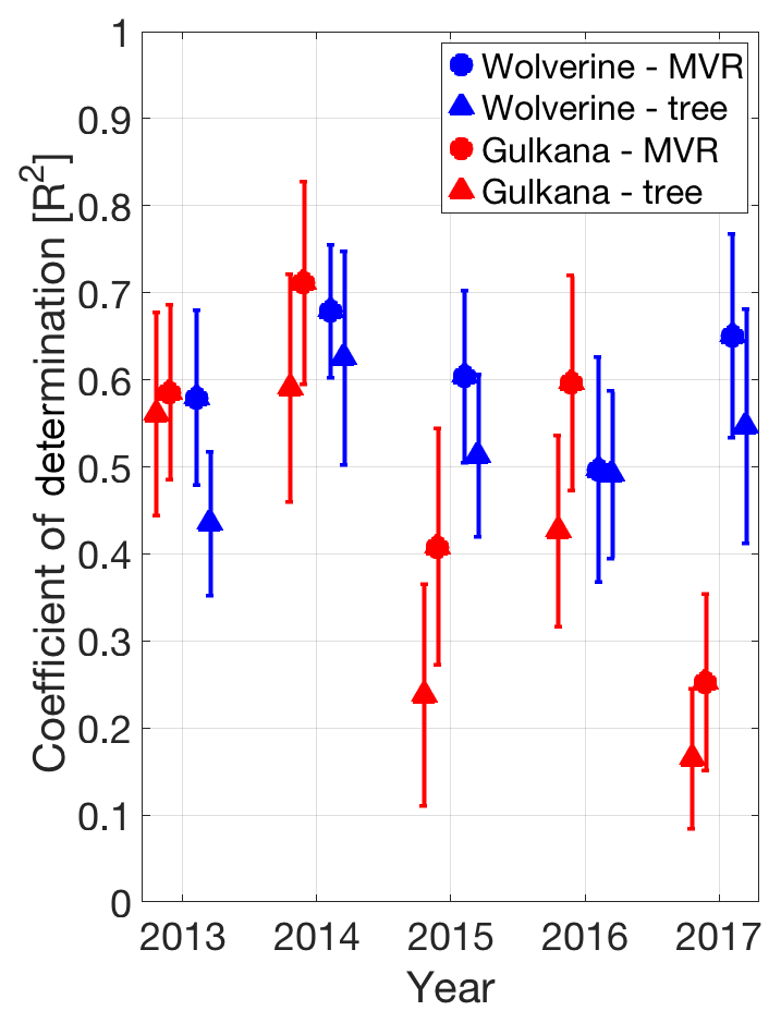
Figure 5 Median and standard deviation (error bars) of coefficient of determination (from 100 model runs) for both extrapolation approaches (circles are MVR, triangles are regression tree) developed on training datasets and applied to test datasets. Symbols and error bars are offset from year for clarity.

At Gulkana, the model residuals (Fig. S1) exhibited spatiotemporal consistency, with positive residuals (i.e., observed SWE exceeded modeled SWE by ∼0.2 m w.e.) at mid-elevations of the west branch and at the very terminus of the glacier. The largest negative residuals typically occurred at the highest elevations. In both cases, these locations deviated from the overall SWE elevation gradient. At Wolverine, observations at the highest elevations typically exceeded the modeled SWE (i.e., positive residuals), particularly at the highest elevations of the northeast corner where wind drifting is particularly prevalent (Fig. S2). For example, in 2015, nearly 80 % of the residuals in this section were positive and had a median value of 0.4 m. Elsewhere at Wolverine, the residuals often alternated between positive and negative values over length scales of 10s to 100s of meters (Fig. S2), which we interpret as zones of scour/drift not captured by the MVR model.

The beta coefficients of terrain parameters from the MVR were fairly consistent from year-to-year at both glaciers (Fig. 6). At Wolverine, elevation was the largest beta coefficient, followed by Sb and curvature. At Gulkana, elevation was also the largest beta coefficient, followed by curvature. Gulkana experiences much greater variability in wind direction during the winter months (Fig. S6), possibly explaining why Sb was either not included or had a very low beta coefficient in the median regression model. As our surveys were completed prior to the onset of ablation, terrain parameters related to solar radiation gain (notably the terms that include aspect: northness and eastness) had small and variable beta coefficients.

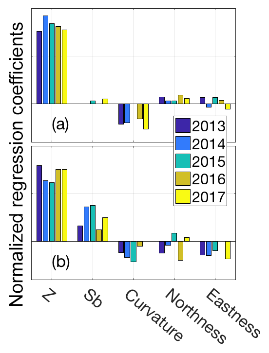
Figure 6 Terrain parameter beta coefficients for (a) Gulkana and (b) Wolverine for multivariable linear regression for each year of the study interval.

4.4 Spatial variability

A common approach for quantifying snow accumulation variability across a range of means is the coefficient of variation (CoV), which is calculated as the ratio of the standard deviation to the mean (Liston et al., 2004; Winstral and Marks, 2014). The mean and standard deviation of CoVs at Wolverine were 0.42±0.03 and at Gulkana, 0.29±0.05, indicating relatively lower spatial variability in SWE at Gulkana (Fig. 7). CoVs were fairly consistent across all 5 years, although 2017 saw the largest CoVs at both glaciers. Interestingly, 2017 had the lowest absolute spatial variability (i.e., lowest standard deviation), but also the lowest glacier-wide averages during the study period, resulting in greater CoVs.

Qualitatively, both Wolverine and Gulkana glaciers exhibited consistent spatiotemporal patterns in accumulation across the glacier surface, with elevation exerting a first-order control (Figs. 8, S7, S8). Overlaid on the strong elevational gradient are consistent locations of wind scour and deposition, reflecting the interaction of wind redistribution and complex – albeit relatively stable year to year – surface topography (consisting of both land and ice topography). For instance, numerous large drifts (∼2 m amplitude, ∼200 m wavelength) occupy the northeast and northwest corners of Wolverine Glacier, where prevailing northeasterly winds consistently redistributed snow into sheltered locations in each year of the study period (Fig. 8). The different statistical extrapolation approaches produced nearly identical B_w estimates (4 % difference on average at Wolverine and 1 % difference on average at Gulkana) (Fig. 9). The MVR B_w estimate was larger in 4 out of 5 years at Wolverine (Fig. 9), while neither approach exhibited a consistent bias at Gulkana.

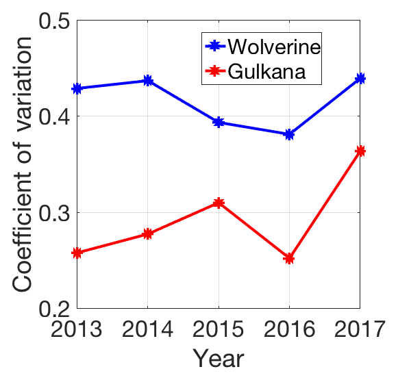
Figure 7 Spatial variability in snow accumulation across the glacier quantified by the coefficient of variation (standard deviation/mean) for each glacier across the 5-year interval based on MVR model output.

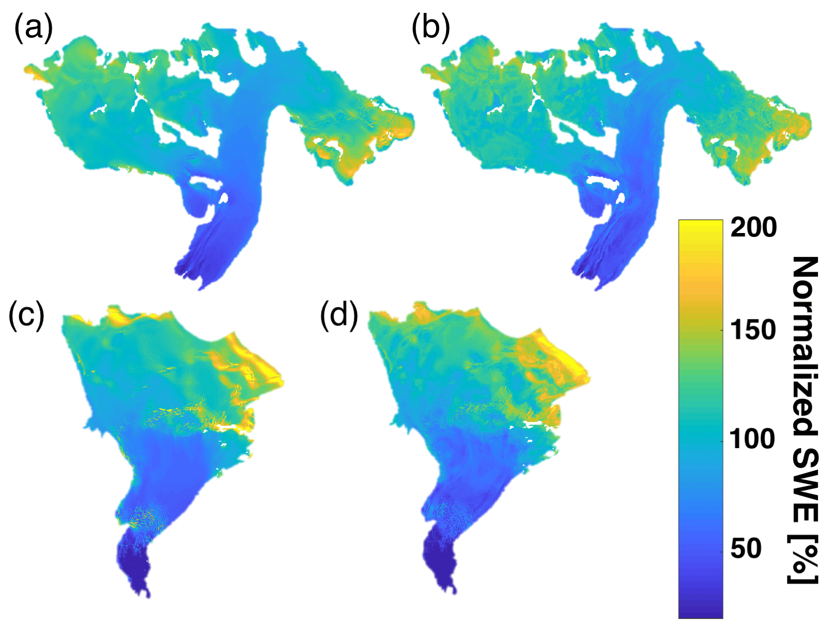
Figure 8 The 5-year mean of normalized distributed SWE for Gulkana (a, b) and Wolverine (c, d) for multivariable regression (a, c) and regression tree (b, d).

Although the glacier-wide averages between these approaches showed close agreement, we explored the differences in spatial patterns by calculating a mean SWE difference map for each glacier by differencing the 5-year mean SWE produced by the regression tree model from the same produced by the MVR model (Fig. 10). As such, locations where the MVR exceeded the regression tree are positive (yellow). At Gulkana, where the two approaches showed slightly better glacier-wide B_w agreement, the magnitude in individual pixel differences were substantially less than at Wolverine (e.g., color bar scales range ±0.2 m at Gulkana vs. ±0.5 m at Wolverine). At Wolverine Glacier, there were three distinct elevation bands where the MVR approach predicted greater SWE, namely the main icefall in the ablation zone, a region of complex topography centered around a normalized elevation of 0.65, and lastly, at higher elevations, where both approaches predicted a series of drift and scour zones, although in sum, the MVR model predicted greater SWE.

We used two different approaches to quantify the “time-stability” of spatial patterns across these glaciers. By the first metric, normalized range, we found that both glaciers exhibited very similar patterns (Fig. 11), with either ∼65 % or 85 % (regression tree and MVR, respectively) of the glacier area experiencing less than 25 % absolute normalized variability (Fig. 12). The R² approach provides an alternative way of assessing the time stability of SWE, essentially determining whether SWE at each location scales with the glacier-wide value. By this metric, 80 % of the glacier area at Wolverine and 96 % of the glacier area at Gulkana (based on MVR model) had a coefficient of determination greater than 0.8 (Fig. 12), suggesting that most locations on the glacier have a consistent relationship with the mean glacier-wide mass balance. By both metrics, the MVR output suggests greater “time-stability” (e.g., lower normalized range or higher R²) compared to the regression tree.

Figure 9 Comparing statistical models for GPR-derived glacier-wide winter balances for both Wolverine (blue) and Gulkana (red) glaciers. For each year and each glacier, two box plots are shown. The first shows multivariable regression model (MVR) output and the second shows regression tree output (tree). The B_w estimate from the glaciological profile method is shown for each year and glacier as the filled circle.

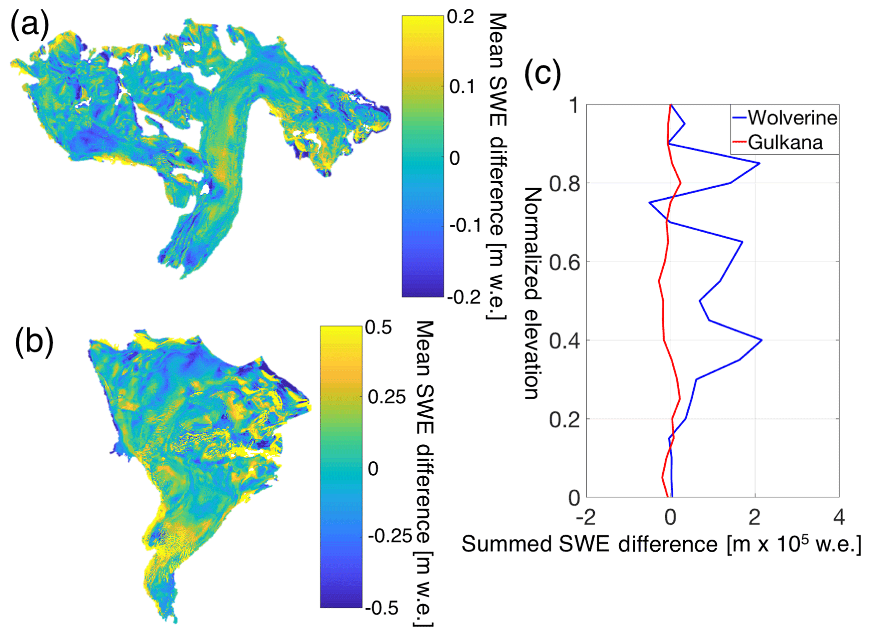
Figure 10 SWE differences between statistical models for Gulkana (a) and Wolverine (b) calculated by differencing the regression tree 5-year mean SWE from the multivariable regression (MVR) 5-year mean SWE. Yellow colors indicate regions where MVR yields more SWE than decision tree and blue colors indicate the opposite. Note different magnitude colorbar scales. (c) Summed SWE difference between methods in bins of 0.05 normalized elevation values.

4.5 Winter mass balance

In order to examine systematic variations between the approaches we outlined in Sect. 3 for calculating the glacier-wide winter balance, B_w,we first calculated a yearly mean from the six approaches (including four based on the GPR observations: MVR, regression tree, elevation gradient derived from centerline only observations, elevation gradient derived from all point observations, and two based on the in situ stake network: site-index and profile). In general, Gulkana exhibited better agreement (4 % average difference) among the approaches, with most approaches agreeing within 5 % of the six-approach mean (Fig. 13; Table S2). Wolverine showed slightly less agreement (7 % average difference), as the two terrain parameters statistical extrapolations (MVR and regression tree) produced B_w estimates ∼9 % above the mean, while the two stake-derived derived estimates were ∼7 % less than the mean. On average across all 5 years at Wolverine, the MVR approach was the most positive, while the glaciological site-index approach was always the most negative (Fig. 13). At both glaciers, the estimates using elevation as the only predictor yielded B_w estimates on average within 3 % of the six-method mean, with the centerline only based estimate being slightly negatively biased, and the complete observations being slightly positively biased.

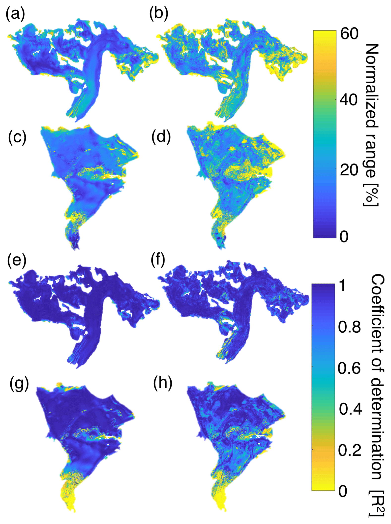
Figure 11 Interannual variability of the SWE accumulation field from 2013–2017, quantified via normalized range (a–d) and R² (e–h) approach for median distributed fields from the multivariable regression (left column) and regression tree (right column) statistical models.

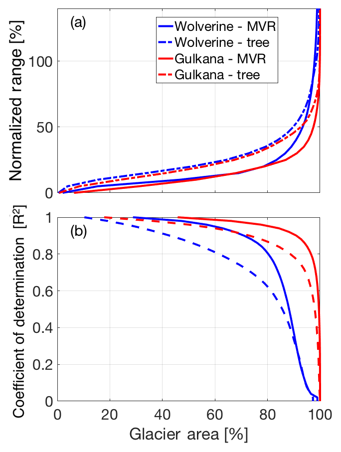
Figure 12 Interannual variability of the SWE accumulation pattern as a function of cumulative glacier area, shown as (a) normalized range and (b) and R². Solid lines are for the multivariable regression (MVR) and dashed lines are for the regression tree.

To examine the systematic difference between the glaciological site-index method and GPR-based MVR approach, we compared stake-derived b_w values from the three long-term stakes to all GPR-based MVR b_w values within that index zone (Fig. 14). Both the stakes and the GPR-derived b_w values have been normalized by the glacier-wide value to make these results comparable across years and glaciers. It is apparent that Wolverine experienced much greater spatial variability in accumulation, with larger interquartile ranges and a large number of positive outliers in all index zones. Importantly, the stake weight in the site-index solution is dependent on the hypsometry of the glacier, and for both glaciers, the upper stake accounts for ∼65 % of the weighted average. In years that the misfit between GPR B_w and site-index B_w was largest (2015 and 2016 at Gulkana, 2013 and 2017 at Wolverine), the stake-derived b_w at the upper stake was in the lower quartile of all GPR-derived b_w values, explaining the significant difference in B_w estimates in these years. Potential reasons for this discrepancy are discussed in Sect. 5.3.

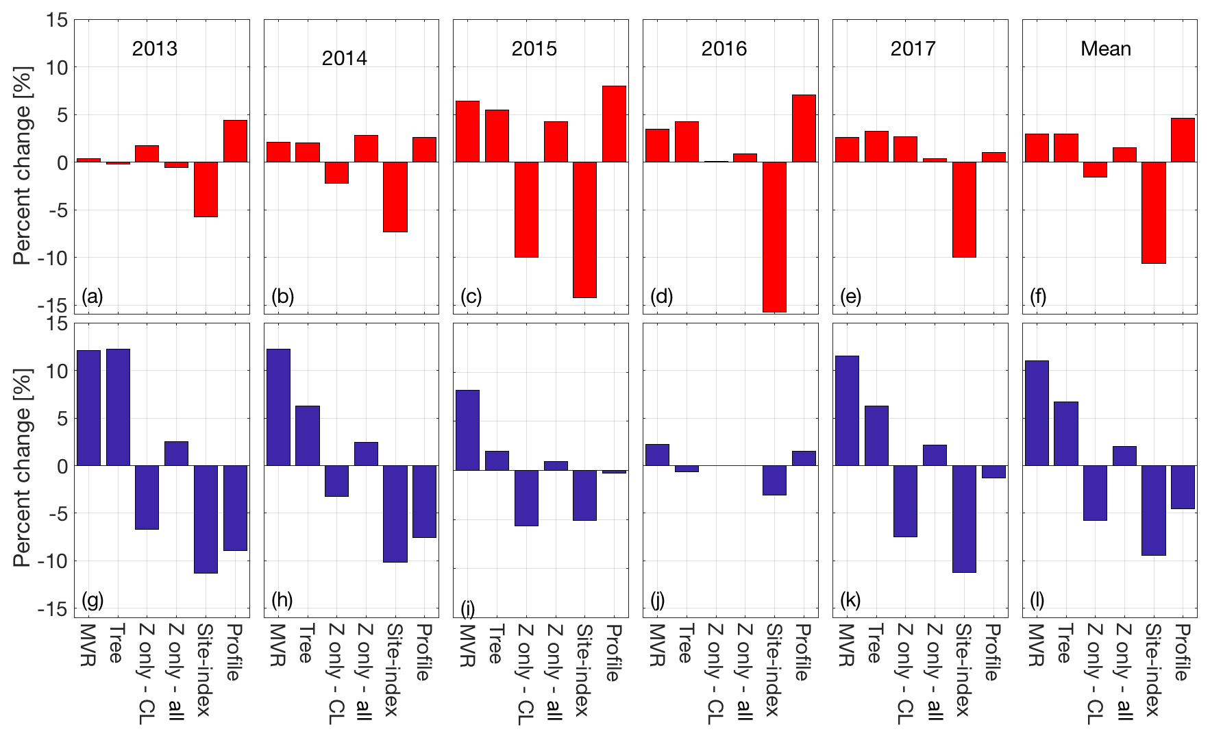
Figure 13 Percent deviation for each estimate from the six-method mean of B_w. Individual years for Gulkana Glacier are shown in panels (a)–(e) with the 5-year mean shown in (f). Individual years for Wolverine Glacier are shown in panels (g)–(k), with the 5-year mean shown in (l).

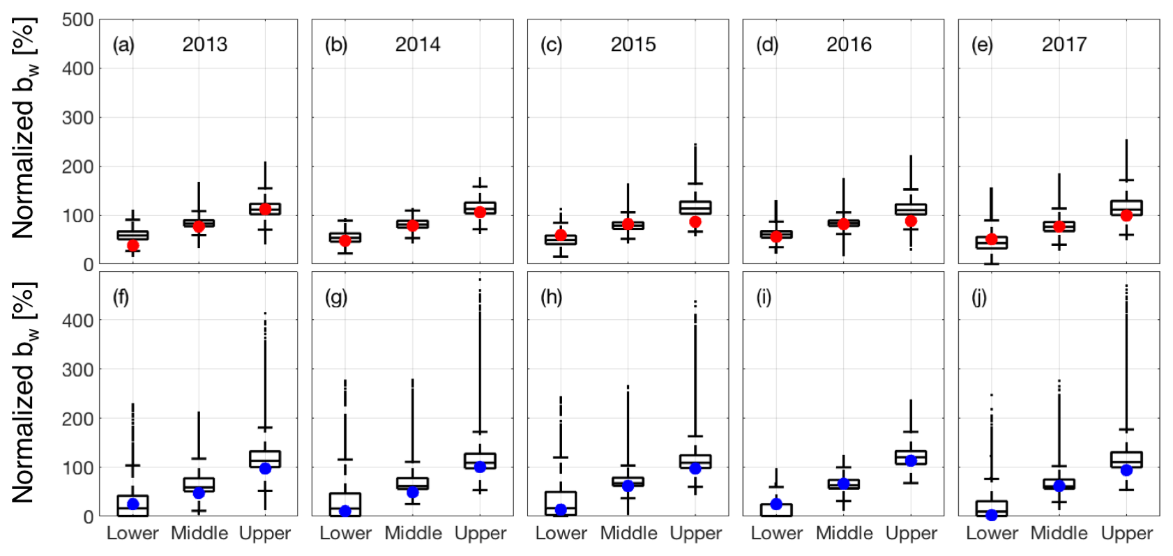
Figure 14 Spatial variability in snow accumulation for individual years (2013–2017) by elevation (lower, middle, upper) compared to stake measurements. Box plot of all distributed SWE values (from multivariable regression) for each index zone of the glacier for Gulkana (a–e) and Wolverine (f–j) for 2013–2017. The filled circles are the respective stake observation for that index zone. SWE is expressed as a percentage of the glacier-wide average, B_w, for that year and glacier.

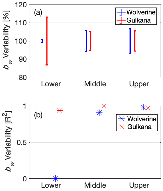
Figure 15 Interannual variability in the spatial pattern of snow accumulation at long-term mass balance stake locations for Wolverine and Gulkana glaciers using (a) normalized b_w range and (b) coefficient of determination (from Fig. 11; MVR model).

In situ stake and pit observations traditionally serve as the primary tool for deriving glaciological mass balances. However, in order for these observations to provide a systematic and meaningful long-term record, they need to record interannual variability in mass balance rather than interannual variability in spatial patterns of mass balance. To assess the performance of the long-term stake sites, we examined the interannual variability metrics for the stake locations. By both metrics (normalized absolute range and R²), the middle and upper elevation stakes at both glaciers appear to be in locations that achieve this temporal stability, having exhibited ∼10 % range and R²> 0.95 over the 5-year interval. The lower elevation stake was less temporally stable and exhibited opposing behavior at each glacier. At Gulkana, this stake had a high R² (0.93) and moderate normalized variability (26 %), which in part, reflects the lower total accumulation at this site and the ability for a single uncharacteristic storm to alter this total amount significantly. In contrast, Wolverine's lowest site exhibited both low R² (< 0.01) and normalized range (2 %), a somewhat unlikely combination. The statistical models commonly predicted zero or near-zero cumulative winter accumulation at this site (i.e., mid-winter rain and/or ablation is common at this site), so although the normalized range was quite low, predicted SWE values were uncorrelated with B_w over the study interval.

5 Discussion

5.1 Interannual variability in spatial patterns

Each glacier exhibited consistent normalized SWE spatial patterns across the 5-year study, reflecting the strong control of elevation and regular patterns in wind redistribution in this complex topography (Figs. 11, S7, S8). This is particularly notable given the highly variable magnitudes of accumulation over the 5-year study and the contrasting climate regions of these two glaciers (wet, warm maritime and cold, dry continental), with unique storm paths, timing of annual accumulation, wind direction and wind direction variability, and snow density. At both glaciers, the lowest interannual variability was found away from locations with complex topography and elevated surface roughness, such as crevassed zones, glacier margins, and areas near peaks and ridges.

In the most directly comparable study, which used repeat GPR surveys on Switzerland's Findel Glacier, 86 % of the glacier area experienced less than 25 % range in relative normalized accumulation over a three-year interval (Sold et al., 2016). As noted in Sect. 3.4., we reported an absolute normalized range, whereas Sold et al. (2016) reported a relative normalized range. Following their calculation, we found that 81 % and 82 % of Wolverine and Gulkana's area experienced a relative normalized range less than 25 %. Collectively, our results add to the growing body of evidence (e.g., Deems et al., 2008; Sturm and Wagner, 2010; Schirmer et al., 2011; Winstral and Marks, 2014) suggesting “time-stability” in the spatial distribution of snow in locations that span a range of climate zones, topographic complexity, and relief. While the initial effort required to constrain the spatial distribution over a given area can be significant, the benefits of understanding the spatial distribution are substantial and long lasting, and have a wide range of applications.

5.1.1 Elevation

Elevation explained between 50 % and 83 % of the observed SWE variability at Gulkana and Wolverine, making it the most significant terrain parameter at both glaciers every year (Figs. 4, 6). Steep winter SWE gradients characterized both glaciers throughout the study period (115–440 mm 100 m⁻¹). Such gradients are comparable to previous results for glaciers in the region (Pelto et al., 2013; McGrath et al., 2015), but exceed reported orographic precipitation gradients in other mountainous regions by a factor of 2–3 (e.g., Anderson et al., 2014; Grünewald and Lehning, 2011). These steep gradients are likely the result of physical processes beyond just orographic precipitation, including storm systems that deliver snow at upper elevations and rain at lower elevations (common at both Wolverine and Gulkana) and mid-winter ablation at lower elevations (at Wolverine). These processes have also been shown to steepen observed SWE gradients relative to orographic precipitation gradients in a mid-latitude seasonal snow watershed (Anderson et al., 2014). Unfortunately, given that we solely sampled snow distribution at the end of the accumulation season, the relative magnitude of each of these secondary processes is not constrained.

Wolverine and Gulkana glaciers exhibited opposing SWE gradients at their highest elevations, with Wolverine showing a sharp non-linear increase in SWE, while Gulkana showed a gradual decrease. This non-linear increase was also noted at two maritime glaciers (Scott and Valdez) in 2013 (McGrath et al., 2015), and perhaps reflects an abundance of split precipitation phase storms in these warm coastal regions. The cause of the observed reverse gradient at Gulkana may be the result of wind scouring at the highest and most exposed sections of the glacier, or in part, a result of where we were able to safely sample the glacier. For instance, in 2013, when we were able to access the highest basin on the glacier, the SWE elevation gradient remained positive (Fig. 4). Reductions in accumulated SWE at the highest elevations have also been observed at Lemon Creek Glacier in southeast Alaska and Findel Glacier in Switzerland (Machguth et al., 2006), presumably related to wind scouring at these exposed elevations.

5.1.2 Wind redistribution

Both statistical extrapolation approaches found terrain parameters Sb and curvature, proxies for wind redistribution, to have the largest beta coefficients after elevation (Figs. 6, S9). The spatial pattern of SWE estimated by each model clearly reflects the dominant influence of wind redistribution and elevation (Fig. 8), as areas of drift and scour are apparent, especially at higher elevations. However, these terms do not fully capture the redistribution process, as the model residuals (Figs. S1, S2) show sequential positive and negative residuals associated with drift and scour zones. There are a number of reasons why this might occur, including variable wind directions transporting snow (this is likely a more significant issue at Gulkana, which experiences greater wind direction variability, Fig. S6), complex wind fields that are not well represented by a singular wind direction (Dadic et al., 2010), changing surface topography (the glacier surface is dynamic over a range of temporal scales, changing through both surface mass balance processes and ice dynamics), and widely varying wind velocities. This is particularly relevant at Wolverine, where wind speeds regularly gust over 30 m s⁻¹ during winter storms, speeds that result in variable length scales of redistribution that would not be captured by a fixed length scale of redistribution. All of these factors influence the redistribution of snow and limit the predictive ability of relatively simple proxies. Significant effort has gone into developing physically based snow-distribution models (e.g., Alpine3D and SnowModel), however, high-resolution meteorological forcing data requirements generally limit the application of these models in glacierized basins. Where such observations do exist, previous studies have illuminated how the final distribution of snow is strongly correlated to the complex wind field, including vertical (surface normal) winds (Dadic et al., 2010).

5.1.3 Differences with non-glaciated terrain

Although our GPR surveys did not regularly include non-glaciated regions of these basins, a few key differences are worth noting. First, the length scales of variability on and off the glacier were distinctly different, with shorter scales and greater absolute variability (snow-free to > 5 m in less than 10 m distance) off glacier (Fig. S10). This point has been clearly shown using airborne lidar in a glaciated catchment in the Austrian Alps (Helfricht et al., 2014). The reduced variability on the glacier is largely due to surface mass balance and ice flow processes that act to smooth the surface, leading to a more spatially consistent surface topography, and therefore a more spatially consistent SWE pattern. For this reason, establishing a SWE elevation gradient on a glacier is likely much less prone to terrain-induced outliers compared to off-glacier sites, although the relationship of this gradient to off-glacier gradients is generally unknown.

5.2 Spatial differences between statistical models

The two statistical extrapolation approaches yielded comparable large-scale spatial distributions and glacier-wide averages, although there were some notable spatial differences (Fig. 10). The systematic positive bias of the MVR approach over the regression tree at Wolverine was due to three sectors of the glacier with both complex terrain (i.e., icefalls) and large data gaps (typically locations that are not safe to access on ground surveys). The difference in predicted SWE in these locations is likely due to how the two statistical extrapolation approaches handle unsampled terrain parameter space. The MVR extrapolates based on global linear trends, while the regression tree assigns SWE from terrain that most closely resembles the under-sampled location. Anecdotally, it appears that the MVR may overestimate SWE in some of these locations, which is most evident in Wolverine's lower icefall, where bare ice is frequently exposed at the end of the accumulation season (Fig. S11) in locations where the MVR predicted substantial SWE. Likewise, the regression tree models could be underestimating SWE in these regions, but in the absence of direct observations the errors are inherently unknown. The regression tree model captures more short length scale variability while the MVR model clarifies the larger trends. Consequently, smaller drifts and scours are captured well by the regression tree model in areas where the terrain parameter space is well surveyed, but the results become progressively less plausible as the terrain becomes distinctly different from the sampled terrain parameter space. In contrast, the MVR model appears to give more plausible results at larger spatial scales. This suggests that there is some theoretical threshold where the regression tree is more appropriate if the terrain parameter space is sampled sufficiently, but that for many glacier surveys the MVR model would be more appropriate.

5.3 Winter mass balance comparisons

On average, all methods for estimating B_w were within ±11 % of the six-method mean (Fig. 13). The agreement (as measured by the average percent difference from the mean) between estimates was slightly better at Gulkana than Wolverine, likely reflecting the overall lower spatial variability at Gulkana and the greater percentage of the glacier area where b_w correlates well with the glacier-wide average (Fig. 11e, f). At both glaciers, B_w solutions based solely on elevation showed excellent agreement to the six-method mean, suggesting that this simple approach is a viable means for measuring B_w on these glaciers.

The biggest differences occurred between the GPR-forced MVR model and the glaciological site-index method, which we have shown is attributed to the upper stake (with the greatest weight) underestimating the median SWE for that index zone (Fig. 14). The upper stake location was established in 1966 at an elevation below the median elevation of that index zone, which given the strong elevation control on SWE, is a likely reason for the observed difference. At Gulkana, the relationship between the upper index site and the GPR-forced MVR model is more variable in large part due to observed differences in the accumulation between the main branch (containing the index site) and the west branch of the glacier (containing additional stakes added in 2009). Such basin-scale differences are likely present on many glaciers with complex geometry, and thus illustrate potential uncertainties of using a small network of stakes to monitor the mass balance of these glaciers. In the context of the MVR model, this manifests as a change in sign in the eastness coefficient (which separates the branches in parameter space; Fig. S4). Notably, in the two years where the site-index estimate was most negatively biased at Gulkana (2015 and 2016), the glaciological profile method, relying on the more extensive stake network (which includes stakes in the west branch of the glacier), yielded B_w estimates within a few percent of the GPR-derived MVR estimate.

These GPR-derived B_w results have important implications for the cumulative glaciological (stake-derived) mass balance time series (currently only based on the site-index method), which is calibrated with geodetic observations (details on the site-index method and geodetic calibrations can be found in Van Beusekom et al., 2010 and O'Neel et al., 2014). It is important to remember that the previous comparisons (e.g., Fig. 13) were based on glaciological B_w values that have not had a geodetic calibration applied. At Wolverine, the cumulative annual glaciological mass balance solutions are positively biased compared to the geodetic mass balance solutions over decadal timescales, requiring a negative calibration (−0.43 m w.e. a⁻¹; O'Neel et al., 2014) to be applied to the glaciological solutions. The source of this disagreement is some combination of the stake-derived winter and summer balances being too positive relative to the geodetic solution. On average, the GPR-derived B_w results were ∼0.4 m w.e. more positive than the site-index B_w results at Wolverine, which would further increase the glaciological-geodetic solution difference and suggest that the stake-derived glaciological solutions are underestimating ablation (B_s) by ∼0.8 m w.e. a⁻¹. Preliminary observations at Wolverine using ablation wires show that some sectors of the glacier experience very high ablation rates that are not captured by the stake network (e.g., crevassed zones through enhanced shortwave solar radiation gain (e.g., Pfeffer and Bretherton, 1987; Cathles et al., 2011; Colgan et al., 2016), and/or increased turbulent heat fluxes due to enhanced surface roughness), and/or ice margins (through enhanced longwave radiation from nearby snow-free land cover). However, these results are not universal, as the assimilation of distributed GPR observations at Findel Glacier significantly improved the comparison between geodetic and modeled mass balance estimates (Sold et al., 2016), suggesting multiple drivers of glaciologic-geodetic mismatch for long-term mass balance programs.

5.3.1 Implications for stake placement

Understanding the spatiotemporal distribution of SWE is useful for informing stake placements and also for quantifying the uncertainty that interannual spatial variations in SWE introduce to historic estimates of glacier-wide mass balance, particularly when long-term mass balance programs rely on limited numbers of point observations (e.g., USGS and National Park Service glacier monitoring programs; O'Neel et al., 2014; Burrows, 2014). Our winter balance results illustrate that stakes placed at the same elevation are not directly comparable, and hence are not necessarily interchangeable in the context of a multi-year mass balance record. Most locations on the glacier exhibit bias from the average mass balance at that elevation and our results suggest interannual consistency in this bias over sub-decadal time scales. As a result, constructing a balance profile using a small number of inconsistently located stakes is likely to introduce large relative errors from one year to the next.

Considering this finding, the placement of stakes to measure snow accumulation is dependent on whether a single glacier-wide winter mass balance value (B_w) or a spatially distributed SWE field is desired as a final product. For the former, a small number of stakes can be distributed over the glacier hypsometry in areas where interannual variability is low. Alternatively, if a distributed field is desired, a large number of stakes can be widely distributed across the glacier, including areas where the interannual variability is higher. In both cases it is important to have consistent locations from year to year, although as the number of stakes increases significantly, this becomes less critical.

We assess the uncertainty that interannual variability in the spatial distribution of SWE introduces to the historic index-method (March and Trabant, 1996) mass balance solutions by first calculating the uncertainty, σ contributed by each stake as follows:

$$\begin{array}{}\text{(3)}& {\mathit{\sigma }}_{\mathrm{stake}}={\mathit{\sigma }}_{\text{model\hspace{0.17em}residuals}}+\left(\mathrm{1}-R^{\mathrm{2}}\right)\cdot u,\end{array}$$

where σ_{model residuals} is the standard deviation of MVR model residuals over all 5 years within ±30 m of the index site, u is the mean b_w within ±30 m of the index site, and R² is the coefficient of determination between b_w and B_w over the 5-year period (Fig. 11). The first term on the right hand side of Eq. (3) accounts for both the spatial and temporal variability in the observed b_w as compared to the model, and the second term accounts for the variability of the model as compared to B_w. The glacier-wide uncertainty from interannual variability is then

$$\begin{array}{}\text{(4)}& \mathrm{Glacier}\mathit{\sigma }=\sqrt{{\sum }_{\text{all\hspace{0.17em} stakes}}{\left({\mathit{\sigma }}_{\mathrm{stake}}\cdot w_{\mathrm{stake}}\right)}^{\mathrm{2}}},\end{array}$$

where w_stake is the weight function from the site-index method (which depends on stake location and glacier hypsometry). By this assessment, interannual variability in the spatial distribution of SWE at stake locations introduced minor uncertainty, on the order of 0.11 m w.e. at both glaciers (4 % and 10 % of B_w at Wolverine and Gulkana, respectively). This suggests that the original stake network design at the benchmark glaciers does remarkably well at capturing the interannual variability in glacier-wide winter balance. The greatest interannual variability at each glacier is found at the lowest stake sites, but because b_w and the stake weights are both quite low at these sites, they contribute only modestly to the overall uncertainty. Instead, the middle and upper elevation stakes contribute the greatest amount to the glacier-wide uncertainty.

6 Conclusions

We collected spatially extensive GPR observations at two glaciers in Alaska for five consecutive winters to quantify the spatiotemporal distribution of SWE. We found good agreement of glacier-average winter balances, B_w, among the four different approaches used to extrapolate GPR point measurements of SWE across the glacier hypsometry. Extrapolations relying only on elevation (i.e., a simple balance profile) produced B_w estimates similar to the more complicated statistical models, suggesting that this is an appropriate method for quantifying glacier-wide winter balances at these glaciers. The more complicated approaches, which allow SWE to vary across a range of terrain-parameters based on DEMs, show a high degree of temporal stability in the pattern of accumulation at both glaciers, as ∼85 % of the area on both glaciers experienced less than 25 % normalized absolute variability over the 5-year interval. Elevation and the parameters related to wind redistribution had the most explanatory power, and were temporally consistent at each site. The choice between MVR and regression tree models should depend on both the range in terrain parameter space that exists on the glacier, along with how well that space is surveyed.

In total, six different methods (four based on GPR measurements and two based on stake measurements) for estimating the glacier-wide average agreed within ±11 %. The site-index glaciological B_w estimates were negatively biased compared to all other estimates, particularly when the upper-elevation stake significantly underestimated SWE in that index zone. In contrast, the profile glaciological approach, using a more extensive stake network, showed better agreement with the other approaches, highlighting the benefits of using a more extensive stake network.

We found the spatial patterns of snow accumulation to be temporally stable on these glaciers, which is consistent with a growing body of literature documenting similar consistency in a wide variety of environments. The long-term stake locations experienced low interannual variability in normalized SWE, meaning that stake measurements tracked the interannual variability in SWE, rather than interannual variability in spatial patterns. The uncertainty associated with interannual spatial variability is only 4 %–10 % of the glacier-wide B_w at each glacier. Thus, our findings support the concept that sparse stake networks can be effectively used to measure interannual variability in winter balance on glaciers.