the Creative Commons Attribution 4.0 License.
the Creative Commons Attribution 4.0 License.
 | 25 Sep 2018
Satellite-derived sea ice export and its impact on Arctic ice mass balance
Fanny Girard-Ardhuin
Thomas Krumpen
Camille Lique
Sea ice volume export through the Fram Strait represents an important freshwater input to the North Atlantic, which could in turn modulate the intensity of the thermohaline circulation. It also contributes significantly to variations in Arctic ice mass balance. We present the first estimates of winter sea ice volume export through the Fram Strait using CryoSat-2 sea ice thickness retrievals and three different ice drift products for the years 2010 to 2017. The monthly export varies between −21 and −540 km3. We find that ice drift variability is the main driver of annual and interannual ice volume export variability and that the interannual variations in the ice drift are driven by large-scale variability in the atmospheric circulation captured by the Arctic Oscillation and North Atlantic Oscillation indices. On shorter timescale, however, the seasonal cycle is also driven by the mean thickness of exported sea ice, typically peaking in March. Considering Arctic winter multi-year ice volume changes, 54 % of their variability can be explained by the variations in ice volume export through the Fram Strait.
- Article
(5285 KB) - Full-text XML
- BibTeX
- EndNote


Variability in the Arctic sea ice export contributes significantly to the variations in surface salinity in the subpolar gyre, and in particular in the regions, where deep convection occurs, such as the Labrador and Greenland seas. Fram Strait ice export represents approximately 25 % of the total freshwater export to the North Atlantic (Lique et al., 2009). By the impact on convective overturning of water masses in the North Atlantic, changes in the export rates could affect the global ocean thermohaline circulation (Dickson et al., 1988). A recent study by Ionita et al. (2016) reports that persistent atmospheric blocking in winter leads to increased sea ice export through the Fram Strait, causing abrupt shifts in the Atlantic meridional overturning circulation variability. In turn, this might also affect the climate over Europe.
Arctic sea ice volume and related interannual variations have been investigated for the winter season (October–April) in various recent studies, using satellite altimetry (Tilling et al., 2015; Kwok and Cunningham, 2015; Ricker et al., 2017a). While first-year sea ice (FYI) volume reveals a distinct seasonal cycle between October and April due to thermodynamic growth and newly forming ice, multi-year sea ice (MYI) volume shows much smaller changes within the October–April period (Ricker et al., 2017a).
MYI is defined as sea ice that survived at least one summer melt period. Its greater age implies that it went through a longer period of thermodynamic ice growth and additional thickening due to deformation. Therefore, MYI can reach several metres of thickness, making it resistant against melting and storms. Parkinson and Comiso (2013) have shown that storms like in August 2012 can cause a break-up of the weakened ice surface, leading to a reduction in ice area. MYI attenuates potential loss of ice coverage due to external forcing, while the thinner FYI is much more sensitive to storms and temperature fluctuations (Holland et al., 2006). As a consequence, the summer ice concentration strongly correlates with MYI coverage, highlighting its climate relevance (Comiso, 1990; Thomas and Rothrock, 1993). Maslanik et al. (2011) have shown that the Arctic MYI fraction has been shrinking during the last decades, from about 75 % in the mid-1980s to 45 % in 2011. Indeed, anomalously large summer melt reduces the MYI volume and prevents its replenishment by aging FYI (Stroeve et al., 2014; Kwok, 2007).
The variability in the Arctic sea ice mass balance is determined by sea ice production and melt on the one hand and sea ice export on the other hand. The Fram Strait represents the main Arctic gate for sea ice export. While ice export rates during summer are relatively low (Krumpen et al., 2016), winter ice export plays an important role for the MYI mass balance in the Arctic (Kwok et al., 1999). Therefore, in order to improve our understanding of these processes that are linked to the variability in Arctic MYI mass balance, monitoring winter sea ice volume export through the Fram Strait is crucial. Only satellite measurements have the capability to continuously monitor pan-Arctic changes in ice concentration, thickness and drift, the parameters required for calculating ice volume flux. Spreen et al. (2009) estimated Fram Strait sea ice volume export between 2003 and 2008. They used ICESat laser altimeter observations to derive sea ice thickness and AMSR-E 89 GHz passive microwave data to retrieve sea ice concentration and drift. Spreen et al. (2009) also compared their estimates to previous studies by Vinje et al. (1998) and Kwok and Rothrock (1999), who computed ice volume fluxes through the Fram Strait based on a parameterization of ice thickness using upward-looking sonar (ULS) data. They did not find a significant change in the total amount of Fram Strait sea ice export between the 1990s and 2008. However, one needs to keep in mind that ICESat measurements were restricted to two periods per winter season, October–November and February–March. Thus, investigations on the seasonal cycle of ice volume export were limited. The European Space Agency (ESA) satellite CryoSat-2 (CS2) was launched in 2010 and partly overcomes these limitations (Wingham et al., 2006), as monthly Arctic-wide CS2 sea ice thickness estimates are derived between October and April (Tilling et al., 2016; Ricker et al., 2014). This allows unrivaled monthly estimates of ice volume export to be produced using satellite data and contributes to overarching objectives, such as the quantification of freshwater input from the Arctic to the subpolar North Atlantic, affecting the Atlantic meridional overturning circulation.
In this study, we pursue four main objectives. First, we use the Alfred Wegener Institute (AWI) CS2 ice thickness data set (Ricker et al., 2014) to estimate winter sea ice export through Fram Strait over 7 years between 2010 and 2017 for the first time (October–April) and compare our estimates with previous studies. We use three different low-resolution ice drift products in order to assess the impact of the chosen drift data set. Second, we aim to examine the temporal variability in volume export and its links with variability in sea ice drift, thickness and concentration. We then relate the interannual variability in ice volume export through Fram Strait to the variability in the atmospheric circulation captured by the Arctic Oscillation and North Atlantic Oscillation indices. Our fourth objective is to quantify the impact of winter ice volume export on Arctic sea ice mass balance, which will be achieved by considering Arctic net monthly ice volume changes.
The paper is organized as follows. Section 2 describes the CS2 ice thickness product, the used ice drift data and ancillary data sets. In Sect. 3, we first examine spatial and temporal variability in sea ice thickness, drift and ice concentration at the Fram Strait gate and present estimates of the ice volume flux and Fram Strait export. The seasonal and interannual variability in ice volume export and its impact on Arctic ice mass balance are discussed in Sect. 4. Conclusions are drawn in Sect. 5.
In this section, we describe data products used in this study, as well as methods that are used to retrieve ice volume fluxes through the Fram Strait. Table 1 summarizes the specifications of the ice drift products. In addition to ice drift, ice thickness and concentration data are required to estimate ice volume fluxes.
2.1 Sea ice drift
2.1.1 OSI SAF
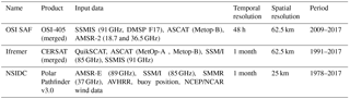
We use the low-resolution sea ice drift data set from the Ocean and Sea Ice Satellite Application Facility (OSI SAF), specifically the OSI-405 multi-sensor product. Various sensors and channels are processed in order to produce the merged product used here: SSMIS (91 GHz H&V polarization) on board DMSP platform F17, ASCAT (C-band backscatter) on board platform Metop-A and AMSR-2 on board JAXA platform GCOM-W. Ice drift is estimated by an advanced cross-correlation method (continuous maximum cross-correlation, MCC) on pairs of satellite images (Lavergne et al., 2010). The merged product considers the different single-sensor data and their quality statistics in order to compensate for data gaps in the single-sensor products. We use this multi-sensor data set, since we require sufficient data coverage in the Fram Strait area, which is not given by the single sensor products. Displacements and geographic coordinates of the start and end points of the displacements for 48 h time spans are provided on a 62.5 km × 62.5 km polar stereographic grid. In the following we refer to this product as OSI SAF.
2.1.2 Ifremer
From the Ifremer-CERSAT (Centre ERS d'Archivage et de Traitement) data set, we use the merged product, which is obtained from combining Advanced Scatterometer (ASCAT) data and special sensor microwave/imager (SSM/I) brightness temperature measurements. It is provided for different time spans, including monthly lags, which is suitable for our study. The algorithm used to deduce ice drift from scatterometer data and the merging with radiometer data is described in Ezraty et al. (2007) and Girard-Ardhuin and Ezraty (2012). Geographic coordinates of the start and end points of the displacements are provided on a 62.5 km × 62.5 km polar stereographic grid. In the following we refer to this product as Ifremer.
2.1.3 NSIDC
Finally, we also use the Polar Pathfinder Sea Ice Motion Vectors data set (version 3), distributed by the National Snow and Ice Data Center (NSIDC). It provides a year-round ice drift data set. As for OSI SAF and Ifremer, ice drift is obtained from multiple satellite sensors, including radiometers and scatterometers (Table 1), complemented by buoy observations from the International Arctic Buoy Program (IABP). During summer, NCEP/NCAR winds speeds are used to estimate ice drift when satellite data are not available. Though we do not make use of the summer ice drift data, we choose to include this data set, since it is widely used in other studies (e.g. Krumpen et al., 2016 and Spreen et al., 2011). Monthly displacements in x and y directions are provided on an EASE 2 25 km × 25 km polar stereographic grid. In the following we refer to this product as NSIDC. In contrast to OSI SAF and Ifremer, NSIDC is only available until February 2017, which means that we do not consider the winter season 2016–2017 for NSIDC.
2.2 AWI CS2 sea ice thickness
We use the AWI CS2 product (processor version 1.2). Processing is based on CS2 orbit data files provided by ESA. Radar waveforms are processed according to Hendricks et al. (2016) and Ricker et al. (2014), using a 50 % threshold first-maximum retracker to obtain ellipsoidal surface elevations (Ricker et al., 2014; Helm et al., 2014). Radar waveforms from surfaces that contain openings in the ice pack appear as specular echoes and can be separated from diffuse echoes that contain reflections from sea ice only. Based on this surface-type classification, open-water elevations are identified and used to derive the instantaneous sea-surface height anomaly by interpolation. To retrieve sea ice freeboard, the sea-surface height anomaly is subtracted from the ice surface elevations.
Freeboard is converted into sea ice thickness by assuming hydrostatic equilibrium (Laxon et al., 2003). For the conversion, we use ice densities of 916.7 and 882.0 kg m−3 for FYI and MYI respectively (Alexandrov et al., 2010), and 1024 kg m−3 for the sea water density. Snow depth and density are deduced from the Warren snow climatology (W99) (Warren et al., 1999). The climatology is modified by reducing the snow depth by 50 % over FYI to take into account the recent change towards a seasonal Arctic ice cover (Kurtz and Farrell, 2011). FYI and MYI are identified with the daily OSI SAF sea-ice-type product (Aaboe et al., 2016). In order to obtain a sufficient spatial coverage, acquired thickness data are averaged monthly on an 25 km EASE 2 grid.
The observational CS2 uncertainties of sea ice thickness contain contributions that are associated with speckle noise, sea-surface height estimation, snow depth and densities of ice and snow (Ricker et al., 2014). They can easily reach values of >1 m for single measurements, but will be reduced to the range of centimetres by spatial averaging. Note that, during the melting period from May to September, the presence of melt ponds prevents the retrieval of sea ice thickness observations.
2.3 OSI SAF ice concentration and type
We use the sea ice concentration (OSI-401) and sea-ice-type product (OSI-403) of the European Organisation for the Exploitation of Meteorological Satellites (EUMETSAT) Ocean and Sea Ice Satellite Application Facility (OSI SAF). Ice concentration is computed from radiometer data using a combination of state-of-the-art algorithms (Tonboe et al., 2017). Ice type is derived from passive microwave and active microwave scatterometer data combined in a Bayesian approach (Aaboe et al., 2016). Ice concentration is needed for the ice volume computation for each 25 km grid cell and ice type is used to classify grid cells as FYI or MYI. The products are updated daily and the data are provided on a 10 km polar stereographic grid. To be consistent with the CS2 product, monthly means are projected onto the EASE2 25 km grid. Ice-type grid cells originally flagged as ambiguous are replaced by an inverse-distance interpolation to obtain FYI or MYI flags for all ice-covered grid cells. Errors can occur due to new ice forming in leads within the MYI zone that are not captured and therefore classified as MYI. Especially in the Fram Strait, where floes can break up into many smaller pieces, this might lead to significant errors in the MYI fraction. Moreover, we have observed erroneous MYI classification in the Arctic Basin during winter 2016–2017. The reason is not yet clear but could be a result of external factors such as exceptionally warm winter temperatures. Therefore, FYI–MYI separation for 2016–2017 should be considered with caution (Signe Aaboe, personal communication, 2017).
2.4 Retrieving ice volume flux and export rates through Fram Strait
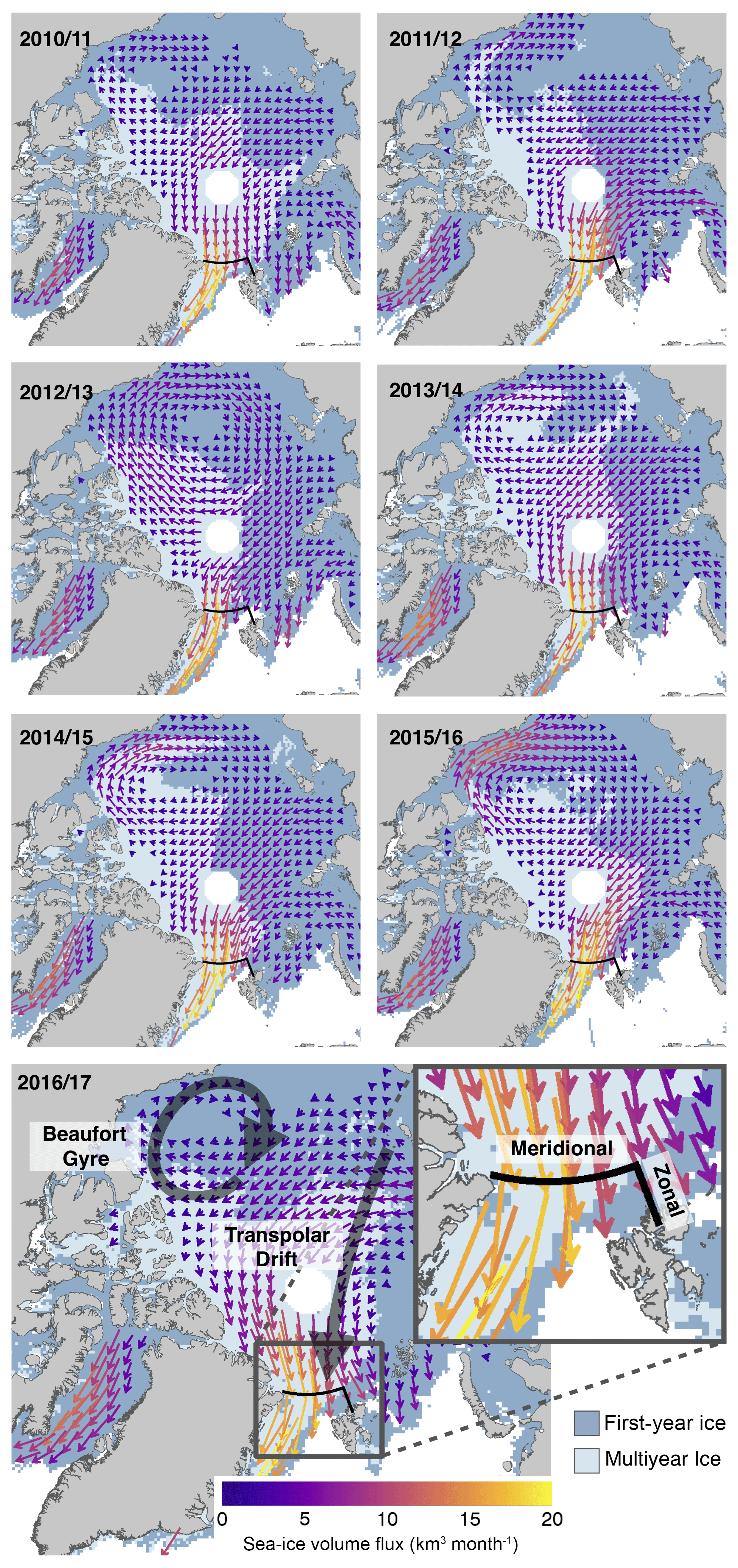
Figure 1Averages of Arctic sea ice volume fluxes for 2010–2011 and 2016–2017 between October and April. The enlarged box shows the location of the Fram Strait gate at 82∘ N, which is used for the calculation of the export rates, separated into meridional and zonal gates.
The first step is to project the ice drift and thickness data onto a common grid. The EASE 2 grid is based on an equal-area projection, and therefore, it is reasonable to use it for sea ice volume estimations (Ricker et al., 2017a). Hence, we define the 25 km EASE 2 grid provided in the AWI CS2 ice thickness product as our standard grid and interpolate the displacement data onto this grid. Since the NSIDC displacement data are already projected on an EASE grid, we only interpolate the displacements in x and y directions onto the 25 km grid. In contrast, the Ifremer and OSI SAF grids are based on a polar stereographic projection. Here, we use the geographic coordinates of the start and end points of the displacement and project them onto the EASE 2 grid separately. Afterwards, displacements in x and y directions of the EASE 2 grid are calculated. Since the Ifremer and NSIDC products are provided as monthly means, the daily updated OSI SAF 48 h displacements need to be summed up to monthly retrievals. Here, we calculate the displacements in x and y directions on the EASE 2 grid for each day and sum them up over 1 month.
Monthly ice volume flux Qx,y in x and y directions is obtained by the following:
where l=25 km is the size of the grid cells, H is the CS2 sea ice thickness, C is the ice concentration obtained from the OSI SAF product, and Dxy represents the ice drift in x and y directions respectively.
In order to compute ice volume export through Fram Strait, we follow the methodology of Krumpen et al. (2016) and define a gate that is a composite of a meridional and a zonal gate (Fig. 1). The meridional gate is located along 82∘ N between 12∘ W and 20∘ E. The zonal part is located along 20∘ E between 80.5 and 82∘ N. We have chosen this gate location to reduce errors and biases in low-resolution ice drift data that become larger with increasing ice velocities, typically found south of 82∘ N (Sumata et al., 2014, 2015). Moreover, uncertainty of CS2 ice thickness increases at lower latitudes, especially near Fram Strait due to sparse orbit coverage (Ricker et al., 2014).
Meridional components Qv of the ice volume flux through the defined gate are calculated as follows:
The zonal components Qu of the ice volume flux are computed accordingly:
where 45∘ W E is the longitude of the respective grid cell and luv the length of the grid cell as a function of λ:
Uncertainties of Qv are estimated by
Zonal uncertainties are calculated accordingly. Consistent with Laxon et al. (2013) and Ricker et al. (2017a), we set the ice concentration uncertainty to %. Nevertheless, we acknowledge that the uncertainty may vary depending on the actual ice concentration (Ivanova et al., 2014). Sea ice thickness uncertainty σH is provided in the AWI CS2 ice thickness product (Ricker et al., 2014). Ice drift uncertainty σD is estimated using the empirical error functions for monthly mean Arctic sea ice drift given in Sumata et al. (2015), which utilizes drift estimates from high-resolution SAR data as a reference:
with the drift error functions ϵx,y in x and y directions of the grid used in Sumata et al. (2015):
where σx,y are standard errors in the x and y directions given in Sumata et al. (2015) for different categories of drift speed and ice concentration for each of the three drift products. Here, we use standard errors for the highest drift speed (>4.3 km d−1). δx,y represents the error of the reference drift data set provided in Sumata et al. (2015). The deduced drift uncertainties for the low-resolution drift products are in the range of 1.0 km d−1, which is comparable to uncertainties estimated in previous studies (Spreen et al., 2009). These estimates do not include systematic errors. A comparison of different drift products in Sumata et al. (2014) shows significant systematic differences between the different drift products, especially for high drift speeds. Since we aim to investigate variabilities in ice volume export, we do not consider potential biases in this study.
We obtain the total ice volume flux through the Fram Strait (QEx) by adding up the meridional zonal grid cell fluxes Qv and Qu along the gate:
Note that, following the axis conventions, ice volume export QEx has a negative algebraic sign, corresponding to a sea ice loss from the Arctic Basin.
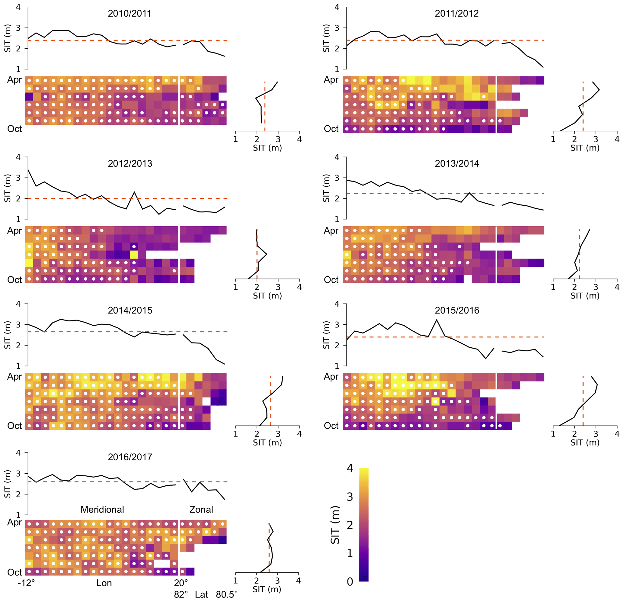
Figure 2Spatio-temporal variability in sea ice thickness (SIT) at the Fram Strait gate from October to April between 2010 and 2017. Upper sub-panels show the temporally averaged SIT. Right sub-panels show the average over the gate SIT for each month within the October–April period. The white dots represent grid cells that contain multi-year ice.
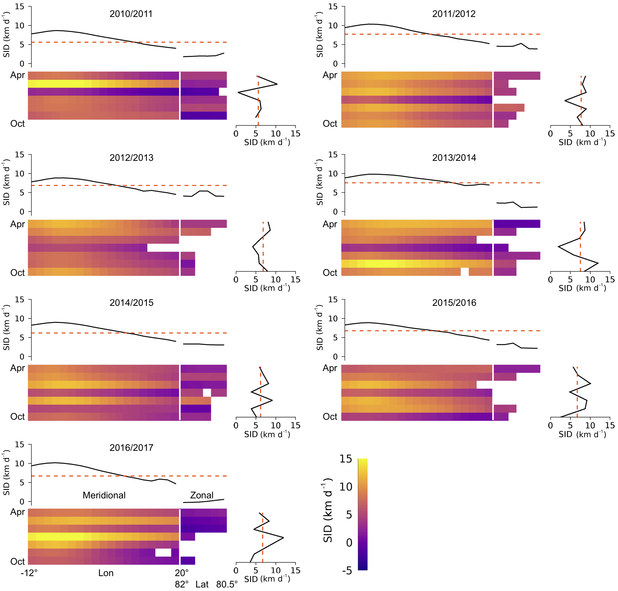
Figure 3Spatio-temporal variability in OSI SAF sea ice drift (SID) at the Fram Strait gate from October to April between 2010 and 2017. Upper sub-panels show the temporally averaged SID. Right sub-panels show the average over the gate SID for each month within the October–April period.
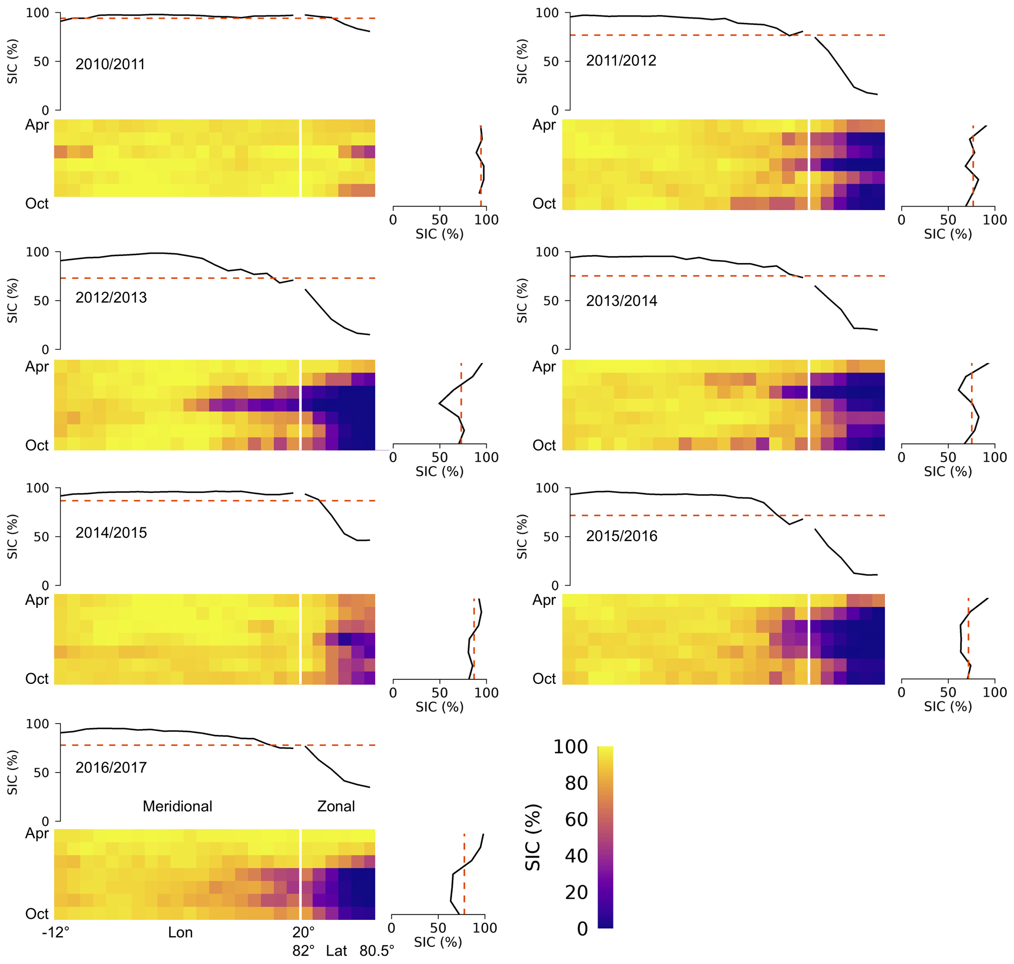
Figure 4Spatio-temporal variability in OSI SAF sea ice concentration (SIC) at the Fram Strait gate from October to April between 2010 and 2017. Upper sub-panels show the temporally averaged SIC. Right sub-panels show the average over the gate SIC for each month within the October–April period.
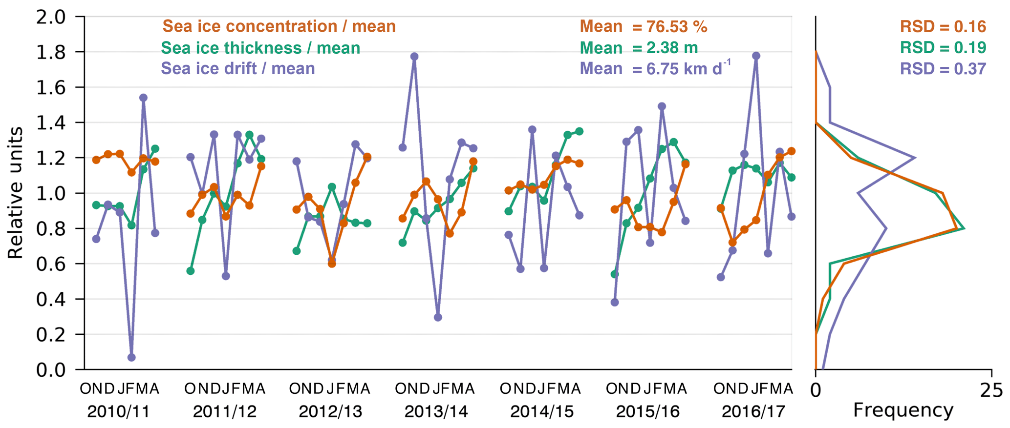
Figure 5OSI SAF sea ice drift, ice thickness and ice concentration averaged over the entire Fram Strait gate, between October and April for winter seasons 2010–2011 to 2016–2017. Monthly values are divided by the mean of the data set for each parameter. The right box shows the corresponding histograms with the relative standard deviations (RSD).
In this section, we first examine sea ice drift, thickness and concentration at the Fram Strait gate. Throughout the study, we use the OSI SAF drift as the reference product, because it shows the best performance among the used products in the Fram Strait (Sumata et al., 2014). Second, we present estimates of the ice volume flux in the Arctic and the calculated export through Fram Strait. Third, we examine the choice of the drift product, computing ice volume export using also Ifremer and NSIDC ice drift estimates. Throughout the paper, we refer to the winter period from October to April (OA). However, seasonal export estimates are calculated by adding together the monthly export from November to April (NA), since we have no ice thickness estimates for October 2010.
3.1 Sea ice drift, thickness and concentration at the gate
We consider all input parameters for Eq. (1), sea ice thickness (H), sea ice drift (D) and ice concentration (C). Figure 2 shows the spatio-temporal distribution of CS2 ice thickness along the meridional and zonal gates through each winter season, separated into FYI and MYI. Ice thickness along the gate is variable and ranges from 0 to 5 m. The mean gate thickness reveals a consistent gradient from thinner ice in October to thicker ice in April in all years, although the gradient can be small for some years (e.g. 2016–2017). Averaging over each OA period reveals the spatial thickness distribution along the meridional and zonal gates. In 2012–2013 and 2013–2014, we find a significant positive thickness gradient towards the coast of Greenland, while in other years, this is less pronounced. At the zonal gate, ice thickness decreases towards Svalbard. During winter seasons 2011–2012, 2012–2013 and 2013–2014, the fraction of grid cells that contain MYI is lower compared to other years. In 2012–2013 and 2013–2014, the lack of MYI in the eastern part of the gate is replenished by FYI that is thinner than 1.5 m. In seasons 2010–2011 and 2016–2017, the MYI fraction at the zonal gate is larger than in other years. In 2011–2012, from February to March, the indicated FYI is rather thick (>2 m), similarly to the indicated MYI towards the coast of Greenland.
Figure 3 shows the spatio-temporal distribution of the OSI SAF ice drift along the meridional and zonal gates through each winter season. In contrast to ice thickness, the drift reveals a larger temporal variability with monthly differences of up to 10 km d−1 and without a distinct trend within each winter season. On the other hand, the OA period averages of the drift show a consistent spatial trend for all years, from less than 5 km d−1 in the east (20∘ E) and at the zonal gate, to a maximum of 9–10 km d−1 at about 6∘ W, followed by a decrease towards the coast of Greenland. The stationary peak at about 6∘ W suggests a large-scale forcing and could be associated with the East Greenland Current (Rudels et al., 2002; de Steur et al., 2009). We notice that mean drift across the zonal gate is only 35 % of the mean drift across the meridional gate. The Ifremer and NSIDC ice drift also exhibit similar patterns to OSI SAF (not shown).
Figure 4 shows the spatio-temporal distribution of the ice concentration along the meridional and zonal gates through each winter season. Ice concentration at the meridional gate is persistently high and ranges between 70 % and 100 %, with a few exceptions like January 2012–2013. In contrast, the zonal ice concentration shows higher variability, depending on the ice extent north of Svalbard, where the ocean remains ice-free in some areas over several months.
Figure 5 illustrates ice drift, thickness and concentration averaged over the entire gate and divided by their mean values to illustrate their variability and make it comparable. Here, ice concentration represents the fraction of ice covered area along the entire gate, including the zonal and meridional parts. As indicated in Fig. 2, in contrast to ice drift, ice thickness shows a trend in most of the winter seasons. The same holds for the ice concentration as ice extent at the zonal gate north of Svalbard increases during winter in most of the seasons (Fig. 4). In 2010–2011, the gate was almost entirely ice covered during the OA period. The histograms refer to the drift, thickness and concentration time series over the entire 7-year period. The drift distribution reveals two modes and a larger degree of dispersion than the ice thickness and concentration distribution. In order to compare and quantify the extent of variability in the three parameters we compute their relative standard deviation (RSD), which is the ratio of the standard deviation to the mean. We find that the RSD of the ice drift (0.37) is roughly double the RSD of ice thickness (0.19) and ice concentration (0.16).
3.2 Sea ice volume flux and export through the Fram Strait
Figure 1 shows the retrieved ice volume flux as means over the OA period for the Northern Hemisphere for the 7 years of the CS2 operational period (2010–2017), using OSI SAF ice drift data. The two major patterns are the Beaufort Gyre and the Transpolar Drift conveying ice towards Fram Strait. There, the ice fluxes reach maximum values of 20 km3 month−1 or more, with a steep gradient along a north–south axis. The maximum values have to be considered in relation to the 25 km grid resolution. MYI is mainly exported through the meridional part of the gate, while sea ice at the zonal part is primarily FYI. The monthly sea ice volume export through Fram Strait is shown in Table 2 and Fig. 6. During the 7-year period, the maximum monthly ice volume export of −540 km3 month−1 occurs in March 2011, while the minimum of −21 km3 month−1 is found in February 2011. Table 3 provides the total ice volume export (QEx,OSISAF) through the Fram Strait gate for the NA period. We find a maximum export of km3 for 2011–2012 and a minimum of km3 in 2012–2013. The major fraction of exported sea ice is represented by MYI. However, in a few months like April 2012, the fraction of exported FYI exceeds the MYI fraction. Table 3 shows the fraction of exported MYI averaged over the seasons. A maximum of 94 % occurs in 2016–2017 and a minimum of 64 % occurs in 2012–2013. The MYI fraction refers to grid cells which are indicated as MYI by using the ice-type product.
3.3 Deriving sea ice volume export using different ice drift products
In order to investigate the impact of the chosen drift product on the volume export estimates, we compare ice volume flux through the Fram Strait gate using three different drift products. Figure 7a shows an example for monthly ice volume flux through the Fram Strait gate and the contributions to the meridional and zonal parts of the gate, using the three drift products. All three retrievals exhibit consistent temporal and spatial variations along the gate but differ in magnitude. QEx,OSISAF and QEx,Ifremer always exceed QEx,NSIDC by about 0.2–0.3 km3 day−1. Uncertainties of the ice flux through each grid cell are in the range of 0.1 km3 day−1. Figure 7b shows the monthly and seasonal ice volume export through the Fram Strait during the NA period between 2010 and 2017, computed with the three different drift products. The variations of QEx,OSISAF and QEx,Ifremer correlate, but differ in magnitude. Table 3 provides the corresponding annual differences between the products. Using Ifremer ice drift, the derived ice export is 200–500 km3 lower than export derived using OSI SAF ice drift, which corresponds to a mean difference of about −23 %. QEx,NSIDC is the lowest among the three estimates and shows mean difference of about −26 %, relating to QEx,OSISAF. Also, the interannual changes of QEx,NSIDC compared to both QEx,OSISAF and QEx,Ifremer are slightly different as QEx,NSIDC decreases from 2010–2011 to 2011–2012, while the other retrievals show an increase. In 2011–2012, the monthly difference of QEx,NSIDC from the other retrievals is significantly higher than in other winter seasons, but the reason for this is unclear. Nevertheless, the main variations and the magnitudes of spatial gradients are similar for all products. Considering the correlation coefficients (r) between the monthly volume export retrievals (Fig. 7b, upper panel), we find r(QEx,OSISAF, , and . Therefore, the choice of the drift products has no major impact on our export variability analysis. We also note that it is not within the scope of this work to determine which product provides the most accurate estimate of sea ice drift in the Fram Strait.
Table 2Monthly Arctic sea ice volume export through the Fram Strait in km3 month−1 computed with OSI SAF ice drift. Maximum and minimum values are denoted in italic and bold, respectively.
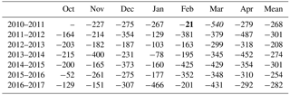
Table 3Total Arctic sea ice volume export through the Fram Strait for winter seasons 2010–2011 and 2016–2017, added together over the November–April period. Volume export has been computed using three different ice drift products, using QEx,OSISAF as the reference product. The last column shows the fraction of exported multi-year sea ice (% MYI).
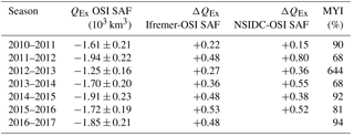
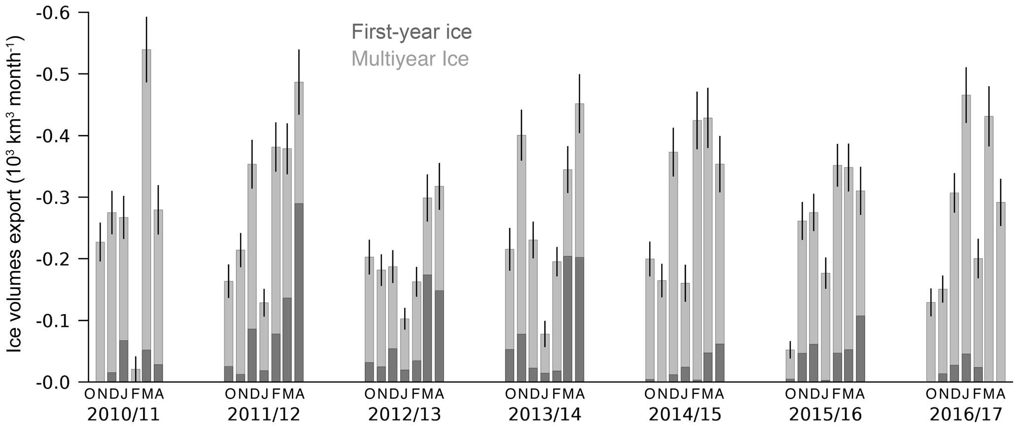
Figure 6Monthly sea ice volume export through Fram Strait from October to April for the period 2010–2011 and 2016–2017, using the OSI SAF ice drift product. The volume export is divided into first- and multi-year sea ice. Uncertainties are represented by error bars. October 2010 data are missing due to the unavailability of CryoSat-2 data.

Figure 7(a) Example for monthly ice volume export through the Fram Strait gate (April 2012) derived from three different ice drift products. (b) Monthly sea ice volume export (upper panel) and total Arctic sea ice volume export through the Fram Strait for winter seasons 2010–2011 and 2016–2017, added together over the November–April period and derived from three different ice drift products (lower panel). Mean Arctic Oscillation (AO) Index and mean North Atlantic Oscillation Index (NAO) are shown for the same period, including coefficients of determination (r2).
4.1 Relative contribution of sea ice drift, thickness and concentration to the volume flux variability
In order to understand the mechanisms behind the variability in ice volume export, we now examine the three input parameters, ice drift, thickness and concentration, in more detail. As shown in Sect. 3.1, the thickness averaged across Fram Strait exhibits significant interannual changes, with an overall increase in spring. This increase at the gate from autumn to spring can be associated with the thermodynamic ice growth and deformation of FYI and thin second-year ice. For example, in 2011–2012 and 2013–2014, thickness of FYI grid cells rises from October to April (Fig. 2). In contrast, in 2016–2017, the fraction of FYI passing the gate is only 6 %, and consequently, we do not observe significant changes in mean ice thickness during the OA period. Similarly, we observe an increase in mean ice concentration at the gate during the OA period. Considering the ice drift, we find opposite features. The mean monthly drift in the time domain is highly variable, without a distinct trend over the OA period (Fig. 8a). These characteristics of the variability in input parameters affect the mean monthly ice volume export (Fig. 8b). The mean seasonal cycle over the period 2010–2017 is characterized by minima in October and January and the maximum in March. Considering seasonal cycles of drift, thickness and concentration at the gate and comparing them with the seasonal cycle of the ice export, we find that the variability is mostly explained by the ice drift (Fig. 8a) as also suggested by the RSD. On the other hand, the positive gradient of the ice volume export between autumn and spring with the annual maximum in March can be associated with the seasonal cycle of sea ice thickness (Fig. 8a). This seems primarily driven by thermodynamic ice growth and deformation. Although the seasonal cycle of mean ice concentration along the entire gate shows positive gradients as well, with a similar RSD to the ice thickness, it seems to play a minor role for the ice export variability. This is because ice concentration variability at the meridional gate is small due to the persistent ice coverage over the season. Considered separately, we find a RSD of 0.78 at the zonal gate and a RSD of 0.08 at the meridional gate. However, due to the smaller size, lower ice drift and thinner ice, the zonal volume flux is only about 4 % of the total ice export over the 7-year period.
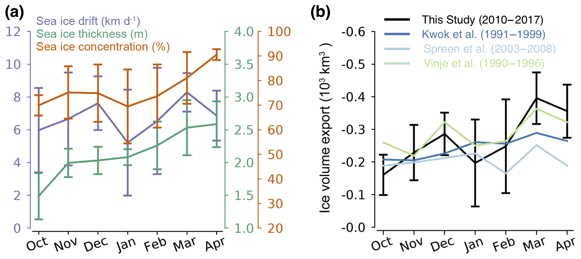
Figure 8(a) Mean monthly sea ice drift, thickness and concentration at the Fram Strait gate over the years 2010–2011 and 2016–2017 with corresponding standard deviations. (b) Mean monthly ice volume export through the Fram Strait from this study and from Spreen et al. (2009), Kwok et al. (2004) and Vinje et al. (1998), covering different periods.
4.2 Comparison to previous studies
Sea ice export through the Fram Strait and its variability have been the focus of several previous studies. A major difference in the method is the choice of the position of the gate. Smedsrud et al. (2017) placed the gate at 79∘ N, Spreen et al. (2009) placed their northernmost gate at 80∘ N, and Kwok and Rothrock (1999) placed their gate at about 81∘ N. Except for the study of Krumpen et al. (2016), all these studies use only a meridional gate or a straight connection between Greenland and Spitsbergen. The major advantage of using a gate positioned further north, like at 82∘ N, is that ice motion products and thickness estimates from satellites show lower uncertainties at this latitude. Indeed, errors and biases of low-resolution ice drift data derived from passive microwave and scatterometer data become larger as ice velocity increases, and velocity tends to be larger with steeper gradients south of 82∘ N (Sumata et al., 2014, 2015). In addition, uncertainty of CS2 ice thickness increases at lower latitudes, especially in Fram Strait due to sparse orbit coverage (Ricker et al., 2014, 2017b). Therefore, we followed the approach of Krumpen et al. (2016), placing the gate at 82∘ N, which appears to be a good choice for reducing uncertainty associated with our ice volume export estimate.
Figure 8b shows the mean monthly winter export from October to April from this study compared to previous estimates (Kwok et al., 2004; Spreen et al., 2009; Vinje et al., 1998). Vinje et al. (1998) and Kwok et al. (2004) use ULS data for the estimation of ice thickness in the Fram Strait. Vinje et al. (1998) use ULS ice draft measurements from 1990 to 1996 in combination with buoy and SAR-based ice drift estimates, and estimate ice volume fluxes through the Fram Strait that show maxima of up to about −600 km3 month−1. Kwok et al. (2004) investigated nearly the same period (1991–1999) and find a maximum monthly export of −509 km3 month−1 in December 1994. Their estimates are generally lower than in Vinje et al. (1998). Spreen et al. (2009) use ice thickness and drift estimates derived from satellite data to compute ice volume flux, and therefore, their study is methodically similar to our work. However, besides the gate at 80∘ N, they use a different ice thickness retrieval (ICESat) and another low-resolution ice drift data set (Cersat/Ifremer, AMSR-E) to derive ice volume export. For the period 2003–2008, they estimate monthly winter ice volume export ranging from −100 to −420 km3 month−1, using ULS ice thickness estimates to complement the 2-month-long ICESat measurement periods per year. The largest difference of about 150 km3 between the lowest and largest estimate is found in March. Our estimate seems to be the one with the highest change between October and April; e.g. our estimates are lowest in October and highest in April (Fig. 8b). Our seasonal cycle also reveals higher variability. Several factors might cause this discrepancy:
-
The observing periods are not overlapping, and therefore, differences in mean monthly export can be caused by natural variations in ice thickness and drift.
-
Bottom melt due to the recirculation of warm Atlantic water between 82 and 80∘ N might lead to a reduction in ice volume (Wekerle et al., 2017).
-
The low resolution of the drift data might lead to systematic uncertainties in the volume flux at the gate, especially near the coast and the ice margins, affecting all retrievals.
-
Systematic differences between the CS2 and ICESat ice thickness retrievals may appear because of different retrieval algorithms and different sensor characteristics.
-
Ice drift at 80∘ N might be underestimated due to large ice velocities, which are not well captured in radiometer- and scatterometer-based drift products.
Despite these differences, estimates from different studies exhibit consistent features, such as the maximum in March. In the following, we will discuss the interannual variability and the role of atmospheric circulation patterns.
4.3 Interannual ice volume export variability
The time series of winter ice volume export through the Fram Strait reveals a significant decrease of 500 km3 from 2011–2012 to 2012–2013 (Fig. 7). This decrease is characterized by a drop in both the mean ice drift and the thickness through Fram Strait. Comparing the pan-Arctic ice condition in both winters, a decrease in ice thickness north of Fram Strait has been reported for 2012–2013 by Ricker et al. (2017a) and was found to be mainly a result of anomalous summer melt and late freeze-up in 2012. The ice in the area north of Fram Strait is the main source of exported ice (Smedsrud et al., 2017), and thus we also find a drop in ice thickness at the Fram Strait for 2012–2013, which is accompanied by a lower mean drift (Fig. 5). In contrast, in winter season 2013–2014, which followed a cold Arctic summer with low melt rates (Tilling et al., 2015), ice thickness at the gate increased, accompanied by a higher mean drift (Fig. 5). This results in an ice volume export comparable to 2010–2011 (Fig. 7).
We also examine the link between ice volume export and North Atlantic Oscillation (NAO) index and the Arctic Oscillation (AO) index (Fig. 7b). The NAO index is defined as the sea level pressure anomaly between Lisbon, Portugal, and Reykjavik, Iceland. A positive NAO index is associated with an Icelandic low and a corresponding high-pressure system over the Azores. When the Icelandic low is intensified, the sea level pressure gradient in the Fram Strait increases, leading to strong northerly winds and hence increased sea ice drift (Kwok and Rothrock, 1999; Kwok et al., 2013; Ionita et al., 2016; Smedsrud et al., 2017). Thus, a high, positive NAO index is associated with high ice volume export rates, since ice drift primarily drives the ice volume export variability. If both pressure systems are weak or even reversed, the NAO phase becomes negative and correlation between NAO and sea level pressure gradient along the Fram Strait decreases. The variability in the NAO is largest during the winter season. We have obtained monthly NAO indices from the National Oceanic and Atmospheric Administration (NOAA) and averaged them over the NA period. Positive phases (>1) of the NAO index occurred in 2011–2012 and 2014–2015, coinciding with increased mean monthly ice volume export rates (Fig. 7b).
The sea level pressure gradient variability through the Fram Strait is also captured in the AO and its corresponding index, described in Thompson and Wallace (1998). The AO pattern involves an oscillation of the sea level pressure between the Arctic basin and the surrounding zonal belt. The AO therefore includes characteristics of the NAO, which is regionally bounded. We have obtained monthly AO indices from NOAA (http://www.cpc.ncep.noaa.gov, last access: 18 September 2018) and averaged them over the NA period. The variability in the AO index is similar to the variability in the NAO index and the ice volume export, especially if the flux is computed with Ifremer and OSI SAF ice drift (Fig. 7b). The correlation between ice export and AO index (r2=0.87) is larger than with the NAO index (r2=0.74). This is because the NAO index decreases in 2016–2017, while the ice volume export increases compared to the previous year. However, we acknowledge that a longer time series is required to obtain statistical meaningful correlation coefficients.
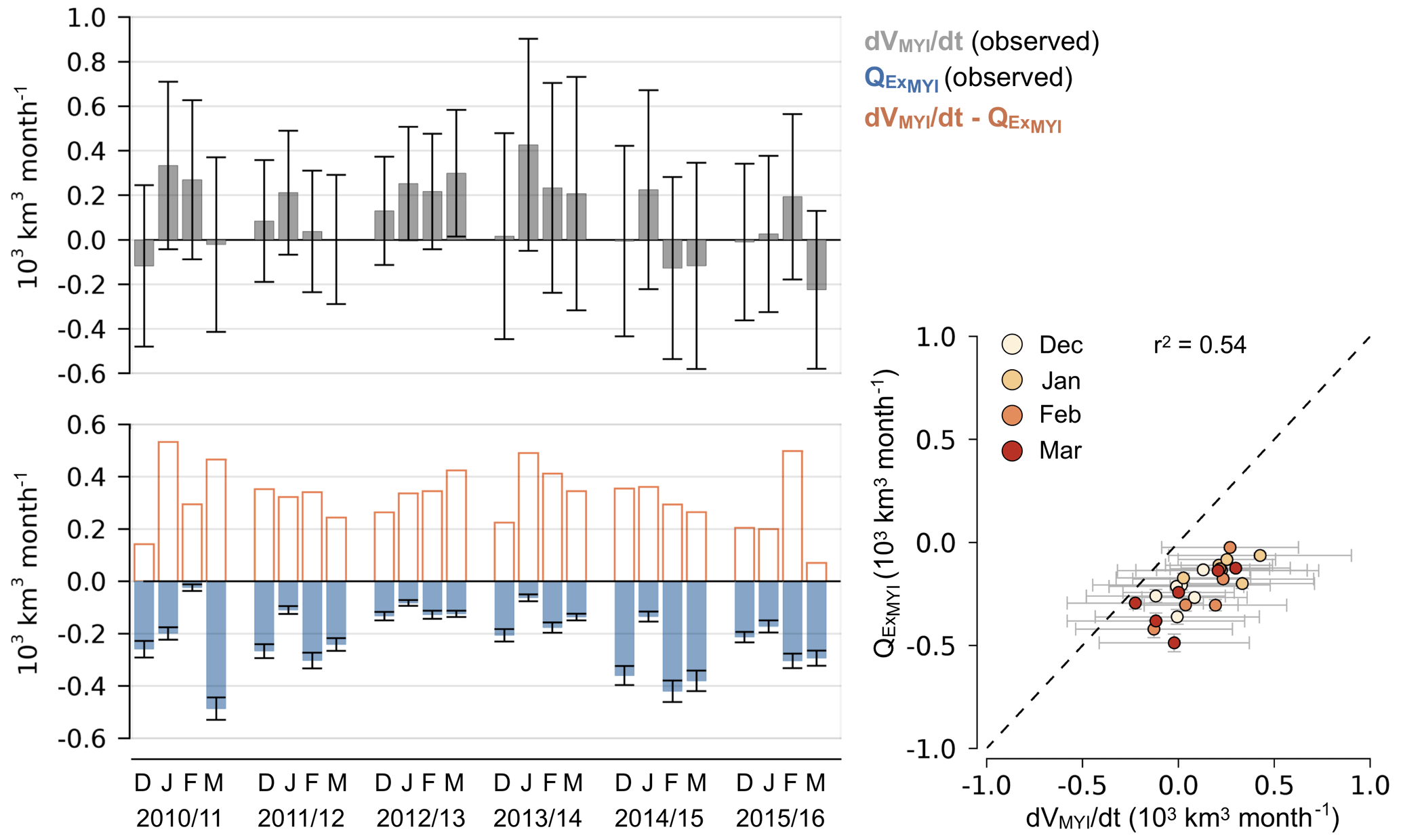
Figure 9Monthly MYI volume export through the Fram Strait () and simultaneous Arctic MYI volume growth rates (dVMYI∕dt) between December and March for the winter seasons 2010–2011 and 2015–2016. Error bars represent the corresponding uncertainties. The scattergram shows the relation between dVMYI∕dt and , and the corresponding coefficient of determination (r2).
4.4 The impact of ice volume export on Arctic ice mass balance
Kwok et al. (1999) investigated the area balance of the Arctic Ocean perennial ice zone between October 1996 and April 1997. Using RADARSAT data, they reported that winter MYI area loss can be explained almost entirely by ice export. Moreover, their findings suggest that export is dominated by ice flux through the Fram Strait, while export through other gates like Nares Strait plays a minor role. According to Kwok et al. (1999), MYI area export through Nares Strait is about 5 % of the Fram Strait MYI area export. The balance of the MYI area is only affected by export and ice dynamics, assuming that the net melt of the MYI area is zero in winter. As a consequence, the Arctic MYI area decreases from October to April, and in turn, this decrease is almost entirely balanced by exported MYI area (Kwok et al., 1999).
In the following, we investigate the ice volume balance of the Arctic MYI. In contrast to the MYI area, we assume that MYI volume growth rate of the Arctic Ocean domain (dVMYI∕dt) is affected by both export () and ice volume gain due to thermodynamic growth (). Neglecting net melt of MYI in winter, we can write the following:
The term accounts for residual contributions. This includes ice deformation that might change the bulk ice density, which we assume to be constant. Moreover, newly formed openings within the MYI zone due to divergence can bias the ice-type classification when such areas are erroneously classified as MYI. This effect leads to a positive bias of dVMYI∕dt. A quantitative separation between and is difficult. Therefore, we only consider the entire contribution of the second term in Eq. (9).
We estimate monthly Arctic MYI volume growth dVMYI∕dt by a 3-point Lagrangian interpolation scheme, where we exclude all ice south of the Fram Strait gate. Since CS2 ice thickness data are not available in October 2010, we compute dVMYI∕dt using data over the NA period and therefore obtain dVMYI∕dt values for December to March. Figure 9 shows monthly dVMYI∕dt and corresponding for 6 years. In addition, it shows the residual ( + ), which is not directly observed, but deduced by subtracting from dVMYI∕dt. Winter season 2016–2017 is excluded here due to erroneous MYI ice classification, which affects dVMYI∕dt and (Sect. 2.3).
MYI volume growth dVMYI∕dt does not follow a seasonal cycle as it is the case for FYI volume growth that is primarily driven by the thermodynamic ice growth (Ricker et al., 2017a). It appears that is just in the range to almost or entirely balance the volume gain of the second term in Eq. (9), (). For example, in 2014–2015 and 2015–2016, mean dVMYI∕dt is nearly zero due to large between December and March. It is possible that exceeds , leading to a net reduction in Arctic MYI volume when considering a positive bias due to erroneous MYI-type classification. However, the variability of dVMYI∕dt is significantly driven by , revealing a coefficient of determination (r2) of 0.54, which means that 54 % of dVMYI∕dt during winter can be explained by variations of , assuming a linear relationship. From that, we can deduce that the variability of dVMYI∕dt is significantly driven by the variability in the ice drift in the Fram Strait.
The high correlation (0.74) between and dVMYI∕dt is also noticeable. This proves the accuracy of Arctic MYI volume estimates, as the correlation between and dVMYI∕dt exposes the signal of ice volume export in the MYI volume budget. In the case of large errors in dVMYI∕dt as indicated in Fig. 9 by the error bars, correlation with would be degraded.
Here we have used, for the first time, the CryoSat-2 ice thickness retrievals in order to quantify the sea ice export through Fram Strait. We performed a detailed analysis of variability and important processes for the Arctic multi-year ice (MYI) mass balance. Based on our analysis, the following conclusions can be drawn:
-
Based on different ice drift products, the three ice volume export retrievals (QEx,OSISAF, QEx,Ifremer, QEx,NSIDC) exhibit similarities in their variability (correlations r>0.9), although they differ in magnitude by −23 % (QEx,Ifremer) and −26 % (QEx,NSIDC), compared to QEx,OSISAF. In order to investigate long-term trends in ice volume export derived from multiple satellite observations, we therefore need to construct multi-sensor consistent time series of ice drift, thickness and concentration. Moreover, a consistent methodology to compute ice volume flux through Fram Strait is required.
-
Ice drift shows coherent spatial variability across Fram Strait, but high-frequency variability from month to month. The mean monthly ice drift across Fram Strait shows a peak at about 6∘ W, which could be associated with the East Greenland Current.
-
The relative standard deviation (RSD) is a measure that compares the variability of different physical quantities. At the Fram Strait gate, RSD of ice drift (0.37) is roughly twice as high as the RSD of ice thickness (0.19) and concentration (0.16) for the observation periods of 2010–2011 and 2016–2017, revealing that ice drift is the main driver of seasonal and interannual variability of ice volume export. However, the seasonal trend of ice volume export is driven by variations in ice thickness due to the thermodynamic growth that typically leads to a maximum in March. Ice concentration variability is large at the zonal gate (RSD =0.78), but small at the meridional gate (RSD =0.08), where 96 % of the sea ice is exported.
-
Monthly sea ice volume export through Fram Strait varies between −21 and −540 km3 month−1.
-
The interannual variations in ice volume export can be explained by large-scale variability of the atmospheric circulation captured by the Arctic Oscillation (r2=0.87) and North Atlantic Oscillation indices (r2=0.74).
-
While the seasonal cycle of Arctic first-year ice volume is driven by thermodynamic ice growth, 54 % of the changes in Arctic MYI volume over the December–March period can be explained by ice volume export through the Fram Strait.
Sea ice concentration, sea-ice-type and sea ice drift data are provided by OSI SAF (http://osisaf.met.no, EUMETSAT, 2010–2017a, b, c). CryoSat-2 ice thickness data from 2010 to 2017 are provided by http://www.meereisportal.de (Alfred Wegener Institute, 2010–2017). Ifremer ice drift data from 2010 to 2017 are provided via CERSAT (http://cersat.ifremer.fr, CERSAT, 2010–2017). NSIDC ice drift data from 2010 to 2017 are provided via https://nsidc.org (National Snow and Ice Data Center, 2010–2017).
RR conducted the ice volume flux calculations and the analysis. FGA, TK and CL contributed to the analysis of the ice volume flux data. RR wrote the paper and all co-authors contributed to the discussion and gave input for writing.
The authors declare that they have no conflict of interest.
This work has been conducted in the framework of the project: Space-borne
observations for detecting and forecasting sea ice cover extremes (SPICES)
funded by the European Union (H2020) (grant 640161). CryoSat-2 data are
provided by http://www.meereisportal.de (last access: 18 September 2018) (grant REKLIM-2013-04). Moreover, this work was supported by
the German Ministry for Science and Education under grant 03F0777A (QUARCCS)
and the CORESAT project funded by the Norwegian Research Council (grant
222681).
The article processing charges for this open-access
publication were covered by a Research
Centre of the Helmholtz Association.
Edited by: Daniel Feltham
Reviewed by: two anonymous referees
Aaboe, S., Breivik, L.-A., Sørensen, A., Eastwood, S., and Lavergne, T.: Global sea ice edge and type product user's manual, OSI-403-c & EUMETSAT, 2016. a, b
Alexandrov, V., Sandven, S., Wahlin, J., and Johannessen, O. M.: The relation between sea ice thickness and freeboard in the Arctic, The Cryosphere, 4, 373–380, https://doi.org/10.5194/tc-4-373-2010, 2010. a
Alfred Wegener Institute: Helmholtz Centre for Polar and Marine Research, CryoSat-2 Sea Ice Thickness Data Product (v1.2), available at: http://data.seaiceportal.de (last access date: 18 September 2018), 2010–2017. a
Comiso, J. C.: Arctic multiyear ice classification and summer ice cover using passive microwave satellite data, J. Geophys. Res.-Oceans, 95, 13411–13422, https://doi.org/10.1029/JC095iC08p13411, 1990. a
de Steur, L., Hansen, E., Gerdes, R., Karcher, M., Fahrbach, E., and Holfort, J.: Freshwater fluxes in the East Greenland Current: A decade of observations, Geophys. Res. Lett., 36, L23611, https://doi.org/10.1029/2009GL041278, a
Dickson, R. R., Meincke, J., Malmberg, S.-A., and Lee, A. J.: The “great salinity anomaly” in the Northern North Atlantic 1968–1982, Prog. Oceanogr., 20, 103–151, https://doi.org/10.1016/0079-6611(88)90049-3, 1988. a
EUMETSAT: Ocean and Sea Ice Satellite Application Facility, sea ice type product, available at: ftp://osisaf.met.no/archive/ice/type (last access: 18 September 2018), 2010–2017a. a
EUMETSAT: Ocean and Sea Ice Satellite Application Facility, sea ice concentration product, available at: ftp://osisaf.met.no/archive/ice/conc, (last access: 18 September 2018), 2010–2017b.
EUMETSAT: Ocean and Sea Ice Satellite Application Facility, low resolution sea ice drift product, available at: ftp://osisaf.met.no/archive/ice/drift_lr (last access: 18 September 2018), 2010–2017c.
Ezraty, R., Girard-Ardhuin, F., and Piollé, J.-F.: Sea ice drift in the central Arctic estimated from SeaWinds/QuikSCAT backscatter maps, User's Manual, Laboratoire d'Océanographie Spatiale (Département d'Océanographie Physique et Spatiale), IFREMER, Brest, 2007. a
Girard-Ardhuin, F. and Ezraty, R.: Enhanced Arctic Sea Ice Drift Estimation Merging Radiometer and Scatterometer Data, IEEE T. Geosci. Remote, 50, 2639–2648, https://doi.org/10.1109/TGRS.2012.2184124, 2012. a
Helm, V., Humbert, A., and Miller, H.: Elevation and elevation change of Greenland and Antarctica derived from CryoSat-2, The Cryosphere, 8, 1539–1559, https://doi.org/10.5194/tc-8-1539-2014, 2014. a
Hendricks, S., Ricker, R., and Helm, V.: User Guide – AWI CryoSat-2 Sea Ice Thickness Data Product (v1.2), hdl:10013/epic.48201, 2016. a
Holland, M. M., Bitz, C. M., and Tremblay, B.: Future abrupt reductions in the summer Arctic sea ice, Geophys. Res. Lett., 33, L23503, https://doi.org/10.1029/2006GL028024, 2006. a
Ifremer (CERSAT): sea ice drift product, available at: ftp://ftp.ifremer.fr/ifremer/cersat/products/gridded/psi-drift/ (last access: 18 September 2018), 2010–2017. a
Ionita, M., Scholz, P., Lohmann, G., Dima, M., and Prange, M.: Linkages between atmospheric blocking, sea ice export through Fram Strait and the Atlantic Meridional Overturning Circulation, Sci. Rep.-UK, 6, 32881, https://doi.org/10.1038/srep32881, 2016. a, b
Ivanova, N., Johannessen, O. M., Pedersen, L. T., and Tonboe, R. T.: Retrieval of Arctic Sea Ice Parameters by Satellite Passive Microwave Sensors: A Comparison of Eleven Sea Ice Concentration Algorithms, IEEE T. Geosci. Remote, 52, 7233–7246, https://doi.org/10.1109/TGRS.2014.2310136, 2014. a
Krumpen, T., Gerdes, R., Haas, C., Hendricks, S., Herber, A., Selyuzhenok, V., Smedsrud, L., and Spreen, G.: Recent summer sea ice thickness surveys in Fram Strait and associated ice volume fluxes, The Cryosphere, 10, 523–534, https://doi.org/10.5194/tc-10-523-2016, 2016. a, b, c, d, e
Kurtz, N. T. and Farrell, S. L.: Large-scale surveys of snow depth on Arctic sea ice from Operation IceBridge, Geophys. Res. Lett., 38, L20505, https://doi.org/10.1029/2011GL049216, 2011. a
Kwok, R.: Near zero replenishment of the Arctic multiyear sea ice cover at the end of 2005 summer, Geophys. Res. Lett., 34, L05501, https://doi.org/10.1029/2006GL028737, 2007. a
Kwok, R. and Cunningham, G.: Variability of Arctic sea ice thickness and volume from CryoSat-2, Philos. T. R. Soc. A, 373, 20140157, https://doi.org/10.1098/rsta.2014.0157, 2015. a
Kwok, R. and Rothrock, D. A.: Variability of Fram Strait ice flux and North Atlantic Oscillation, J. Geophys. Res.-Oceans, 104, 5177–5189, https://doi.org/10.1029/1998JC900103, 1999. a, b, c
Kwok, R., Cunningham, G. F., and Yueh, S.: Area balance of the Arctic Ocean perennial ice zone: October 1996 to April 1997, J. Geophys. Res.-Oceans, 104, 25747–25759, https://doi.org/10.1029/1999JC900234, 1999. a, b, c, d
Kwok, R., Cunningham, G. F., and Pang, S. S.: Fram Strait sea ice outflow, J. Geophys. Res.-Oceans, 109, c01009, https://doi.org/10.1029/2003JC001785, 2004. a, b, c, d
Kwok, R., Spreen, G., and Pang, S.: Arctic sea ice circulation and drift speed: Decadal trends and ocean currents, J. Geophys. Res.-Oceans, 118, 2408–2425, https://doi.org/10.1002/jgrc.20191, 2013. a
Lavergne, T., Eastwood, S., Teffah, Z., Schyberg, H., and Breivik, L.-A.: Sea ice motion from low-resolution satellite sensors: An alternative method and its validation in the Arctic, J. Geophys. Res.-Oceans, 115, c10032, https://doi.org/10.1029/2009JC005958, 2010. a
Laxon, S., Peacock, N., and Smith, D.: High interannual variability of sea ice thickness in the Arctic region, Nature, 425, 947–950, 2003. a
Laxon, S. W., Giles, K. A., Ridout, A. L., Wingham, D. J., Willatt, R., Cullen, R., Kwok, R., Schweiger, A., Zhang, J., Haas, C., Hendricks, S., Krishfield, R., Kurtz, N., Farrell, S., and Davidson, M.: CryoSat-2 estimates of Arctic sea ice thickness and volume, Geophys. Res. Lett., 40, 732–737, https://doi.org/10.1002/grl.50193, 2013. a
Lique, C., Treguier, A. M., Scheinert, M., and Penduff, T.: A model-based study of ice and freshwater transport variability along both sides of Greenland, Clim. Dynam., 33, 685–705, https://doi.org/10.1007/s00382-008-0510-7, 2009. a
Maslanik, J., Stroeve, J., Fowler, C., and Emery, W.: Distribution and trends in Arctic sea ice age through spring 2011, Geophys. Res. Lett., 38, L13502, https://doi.org/10.1029/2011GL047735, 2011. a
National Snow and Ice Data Center: Polar Pathfinder Daily 25 km EASE-Grid Sea Ice Motion Vectors, Version 3, available at: https://nsidc.org/data/nsidc-0116/versions/3 (last access: 18 September 2018), https://doi.org/10.5067/O57VAIT2AYYY, 2010–2017. a
Parkinson, C. L. and Comiso, J. C.: On the 2012 record low Arctic sea ice cover: Combined impact of preconditioning and an August storm, Geophys. Res. Lett., 40, 1356–1361, https://doi.org/10.1002/grl.50349, 2013. a
Ricker, R., Hendricks, S., Helm, V., Skourup, H., and Davidson, M.: Sensitivity of CryoSat-2 Arctic sea-ice freeboard and thickness on radar-waveform interpretation, The Cryosphere, 8, 1607–1622, https://doi.org/10.5194/tc-8-1607-2014, 2014. a, b, c, d, e, f, g, h
Ricker, R., Hendricks, S., Girard-Ardhuin, F., Kaleschke, L., Lique, C., Tian-Kunze, X., Nicolaus, M., and Krumpen, T.: Satellite-observed drop of Arctic sea ice growth in winter 2015–2016, Geophys. Res. Lett., 44, 3236–3245, https://doi.org/10.1002/2016GL072244, 2017a. a, b, c, d, e, f
Ricker, R., Hendricks, S., Kaleschke, L., Tian-Kunze, X., King, J., and Haas, C.: A weekly Arctic sea-ice thickness data record from merged CryoSat-2 and SMOS satellite data, The Cryosphere, 11, 1607–1623, https://doi.org/10.5194/tc-11-1607-2017, 2017b. a
Rudels, B., Fahrbach, E., Meincke, J., Budéus, G., and Eriksson, P.: The East Greenland Current and its contribution to the Denmark Strait overflow, ICES Journal of Marine Science, 59, 1133–1154, https://doi.org/10.1006/jmsc.2002.1284, 2002. a
Smedsrud, L. H., Halvorsen, M. H., Stroeve, J. C., Zhang, R., and Kloster, K.: Fram Strait sea ice export variability and September Arctic sea ice extent over the last 80 years, The Cryosphere, 11, 65–79, https://doi.org/10.5194/tc-11-65-2017, 2017. a, b, c
Spreen, G., Kern, S., Stammer, D., and Hansen, E.: Fram Strait sea ice volume export estimated between 2003 and 2008 from satellite data, Geophys. Res. Lett., 36, l19502, https://doi.org/10.1029/2009GL039591, 2009. a, b, c, d, e, f, g
Spreen, G., Kwok, R., and Menemenlis, D.: Trends in Arctic sea ice drift and role of wind forcing: 1992–2009, Geophys. Res. Lett., 38, l19501, https://doi.org/10.1029/2011GL048970, 2011. a
Stroeve, J. C., Markus, T., Boisvert, L., Miller, J., and Barrett, A.: Changes in Arctic melt season and implications for sea ice loss, Geophys. Res. Lett., 41, 1216–1225, https://doi.org/10.1002/2013GL058951, 2014. a
Sumata, H., Lavergne, T., Girard-Ardhuin, F., Kimura, N., Tschudi, M. A., Kauker, F., Karcher, M., and Gerdes, R.: An intercomparison of Arctic ice drift products to deduce uncertainty estimates, J. Geophys. Res.-Oceans, 119, 4887–4921, https://doi.org/10.1002/2013JC009724, 2014. a, b, c, d
Sumata, H., Gerdes, R., Kauker, F., and Karcher, M.: Empirical error functions for monthly mean Arctic sea-ice drift, J. Geophys. Res.-Oceans, 120, 7450–7475, https://doi.org/10.1002/2015JC011151, 2015. a, b, c, d, e, f
Thomas, D. R. and Rothrock, D. A.: The Arctic Ocean ice balance: A Kalman smoother estimate, J. Geophys. Res.-Oceans, 98, 10053–10067, https://doi.org/10.1029/93JC00139, 1993. a
Thompson, D. W. J. and Wallace, J. M.: The Arctic oscillation signature in the wintertime geopotential height and temperature fields, Geophys. Res. Lett., 25, 1297–1300, https://doi.org/10.1029/98GL00950, 1998. a
Tilling, R. L., Ridout, A., Shepherd, A., and Wingham, D. J.: Increased Arctic sea ice volume after anomalously low melting in 2013, Nat. Geosci., 8, 643–646, 2015. a, b
Tilling, R. L., Ridout, A., and Shepherd, A.: Near-real-time Arctic sea ice thickness and volume from CryoSat-2, The Cryosphere, 10, 2003–2012, https://doi.org/10.5194/tc-10-2003-2016, 2016. a
Tonboe, R., Lavelle, J., Pfeiffer, R.-H., and Howe, E.: Product User Manual for OSI SAF Global Sea Ice Concentration, OSI-401-b & EUMETSAT, 2017. a
Vinje, T., Nordlund, N., and Kvambekk, Å.: Monitoring ice thickness in Fram Strait, J. Geophys. Res.-Oceans, 103, 10437–10449, https://doi.org/10.1029/97JC03360, 1998. a, b, c, d, e, f
Warren, S. G., Rigor, I. G., Untersteiner, N., Radionov, V. F., Bryazgin, N. N., Aleksandrov, Y. I., and Colony, R.: Snow depth on Arctic sea ice, J. Climate, 12, 1814–1829, 1999. a
Wekerle, C., Wang, Q., Danilov, S., Schourup-Kristensen, V., von Appen, W.-J., and Jung, T.: Atlantic Water in the Nordic Seas: Locally eddy-permitting ocean simulation in a global setup, J. Geophys. Res.-Oceans, 122, 914–940, https://doi.org/10.1002/2016JC012121, 2017. a
Wingham, D., Francis, C., Baker, S., Bouzinac, C., Brockley, D., Cullen, R., de Chateau-Thierry, P., Laxon, S., Mallow, U., Mavrocordatos, C., Phalippou, L., Ratier, G., Rey, L., Rostan, F., Viau, P., and Wallis, D.: CryoSat: A mission to determine the fluctuations in Earth's land and marine ice fields, Adv. Space Res., 37, 841–871, https://doi.org/10.1016/j.asr.2005.07.027, 2006. a