the Creative Commons Attribution 4.0 License.
the Creative Commons Attribution 4.0 License.
 | 12 Jul 2018
Simulated retreat of Jakobshavn Isbræ since the Little Ice Age controlled by geometry
Kerim H. Nisancioglu
Henning Åkesson
Basile de Fleurian
Faezeh M. Nick
Rapid retreat of Greenland's marine-terminating glaciers coincides with regional warming trends, which have broadly been used to explain these rapid changes. However, outlet glaciers within similar climate regimes experience widely contrasting retreat patterns, suggesting that the local fjord geometry could be an important additional factor. To assess the relative role of climate and fjord geometry, we use the retreat history of Jakobshavn Isbræ, West Greenland, since the Little Ice Age (LIA) maximum in 1850 as a baseline for the parameterization of a depth- and width-integrated ice flow model. The impact of fjord geometry is isolated by using a linearly increasing climate forcing since the LIA and testing a range of simplified geometries.
We find that the total length of retreat is determined by external factors – such as hydrofracturing, submarine melt and buttressing by sea ice – whereas the retreat pattern is governed by the fjord geometry. Narrow and shallow areas provide pinning points and cause delayed but rapid retreat without additional climate warming, after decades of grounding line stability. We suggest that these geometric pinning points may be used to locate potential sites for moraine formation and to predict the long-term response of the glacier. As a consequence, to assess the impact of climate on the retreat history of a glacier, each system has to be analyzed with knowledge of its historic retreat and the local fjord geometry.
- Article
(3669 KB) - Full-text XML
- BibTeX
- EndNote


Marine-terminating glaciers export ice from the interior of the Greenland Ice Sheet (GrIS) through deep valleys terminating in fjords (Joughin et al., 2017). Mass loss from the GrIS has increased significantly during the last two decades, contributing increasingly to sea-level rise (Rignot et al., 2011). The observed increase in mass loss has broadly been associated with large-scale atmospheric and oceanic warming (Carr et al., 2013; Holland et al., 2008; Lloyd et al., 2011; Pollard et al., 2015; Straneo and Heimbach, 2013; Vieli and Nick, 2011). About half of the current mass loss from the GrIS is due to dynamic ice discharge (Khan et al., 2015), which is impacted by several processes partly linked to air and ocean temperatures. A warmer atmosphere enhances surface runoff, which may cause crevasses to penetrate deeper through hydrofracturing, which in turn can promote iceberg calving (Benn et al., 2007; Cook et al., 2012, 2014; Pollard et al., 2015; van der Veen, 2007). A warmer ocean strengthens submarine melt below ice shelves and floating tongues (Holland et al., 2008; Motyka et al., 2011), which can potentially destabilize the glacier via longitudinal dynamic coupling and upstream propagation of thinning (Felikson et al., 2017; Nick et al., 2009). Increased air and fjord temperatures can additionally weaken sea ice and ice mélange in fjords, affecting calving through altering the stress balance at the glacier front (Amundson et al., 2010; Robel, 2017). Most of these processes are still poorly understood, as well as heavily spatially and temporally undersampled (Straneo and Cenedese, 2015; Straneo et al., 2013).
Despite widespread acceleration and retreat around the GrIS, individual glaciers correlate poorly with regional trends (Csatho et al., 2014; Moon et al., 2012; Warren, 1991). For example, four glaciers alone have accounted for 50 % of the total dynamic mass loss since 2000; Jakobshavn Isbræ in West Greenland is the largest contributor (Enderlin et al., 2014). Even if exposed to the same climate, individual glaciers can respond differently, because inland mass loss can be regulated by individual glacier geometry (Felikson et al., 2017). It is well known that grounding line stability and ice discharge is highly dependent on trough geometry, with retrograde glacier beds potentially causing unstable, irreversible retreat (Gudmundsson et al., 2012; Jamieson et al., 2012; Schoof, 2007). The impact of glacier width, however, is less studied. Lateral buttressing (Gudmundsson et al., 2012; Schoof et al., 2017) and topographic bottlenecks (Enderlin et al., 2013; Jamieson et al., 2012, 2014; Åkesson et al., 2018) have been suggested to stabilize grounding lines on reverse bedrock slopes. Despite these studies showing the importance of geometry, limited knowledge is available of the interplay between bedrock geometry, channel-width variations and external controls on glacier retreat. A poor understanding of the heterogeneous response of individual glaciers inhibits robust projections of sea-level rise due to mass loss from ice sheets. So far, there has been a strong emphasis on the role of ice–ocean interactions as a key control on the retreat of marine-terminating glaciers, disregarding the influence of trough geometry (Cook et al., 2016; Fürst et al., 2015; Holland et al., 2008; Joughin et al., 2012; Straneo and Heimbach, 2013). Also, studies that focus on the control of geometry so far only model synthetic glaciers (Enderlin et al., 2013; Schoof, 2007), prohibiting validation and justification of model parameters. In this paper, we therefore use a real-world glacier geometry to study the geometric controls on glacier retreat.
Several attempts to model Jakobshavn Isbræ have been made to understand the dynamics behind the observed acceleration and retreat (Bondzio et al., 2017; Joughin et al., 2012; Muresan et al., 2016; Nick et al., 2013; Vieli and Nick, 2011). These studies focus on the time period after 1985 and partly into the future. However, given the current exceptional rapid changes, our understanding and model capacity should span long (centennial) timescales if we are to predict changes into the future. Jakobshavn Isbræ has a history of stepwise and nonlinear retreat. We aim to understand this history, by comparing our model results with observations starting with the Little Ice Age maximum (LIA; ca. 1850) and into the present.
Since the deglaciation of Disko Bugt between 10 500 and 10 000 years before present (Ingölfsson et al., 1990; Long et al., 2003), Jakobshavn Isbræ has experienced alternating periods of fast and slow retreat with the formation of large moraine systems (Weidick and Bennike, 2007). Most observations exist after the LIA (Fig. 1), when the glacier reached a temporal maximum extent followed by a retreat. From 2001 until May 2003 it accelerated significantly after the disintegration of its 15 km long floating tongue (Joughin et al., 2004; Luckman and Murray, 2005; Motyka et al., 2011; Thomas et al., 2003). Today, it is the fastest flowing glacier in Greenland (Rignot and Mouginot, 2012), with a maximum velocity of 18 km yr−1 (Joughin et al., 2014) and ice discharge rates of about 27–50 km3 yr−1 (Cassotto et al., 2015; Howat et al., 2011; Joughin et al., 2004; Rignot and Kanagaratnam, 2006). With a contribution of 4 % to global sea-level rise in the 20th century (IPCC, 2001), Jakobshavn Isbræ is the largest contributor in Greenland (Enderlin et al., 2014). It is also one of the most vulnerable glaciers in Greenland, with recent thinning potentially propagating as far inland as one third of the distance across the entire ice sheet (Felikson et al., 2017). Combining these centennial observations with dynamic ice flow modeling is crucial for putting the recent dramatic changes into a long-term perspective, as well as for interpreting records of the past and projections for the future.
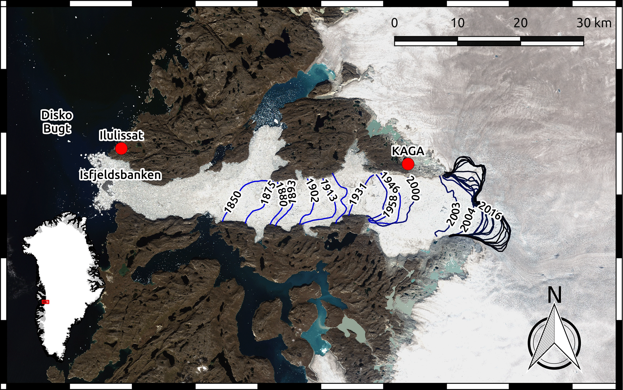
Figure 1Glacier front positions of Jakobshavn Isbræ from Khan et al. (2015) (1850–1985) and CCI products derived from ERS, Sentinel-1 and Landsat data by ENVO (1990–2016). The background map is a Landsat-8 image from 16 August 2016 (from the U.S. Geological Survey). Location names that occur in the text are marked. The inset shows the location of Jakobshavn Isbræ in Greenland.
The aim of this study is to investigate the external, glaciological and geometric controls on Jakobshavn Isbræ in response to a linear forcing on a centennial timescale. We use a simple numerical ice flow model (Nick et al., 2010; Vieli and Payne, 2005) with a fully dynamic treatment of the calving front to assess the relative impact of fjord geometry and climate forcing on the retreat of Jakobshavn Isbræ from the LIA maximum to the present day. Geometric controls are isolated by (a) using a linear forcing to avoid complex responses and (b) artificially straightening the trough width and depth. The model experiments are run over several centuries to account for internal glacier adjustment. The application of the model on a real glacier enables a comparison of model results with long-term observed velocities and front positions, but also ensures the use of realistic values for the width–depth ratio and the model parameters.
Section 2 documents the numerical ice flow model, followed by an outline of the specific model setup used for the simulations in Sect. 3. Section 4 describes the results of the experiments with varying climate forcing and fjord geometry. The importance of trough width versus depth and forcing is discussed in Sect. 5, followed the limitations of the model and the implications of our results for understanding the past.
We use a dynamic depth- and width-integrated numerical ice flow model constructed for marine-terminating glaciers (Nick et al., 2009, 2010; Vieli and Payne, 2005; Vieli et al., 2001). Despite many assumptions required, this model is well suited to study the long-term (centennial) retreat pattern of an outlet glacier with high basal motion (such as Jakobshavn Isbræ). It is based on mass continuity and a balance between the driving stress, longitudinal stress gradient, and basal and lateral drag. The model benefits from a robust treatment of the grounding line (Pattyn et al., 2012) consistent with Schoof (2007) and a fully dynamic marine boundary (Nick et al., 2010). It is also more efficient than complex models (Bondzio et al., 2016; Muresan et al., 2016), which enables multiple model runs covering several centuries. The physical calving law applied in the model has been successfully tested on several outlet glaciers where there are observational data available (Nick et al., 2013). The calving law also has the advantage of allowing for a dynamic and free migration of the glacier terminus, given changes in climate forcing. The climate forcing is implemented as a slow linear change in surface mass balance (SMB), crevasse water depth, submarine melt and buttressing by sea ice – model parameters that represent the impact of changes in temperature. In this section, the physical approach, parameterizations and the implementation of climate forcing are described.
2.1 Numerical ice flow model
The numerical ice flow model as described in Nick et al. (2010) calculates the time-varying ice thickness H from the along-flow ice flux and mass balance, using a depth- and width-integrated continuity equation:
U is the width- and depth-averaged velocity, t the time and x the along-flow component. The width W is assumed to be symmetric around the central flow line. The mass balance includes the surface mass balance and submarine melt below the floating tongue (described in Sect. 2.3).
The ice flux is controlled by a balance of lateral and basal resistance, along-flow longitudinal stress gradient and driving stress. Lateral resistance is parameterized using a width-integrated horizontal shear stress (van der Veen and Whillans, 1996) and we use a Weertman-type basal sliding law based on effective pressure (Fowler, 2010). The longitudinal stress gradient is dependent on the effective viscosity ν, which is nonlinearly dependent on the longitudinal strain rate and the rate factor A (Nick et al., 2010). The stress balance is calculated as
where s is the surface elevation; g is the gravitational acceleration; D is the depth of the glacier below sea level; and ρi and ρs are the densities of ice and ocean water, respectively. n and m are the exponents for Glen's flow law and sliding relations, respectively. The lateral enhancement factor E, controlling the lateral resistance, and the basal sliding parameter As are model parameters that are adjusted to roughly match the observed ice flow and thickness for the present fjord geometry. Both parameters are constant along the flow line and in time. The dependency of the basal resistance on effective pressure is accounted for through the term .
The grounding line position is calculated with a flotation criterion based on hydrostatic balance (van der Veen, 1996). Its treatment relies on a moving grid: at each time step the grid adjusts freely to the new glacier length, continuously keeping a node at the calving front (Nick et al., 2009, 2010; Vieli and Payne, 2005). This allows for a precise simulation of the glacier front and grounding line position using high grid resolution. The grid size is Δx = 302 m initially and reduces to Δx = 292 m at the present-day position due to the use of a stretched grid. At the marine terminus, a dynamic crevasse-depth calving criterion is used as described in Sect. 2.2.
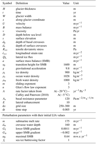
Cuffey and Paterson (2010)Table 1List of variables, physical parameters and constants used in the model. The forcing parameters with their initial (LIA) values are given in the lower part. Parameter values used for the glacier retreat experiments are listed in Table 2.
2.2 Calving law
The fully dynamic crevasse-depth criterion calculates calving where the sum of surface and basal crevasse depth (ds and db, respectively) penetrates the whole glacier thickness (Nick et al., 2010). The depth of the surface crevasses is given by
The depth of the surface crevasses is calculated from the tensile deviatoric stress Rxx and the pressure from melt water filling up the crevasses (Eq. 3) (Nick et al., 2010; Nye, 1957). Note that the water depth in crevasses dw is not a physical quantity, but a forcing parameter within the calving model that links calving rates to climate. ρw is the density of freshwater. The tensile deviatoric stress is the difference between tensile stresses that pull a fracture open and the ice overburden pressure. It is calculated via Glen's flow law from the longitudinal stretching rate , which is responsible for the opening of crevasses by
which depends on a sea ice factor fi, accounting for reduced buttressing due to weakening of ice mélange. The depth of basal crevasses is calculated from tensile deviatoric stresses and the height above buoyancy (Nick et al., 2010):
Water in crevasses and sea ice buttressing are both model parameters that impact the glacier response by changing the calving rate. Because the parameters are linked to different processes, they are kept separate in the model to enable a distinct forcing.
2.3 Atmosphere and ocean forcing
The model SMB, a, is derived from observed monthly mean SMB data at Jakobshavn Isbræ (Box, 2013). The SMB data are based on a combination of meteorological station records, ice cores, regional climate model output and a positive degree-day model. Its implementation in our model consists of a piecewise linear function of surface elevation separated by a transition height s0: in the steep lower part of the glacier, the SMB increases with elevation; and, in the flat upper part of the glacier, where the precipitation is low, the SMB decreases with elevation (Eq. 6).
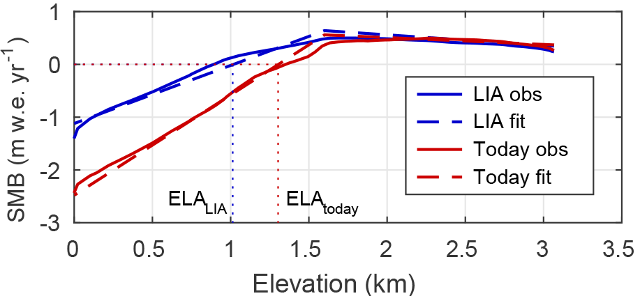
Figure 2SMB profiles along Jakobshavn Isbræ's main flow line at the LIA (1840–1850 average) and present day (2002–2012 average) from observations by Box (2013) and the linear fit used in the model. Thin dotted lines show position of the equilibrium line altitude (ELA) for the present-day and LIA fit.
Figure 2 shows the observed and estimated linear SMB profiles for the LIA (1840–1850 average) and for the present day. The corresponding values for the vertical gradients Gl and Gu as well as the SMB a0 at the height s0 are given in Tables 1 and 2.
Submarine melt is implemented in the model as a vertical melt rate that decreases the glacier thickness seaward of the grounding line and is assumed to be spatially uniform. The induced artificial step decrease in ice thickness at the grounding line is smoothed out in the model by a sufficiently small time step. The submarine melt rates are one order of magnitude smaller than the grounding line flux. Sensitivity analyses with along-flow variations in submarine melt (Motyka et al., 2011) show similar results, as long as the constant submarine melt rate is comparable to the along-flow averaged submarine melt rate.
2.4 Lateral ice flow
The model domain covers the full drainage basin towards the ice divide at about 520 km upstream of the present-day position. For the lowermost 77 km, we restrict the model width to the pronounced narrow channel seen in bed topography data to realistically account for lateral and basal stresses. Lateral ice flow into this narrow channel from the surrounding ice sheet and tributary glaciers is implemented as an additional SMB similar to previous studies (Jamieson et al., 2014; Lea et al., 2014; Nick et al., 2013), giving a realistic mass flux into the lower channel. This lateral influx QL,0 is initially calculated as the sum of the northern and southern lateral fluxes. These are given by the observed ice velocity UL,0 and thickness HL,0 (Morlighem et al., 2014; Rignot and Mouginot, 2012) at each grid point along the lateral boundary of the narrow main channel, divided by the width of the main trough WJI (Eq. 7). The strength of the initial influx is indicated by the arrows in Fig. 3 and locally accounts for about 100 times the SMB, with a maximum of 120 m yr−1.
We assume that the relative contribution of the lateral flux to the overall flux is constant in time; therefore, we scale it with the change in the overall flux with time (Eq. 8).
QJI,0 and QJI,t are thereby the initial overall flux through the main trunk and the flux after time t, respectively. Note that the constant relative contribution by side fluxes is a rough approximation. A thinning of the main trunk could initiate a speed-up in the tributary glaciers due to increased surface slope.
Despite the general focus of this study on the external versus geometric controls on glacier retreat, we apply the model to Jakobshavn Isbræ – a well-studied glacier on west Greenland. The intention is to use a realistic along-flow glacier geometry to compare modeled ice thickness, length and velocity with observations.
Observations of ice velocities, calving front positions, ice thickness and ice discharge (Howat et al., 2014; Joughin et al., 2004, 2014; Khan et al., 2015) are used to tune model parameters. In the following, we distinguish between constant parameters (basal sliding, rate factor and lateral enhancement factor) and climate-related perturbation parameters (SMB, submarine melt rate, crevasse water depth and sea ice buttressing). For the model experiments, the perturbation parameters are changed linearly from their LIA values to simulate increasing temperatures. Importantly, the calving front and grounding line evolve freely during retreat. Only combinations of forcing parameters that simulate a total retreat rate matching the observed retreat of about 43 km from the LIA to 2015 are considered. In the following, the choice of tuning parameters and the perturbations are described, together with relevant observations.
3.1 Model glacier geometry
Jakobshavn Isbræ extends 520 km inland towards the ice divide and can be distinguished from the surrounding ice sheet by its high velocities along the deep trough. The geometry of the model glacier consists of a narrow (in average about 5.4 km wide) and deep (1.3 km at the deepest) trough; further upstream, it widens gradually with a relatively flat and shallow bottom. The fjord width in today's ice-free area is obtained from satellite images (Fig. 1). The channel width in the fast-flowing part (77 km upstream of the 2015 position) is defined as the trough width at the present-day sea level from topography data by Morlighem et al. (2014). Further upstream, where the catchment widens gradually, the width is defined following Nick et al. (2013). For the one-dimensional glacier depth in the deep trough and fjord, we use the along-flow bed topography profile as it is presented in Boghosian et al. (2015). The fjord bathymetry is obtained from Operation IceBridge gravity data and the subglacial trough profile from high-sensitivity radar data by Gogineni et al. (2014). For the bed in the wider catchment area, 150 m resolution data by Morlighem et al. (2014) are averaged over the glacier width.
3.2 Constant parameters
Most observations only exist for the present day. Parameters that are constant in time (basal resistance, lateral enhancement factor and rate factor) are tuned with observations to obtain a steady-state glacier corresponding to the observed present-day glacier geometry. After tuning the constant parameters, the climate-related perturbation parameters are reduced to colder temperatures to achieve an initial steady state corresponding to the observed LIA front position. For the LIA steady state, the only constraints are given by the LIA front position (Khan et al., 2015) and the height of the LIA trimline found at the GPS station KAGA (Jeffries, 2014) by Csatho et al. (2008).
Basal sliding – as implemented in the model – influences ice flow and hence the surface slope and thickness. The basal sliding parameter is chosen to achieve an observed present-day thickness of 3065 m at the ice divide (Howat et al., 2014); the present-day thickness in the interior is also valid for the LIA initialization as the ice sheet is assumed to be in a steady state above 2000 m of elevation within this time period (Krabill, 2000). We keep the basal sliding parameter constant in time, because the impact of increased melt on basal sliding on interannual timescales is still unclear (Sole et al., 2011; Tedstone et al., 2015). Also, the model takes into account the dependency of basal sliding on the effective pressure, which is calculated explicitly. The actual degree of basal resistance at the bed of Jakobshavn Isbræ is highly debated, with some studies explaining high surface velocities as reflecting a slippery bed (Lüthi et al., 2002; Shapero et al., 2016), whereas other studies ascribe the high velocities to weakened shear margins (van der Veen et al., 2011), or an interplay of both processes (Bondzio et al., 2017).
The surface profile and ice velocity are determined by the lateral resistance and the rate factor. A uniform lateral enhancement factor is applied along the entire glacier, controlling the strength of the transmission of lateral drag to the sides. A value of E=10 gives a simulated present-day surface with a best fit to observations (Howat et al., 2014). The rate factor for Glen's flow law is to a first approximation a function of ice temperature. Here it is set to values corresponding to temperatures of −20 ∘C at the ice divide, linearly increasing to −5 ∘C at the terminus (Cuffey and Paterson, 2010). This gives a good fit of simulated present-day glacier surface and ice velocities to observations (Howat et al., 2014; Joughin et al., 2014). The rate factor is kept constant in time.
3.3 Forcing experiments and perturbation parameters
The climate-related perturbation parameters are tuned for the LIA steady state to simulate the observed glacier length and velocities, or the ice discharge. Starting from the initial LIA glacier configuration, a retreat is triggered by simultaneous linear changes in SMB, crevasse water depth, submarine melt rate and sea ice buttressing. The parameter perturbations are combined in order to obtain a total retreat of 43 km from 1850 to 2015, corresponding to the observed retreat. Nine different parameter combinations that satisfy the observational data, and cover a wide range of perturbations, are presented here. Table 2 shows the parameter values reached by the year 2015 in the nine different model runs.
SMB is the only purely physical and well-known variable both for LIA and today (Box, 2013). The piecewise linear function presented in Sect. 2.3 is a good approximation to the observed profiles (Fig. 2) and is therefore used here. All model experiments use the same gradual changes of the SMB gradients and maximal SMB from the LIA values to present-day values (Table 2).
Submarine melt is influenced by ocean temperatures. In Disko Bugt, ocean temperatures have increased from about 1.5 ∘C in 1980 to 3 ∘C in 2010 (Lloyd et al., 2011), including a 1 ∘C warming in 1997 (Hansen et al., 2012; Holland et al., 2008). Jenkins (2011) estimates a doubling of melt rates underneath the floating tongue of Jakobshavn Isbræ (depending on initial conditions and the way in which melting is applied), when considering a 1 ∘C warming and steepening of the glacier front. Submarine melt rates may be additionally enhanced by increased subglacial ice discharge (Jenkins, 2011; Sciascia et al., 2013; Xu et al., 2012, 2013), although this may be a local effect and negligible when width averaged (Cowton et al., 2015). Observations of submarine melt rates beneath Jakobshavn Isbræ's floating tongue suggest an annual melt rate of 228 ± 49 m yr−1 between 1984 and 1985 (Motyka et al., 2011) and 2.98 m d−1 (1087 m yr−1) averaged over the melt seasons in 2002 and 2003 (Enderlin and Howat, 2013). Since the submarine melt rate is otherwise poorly constrained, especially further back in time, we employ a large range of linear forcing, from no increase to a 2-fold increase in the LIA value of 175 to 340 m yr−1 in 2015. Note that the model neglects submarine melt at the vertical calving front.
The crevasse-water depth has not been measured and is applied as a nonphysical model parameter regulating discharge fluxes. It is likely to be exaggerated in the model, accounting for the lack of submarine melt at the vertical glacier front. For the LIA steady state, the crevasse water depth is set to 160 m, which produces a calving rate of 34 km3 yr−1 in 1985 after the applied linear forcing. This is the same order of magnitude as the observed calving rate of 26.5 km3 yr−1 in 1985 (Joughin et al., 2004), as well as the more recent values between 24 and 50 km3 yr−1 (Cassotto et al., 2015; Howat et al., 2011; Rignot and Kanagaratnam, 2006). The increase in crevasse water depth with time is unknown, but may be related to runoff, which has increased by 63 % since the LIA (Box, 2013). To account for such a large range, we increase the crevasse water depth from its LIA value to values between 185 and 395 m in 2015. The crevasse water depth is tuned depending on the combination of sea ice buttressing and submarine melt rate to reach the observed retreat (Table 2).
Ice mélange in the fjord can apply a buttressing stress to the calving front of about 30–60 kPa, or one-tenth of the driving stress (Walter et al., 2012). With increasing air and ocean temperatures, ice mélange can weaken or break up, thereby influencing iceberg calving (Reeh et al., 2001; Sohn et al., 1998). However, the correlation between ice mélange and iceberg calving is poorly known. Breakup of ice mélange is thought to impact frontal migration on a daily to seasonal timescale, leaving annual fluxes unaffected (Amundson et al., 2010; Cassotto et al., 2015; Todd and Christoffersen, 2014; Todd et al., 2018; Walter et al., 2012). We conduct experiments with unchanged buttressing by sea ice (fs=1; also used for the LIA steady state), as well as decreased buttressing by a factor of 2 and 3 compared to the LIA value in 2015.
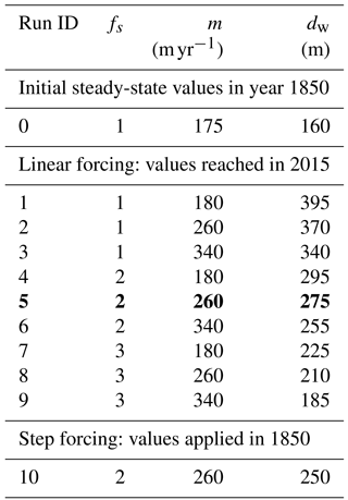
Table 2Nine combinations of the perturbation parameters used in this study. Values shown here are those reached in 2015 after a linear perturbation from their LIA value shown in Table 1. Values for the SMB are perturbed to the same 2015 values for all model runs: , , . Run 5 (in bold) is presented in more detail in the paper.
The observed retreat position in 2015 is reached with all the parameter combinations presented in Table 2. The 2015 values for each parameter depend on the values for the other parameters. This means, for example, that in the case of reduced sea ice buttressing and a small crevasse water depth, a low submarine melt rate is needed. Similarly, if sea ice buttressing is high and submarine melt is low, the crevasse water depth must be large.
In addition to experiments with linearly increased parameters, we also conduct one experiment with a step increase in the four parameters starting from the LIA maximum. The step increases in sea ice buttressing, submarine melt rate, crevasse water depth and SMB applied starting at 1850 are comparable to those reached in the model year 2015 in run 5, with slightly different values to reach the right front position in 2015. All experiments shown in Table 2 are run until 2100 in order to test the temporal and spatial response to the underlying geometry.
Despite a relatively high number of frontal observations since the LIA (Fig. 1), only the observed calving front positions in 1850 and 2015 are used to tune the model parameters; in between these two time slices, the forcing parameters increase linearly and the glacier length evolves freely. We present the time evolution of the simulated front positions together with observations. To obtain one-dimensional observed front positions, we assume the trough to be approximately east–west oriented. We calculate the mean latitudinal coordinate of each observed calving front (Fig. 1) with the corresponding longitudinal position at that latitude. The positions of the resulting one-dimensional front positions lie approximately in the center of the trough. The uncertainty of the front positions is calculated as the maximal spread of each front in cross-trough direction.
3.4 Geometric experiments
In addition to the effect of climate forcing, we investigate the effect of fjord geometry and the relative importance of bed topography versus channel width. The experiments are designed with a smoothed width and depth in the deep and narrow trough. Four different geometry combinations are constructed and shown in Fig. 3.
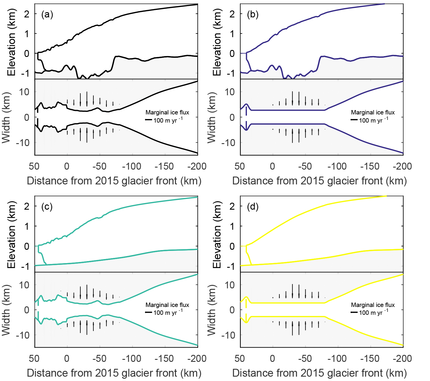
Figure 3Different model geometries used to investigate the impact of topography on ice dynamics. (a) Original geometry, (b) straight width, (c) straight bed, and (d) straight width and bed. Arrows indicate the tributary ice flux, with their length representative for the influx volume.
-
Original geometry: observed width and depth of the trough as described in Sect. 3.1.
-
Straight width: the width until 80 km inland of today's front is set to a constant value of 5.4 km. Only at the LIA front position, a wide section is kept in order to reach a steady state with the same parameters. The depth is kept as in a.
-
Straight bed: the bed of the deep trough to 120 km inland of today's front is smoothed to get an almost straight bed, linearly rising inland. The width is kept as in a.
-
Straight width and bed: both the width and the bed are straight.
The runs with simplified geometry start from a steady state at the LIA front position with the same parameters and forcing as for the original model setup (Table 2). Due to the changed topographies, the glacier surfaces and velocities differ from the original geometry and the LIA front position is slightly changed.
In this section, we present the steady-state glacier at the LIA maximum extent and the glacier retreat simulated with run 5 (Table 2) as an example. In addition, the response to different forcing parameter combinations, more simplified geometries and a step forcing are presented.
4.1 Jakobshavn Isbræ at the LIA maximum
The initial steady-state glacier as shown in Figs. 3a and 5a is reached with the parameters in Table 2. The glacier has an uneven surface that reflects the trough geometry, which is common for fast-flowing ice streams (Gudmundsson, 2003). At the position of KAGA, the surface elevation reaches about 400 m compared to the 300 m of the LIA-trimline height (Csatho et al., 2008); however, the side margins are expected to be lower than the centerline and the model glacier has a – probably overestimated – surface bump at this position. The LIA glacier terminates with a 9 km long floating tongue, where it has a velocity of 5 km yr−1 and a grounding line flux of 35 km yr−1. The modeled width-averaged basal shear stress for the LIA is about 128 kPa at 40 km inland of the present-day front position and the driving stress is 290 kPa at the same location, when applying a 3 km moving average to smooth the surface bumps. In comparison, other modeling studies obtain lower basal resistance (Habermann et al., 2013; Joughin et al., 2012) and data assimilation methods imply basal stresses at the bed of the deep trough of about 65 kPa at 50 km upstream of the calving front, equivalent to only 20 % of the driving stress (Shapero et al., 2016). However, these estimates are from the present day and it is unknown how much the relative contribution of the stresses has changed over the time period. During the speed-up, the basal shear stress might have been reduced in the lowermost 7 km, and not changed further upstream (Habermann et al., 2013). Note also that the stresses provided by the model are width averaged.
4.2 Nonlinear glacier response to linear forcing
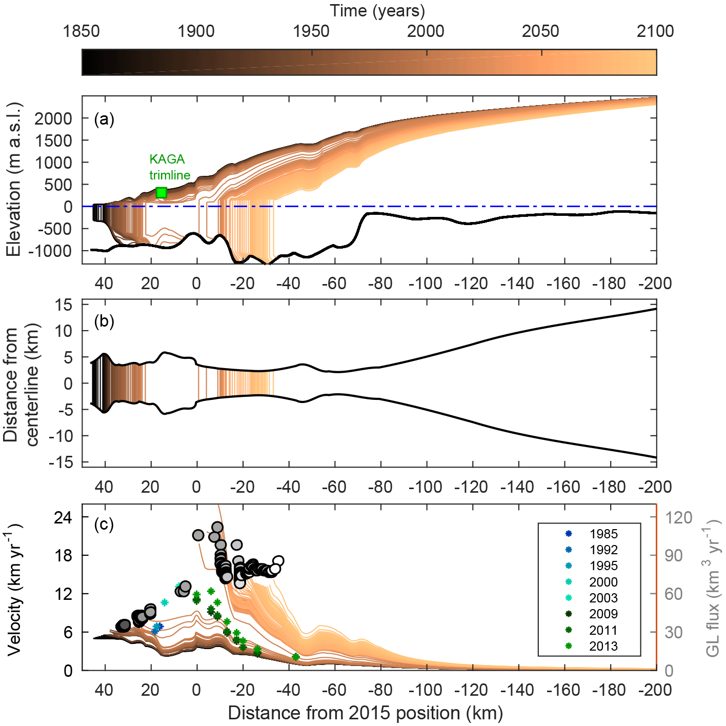
Figure 4Modeled retreat of Jakobshavn Isbræ in response to a gradual change of the forcing parameters (run 5 in Table 2). Yearly profiles are shown for (a) the along-flow glacier profile and the elevation of the KAGA LIA trimline (Csatho et al., 2008) in green, (b) the front positions in a top view and (c) the along-glacier annual velocities including the yearly grounding line (GL) flux (gray circles from dark to light with time). Observed yearly velocities are plotted at the calving front from 1985 to 2003 (Joughin et al., 2004) and at seven different points upstream from the glacier front from 2009 to 2013 (Joughin et al., 2014).
Figure 4a and b show that the modeled front position retreats nonlinearly in response to the linear external forcing (shown here is run 5 in Table 2). It retreats 21 km during the first 163 years, after which a 16 km long floating tongue forms. During the break-off of the tongue in 2013 to 2014, the front retreats a further 23 km. Throughout the retreat, the glacier terminus alternates between a floating tongue and a grounded front. The front velocities (Fig. 4c) only increase by 3 km yr−1 during the first 163 years and more than double from 8 to 19 km yr−1 when the floating tongue breaks off. This acceleration is overestimated, as the simulated tongue breaks off faster than observed. However, velocity observations by Joughin et al. (2004, 2014) shown in Fig. 4c are smaller than that simulated in the early 1990s but are in between the simulated velocities before and after the break-off. The model simulations show that the acceleration continues until the retreat of the front slows down. The grounding line flux, calculated as the grounding line velocity times the grounding line gate area, increases from 35 to 65 km3 yr−1 from the LIA until 2015 compared to observed values of about 32–50 km3 yr−1 between 2005 and 2012 (Cassotto et al., 2015; Howat et al., 2011; Rignot and Kanagaratnam, 2006). Beyond 2015 it increases to 100 km3 yr−1 and finally stagnates at a flux of 77 km3 yr−1.
The various parameter combinations presented in Table 2 – and many more that are in between those presented here – reproduce the observed total retreat since the LIA. Figure 5 shows the retreat of the glacier front and grounding line with time for the nine parameter combinations applied. The simulated temporal retreat pattern of the glacier front is similar for all experiments and shows the strong nonlinearity of the frontal retreat – despite the linear forcing (Fig. 5a). The response to the different forcing experiments differs mainly in the timing of the phases of rapid retreat, especially the final retreat just after 2050. All model runs show a very abrupt retreat of at least 23 km within a few years, which corresponds to the observed retreat of 19 km after year 2000. The simulated frontal positions differ from those observed, which is expected due to the strong simplification of the forcing. The aim here is to study the geometric controls on rapid retreat, rather than tuning the model until the simulated retreat fits the observations. The reasons for the deviation of the simulations from the observations are discussed in Sect. 5.
The grounding line retreats in a more stepwise manner (Fig. 5b) compared to the glacier front. Before 2015, it stabilizes at distances of 32, 25 and 20 km from the 2015 frontal position for all experiments. It retreats more gradually beyond 2015 with short still-stands at 8, 12 and 18 km upstream of the present-day position. The forcing parameter combination thereby determines the timing of the grounding line displacement.

Figure 5Simulated position of (a) the front and (b) the grounding line (GL) for nine different gradual forcing combinations presented in Table 2. The colors for the different model runs are random. Black dots show the observed front positions at the centerline with a spread (gray shading) corresponding to the across-fjord variation of each front position (Fig. 1).
4.3 Control of fjord geometry on front and grounding line retreat
The residence time of the grounding line is analyzed for the different geometries introduced in Fig. 3. Residence time is thereby quantified by the amount of time that the grounding line rests within a distance of 1 km. Figure 6a shows the original geometry with the most pronounced pinning points at distances of 32, 25, −10 and −13 km from the 2015 position. Only the length of grounding line still-stand thereby varies among the nine different model runs (Table 2), whereas the pinning point locations coincide (also seen in Fig. 5b). Artificially straightening the width removes the pinning points at 25 km and those beyond the 2015 position (Fig. 6b). Instead, the glacier rests at the present-day position. The geometry with the straightened bed causes a similar response to the linear forcing as with the original geometry, only with a wider spread of pinning points (Fig. 6c). Straightening the bed and the width removes all pinning points (Fig. 6d) and leads to a linear retreat. Note that all geometries have an initial pinning point at the LIA position to allow a steady state at the LIA position. Generally, a reduction in the complexity of the fjord geometry, for example, straightening the bed and/or width, reduces the number of pinning points.
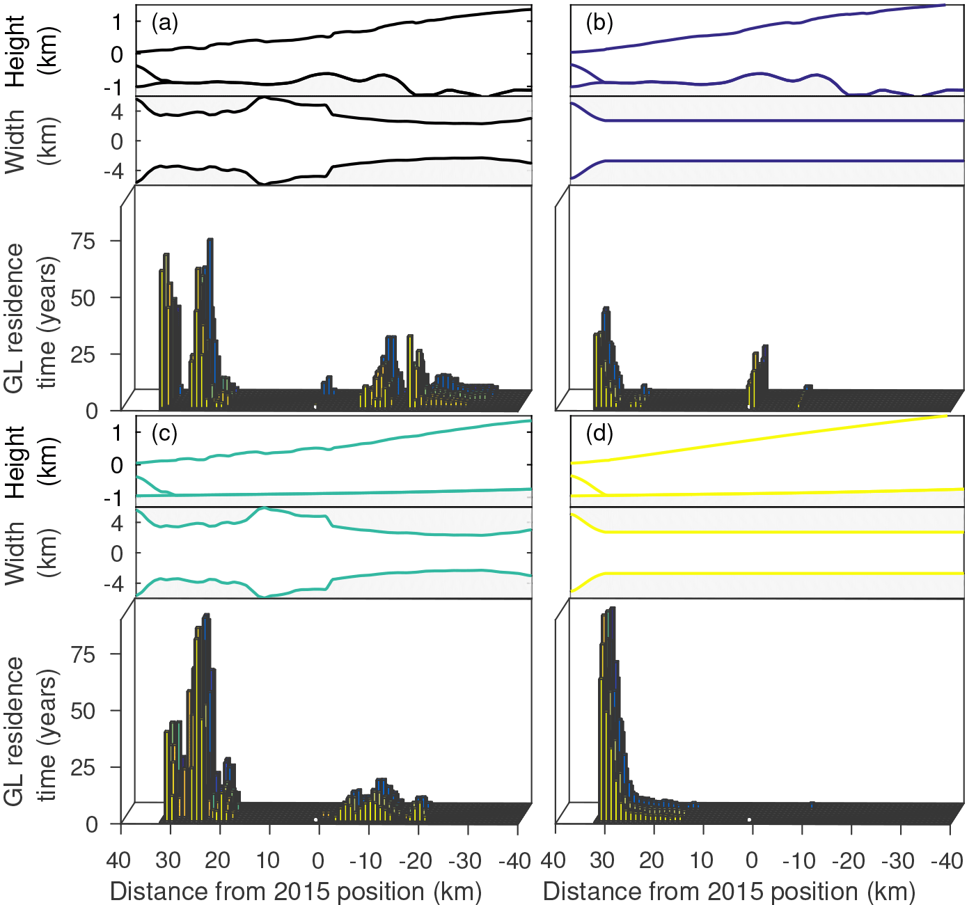
Figure 6Residence time of the grounding line (GL) for the different geometries presented in Sect. 3.4: (a) the original geometry, (b) straightened width, (c) straightened bed, and (d) straightened width and bed. The bars represent the time that the grounding line rests within 1 km, and the colors correspond to the model runs in Table 2. Only residence times of more than 2 years are included.
4.4 Delayed abrupt glacier response
In addition to the linear increase in climate forcing, the response to a step forcing (Table 2) is presented in Fig. 7. With the step forcing, the glacier front remains at a distance of 22 km for 60 years, before it retreats rapidly to its new pinning point. This unprovoked rapid retreat – after centuries of constant forcing – demonstrates the long response time of the glacier (Bamber et al., 2007; Enderlin et al., 2013; Jóhannesson et al., 1989; Nye, 1960). The long response time is caused by a slow adjustment of the glacier volume to external changes. The corresponding accumulated volume loss, also shown in Fig. 7, adjusts steadily to the initial changes in forcing, despite the constant grounding line position. During the rapid frontal retreat, the volume decreases by 300 Gt and continues even after the grounding line reaches a still-stand. This emphasizes that a constant grounding line position does not imply a steady state. Similarly, an observed rapid retreat of a marine-terminating glacier might be the delayed response to historic temperature changes.
For the example of Jakobshavn Isbræ, our results show the importance of lateral and basal topography and their implications for the evolution of glacier retreat in fjords. This knowledge can be used for a better understanding of the recent observed retreat history; however, it is hard to isolate the relative impact of changes in ocean forcing, SMB and internal factors including the fjord geometry. Here, we discuss the impact of fjord geometry on glacier front retreat and compare the simulated glacier response to the recorded long-term glacier retreat history. In addition, we explore the implications of our results for the future response of Jakobshavn Isbræ to changes in climate.
We argue that fjord geometry, and in particular fjord width, to a large degree dictates the retreat history of marine-terminating glaciers. Nevertheless, changes to the external forcing of the glacier are important, because their magnitude controls the onset and overall rate of the retreat (Fig. 5).
5.1 Geometric control on glacier stability
Our simulations show that once a glacier retreat is triggered, through changes at the marine boundary, or at the glacier surface, a nonlinear response unfolds due to variations in the fjord geometry with a complexity given by the bed topography and the trough width. For a retrograde bed, where water depth increases as the glacier retreats, the ice discharge increases, leading to further unstable glacial retreat in the case of constant lateral stresses (Schoof, 2007; Weertman, 1974). Previous studies show that changes in the width of a glaciated fjord impact the lateral resistance as well as the ice flow, thereby stabilizing the glacier where narrow sections occur (Enderlin et al., 2013; Gudmundsson et al., 2012; Jamieson et al., 2012, 2014; Morlighem et al., 2016; Åkesson et al., 2018). These findings are corroborated by our model results. However, most of these earlier studies use synthetic glaciers that do not allow for a validation of the model against observations. Further, the shorter time periods considered neglect the long-term adjustment of the glaciers. Figure 7 shows that the timescale of glacier adjustment can be several decades. However, in reality temperature changes are likely smaller and less abrupt than we have imposed. Nevertheless, our study demonstrates that the observed recent retreat could have been triggered and sustained by an earlier warm event. This finding is consistent with Jamieson et al. (2014), who studied Antarctic ice stream retreat on millennial timescales. Depending on the local geometry of the underlying bed, individual glaciers exhibit different response times and spatial extensions of dynamic thinning (Felikson et al., 2017).
The geometry experiments in Fig. 6 assess the relative role of glacier width versus glacier length on Jakobshavn Isbræ. The width seems to be the leading factor for grounding line still-stand, as artificially straightening the fjord removes the pinning points that cause a slowdown of the grounding line retreat. Flattening the bed topography is less efficient in linearizing the grounding line retreat compared to straightening the fjord. It has to be considered that the glacier trough is an order of magnitude wider than it is deep, with larger variations in the width compared to the bed, increasing the importance of the glacier width.
5.2 Relative role of forcing parameters
Only certain parameter combinations simulate the observed retreat pattern of Jakobshavn Isbræ since the LIA (Table 2). If the submarine melt rate is increased, the crevasse water depth has to be reduced and/or the sea ice buttressing increased. Similarly, if the sea ice buttressing is reduced, the crevasse water depth and submarine melt rate have to be smaller (Table 2). Importantly, none of the forcing parameters can trigger the retreat alone, unless the change to the parameter is unreasonably large relative to its LIA value. Changed individually, the submarine melt rate would have to reach 650 m yr−1 in 2015 – an increase of 370 % from the LIA, the crevasse water depth has to increase to 400 m (250 % larger than the LIA value), and the sea ice buttressing factor has to be more than quadrupled (value 4.2 relative to LIA factor of 1) in 2015 to force a strong enough retreat. Absolute values for the parameters have to be taken with caution, as they do not necessarily correspond to physical variables. For example, to reach the observed grounding line flux, the value for the crevasse water depth is likely too high in our study. This is because it is a parameter for calving that has to balance the neglected submarine melt along the calving front in the model. The change in parameters required to trigger the retreat is also dependent on the initial parameter choices and what forcing is needed to unpin the grounding line from the initial pinning point. As shown by Enderlin et al. (2013), non-unique parameter combinations can exist for the same front positions. This implies that real-world observations are vital to reduce uncertainty in transient model simulations.
Note that the SMB contribution to the frontal retreat is insignificant, even if the lower SMB gradient Gl is doubled and the SMB curve is lowered by 50 %. Taken together this gives a SMB at the terminus of −6 compared to −1.1 during the LIA (cf. Fig. 2). In our model of Jakobshavn Isbræ, variations in air temperatures contribute mainly through runoff and the filling of crevasses with water, rather than directly through surface ablation. For the specific geometry of Jakobshavn Isbræ, the influx of ice at the lateral boundaries is a factor of 100 larger than the local SMB and could be important for the sensitivity of the glacier to changes in climate forcing. However, the lateral influx is an order of magnitude smaller than the flux through the main trough and a sensitivity study shows that the lateral flux has a minor impact on the retreat pattern (not shown here). If all other parameters are kept fixed, the lateral influx has to decrease by nearly 70 % from its LIA value in order to simulate the observed retreat.
5.3 Model limitations and comparison to observations
In order to isolate the effect of geometry on glacier retreat, a relatively simple – but physically based – model is forced with a linearly changing external forcing. Notwithstanding a number of assumptions, the model is well suited, as it is computationally inexpensive and allows for a large set of ensemble simulations starting from the LIA in 1850. Studying long time periods is vital in order to capture internal glacier adjustments to changes in external forcing beyond the last few decades. Unfortunately, few observations exist to validate the model for such a long time period, which supports our chosen idealized model setup. The model parameters are calibrated with the few observations that exist, and the modeled retreat of Jakobshavn Isbræ is compared to the observed retreat.
Both modeled and observed calving front positions show a highly nonlinear retreat and the rapid disintegration of a several-kilometer-long floating tongue (Fig. 5). The model results show a robust dependency of this nonlinear retreat on the trough geometry, especially the trough width. However, the modeled glacier front retreats more slowly (deviating up to 13 km from the observations) and exaggerates the break-off of the floating tongue. For the dynamic interpretation of the nonlinear retreat, a perfect agreement is not essential, especially given the one-dimensionality of the model and the uncertainties in the width-averaged observed front positions.
For the interpretation of the model results, the assumptions made in the model have to be considered. The most obvious assumption is the one-dimensionality that does not account for across and vertical variation in geometry. The residence time of the grounding line at pinning points may be partly overestimated due to this width and depth integration. Local bedrock highs that partly pin the floating tongue (Thomas et al., 2003) are not properly represented in a width-averaged setting, and the width is regarded as symmetric around the central flow line. In reality, one lateral margin might narrow down and pin the grounding line while the other lateral margin widens up, causing an asymmetric calving front retreat (Fig. 1). Here, we only focus on the large-scale dynamics; lateral and vertical variations in the ice flow are seen as second-order processes, considering the high basal motion and high velocities in the deep and narrow channel at the lowermost 100 km of the model domain. As the glacier retreats further upstream “into” the ice sheet, the lateral ice flux becomes more significant and the whole drainage area should explicitly be modeled, favoring the use of a three-dimensional model for future projections.
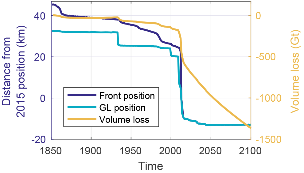
Figure 7Simulated front and grounding line (GL) positions with accumulated volume loss for the step forcing (Table 2).
The depth and width integration also applies to internal glacier properties; ice temperatures are in reality high at the bottom (Lüthi et al., 2002), so most deformation happens there, whereas the model assumes a vertically constant shearing and a constant rate factor. Along the margins of a real glacier, ice viscosity drops significantly in response to acceleration and calving front migration (Bondzio et al., 2017), and marginal crevasses can form, which are not considered here. However, lateral drag and weakened margins mostly affect the timing and not the details of the retreat, as has been tested in an idealized setting with the same model (Åkesson et al., 2018). Ice viscosity is a response to dynamic changes rather than a cause, and it is therefore not expected to change the retreat pattern significantly. However, ice viscosity may slightly alter the timing and residence time of the grounding line.
Several parameterizations of physical processes are used in the model, such as submarine melt and buttressing by ice mélange. This complicates direct model validation with observed values. However, these processes are still crudely implemented, if at all represented in glacier models. For example, many models prescribe the position of the calving front (Bondzio et al., 2017), or only focus on grounding line migration, whereas our model uses a physical calving law. Also, few observations exist of submarine melt, calving rates and basal sliding, especially over the long time period studied here. The impact of plume dynamics on submarine melt could be implemented in our model (Jenkins, 2011), or an along-flow variation in submarine melt rate (Motyka et al., 2003). However, the number of observations on ocean temperatures is sparse and the model results are similar when using along-flow variations in submarine melt, compared to a constant value along the floating part (not shown here). Also interannual variability of calving rates due to submarine melt, runoff and ice mélange is neglected and not considered as important when looking at centennial timescales. Although many of the model parameters are only indirectly linked to observations, existing observations such as velocities, ice discharge and thickness are used to tune the parameters and to reproduce the glacier behavior as close as possible. Note that the change in forcing parameters required to dislodge the grounding line from its stable LIA position might be overestimated, due to large variations in bed topography and width. Also, many parameter combinations can simulate the same stable position but lead to different glacier retreat (Enderlin et al., 2013). Therefore, we include a large range of parameter perturbations, leading to different residence times for the grounding line, but with no reduction in the importance of the geometry in defining locations of intermittent slowdown in the overall grounding line retreat.
The choice of the model is dependent on the questions raised; if the objective is to accurately predict or reconstruct the time evolution of glacier retreat (Muresan et al., 2016; Nick et al., 2013), a more sophisticated model has to be used. Note that also the observations contain uncertainties. The front position can vary by several kilometers seasonally (Amundson et al., 2010) and this position varies by several kilometers across the trough (Fig. 1). For the calculation of the one-dimensional front position, we assume a west–east orientation of the trough, which gives an offset at the most recent calving fronts; however, the deviation is only a few kilometers and within the spread of the across variation of the calving front. Most importantly, the bed topography – especially in the densely ice-covered fjord and a sediment-rich subglacial bed (Boghosian et al., 2015) – is challenging to obtain. Due to the strong control of the fjord geometry on the glacier retreat, small uncertainties in the trough geometry can cause a very different retreat pattern. This highlights the importance of detailed knowledge of the underlying bed topography (Durand et al., 2011).
5.4 Glacier front reconstructions based on trough width
Figure 6 illustrates the potential in using the model simulations in a geomorphological context. Marine-terminating glaciers continuously erode their beds and deposit sediments, forming submarine landforms such as moraines. The rate of sediment deposition and resulting proglacial landforms are functions of climatic, geological and glaciological variables, though these functions remain poorly quantified due to sparse observational constraints. Proglacial transverse ridges tend to form during gradual grounded calving front retreat, whereas more pronounced grounding zone wedges are associated with episodic grounding line retreat (Dowdeswell et al., 2016).
The abundance of ice mélange in front of Jakobshavn Isbræ renders studies of submarine geomorphology difficult. Studies of this kind are lacking in the fjord, though evidence of the style of deglacial ice sheet retreat in Disko Bugt does exist (Streuff et al., 2017). Our study raises generic questions about the links between trough geometry and moraine positions. We suggest that likely locations for moraine formation can be predicted from the glacier width, which largely determines the position of grounding line slowdown. The finding of the very robust influence of width on the retreat patterns (Fig. 6) means that investigating the detailed fjord geometry allows for the location of expected slowdowns or step changes (Small et al., 2018; Åkesson et al., 2018). This is extremely useful for reconstructions and interpreting paleo-records, for example, from adjacent land records, moraines and proglacial lake sediments.
To this end, our study clearly highlights the potential of combining long-term modeling studies with geomorphological and sedimentary evidence to understand the nonlinear response of marine ice sheet margins. This needs to be considered when inferring climate information based on glacier retreat reconstructions.
The rapid retreat of many of Greenland's outlet glaciers during the last decades has been related to increased oceanic and atmospheric temperatures, though individual glaciers display diverse behavior. As an example of a rapidly retreating glacier, we study the centennial-scale retreat of Jakobshavn Isbræ from its Little Ice Age maximum to its present-day position. The numerical model is forced with a linear increase in surface mass balance, submarine melt rate, crevasse water depth and a reduction in sea ice buttressing to isolate the importance of geometry for temporary grounding line stability. The following conclusions are drawn.
-
The response of Jakobshavn Isbræ to a linear climate forcing is highly nonlinear due to the characteristic trough geometry. The importance of the trough geometry is a robust feature in our study and the modeled nonlinear frontal retreat is consistent with long-term (century-scale) observations.
-
External changes at the glacier terminus determine the degree and the timing of the glacier retreat: calving and submarine melt act together to trigger the observed retreat of Jakobshavn Isbræ, while surface mass balance plays a negligible role in forcing the glacier retreat.
-
The fjord geometry, and in particular trough width, determines where the grounding line retreat slows down during retreat. Artificially straightening the trough geometry in the model reduces the nonlinearity of the glacier retreat.
-
Stabilization of the grounding line at pinning points in the fjord can delay rapid retreat and mask the slow response of dynamic adjustments to past changes in external forcing. We show this for the case of Jakobshavn Isbræ, which might be transferable to similar marine-terminating glaciers in Greenland and other regions with glaciated fjord landscapes.
Our findings suggest that the retreat history of Jakobshavn Isbræ following the Little Ice Age has largely been controlled by variations in trough width and bedrock geometry, and that future retreat will be governed by similar factors. Since grounding line stability is fundamentally controlled by the geometry, we also postulate that geometry – notably trough width – is a vital source of information when interpreting paleo-records of marine-terminating glaciers.
The model code is available through Faezeh M. Nick (faezeh.nick@gmail.com). The model output is available online at https://doi.org/10.11582/2018.00018 (Steiger et al., 2018).
NS, KHN and HÅ designed the research; NS performed the model runs and created the figures with significant input from KHN, HÅ and BdF. FMN provided the model and technical support. NS wrote the paper, with substantial contributions from all authors.
The authors declare that they have no conflict of interest.
This research was funded by the Fast Track Initiative from Bjerknes Centre
for Climate Research and the European Research Council under the European
Community's Seventh Framework Programme (FP7/2007-2013)/ERC grant agreement
610055 as part of the ice2ice project. Henning Åkesson was supported by
the Research Council of Norway (project no. 229788/E10), as part of the
research project Eurasian Ice Sheet and Climate Interactions (EISCLIM). Front
positions of Jakobshavn Isbræ since 1990 are obtained from ENVO at
http://products.esa-icesheets-cci.org/ (last access: 31 May 2017). We
want to thank Mahé Perrette
(https://github.com/perrette/webglacier1d, last access: 26 October
2016) for providing a python–javascript project to produce a 1-D profile of
bed topography and glacier surface. Thanks to Jason Box for providing SMB
data for the GrIS. We also thank Martin Lüthi, Johannes Bondzio, Andreas
Vieli and Ellyn Enderlin for constructive reviews that improved the
manuscript greatly. Thanks to Anna Hughes for proofreading the
manuscript.
Edited by: Olaf
Eisen
Reviewed by: Martin Lüthi, Johannes H. Bondzio, Ellyn Enderlin, and Andreas Vieli
Åkesson, H., Nisancioglu, K. H., and Nick, F. M.: Impact of fjord geometry on grounding line stability, Front. Earth Sci., 6, 1–17, https://doi.org/10.3389/feart.2018.00071, 2018. a, b, c, d
Amundson, J. M., Fahnestock, M., Truffer, M., Brown, J., Lüthi, M. P., and Motyka, R. J.: Ice mélange dynamics and implications for terminus stability, Jakobshavn Isbræ, Greenland, J. Geophys. Res.-Earth, 115, 1–12, https://doi.org/10.1029/2009JF001405, 2010. a, b, c
Bamber, J. L., Alley, R. B., and Joughin, I.: Rapid response of modern day ice sheets to external forcing, Earth Planet Sc. Lett., 257, 1–13, https://doi.org/10.1016/j.epsl.2007.03.005, 2007. a
Benn, D. I., Warren, C. R., and Mottram, R. H.: Calving processes and the dynamics of calving glaciers, Earth-Sci. Rev., 82, 143–179, https://doi.org/10.1016/j.earscirev.2007.02.002, 2007. a
Boghosian, A., Tinto, K., Cochran, J. R., Porter, D., Elieff, S., Burton, B. L., and Bell, R. E.: Resolving bathymetry from airborne gravity along Greenland fjords, J. Geophys. Res.-Sol. Ea., 119, 8516–8533, https://doi.org/10.1002/2014JB011381.Received, 2015. a, b
Bondzio, J. H., Seroussi, H., Morlighem, M., Kleiner, T., Rückamp, M., Humbert, A., and Larour, E. Y.: Modelling calving front dynamics using a level-set method: application to Jakobshavn Isbræ, West Greenland, The Cryosphere, 10, 497–510, https://doi.org/10.5194/tc-10-497-2016, 2016. a
Bondzio, J. H., Morlighem, M., Seroussi, H., Kleiner, T., Rückamp, M., Mouginot, J., Moon, T., Larour, E. Y., and Humbert, A.: The mechanisms behind Jakobshavn Isbræ's acceleration and mass loss: a 3D thermomechanical model study, Geophys. Res. Lett., 44, 6252–6260, 2017. a, b, c, d
Box, J. E.: Greenland ice sheet mass balance reconstruction. Part II: Surface mass balance (1840–2010), J. Climate, 26, 6974–6989, https://doi.org/10.1175/JCLI-D-12-00518.1, 2013. a, b, c, d
Carr, J. R., Stokes, C. R., and Vieli, A.: Recent progress in understanding marine-terminating Arctic outlet glacier response to climatic and oceanic forcing: Twenty years of rapid change, Prog. Phys. Geog., 37, 436–467, https://doi.org/10.1177/0309133313483163, 2013. a
Cassotto, R., Fahnestock, M., Amundson, J. M., Truffer, M., and Joughin, I.: Seasonal and interannual variations in ice melange and its impact on terminus stability, Jakobshavn Isbræ, Greenland, J. Glaciol., 61, 76–88, https://doi.org/10.3189/2015JoG13J235, 2015. a, b, c, d
Cook, A., Holland, P., Meredith, M., Murray, T., Luckman, A., and Vaughan, D.: Ocean forcing of glacier retreat in the western Antarctic Peninsula, Science, 353, 283–286, 2016. a
Cook, S., Zwinger, T., Rutt, I. C., O'Neel, S., and Murray, T.: Testing the effect of water in crevasses on a physically based calving model, Ann. Glaciol., 53, 90–96, https://doi.org/10.3189/2012AoG60A107, 2012. a
Cook, S., Rutt, I. C., Murray, T., Luckman, A., Zwinger, T., Selmes, N., Goldsack, A., and James, T. D.: Modelling environmental influences on calving at Helheim Glacier in eastern Greenland, The Cryosphere, 8, 827–841, https://doi.org/10.5194/tc-8-827-2014, 2014. a
Cowton, T., Slater, D., Sole, A., Goldberg, D., and Nienow, P.: Modeling the impact of glacial runoff on fjord circulation and submarine melt rate using a new subgrid-scale parameterization for glacial plumes, J. Geophys. Res.-Oceans, 120, 796–812, https://doi.org/10.1002/2014JC010324, 2015. a
Csatho, B., Schenk, T., Van Der Veen, C. J., and Krabill, W. B.: Intermittent thinning of Jakobshavn Isbrae, West Greenland, since the Little Ice Age, J. Glaciol., 54, 131–144, https://doi.org/10.3189/002214308784409035, 2008. a, b, c
Csatho, B. M., Schenk, A. F., van der Veen, C. J., Babonis, G., Duncan, K., Rezvanbehbahani, S., Van Den Broeke, M. R., Simonsen, S. B., Nagarajan, S., and van Angelen, J. H.: Laser altimetry reveals complex pattern of Greenland Ice Sheet dynamics, P. Natl. Acad. Sci. USA, 111, 18478–18483, 2014. a
Cuffey, K. and Paterson, W.: The Physics of Glaciers, Butterworth-Heinemann/Elsevier, Burlington, MA, 2010. a, b
Dowdeswell, J., Canals, M., Jakobsson, M., Todd, B. J., Dowdeswell, E., and Hogan, K.: Atlas of submarine glacial landforms: Modern, Quaternary and Ancient, Geological Society of London, 2016. a
Durand, G., Gagliardini, O., Favier, L., Zwinger, T., and Le Meur, E.: Impact of bedrock description on modeling ice sheet dynamics, Geophys. Res. Lett., 38, 6–11, https://doi.org/10.1029/2011GL048892, 2011. a
Enderlin, E. M. and Howat, I. M.: Submarine melt rate estimates for floating termini of Greenland outlet glaciers (2000–2010), J. Glaciol., 59, 67–75, 2013. a
Enderlin, E. M., Howat, I. M., and Vieli, A.: The sensitivity of flowline models of tidewater glaciers to parameter uncertainty, The Cryosphere, 7, 1579–1590, https://doi.org/10.5194/tc-7-1579-2013, 2013a. a, b
Enderlin, E. M., Howat, I. M., and Vieli, A.: High sensitivity of tidewater outlet glacier dynamics to shape, The Cryosphere, 7, 1007–1015, https://doi.org/10.5194/tc-7-1007-2013, 2013b. a, b, c, d
Enderlin, E. M., Howat, I. M., Jeong, S., Noh, M. J., Van Angelen, J. H., and Van Den Broeke, M. R.: An improved mass budget for the Greenland ice sheet, Geophys. Res. Lett., 41, 866–872, https://doi.org/10.1002/2013GL059010, 2014. a, b
Felikson, D., Bartholomaus, T. C., Catania, G. A., Korsgaard, N. J., Kjær, K. H., Morlighem, M., Noël, B., van den Broeke, M., Stearns, L. A., Shroyer, E. L., Sutherland, D. A., and Nash, J. D.: Inland thinning on the Greenland ice sheet controlled by outlet glacier geometry, Nat. Geosci., 10, 366–369, https://doi.org/10.1038/ngeo2934, 2017. a, b, c, d
Fowler, A. C.: Weertman, Lliboutry and the development of sliding theory, J. Glaciol., 56, 965–972, https://doi.org/10.3189/002214311796406112, 2010. a
Fürst, J. J., Goelzer, H., and Huybrechts, P.: Ice-dynamic projections of the Greenland ice sheet in response to atmospheric and oceanic warming, The Cryosphere, 9, 1039–1062, https://doi.org/10.5194/tc-9-1039-2015, 2015. a
Gogineni, S., Yan, J. B., Paden, J., Leuschen, C., Li, J., Rodriguez-Morales, F., Braaten, D., Purdon, K., Wang, Z., Liu, W., and Gauch, J.: Bed topography of Jakobshavn Isbræ, Greenland, and Byrd Glacier, Antarctica, J. Glaciol., 60, 813–833, https://doi.org/10.3189/2014JoG14J129, 2014. a
Gudmundsson, G. H.: Transmission of basal variability to a glacier surface, J. Geopys. Res., 108, 1–19, https://doi.org/10.1029/2002JB002107, 2003. a
Gudmundsson, G. H., Krug, J., Durand, G., Favier, L., and Gagliardini, O.: The stability of grounding lines on retrograde slopes, The Cryosphere, 6, 1497–1505, https://doi.org/10.5194/tc-6-1497-2012, 2012. a, b, c
Habermann, M., Truffer, M., and Maxwell, D.: Changing basal conditions during the speed-up of Jakobshavn Isbræ, Greenland, The Cryosphere, 7, 1679–1692, https://doi.org/10.5194/tc-7-1679-2013, 2013. a, b
Hansen, M. O., Gissel Nielsen, T., Stedmon, C. A., and Munk, P.: Oceanographic regime shift during 1997 in Disko Bay, Western Greenland, Limnol. Oceanogr., 57, 634–644, https://doi.org/10.4319/lo.2012.57.2.0634, 2012. a
Holland, D. M., Thomas, R. H., de Young, B., Ribergaard, M. H., and Lyberth, B.: Acceleration of Jakobshavn Isbræ triggered by warm subsurface ocean waters, Nat. Geosci., 1, 659–664, https://doi.org/10.1038/ngeo316, 2008a. a, b, c, d
Holland, P. R., Jenkins, A., and Holland, D. M.: The response of Ice shelf basal melting to variations in ocean temperature, J. Climate, 21, 2558–2572, https://doi.org/10.1175/2007JCLI1909.1, 2008b.
Howat, I. M., Ahn, Y., Joughin, I., Van Den Broeke, M. R., Lenaerts, J. T. M., and Smith, B.: Mass balance of Greenland's three largest outlet glaciers, 2000–2010, Geophys. Res. Lett., 38, 1–5, https://doi.org/10.1029/2011GL047565, 2011. a, b, c
Howat, I. M., Negrete, A., and Smith, B. E.: The Greenland Ice Mapping Project (GIMP) land classification and surface elevation data sets, The Cryosphere, 8, 1509–1518, https://doi.org/10.5194/tc-8-1509-2014, 2014. a, b, c, d
Ingölfsson, Ö., Frich, P., Funder, S., and Humlum, O.: Paleoclimatic implications of an early Holocene glacier advance on Disko Island, West Greenland, Boreas, 19, 297–311, https://doi.org/10.1111/j.1502-3885.1990.tb00133.x, 1990. a
Jamieson, S. S., Vieli, A., Livingstone, S. J., Ó Cofaigh, C., Stokes, C., Hillenbrand, C.-D., and Dowdeswell, J. A.: Ice-stream stability on a reverse bed slope, Nat. Geosci., 5, 799–802, https://doi.org/10.1038/NGEO1600, 2012. a, b, c
Jamieson, S. S. R., Vieli, A., Cofaigh, C. Ó., Stokes, C. R., Livingstone, S. J., and Hillenbrand, C. D.: Understanding controls on rapid ice-stream retreat during the last deglaciation of Marguerite Bay, Antarctica, using a numerical model, J. Geophys. Res.-Earth, 119, 247–263, https://doi.org/10.1002/2013JF002934, 2014. a, b, c, d
Jeffries, S.: KAGA Site Information https://www.unavco.org/instrumentation/networks/status/pbo/overview/KAGA (last access: 13 February 2018), 2014. a
Jenkins, A.: Convection-driven melting near the grounding lines of ice shelves and tidewater glaciers, J. Phys. Oceanogr., 41, 2279–2294, https://doi.org/10.1175/JPO-D-11-03.1, 2011. a, b, c
Jóhannesson, T., Raymond, C. F., and Waddington, E. D.: A Simple Method for Determining the Response Time of Glaciers, Glac. Quat. G., 6, 343–352, https://doi.org/10.1007/978-94-015-7823-3, 1989. a
Joughin, I., Abdalati, W., and Fahnestock, M.: Large fluctuations in speed on Greenland's Jakobshavn Isbræ glacier, Nature, 432, 608–610, https://doi.org/10.1038/nature03130, 2004. a, b, c, d, e, f
Joughin, I., Smith, B. E., Howat, I. M., Floricioiu, D., Alley, R. B., Truffer, M., and Fahnestock, M.: Seasonal to decadal scale variations in the surface velocity of Jakobshavn Isbrae, Greenland: Observation and model-based analysis, J. Geophys. Res.-Earth, 117, 1–20, https://doi.org/10.1029/2011JF002110, 2012. a, b, c
Joughin, I., Smith, B. E., Shean, D. E., and Floricioiu, D.: Brief Communication: Further summer speedup of Jakobshavn Isbræ, The Cryosphere, 8, 209–214, https://doi.org/10.5194/tc-8-209-2014, 2014. a, b, c, d, e
Joughin, I., Smith, B. E., and Howat, I. M.: A complete map of Greenland ice velocity derived from satellite data collected over 20 years, J. Glaciol., 64, 1–11, 2017. a
Khan, S. A., Aschwanden, A., Bjørk, A. A., Wahr, J., Kjeldsen, K. K., and Kjær, K. H.: Greenland ice sheet mass balance: a review, Rep. Prog. Phys., 78, 046801, https://doi.org/10.1088/0034-4885/78/4/046801, 2015. a, b, c, d
Krabill, W.: Greenland Ice Sheet: High-Elevation Balance and Peripheral Thinning, Science, 289, 428–430, https://doi.org/10.1126/science.289.5478.428, 2000. a
Lea, J. M., Mair, D. W. F., Nick, F. M., Rea, B. R., van As, D., Morlighem, M., Nienow, P. W., and Weidick, A.: Fluctuations of a Greenlandic tidewater glacier driven by changes in atmospheric forcing: observations and modelling of Kangiata Nunaata Sermia, 1859–present, The Cryosphere, 8, 2031–2045, https://doi.org/10.5194/tc-8-2031-2014, 2014. a
Lloyd, J., Moros, M., Perner, K., Telford, R. J., Kuijpers, A., Jansen, E., and McCarthy, D.: A 100 yr record of ocean temperature control on the stability of Jakobshavn Isbrae, West Greenland, Geology, 39, 867–870, https://doi.org/10.1130/G32076.1, 2011. a, b
Long, A. J., Roberts, D. H., and Rasch, M.: New observations on the relative sea level and deglacial history of Greenland from Innaarsuit, Disko Bugt, Quaternary Res., 60, 162–171, https://doi.org/10.1016/S0033-5894(03)00085-1, 2003. a
Luckman, A. and Murray, T.: Seasonal variation in velocity before retreat of Jakobshavn Isbræ, Greenland, Geophys. Res. Lett., 32, 1–4, https://doi.org/10.1029/2005GL022519, 2005. a
Lüthi, M., Funk, M., Iken, A., Gogineni, S., and Truffer, M.: Mechanisms of fast flow in Jakobshavn Isbrae, West Greenland: Part III. Measurements of ice deformation, temperature and cross-borehole conductivityin boreholes to the bedrock, J. Glaciol., 48, 369–385, https://doi.org/10.3189/172756502781831322, 2002. a, b
Moon, T., Joughin, I., Smith, B., and Howat, I.: 21st-Century Evolution of Greenland Outlet Glacier Velocities, Science, 336, 576–578, https://doi.org/10.1126/science.1219985, 2012. a
Morlighem, M., Rignot, E., Mouginot, J., Seroussi, H., and Larour, E.: Deeply incised submarine glacial valleys beneath the Greenland ice sheet, Nat. Geosci., 7, 18–22, https://doi.org/10.1038/ngeo2167, 2014. a, b, c
Morlighem, M., Bondzio, J., Seroussi, H., Rignot, E., Larour, E., Humbert, A., and Rebuffi, S.: Modeling of Store Gletscher's calving dynamics, West Greenland, in response to ocean thermal forcing, Geophys. Res. Lett., 43, 2659–2666, 2016. a
Motyka, R. J., Hunter, L., Echelmeyer, K. A., and Connor, C.: Submarine melting at the terminus of a temperate tidewater glacier, LeConte Glacier, Alaska, USA, Ann. Glaciol., 36, 57–65, https://doi.org/10.3189/172756403781816374, 2003. a
Motyka, R. J., Truffer, M., Fahnestock, M., Mortensen, J., Rysgaard, S., and Howat, I.: Submarine melting of the 1985 Jakobshavn Isbrae floating tongue and the triggering of the current retreat, J. Geophys. Res.-Earth, 116, 1–17, https://doi.org/10.1029/2009JF001632, 2011. a, b, c, d
Muresan, I. S., Khan, S. A., Aschwanden, A., Khroulev, C., Van Dam, T., Bamber, J., van den Broeke, M. R., Wouters, B., Kuipers Munneke, P., and Kjær, K. H.: Modelled glacier dynamics over the last quarter of a century at Jakobshavn Isbræ, The Cryosphere, 10, 597–611, https://doi.org/10.5194/tc-10-597-2016, 2016. a, b, c
Nick, F. M., Vieli, A., Howat, I. M., and Joughin, I.: Large-scale changes in Greenland outlet glacier dynamics triggered at the terminus, Nat. Geosci., 2, 110–114, https://doi.org/10.1038/ngeo394, 2009. a, b, c
Nick, F. M., Van Der Veen, C. J., Vieli, A., and Benn, D. I.: A physically based calving model applied to marine outlet glaciers and implications for the glacier dynamics, J. Glaciol., 56, 781–794, https://doi.org/10.3189/002214310794457344, 2010. a, b, c, d, e, f, g, h, i
Nick, F. M., Vieli, A., Andersen, M. L., Joughin, I., Payne, A., Edwards, T. L., Pattyn, F., and van de Wal, R. S. W.: Future sea-level rise from Greenland's main outlet glaciers in a warming climate, Nature, 497, 235–238, https://doi.org/10.1038/nature12068, 2013. a, b, c, d, e
Nye, J.: The distribution of stress and velocity in glaciers and ice-sheets, P. Roy. Soc. Lond. A Mat., 239, 123–133, https://doi.org/10.1098/rspa.1957.0026, 1957. a
Nye, J. F.: The Response of Glaciers and Ice-Sheets to Seasonal and Climatic Changes, P. Roy. Soc. Lond. A Mat., 256, 559–584, 1960. a
Pattyn, F., Schoof, C., Perichon, L., Hindmarsh, R. C. A., Bueler, E., de Fleurian, B., Durand, G., Gagliardini, O., Gladstone, R., Goldberg, D., Gudmundsson, G. H., Huybrechts, P., Lee, V., Nick, F. M., Payne, A. J., Pollard, D., Rybak, O., Saito, F., and Vieli, A.: Results of the Marine Ice Sheet Model Intercomparison Project, MISMIP, The Cryosphere, 6, 573–588, https://doi.org/10.5194/tc-6-573-2012, 2012. a
Pollard, D., Deconto, R. M., and Alley, R. B.: Potential Antarctic Ice Sheet retreat driven by hydrofracturing and ice cliff failure, Earth Planet Sc. Lett., 412, 112–121, https://doi.org/10.1016/j.epsl.2014.12.035, 2015. a, b
Reeh, N., Thomsen, H. H., Higgins, A. K., and Weidick, A.: Sea ice and the stability of north and northeast Greenland floating glaciers, Ann. Glaciol., 33, 474–480, https://doi.org/10.3189/172756401781818554, 2001. a
Rignot, E. and Kanagaratnam, P.: Changes in the Velocity Structure of the Greenland Ice Sheet, Science, 311, 986–990, https://doi.org/10.1126/science.1121381, 2006. a, b, c
Rignot, E. and Mouginot, J.: Ice flow in Greenland for the International Polar Year 2008–2009, Geophys. Res. Lett., 39, 1–7, https://doi.org/10.1029/2012GL051634, 2012. a, b
Rignot, E., Velicogna, I., Van Den Broeke, M. R., Monaghan, A., and Lenaerts, J.: Acceleration of the contribution of the Greenland and Antarctic ice sheets to sea level rise, Geophys. Res. Lett., 38, 1–5, https://doi.org/10.1029/2011GL046583, 2011. a
Robel, A. A.: Thinning sea ice weakens buttressing force of iceberg mélange and promotes calving, Nat. Commun., 8, 14596, https://doi.org/10.1038/ncomms14596, 2017. a
Schoof, C.: Ice sheet grounding line dynamics: Steady states, stability, and hysteresis, J. Geophys. Res.-Earth, 112, 1–19, https://doi.org/10.1029/2006JF000664, 2007. a, b, c, d
Schoof, C., Davis, A. D., and Popa, T. V.: Boundary layer models for calving marine outlet glaciers, The Cryosphere, 11, 2283–2303, https://doi.org/10.5194/tc-11-2283-2017, 2017. a
Sciascia, R., Straneo, F., Cenedese, C., and Heimbach, P.: Seasonal variability of submarine melt rate and circulation in an East Greenland fjord, J. Geophys. Res.-Oceans, 118, 2492–2506, https://doi.org/10.1002/jgrc.20142, 2013. a
Shapero, D. R., Joughin, I. R., Poinar, K., Morlighem, M., and Gillet-Chaulet, F.: Basal resistance for three of the largest Greenland outlet glaciers, J. Geophys. Res.-Earth, 121, 168–180, https://doi.org/10.1002/2015JF003643, 2016. a, b
Small, D., Smedley, R. K., Chiverrell, R. C., Scourse, J. D., Ó Cofaigh, C., Duller, G. A., McCarron, S., Burke, M. J., Evans, D. J., Fabel, D., Gheorghiu, D. M., Thomas, G. S. P., Xu, S., and Clark, C. D.: Trough geometry was a greater influence than climate-ocean forcing in regulating retreat of the marine-based Irish-Sea Ice Stream, Geol. Soc. Am. Bull., https://doi.org/10.1130/B31852.1, 2018. a
Sohn, H., Jezek, K. C., and van der Veen, C. J.: Jakobshavn Glacier, west Greenland: 30 years of spaceborne observations, Geophys. Res. Lett., 25, 2699–2702, https://doi.org/10.1029/98GL01973, 1998. a
Sole, A. J., Mair, D. W. F., Nienow, P. W., Bartholomew, I. D., King, M. A., Burke, M. J., and Joughin, I.: Seasonal speedup of a Greenland marine-terminating outlet glacier forced by surface melt-induced changes in subglacial hydrology, J. Geophys. Res.-Earth, 116, 1–11, https://doi.org/10.1029/2010JF001948, 2011. a
Steiger, N., Nisancioglu, K., Åkesson, H., de Fleurian, B., and Nick, F.: Flowline model output for Jakobshavn Isbræ from 1850–2014 with different changes in forcing parameters [Data set], Norstore, available at: https://doi.org/10.11582/2018.00018, 2018.
Straneo, F. and Cenedese, C.: The Dynamics of Greenland's Glacial Fjords and Their Role in Climate, Rev. Mar. Sci., 7, 89–112, https://doi.org/10.1146/annurev-marine-010213-135133, 2015. a
Straneo, F. and Heimbach, P.: North Atlantic warming and the retreat of Greenland's outlet glaciers, Nature, 504, 36–43, https://doi.org/10.1038/nature12854, 2013. a, b
Straneo, F., Heimbach, P., Sergienko, O., Hamilton, G., Catania, G., Griffies, S., Hallberg, R., Jenkins, A., Joughin, I., Motyka, R., Pfeffer, W. T., Price, S. F., Rignot, E., Scambos, T., Truffer, M., and Vieli, A.: Challenges to understanding the dynamic response of Greenland's marine terminating glaciers to oc eanic and atmospheric forcing, B. Am. Meteol. Soc., 94, 1131–1144, https://doi.org/10.1175/BAMS-D-12-00100.1, 2013. a
Streuff, K., Cofaigh, C. Ó., Hogan, K., Jennings, A., Lloyd, J. M., Noormets, R., Nielsen, T., Kuijpers, A., Dowdeswell, J. A., and Weinrebe, W.: Seafloor geomorphology and glacimarine sedimentation associated with fast-flowing ice sheet outlet glaciers in Disko Bay, West Greenland, Quaternary Sci. Rev., 169, 206–230, 2017. a
Tedstone, A. J., Nienow, P. W., Gourmelen, N., Dehecq, A., Goldberg, D., and Hanna, E.: Decadal slowdown of a land-terminating sector of the Greenland Ice Sheet despite warming, Nature, 526, 692–695, https://doi.org/10.1038/nature15722, 2015. a
Thomas, R. H., Abdalati, W., Frederick, E., Krabill, W. B., Manizade, S., and Steffen, K.: Investigation of surface melting and dynamic thinning on Jakobshavn Isbræ, Greenland, J. Glaciol., 49, 231–239, https://doi.org/10.3189/172756503781830764, 2003. a, b
Todd, J. and Christoffersen, P.: Are seasonal calving dynamics forced by buttressing from ice mélange or undercutting by melting? Outcomes from full-Stokes simulations of Store Glacier, West Greenland, The Cryosphere, 8, 2353–2365, https://doi.org/10.5194/tc-8-2353-2014, 2014. a
Todd, J., Christoffersen, P., Zwinger, T., Råback, P., Chauché, N., Benn, D., Luckman, A., Ryan, J., Toberg, N., Slater, D., and Hubbard, A.: A Full-Stokes 3-D Calving Model Applied to a Large Greenlandic Glacier, J. Geophys. Res.-Earth, 123, 410–423, 2018. a
van der Veen, C. J.: Tidewater calving, J. Glaciol., 42, 375–385, https://doi.org/10.1179/102453311X13127324303399, 1996. a
van der Veen, C. J.: Fracture propagation as means of rapidly transferring surface meltwater to the base of glaciers, Geophys. Res. Lett., 34, 1–5, https://doi.org/10.1029/2006GL028385, 2007. a
van der Veen, C. J. and Whillans, I. M.: Model experiments on the evolution and stability of ice streams, Ann. Glaciol., 23, 129–137, 1996. a
van der Veen, C. J., Plummer, J. C., and Stearns, L. A.: Controls on the recent speed-up of Jakobshavn Isbræ, West Greenland, J. Glaciol., 57, 770–782, https://doi.org/10.3189/002214311797409776, 2011. a
Vieli, A. and Nick, F. M.: Understanding and Modelling Rapid Dynamic Changes of Tidewater Outlet Glaciers: Issues and Implications, Surv. Geophys., 32, 437–458, https://doi.org/10.1007/s10712-011-9132-4, 2011. a, b
Vieli, A. and Payne, A. J.: Assessing the ability of numerical ice sheet models to simulate grounding line migration, J. Geophys. Res.-Earth, 110, 1–18, https://doi.org/10.1029/2004JF000202, 2005. a, b, c
Vieli, A., Funk, M., and Blatter, H.: Flow dynamics of tidewaterg laciers: A numerical modelling approach, J. Glaciol., 47, 595–606, https://doi.org/10.3189/172756501781831747, 2001. a
Walter, J. I., Box, J. E., Tulaczyk, S., Brodsky, E. E., Howat, I. M., Ahn, Y., and Brown, A.: Oceanic mechanical forcing of a marine-terminating greenland glacier, Ann. Glaciol., 53, 181–192, https://doi.org/10.3189/2012AoG60A083, 2012. a, b
Warren, C. R.: Terminal environment, topographic control and fluctuations of West Greenland glaciers, Boreas, 20, 1–15, 1991. a
Weertman, J.: Stability of the junction of an ice sheet and an ice shelf, J. Glaciol., 13, 3–11, 1974. a
Weidick, A. and Bennike, O.: Quaternary glaciation history and glaciology of Jakobshavn Isbrae and the Disko Bugt region, West Greenland: a review, Geol. Surv. Den. Greenl., 14, 1–78, 2007. a
Xu, Y., Rignot, E., Menemenlis, D., and Koppes, M.: Numerical experiments on subaqueous melting of greenland tidewater glaciers in response to ocean warming and enhanced subglacial discharge, Ann. Glaciol., 53, 229–234, https://doi.org/10.3189/2012AoG60A139, 2012. a
Xu, Y., Rignot, E., Fenty, I., Menemenlis, D., and Flexas, M. M.: Subaqueous melting of Store Glacier, west Greenland from three-dimensional, high-resolution numerical modeling and ocean observations, Geophys. Res. Lett., 40, 4648–4653, https://doi.org/10.1002/grl.50825, 2013. a