the Creative Commons Attribution 4.0 License.
the Creative Commons Attribution 4.0 License.
 | 22 Mar 2018
A network model for characterizing brine channels in sea ice
Ross M. Lieblappen
Deip D. Kumar
Scott D. Pauls
Rachel W. Obbard
The brine pore space in sea ice can form complex connected structures whose geometry is critical in the governance of important physical transport processes between the ocean, sea ice, and surface. Recent advances in three-dimensional imaging using X-ray micro-computed tomography have enabled the visualization and quantification of the brine network morphology and variability. Using imaging of first-year sea ice samples at in situ temperatures, we create a new mathematical network model to characterize the topology and connectivity of the brine channels. This model provides a statistical framework where we can characterize the pore networks via two parameters, depth and temperature, for use in dynamical sea ice models. Our approach advances the quantification of brine connectivity in sea ice, which can help investigations of bulk physical properties, such as fluid permeability, that are key in both global and regional sea ice models.
- Article
(4692 KB) - Full-text XML
- BibTeX
- EndNote


The detailed microstructure of sea ice is critical in both governing the movement of fluid between the ocean and the sea ice surface and controlling processes such as ice growth and decay (Petrich et al., 2006; Thomas and Dieckmann, 2009). Its complex pore structure influences many of the bulk thermal and electric properties of sea ice. The permeability is of primary interest to a wide range of disciplines (e.g., biology and atmospheric chemistry) as it controls fluid flow through sea ice. The “Rule of Fives” provides a guideline for describing the percolation threshold in first-year columnar sea ice. Specifically, the ice becomes permeable to fluid transport at brine volume fractions greater than 5 %, which are found in ice at about −5 ∘C with a salinity of about five parts per thousand (Golden et al., 1998). Although this rule of thumb is helpful in describing and modeling basic phenomenon, it does not fully capture the spatially and temporally evolving details of the sea ice microstructure. Here we provide a more topologically complete characterization of sea ice pore structure.
Previous research has recognized the importance of thermally activated percolation thresholds (Cox and Weeks, 1975; Golden et al., 1998; Thomas and Dieckmann, 2009; Weeks and Ackley, 1982). Pringle et al. (2009) studied single-crystal laboratory-grown ice using X-ray micro-computed tomography (μCT) to examine the thermal evolution of brine inclusions. They found that brine volume fraction and pore space structure depend upon temperature, with a percolation threshold observed at 4.6 ± 0.7 %. However, one expects natural polycrystalline ice to have a higher threshold as pathways are sensitive to grain boundaries, flaws, and a certain degree of horizontal transport (Pringle et al., 2009). Since different growth rates in natural sea ice produce different average spacing between brine layers, there is also the potential for varying percolation thresholds and degree of connectivity with depth (Nakawo and Sinha, 1984; Petrich et al., 2006; Pringle et al., 2009).
Network models have successfully been employed in a variety of fields to describe complex phenomena and predict future behavior, in particular fluid flow in porous media (Berkowitz and Balberg, 1992; Fatt, 1956; Golden, 1997). Specific to sea ice, Freitag (1999) utilized a Lattice–Boltzmann model to emulate fluid flow through sea ice. Meanwhile, Golden et al. (1998) examined critical percolation thresholds in their network model of sea ice. More recently, Zhu et al. (2006) used a two-dimensional pipe network model to simulate fluid flow through sea ice using a fast multigrid method. This network compared well with lab data for porosity above 0.15, but overestimated permeability at lower porosities (Golden et al., 2007). The majority of these models generate connectivity networks based on bulk brine properties. Here we derive finer-grained statistics empirically, allowing for models to more closely align with the physical properties of sea ice.
In this paper, we develop a methodology for describing the morphology and variability of brine networks in a vertical column of first-year sea ice. We construct a network model of the pore structure of sea ice and use topological techniques to characterize this brine network. This yields a set of network statistics that characterizes channels from different depths and temperature, which we can later use to inform more sophisticated models of sea ice. Future applications include refining under what conditions the “Rule of Fives” applies, predicting bulk physical properties such as heat transfer and fluid permeability, and improving the ability to describe processes such as brine drainage and desalination. This approach provides advances in quantifying the brine connectivity in sea ice, which we can then incorporate into both global and regional sea ice models.
This work will focus on two of the ice cores extracted from different locations in the Ross Sea, Antarctica during a October–November 2012 field campaign. The 1.78 m Butter Point ice core was collected at 77∘35.133′ S and 164∘48.222′ E and had a temperature gradient ranging from −16.1 ∘C at the top to −2.5 ∘C at the bottom. For this core, the top 14 cm was frazil ice, the columnar ice region was from 14 to 65 cm, and platelet ice formed the bottom 64 % (Obbard et al., 2016). The 1.89 m Iceberg Site ice core was located at 77∘7.131′ S and 164∘6.031′ E and had a temperature gradient ranging from −17.7 ∘C at the top to −2.3 ∘C at the bottom. Relative to the Butter Point core, the Iceberg Site core had more frazil ice (0 to 30 cm), more columnar ice (30 to 137 cm), and less platelet ice (137 to 189 cm) (Obbard et al., 2016). Immediately following core extraction, we recorded the temperature profile at 10 cm intervals, and stored the cores in a −20 ∘C freezer at McMurdo station prior to shipping. We then transported the cores at a constant temperature of −20 ∘C back to Thayer School of Engineering's Ice Research Laboratory at Dartmouth College, and stored them in a −33 ∘C cold room prior to analysis. Cubic samples measuring 1 cm on edge were taken from each core at 10 cm intervals. We will use the term “sample” throughout this paper to refer to a particular 1 cm cube from a specified depth. We used μCT to image each sample following the protocol developed by Lieb-Lappen et al. (2017). We scanned each sample from the two cores at in situ temperatures using a Peltier cooling stage attached to our Skyscan 1172 μCT scanner, and analyzed the three-dimensional morphological data.
We build on the methodology of Lieb-Lappen et al. (2017) to convert the binarized images of the brine phase to a simplified representation as a network. Network models are now ubiquitous across many fields as they provide mathematical descriptions of complex phenomena that are amenable to detailed analysis. Abstractly, a network is a collection of nodes, N, and edges, E. Most generally, an edge is an ordered pair of nodes, , signifying a connection flowing from node i to node j. The network we build for our application captures the structure of the brine channels, but without all of the finest details. This network retains salient permeability properties of the brine network while discarding less relevant but complex fine-grained features. Our motivation is two-fold. First, the network presentation allows us to easily analyze permeability of the ice core samples in terms of network features. Second, the network structure is rich enough to provide empirical estimates for the brine pore structure in first-year sea ice at different temperatures. These estimates give a statistical description of brine channel structure which we can use to inform percolation and flow models.
Our model is, in a sense, a refinement of other network models used to study transport within sea ice. Percolation models, such as those developed to justify the “Rule of Fives” (Golden et al., 1998), rest on underlying network connectivity models of brine pockets within sections of ice. While most of these models use bulk brine properties to form a statistical basis for generating the connectivity networks, our work derives finer-grained statistics empirically, allowing for models more closely aligned with the physical properties of sea ice. This approach occurs in other related fields: soil scientists and geologists used network models of pore space to study similar problems of connectivity and permeability in a different porous medium (Delerue et al., 2003; Pierret et al., 2002).
To create our network, we must identify nodes and edges between them that reflect the structure of the brine channels in the sample. To begin, we think of a sample as a cube in three dimensional space, ℝ3, using standard Cartesian coordinates denoted by . We fix the vertical coordinate, z=C, to identify a horizontal slice of the sample at height C. For such a slice, we associate a node to each distinct brine pocket. Figure 1 shows four horizontal slices associated to consecutive z values, that we use to describe this process. In those images, ice is grey, air is black, and brine is shown in different colors. In the topmost image in the stack, where z=z0, we see 10 colored regions showing 10 different brine channels within that slice. To define a node associated to the ith region, we consider the collection of points, , that make up that region and calculate their centroid, , which labels the node. Centroids are reasonable approximations of the positions of the regions since the brine inclusions in each horizontal slice are primarily convex polygons with the centroid located inside the connected component (Heijmans and Roerdink, 1998). While this label records the position of the brine region, it contains no additional information, so we record an approximation of the size of the brine region along with each node. We fit an ellipse to the region and we define the throat size of the region, denoted ri, by the length of its semi-minor axis. The red ellipses in Fig. 1 are examples of ellipses that allow us to calculate these throat sizes. Repeating this procedure for all values of z gives a complete list of nodes, {pi}, in the network, with the associated throat sizes, {ri}. We note that this process is a version of the maximal ball method (Dwyer, 1993; Silin and Patzek, 2006) for creating networks from image data. While other methods exist – e.g., random pipe, medial axis, and flow velocity methods (Dong et al., 2008; Dwyer, 1993; Silin and Patzek, 2006; Zhu et al., 2006) – the various methods would yield similar results since the brine channels are mostly convex, and our choice of method is the least computationally intensive.
Our collection of node–throat size pairs gives an approximation of the brine structure in a sea ice sample but lacks an important feature – it does not specify how the brine regions are connected to one another from one horizontal slice to another. Including edges between nodes allows us to encode this feature. We define an edge from node pi to node pj if the pair meet two conditions: first, that node pj appears on the horizontal slice just below that of node pi, and second, that the brine regions represented by nodes pi and pj overlap when projected onto the same image. For example, this connects the four green-colored regions of different slices in Fig. 1 into a single brine channel. We can formalize these conditions as follows. We define an edge from node pi to node pj if
-
,
-
In the language of networks (Newman, 2011), this is a directed edge as it points in a particular direction which, in this case, is vertically downward. In some of our calculations, we will ignore the direction, treating the edge as signaling the bidirectional connection between the two brine regions. Figure 1 shows several edges between nodes, including one from node to , denoted by dashed black lines. In that figure, we can see that as we move from to and further down the vertical axis, the throat size of the brine channel shrinks. This is not the only behavior – some channels shrink and eventually disappear, new brine pockets sometimes appear below areas of ice. Others split into multiple distinct regions, while others still join together.
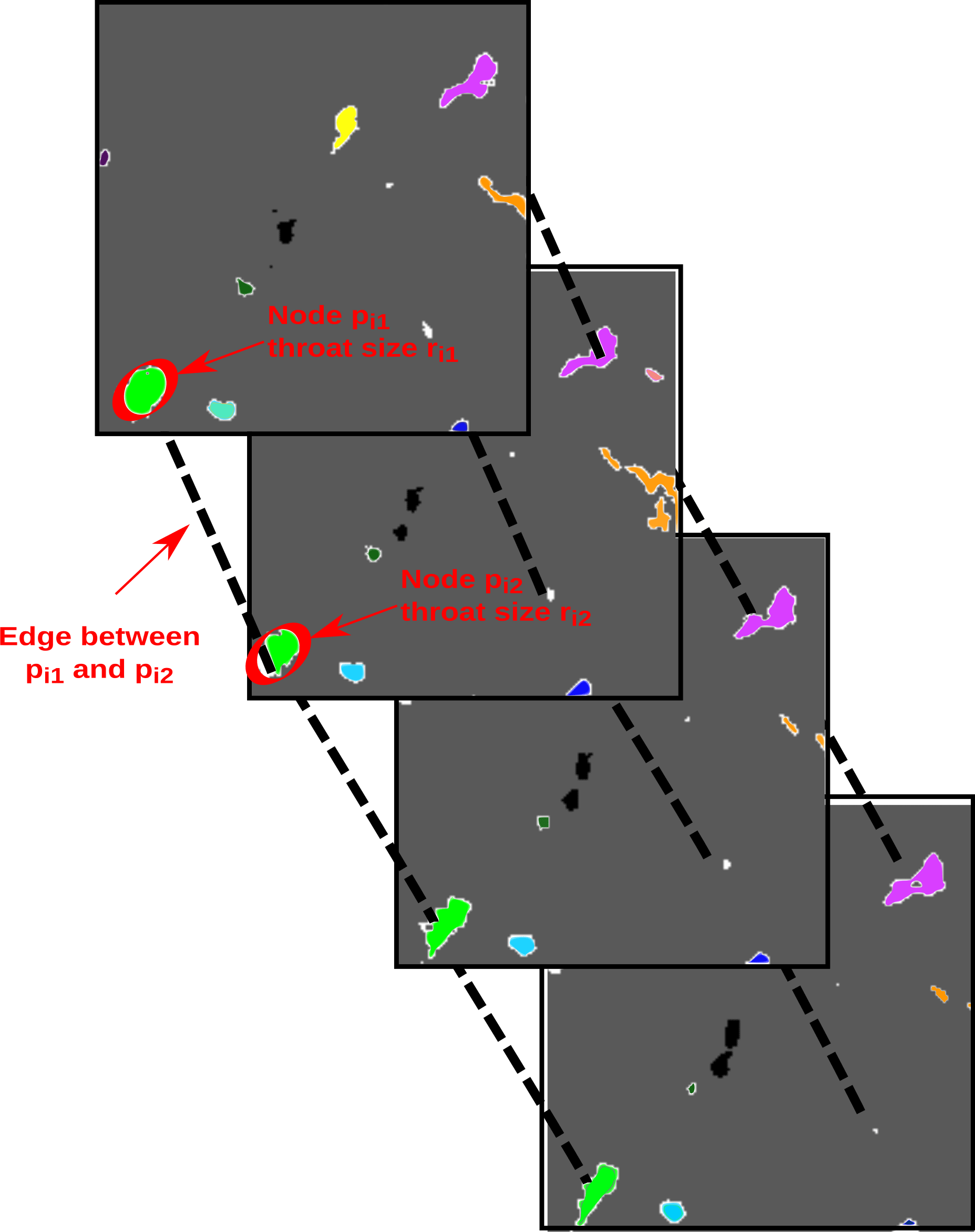
Figure 1Sketch illustrating how the brine channel network is defined. Four horizontal two-dimensional slices are shown with lines connecting adjacent nodes (not all lines are drawn). Different colors represent different brine channels in this sample.
With the definition of the network in place, we next introduce terminology which helps describe the evolution of a brine channel as it progresses downwards through an ice sample. For a fixed node pi, if the intersections in the second part of the definition of an edge above are empty for all other nodes, we say that node has died moving from slice to slice . If there is only one non-empty intersection, we say the node remains. Alternatively, if there are multiple non-empty intersections, we say pi splits. Last, if more than one node at height z overlaps with a single node at height z−1, we say that those nodes join. This terminology allows us to depict the vertical connectivity of the brine phase. Our definition precludes horizontal connectivity as the horizontal extent of a brine region is captured in the definition of the associated node. Since brine channels are primarily vertically oriented with branches splitting both upwards and downwards, this network definition yields a good model for depicting brine movement through the sample.
With this mathematical description of the brine structure, we can calculate statistics about its evolution. For a fixed throat size, r, we compute the probabilities of a node of this size remaining, dying, splitting, or joining. The probability of a node of throat size r remaining in the next step but changing to throat size s is the number of connections divided by the number of nodes of throat size r:
For our discussions in this paper, we aggregate these fine statistics into a single statistic recording the probability that a node of throat size r remains in the next level:
Similarly, we can calculate the probabilities that nodes of size r die, split, or join. Taken together, these probability distributions summarize the evolution of the brine channels in the ice sample statistically.
In summary, the set of probabilities defines a discrete-time probabilistic process. Given a node at a particular height z and throat size r, we know the possible outcomes for this node at height z−1 – remaining, dying, splitting, or joining – and the chance that they occur by looking at the approximations of the probabilities of their occurrence. In other words, taking the collection of {pi,ri} as states and the probabilities as transition probabilities, we have defined a Markov chain modeling the evolution of brine channels within the sample.
We first used standard morphological metrics as defined in previous work to describe the brine network shape and size (Lieb-Lappen et al., 2017). Figure 2 shows the brine volume fraction, definition, and shape of the brine phase for the Butter Point and the Iceberg Site ice cores. The trends in the top half of the core are similar to what we expect since the temperature in the top half of the core is relatively cold and the expected brine volume fraction is small. However, at around 100–120 cm the brine volume fraction begins to increase and the expected C-shape profile begins to appear. Although this trend persists for a few samples, it does not continue as we would expect into the bottom of the core for the warmest temperature samples. This suggests that perhaps the Peltier cooling stage was not warming the temperatures of those samples above approximately −7 ∘C. Since the average temperature of the cold room housing the μCT scanner was −8 ∘C, either the cooling stage warming mode was not functional or was overcome by the ambient temperature. This may highlight that the cooling stage is not sufficiently warming the ice, but instead producing a slush in the pore space that has X-ray attenuating properties between ice and brine. Segmenting all the slush with the brine phase (assuming it is possible to isolate only the slush from signal noise) leads to an overestimate of the brine phase and an inaccurate depiction of brine channel size and connectivity. Conversely, segmenting the slush with the ice phase leads to an underestimate of the brine phase and also an inaccurate depiction of the brine channels. We used segmentation thresholds that split the difference with a threshold halfway between the peak of the brine phase and the peak of the ice phase, recognizing that there was indeed error in segmentation for these warmer samples. Thus, we will treat data points at depths below roughly 120 cm with caution. Unfortunately, this encompasses the region where the brine volume fraction crosses the 5 % critical threshold, limiting our ability to examine the “Rule of Fives” in this paper.

Figure 2Definition and shape of brine channels scanned with a μCT scanner and a Peltier cooling stage set at in situ temperatures. The red squares and blue circles represent ice cores from Butter Point and the Iceberg Site, respectively.
Since the cooling stage did not significantly warm samples beyond −7 ∘C, we were not surprised that general trends shown in Fig. 2 for all metrics did not differ significantly from the same samples scanned isothermally and presented in Lieb-Lappen et al. (2017) as the percolation threshold was not crossed. As in Lieb-Lappen et al. (2017), we used the structure model index (SMI , where S′ is the derivative of the change in surface area after a one pixel dilation, V is the initial volume, and S2 is the initial surface area) to quantify the similarity of the brine phase to plates, rods, or spheres. To quantify size, we calculated a structure thickness by first identifying the medial axes of all brine structures and then fit the largest possible sphere at all points along said axes. The structure thickness is defined as the mean diameter of all spheres over the entire volume. The structure separation is the inverse metric, providing a measurement on the spacing between individual objects. We then calculated the degree of anisotropy by finding the mean intercept length for a large number of line directions, and forming an ellipsoid with boundaries defined by these lengths. The eigenvalues for the matrix defining this ellipsoid are calculated, and correspond to the lengths of the semi-major and semi-minor axes. The ratio of the largest to smallest eigenvalues then provides a metric for the degree of anisotropy, with zero representing a perfectly isotropic object and one representing a completely anisotropic object. We observed that the brine phase specific surface area increased with depth, structure model index was roughly three (indicative of cylindrical objects), structure thickness decreased, structure separation increased, and the degree of anisotropy increased throughout the middle of the core (Fig. 2). From the metrics above, we conclude that brine channels are primarily cylindrical in shape with more branches at lower depths, consistent with previous observations (Lieb-Lappen et al., 2017).
We compared the μCT-measured brine volume fraction to expected values derived from the Frankenstein and Garner relationship relating temperature, salinity, and brine volume fraction (Cox and Weeks, 1983; Frankenstein and Garner, 1967) in Fig. 3. For this analysis, we used the core temperatures measured in the field and salinity values estimated from ion chromatography measured chloride concentrations presented in Lieb-Lappen and Obbard (2015). From 0 to 120 cm, the measured brine volume fractions match the expected values remarkably well. However, below a depth of 120 cm in both cores, the expected brine volume fraction is greater than that measured using μCT. For example, at a depth of 160 cm the expected brine volume fraction is 4.5 and 4.2 times greater than the values measured for samples from the Butter Point and the Iceberg Site ice cores, respectively. This provides an estimate for the degree by which the cooling stage failed to heat the warmer samples in the μCT.
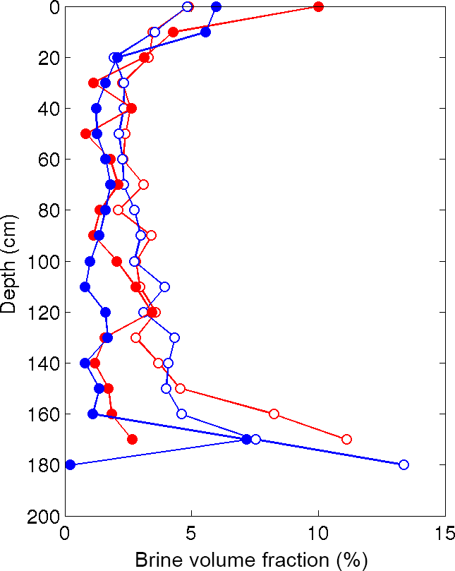
Figure 3Comparing μCT-measured brine volume fraction to the expected values derived from the Frankenstein and Garner relationship (Cox and Weeks, 1983; Frankenstein and Garner, 1967). Results from the Butter Point (red) and the Iceberg Site (blue) cores, where the μCT-measured values are the filled circles and the expected values are the open circles.

Figure 4Average throat size for the five largest brine channels of each sample for the Butter Point ice core. For each channel, at a given depth we calculated the average throat size of all nodes and color-coded accordingly. Note that there are only six channels that connect the top to the bottom of the sample (at depths of 0, 10, 70, and 120 cm).

Figure 5Average throat size for the five largest brine channels of each sample for the Iceberg Site ice core. For each channel, at a given depth we calculated the average throat size of all nodes and color-coded accordingly. Note that there are only six channels that connect the top to the bottom of the sample (at depths of 0, 10, 30, 50, and 170 cm).
4.1 Model definitions
From the binarized images of the brine phase for the Butter Point and the Iceberg Site ice cores, we created a mathematical network. We will use the term network to refer to the entire brine phase of a given sample and/or the entire brine phase of all samples in a given core. For a given sample, we define each brine channel to be a single connected region in the brine network. The number of brine channels per sample ranged from 830 to 4800, with maximum numbers occurring in samples from the top and bottom of the cores. Previous work showed that these brine channels often appear in layers or sheets spaced approximately 0.5–1.0 mm apart due to the ice growth mechanism and original skeletal structure (Weeks and Ackley, 1982). A single brine channel is a complex web containing many different parts, which we will call the branches of the brine channel. As defined previously, a join point is the node where two branches come together and a split point is the node where a single branch splits into multiple branches. We note that flipping the perspective of movement from downwards to upwards changes a split point into a join point and vice versa. This is an important observation since we did not record the vertical orientation of the samples during cutting. Using this terminology, we use techniques from network theory to topologically characterize the brine network, gaining further insight into the connectivity and implications for permeability.
In the analysis below, we use several metrics to describe the topology of the brine network that have important fluid flow implications. We first look at the throat sizes of the brine channels to gain an insight into the quantity of fluid that can move through different regions of a given brine channel. We then look at specific branches, both in terms of the number of branches and the size of each branch to learn more about the specific pathways available for fluid movement. As part of this analysis, we incorporate our various transition probabilities to understand how the likelihood of a given branch to split into multiple branches depends upon the throat size of the parent branch. Finally, we will examine the size distribution of particular paths, looking for “pinch points” that may restrict flow and large regions that can provide maximum flow through the network. Together, these metrics will provide a detailed description of the micro-scale complexity of the brine network.
4.2 Throat sizes of channels and branches
For each brine channel we calculated the average throat size for all nodes {pi} at a given depth in the sample. Figures 4 and 5 show the collection of these throat sizes for the five largest (by vertical extent) brine channels at each depth for the Butter Point and the Iceberg Site cores, respectively. We note that since the entire length of the cores were not scanned, there is no correlation between the five brine channels selected from one sample (e.g., 20 cm depth) to the next (e.g., 30 cm depth). There were six brine channels in each core that connected from the top to the bottom of their respective sample, with the majority of these channels found in samples from the top of each core. Generally speaking, the lengths of the vertical extent of the longest channel decreased with depth from the top of each core to around 60 cm, increased from 60 cm to roughly 120 cm, and then decreased from 120 cm to the bottom of the core. The trend between the top of the core and roughly 120 cm is consistent with what we would expect due to brine volume fraction, temperature, and the expected C-shape profile. The channels from the lower depths, which had even warmer temperatures, did not reach in situ temperatures during scanning as described previously. We also note that both the lengths of the vertical extent and average throat size quickly diminished for channels beyond the few largest ones, as can be seen in the bottom panel of Figs. 4 and 5. Thus, we learn that fluid flow is most controlled by the behavior of the largest brine channel for a given section of sea ice.
The number of branches for a particular brine channel has potentially significant implications for fluid flow and permeability, such as influencing the rate at which chemical species may pass through the sea ice (Newman, 2011; Santiago et al., 2014; Yang et al., 1995). By increasing the number of branches, split points can increase the number of potential paths through the sample. A higher number of paths increases the probability of finding a path connecting the top and bottom of a sample, thereby crossing the percolation threshold (Sahimi, 2011). Alternatively, split points can represent bottle-necks if the resulting child branches have smaller throat sizes than the parent throat, measured either as a minimum or as an aggregate. We observed that the largest channel in a cubic sample had by far the largest number of branches, with the quantity dependent upon the ice type. For example, in a columnar ice sample (70 cm depth of the Butter Point ice core) the largest channel had a maximum of 20 branches at a given depth within the sample. For comparison, the maximum number of branches for a sample in the frazil ice region at the top of the core was 124 nodes at a single depth. As expected, we find that brine channels in frazil ice have many more branches than brine channels in columnar ice, providing more distinct pathways for brine to move through the sample.
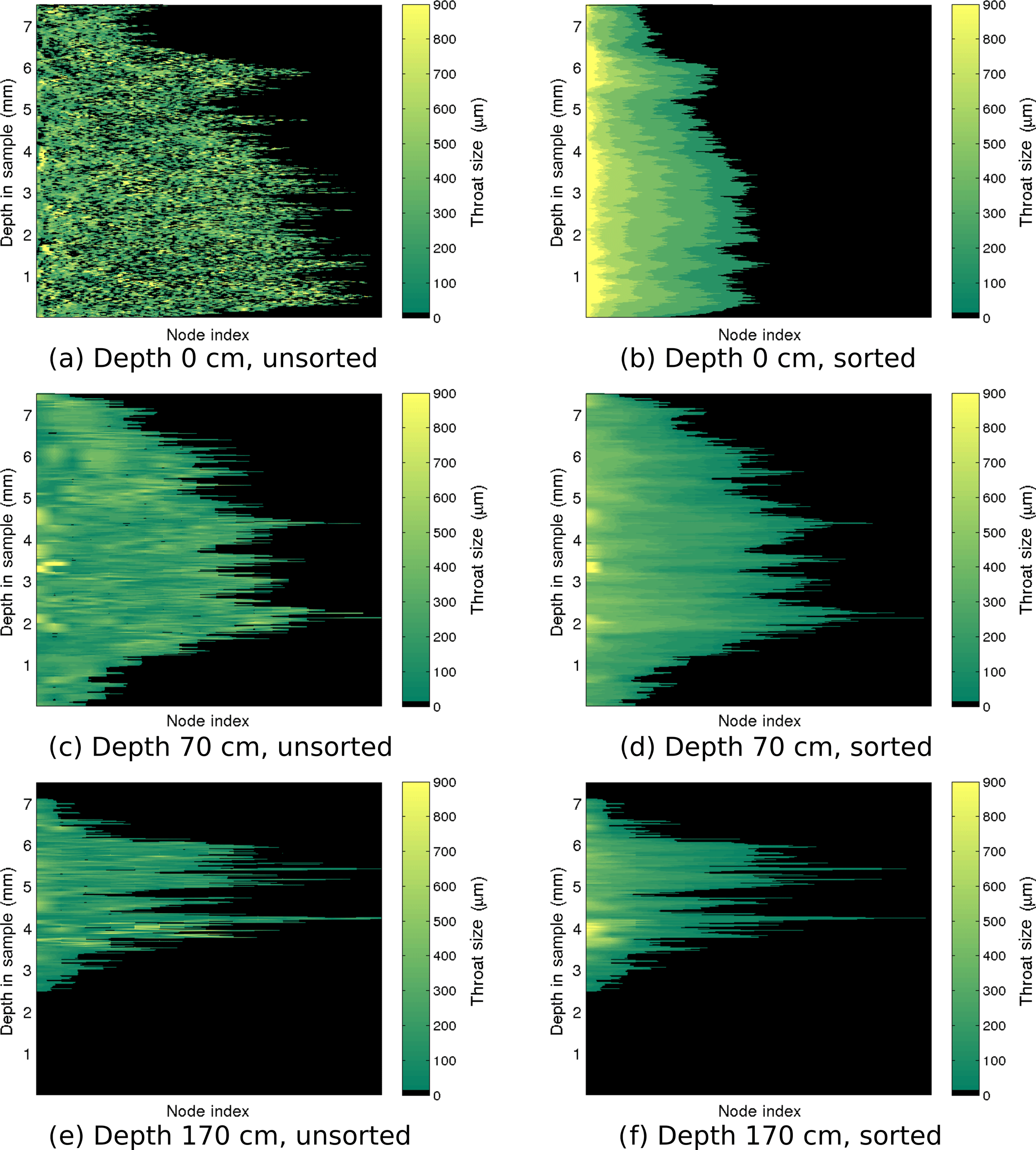
Figure 6Throat size ri of each node for the largest channel of representative samples in the Butter Point core. The top, middle, and bottom rows show the largest brine channel from the sample at 0, 70, and 170 cm, respectively. The left panels show the throat sizes at each depth in the sample with nodes sorted by location, not by size. The right panel sorts the nodes by throat size in descending order.
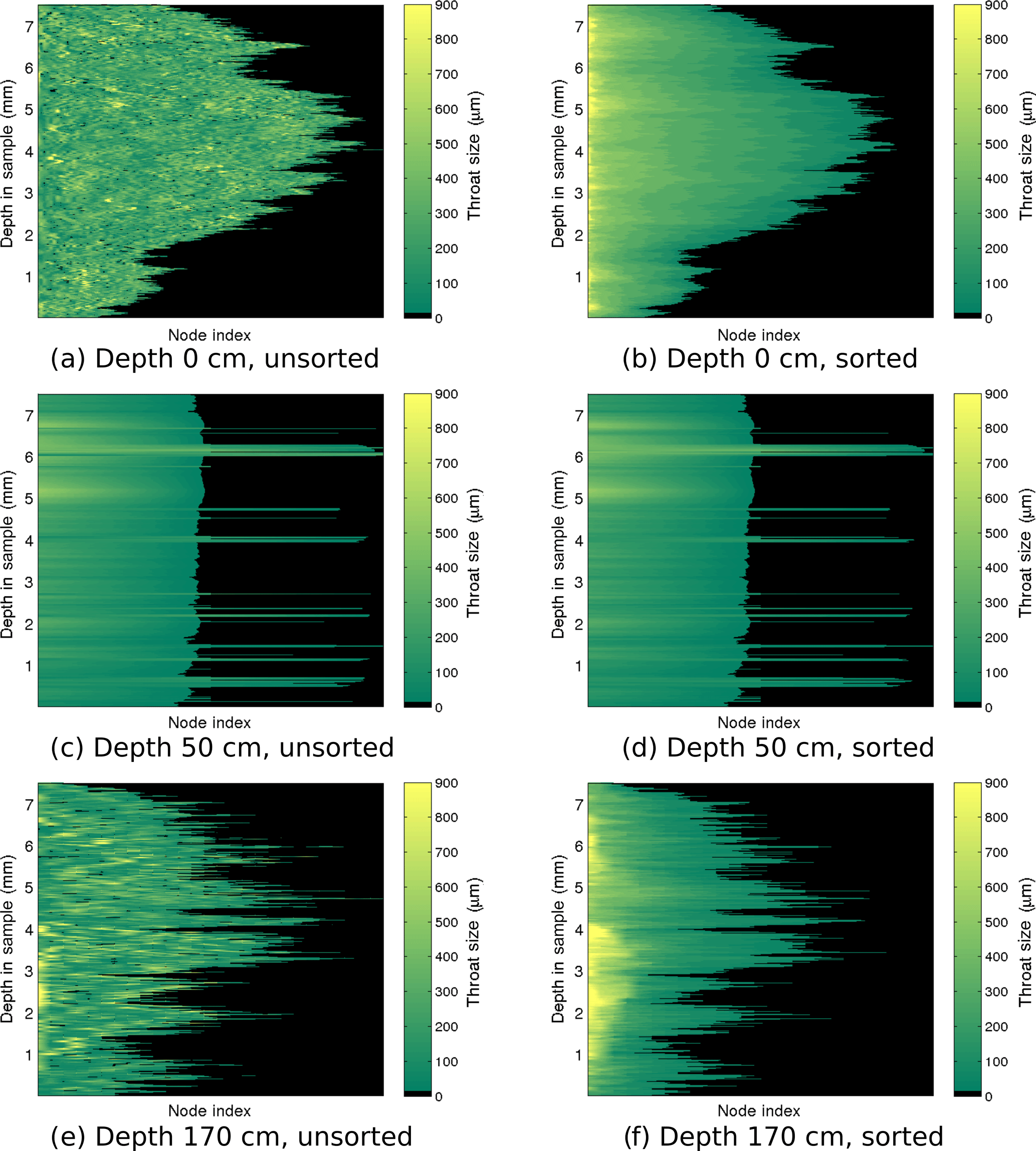
Figure 7Throat size ri of each node for the largest channel of representative samples in the Iceberg Site core. The top, middle, and bottom rows show the largest brine channel from the sample at 0, 50, and 170 cm, respectively. The left panels show the throat sizes at each depth in the sample with nodes sorted by location, not by size. The right panel sorts the nodes by throat size in descending order.

Figure 8The figure shows {ri} probability distributions showing the likelihood a node dies, remains, splits, or joins as a function of the throat size r. The top four figures show probability distributions for frazil ice while the bottom four figures show probability distributions for columnar ice. Note that to complete these figures, in addition to the Butter Point and the Iceberg Site cores, we used two additional first year sea ice cores from previous work (Lieb-Lappen et al., 2017). Butter Point is shown in black, the Iceberg Site is shown in blue, and the two additional first year ice cores are shown in red and black.
To gain insight into the behavior of a channel, we visualized the number of branches and distribution of throat sizes by plotting the throat size ri of each node pi for the largest brine channel. Figures 6 and 7 show the throat sizes as a function of depth in the sample for three different representative sample depths: top, middle, and bottom of the Butter Point and the Iceberg Site cores, respectively. For each channel shown, there is a plot of {ri} at each depth sorted by physical location in a two-dimensional grid (working line by line), not by size. A second corresponding plot shows node sizes sorted by descending {ri} for a given depth in the channel. The first set of plots illustrate the connectivity of given branches, while the second set provide a visualization of the distribution of ri. The sample taken from the top of each core is from a region of frazil ice, which we would expect to have brine channels that are not well connected and have a distribution of throat sizes independent of depth in the sample. In both Figs. 6 and 7, panel (a) confirms this while panel (b) shows that there was an even distribution of throat sizes. The two plots for mid-depth networks (70 cm) are quite similar, illustrating less tortuosity and easier ability to track particular branches in the brine channel. The bottom sample of the Iceberg Site core had much larger throat sizes, although this sample was an anomaly in Fig. 2. We did not observe a direct correlation between the number of branches and the throat size of those branches, as the distribution of throat sizes appeared to be more dependent upon the particular depth of the sample in the ice core, and consequently, the ice type of that sample. From this analysis, we learn that although there may be more branches for a given brine channel in frazil ice, the branches have better vertical connectivity in columnar ice. This means that fluid can more readily move upwards or downwards through the larger well-connected brine channels in columnar ice.
4.3 Probability distribution of branching nodes
Next we examined the branching of particular nodes to understand the behavior of particular fluid flow paths. Following a branch of a channel downwards, at an individual node the branch may end, continue onwards, or split into multiple branches. Conversely, by looking upwards, a node can be considered to be the first in a new branch, the continuation of a branch, or the joining point of multiple branches. Thus, for each node in a brine channel, we can count the number of edges above (incoming) and below (outgoing) to determine the degree of splitting or joining of branches in the channel (Newman, 2011). The large majority of nodes do not display branching, and the number of two-way splits/joins was roughly the same as the number of times a branch started/ended. We observed decay in frequency with increasing quantity of splits/joins. The Iceberg Site core had a larger number of higher order branching with a significant number of seven-way or eight-way splits/joins. A branch that splits is most likely to split into only two child branches, and thus for example, a contaminant introduced at a point source is likely restricted to a small horizontal region, following only a few separate paths through the ice. When a split occurred, we compared ri for the parent node to the collection of ri for the children nodes with similar behavior observed in both cores. 84 % of the time for the Butter Point core and 86 % of the time for the Iceberg Site, the sum of the throat sizes for the children node were greater than that of the parent node. However, the parent node was still larger than the largest child node 67 % of the time for the Butter Point core and 68 % of the time for the Iceberg Site core. Thus, we learn that larger brine channels are more likely to split than smaller channels, and after the split, the fluid can access a larger region of the sea ice.
With knowledge of the total number of split points and join points, we then investigated the likelihood that branching was dependent upon the throat size. Figure 8 shows the probability distributions for pockets dying, remaining, joining, and splitting for two regions of each of the four samples, frazil ice and columnar ice. Note that for these plots, we used two additional first-year sea ice cores from previous work in addition to the Butter Point and the Iceberg Site cores (Lieb-Lappen et al., 2017). The most basic difference between the two regions is that larger pocket sizes do not appear in columnar ice. However, for ranges of r occurring in both regions, the shapes of the plots are similar. While small pockets can disappear, larger ones generally do not – the probabilities tend to zero (as marked by arrows in the plots in the first column). For pockets that remain but do not split or join with others, smaller pockets remain with lower probability (because more of them vanish) but then the probabilities follow an inverted parabolic trajectory, peaking around r=130 µm. An interesting difference appears as throat size grows. In columnar ice, for throat size around r=500 µm, we see two distinct behaviors. Some sizes remain with probability one (indicated by the top arrow in the second plot of the second row), while others remain with probability zero (bottom arrow). For the latter, looking at the last plot in the bottom row, we see these pockets are splitting into two or more pockets (indicated by the top arrow in that plot). This gives a signature for columnar ice – most brine channels simply continue on with slightly varying throat size but the ones that change generally split, creating a fork in the channel.
In frazil ice, the story for pockets that vanish is the same, as throat sizes become larger, they do not vanish in the next level. For remaining, splitting, and joining, however, there are new wrinkles in frazil ice relative to columnar ice. For pockets that remain, for larger throat sizes we see three types of behavior, two of which are similar to the behaviors in columnar ice (indicated by the top and bottom arrows of the second plot in the first row); however, a third behavior, where fifty percent of pockets remain, is new for frazil ice (middle arrow). This new behavior is echoed in the probabilities of splitting and joining (indicated by the middle arrows in those plots) which shows that in this regime, brine channels have a complex behavior, remaining, splitting, and joining with high frequency. This third category of behavior for large throat sizes is a signature of frazil ice.
In addition, we summed the total number of edges leaving (splits) and entering (joins) each node over all nodes for the five largest brine channels of each sample. Figure 9 plots these raw counts and the difference between the two are given for the Butter Point and the Iceberg Site cores. When we consider split points and join points separately, we are considering the network as a graph with directed edges. The difference between the number of splits and joins (i.e., difference between number of incoming and outgoing edges) is a metric for the topological complexity of a network. The raw counts for number of splits and joins had roughly C-shape profiles for both cores, with largest values and variability observed towards the bottom of the core. This is to be expected because the warmer part of the core allows for greater interconnectivity of branches in the brine network. For all brine channels, the number of splits was quite similar to the number of joins, and hence the differences between the two were quite small. However, there was still a general C-shape profile between 0 and 140 cm, indicating that topological complexity is greatest near the top and bottom of the core. This is consistent with frazil ice in the top of the core and increased branching in the warmer ice. Interestingly, both cores showed a decrease in topological complexity for the lowest samples below 140 cm. This could either be an artifact of not achieving actual in situ temperatures with the cooling stage, or potentially an indication of a thought-provoking trend. If samples were not reaching in situ temperatures, isolated channels may not have rejoined upon warming from storage temperatures, thereby reducing the number of split points and join points. Alternatively, a possible explanation of a real trend could be that as brine channels widen for the warmest samples, branches join together, reducing the topological complexity. A consequence of reducing the number of branches is a reduction in the number of split points and join points.
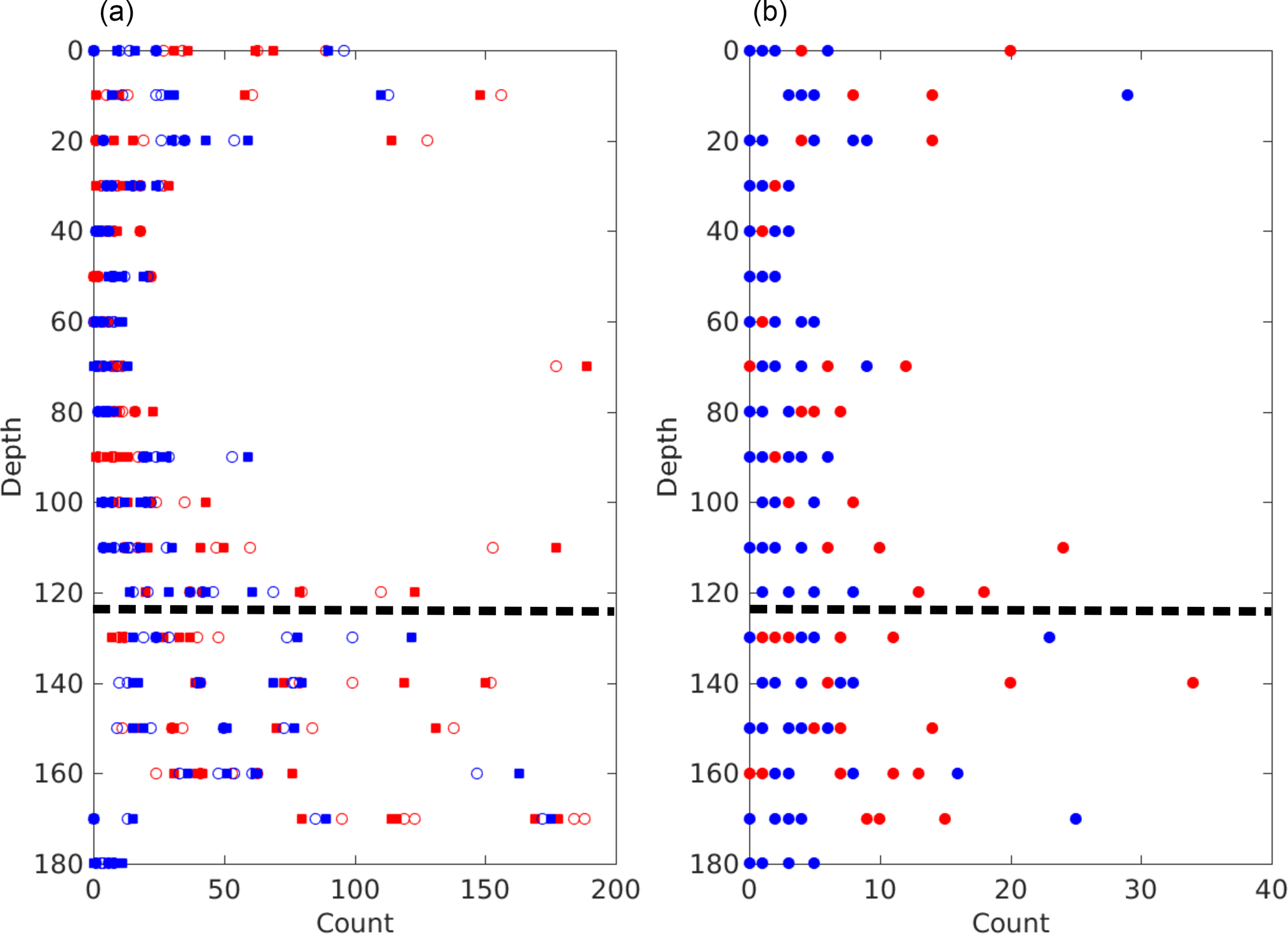
Figure 9Topological complexity of the five largest brine channels in each sample for both the Butter Point (red) and the Iceberg Site (blue) cores. The panel (a) shows the total number of splits (open circles) and joins (filled squares) over all nodes in a given channel. The panel (b) shows the absolute value of the difference between the number of splits and joins. The dashed line highlights the depth below which there is concern regarding the effectiveness of the cooling stage and whether samples were scanned at actual in situ temperatures.

Figure 10Cumulative distribution functions for number of brine channels as functions of the total number of pixels in the channel. The panels (a, b) are for the Butter Point and the Iceberg Site ice cores, respectively. In both panels, each line represents a different sample depth where the lines are colored on a gradient from red representing the top of the core to blue for the bottom of the core. Note that pixels in the original μCT images are 15 µm on each edge. Note that all values for depth are in centimeters.
4.4 Capacity for fluid flow
We next examined the fluid flow capacity of each channel by both summing the number of pixels associated with all nodes for each channel and summing the total throat sizes of all nodes in each channel. We note that this represents a region larger than the pathways used for current fluid flow since many branches do not connect the top of a sample to the bottom. However, when the ice begins to warm and the branches become more interconnected, the process will likely start from the existing regions containing brine. Thus, this metric offers a starting place for comparing the capacity for fluid flow across different samples. Figure 10 shows cumulative distribution functions for the number of brine channels as functions of the total number of pixels in the channel, with each line representing a different sample depth. The lines are colored on a gradient from red representing the top of the core to blue for the bottom of the core. The distribution functions for all depths on both cores were remarkably similar, and pairwise Kolmogorov–Smirnov tests did not detect that any two curves were from different probability distributions (p ≥ 0.1) (Graham and Hogg, 1978; Massey, 1951). Both cores did show a trend of increased probability of brine channels with more pixels occurring at shallower depths, with a more robust trend observed in the Iceberg Site core. This trend could be due to samples at lower depths having an increased number of isolated small channels that have yet to connect to larger channels. Since there is doubt as to whether the samples below 120 cm were scanned at their in situ temperatures, perhaps these small isolated channels would have connected to larger channels under warmer conditions. Figure 11 presents similar cumulative distribution functions for the number of brine channels as functions of the summed throat size of all nodes in the channel. The curves yield the same observations as before, with the Iceberg Site core again having a stronger correlation of increased probability of larger channels occurring at shallower depths. Likewise, Kolmogorov–Smirnov tests did not detect any two curves representing different probability distributions (p ≥ 0.1). Any noticeable changes to the relative shape of the curves represent disproportionate changes in the shape of the brine channel with size of the channel, however, these variations were quite minor. In general, the shape of the curves in Fig. 11 are similar to those in Fig. 10. Thus, we conclude that brine channels in samples near the top of the core provide fluid with multiple distinct pathways to move through the sample, while deeper in the core there are only a few large channels with many small isolated paths that may connect under warmer ice conditions.
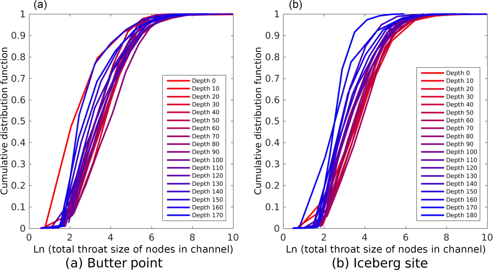
Figure 11Cumulative distribution functions for number of brine channels as functions of the summed throat size of all nodes in the channel. The panels (a, b) are for the Butter Point and the Iceberg Site ice cores, respectively. In both panels, each line represents a different sample depth where the lines are colored on a gradient from red representing the top of the core to blue for the bottom of the core. Note that throat sizes in the original μCT images are 15 µm on each edge. Note that all values for depth are in centimeters.
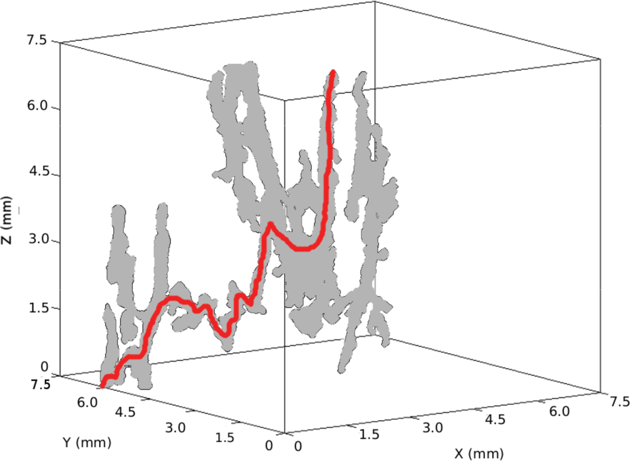
Figure 12Largest brine channel at 70 cm in the Butter Point ice core. Although this brine channel connects from top to bottom, there is not a directed path that does so. Any connecting path involves movements both upwards and downwards. One such path is highlighted in red.

Figure 13Probability distributions of paths connecting the top to the bottom for all brine channels in the Butter Point ice core. Only paths greater than 50 steps, or 750 µm were considered. Left, middle, and right panels represent channels where rf<1500 µm, µm, and rf ≥ 52 500 µm, respectively. Top, middle, and bottom rows represent probability distributions for rmin, rmax, and summed throat size, respectively. For all panels, the colors red, blue, and green represent channels where r1<1500 µm, µm, and r1≥52 500 µm, respectively.
4.5 Following individual fluid flow paths
To further assess fluid flow capabilities, we analyzed individual branches of brine channels to isolate particular paths through the network. By construction, moving from pi to pj along an edge must either increase or decrease the height in the sample by one step (15 µm). First, we allowed only downward flow along the edges, considering paths starting from the first node. Since the network does not allow lateral movement, each step along an edge corresponds to a 15 µm step downwards. Although previously six brine channels were found that connected the top to the bottom of a given sample, no such paths were found in the directed graphs. This is because all paths connecting the top to the bottom of a sample required some movement upwards along a branch in order to reach the bottom. Figure 12 shows an example of a brine channel where although the network is connected, any connecting path involves both upward and downward flow, such as the path highlighted in red. Thus, we selected the longest downward directed path from each brine channel, as well as any additional paths of the same length. This mimics a natural process such as gravity drainage, allowing us to study its influence on brine movement in the absence of pressure forces that aid upwards transport. Summing over all brine channels in the Butter Point core resulted in 63 763 directed paths, of which 15 316 paths had a length of at least 50 steps (750 µm). We then used this smaller subset for statistical analysis of minimum throat size (rmin), maximum throat size (rmax), and summed throat size. Future work will use this model to statistically recreate brine channels that have this same distribution of brine channel sizes.
We completed a similar analysis on the brine channel network, however this time allowing for both upward and downward flow. Allowing for upward flow can present a challenge in tracking various pathways if there is a repeating loop. Thus, we only considered paths that reached every node but had no loops. In the language of networks, we avoided complexities arising from cycles by only considering different spanning trees. We used a depth-first search algorithm to find all paths reaching the maximum vertical extent of each channel (Newman, 2011; West, 2001). We checked results through comparison of the distance obtained using Dijkstra's algorithm for finding the shortest-path tree (Dijkstra, 1959; West, 2001). This resulted in 36 449 paths over all the brine channels in the Butter Point core, of which 1753 were of length 50 steps (750 µm). We note that we can use the adjacency matrix to calculate the number of different walks (paths including cycles) that connected the top and bottom of a sample (West, 2001). However, due to the size of the adjacency matrix, this became computationally too expensive for large brine channels.
We used the 1753 paths of length greater than 50 steps to develop probability distributions for basic network statistics important for fluid flow such as rmin, rmax, and summed throat size of the path. These statistics can yield valuable information regarding the location and distribution of “pinch points,” large channels, and total fluid flow through a brine channel. First, the paths were split into three categories based upon the ending node (pf) throat size: rf<1500 µm, µm, and rf≥52 500 µm. Then, we split each category into three groups based upon the throat size of the starting node (p1), using bins of the same size (r1<1500 µm, µm, and r1≥52 500 µm). This division resulted in splitting the paths into nine separate sub-categories. For each sub-category, we calculated the probability distributions for rmin, rmax, and summed throat size of the path and we present these histograms in Fig. 13. All plots are color-coded by r1, with red, blue, and green histograms representing small, medium, and large throats, respectively. All histograms show the similar trend that both r1 and rf have a strong influence on resulting metrics, with larger r1 and/or rf having larger rmin, rmax, and total volumes. The magnitude of rf had slightly more of an impact, particularly on rmin. There were no clear general trends in regards to the shape of the distributions. However, we note that for the smallest rf, all three histograms for rmin had a large peak around 30 µm (Fig. 13, top row). This peak corresponds to the smallest measurable branches, and we could potentially remove these paths from current fluid flow analysis. However, as the ice begins to warm, these “pinch points” are likely to have a significant impact on crossing percolation thresholds.
The primary objective of this work has been to improve our characterization of brine channel topology, morphology, and connectivity, in order to provide sea ice modelers with a greater level of detail on the factors that affect microstructural transport properties. While most percolation models use coarse microstructural properties to form a statistical basis for predicting connectivity, ours derives finer-grained statistics empirically, allowing for better representation of the range of physical properties found in sea ice of different types and conditions. We can statistically model the evolution of brine channels as we move downwards through the sea ice cover. Beginning with an initial brine pocket, our estimates of the evolution probability distributions from μCT scans of sea ice samples tell us how the channel changes as we progress downward through the sample – Does it grow? Shrink? Split into more than one branch? Join up with more than one branch? Close off entirely?
Overall, we observed similar morphological profiles for both first-year sea ice cores. Topological complexity had the expected C-shape profile that is consistent with complex frazil ice in the top of the core, relatively cold columnar ice below it, and increasingly warmer columnar ice at lower depths. However, we did not have good success in imaging and thresholding ice with the warmest in situ temperatures at the bottom of the core.
Our estimates of the evolution probability distributions provides a stochastic model of brine channels within sea ice at different temperatures, extending the percolation models described above. Their structural features reveal the onset of transitions between different types of ice: in our analysis, we see different statistical features that delineate frazil and columnar ice. Further, the level of detail inherent to this technique allows us to quantify some of the finer details of brine channel structure and development. In addition to estimating the expected brine volume and permeability for ice at a fixed temperature, we can see when and why permeability arises by analyzing the probabilistic structures. For example, Fig. 8 shows a stark structural difference between frazil and columnar ice which points to the onset of percolation: brine pockets in frazil ice larger than about 1 mm are extremely likely to join or split while the largest brine pockets in columnar ice are more likely to persist. We observe that brine channels in columnar ice simply continue downwards with little change in size. For those in which there is a significant change in size, there is a likely fork leading to a split in the channel. A higher probability of interconnections between brine channels translate directly into a higher probability of permeability of the ice.
When examining the branching in brine channels, we observe that the largest channels have the greatest number of branches, but overall brine channel size does not appear to have a direct correlation with the number of branches. Brine channel size is most dependent upon the depth and consequently ice type. When a split in a brine channel does occur, it is most likely to split into two child branches, and after the split, the brine generally has access to a larger region of the sea ice than before. Starting and ending brine pocket sizes are strongly correlated with the flow capacity with larger initial/final sizes strongly indicative of increased flow. We detected pinch points in the brine channels that are critical points when determining whether the sea ice cover has crossed the percolation threshold. However, further work is needed in examining warmer ice with greater brine volume fractions.
Our framework enables us to statistically replicate the pore structure of sea ice at different depths and temperatures. The next step for this work is to create a brine channel network from the probability distributions presented here. For a sample at a given depth/temperature, first an initial region at the top of the ice would be selected with size consistent with the statistics shown here. The brine channel could grow or shrink, split into multiple branches, join with other branches, remain constant, or stop, all with probabilities dependent upon the thickness, depth/temperature, and proximity to other brine channels. The model described herein can help address questions such as how microstructural changes may be path dependent (e.g., whether to consider both upwards and downwards flow), how fluid flow may vary with depth, and what are the percolation implications of temperature fluctuations in an ice core. In summary, we successfully developed a method using μCT imaging to characterize the geometry of brine channels, whereby we can parameterize the pore networks using topological techniques that can be adjusted for depth and temperature, correlated with physical properties, and used in dynamical models of sea ice.
All data for this paper are archived with the U.S. Antarctic Program Data Center (USAP-DC) under the DOI https://doi.org/10.15784/600158.
The authors declare that they have no conflict of interest
This research was supported by US National Science Foundation (NSF) grant
PLR-1304134. The views and conclusions contained herein are those of the
authors and should not be interpreted as representing official policies,
either expressed or implied, of the NSF or the United States Government.
Edited by: Jennifer Hutchings
Reviewed by: Christian Sampson and Malcolm Ingham
Berkowitz, B. and Balberg, I.: Percolation Approach to the Problem of Hydraulic Conductivity in Porous Media, Transport Porous Med., 9, 275–286, 1992. a
Cox, G. F. N. and Weeks, W. F.: Brine Drainage and Initial Salt Entrapment in Sodium Chloride Ice, Tech. Rep. Research Report 345, CRREL, Hanover, NH, 1975. a
Cox, G. F. N. and Weeks, W. F.: Equations for Determining the Gas and Brine Volumes In Sea-Ice Samples, J. Glaciol., 29, 306–316, 1983. a, b
Delerue, J. F., Perrier, E., Timmerman, A., and Swennen, R.: 3D Soil Image Characterization Applied to Hydraulic Properties Computation, in: Applications of X-ray Computed Tomography in the Geosciences, edited by: Mees, F., Swennen, R., Van Geet, M., and Jacobs, P., Geological Society Special Publications, London, 215, 167–175, 2003. a
Dijkstra, E. W.: A Note on Two Problems in Connexion with Graphs, Numerische Mathematik, 1, 269–271, 1959. a
Dong, H., Fjeldstad, S., Alberts, L., Roth, S., Bakke, S., and Øren, P.-E.: Pore Network Modelling on Carbonate: A Comparative Study of Different Micro-CT Network Extraction Methods, in: Soc. Core Anal. Int. Symp., UAE, Abu Dhabi, UAE, 29 October–2 November 2008. a
Dwyer, R. A.: Maximal and Minimal Balls, Comp. Geom.-Theor Appl., 3, 261–275, 1993. a, b
Fatt, I.: The Network Model of Porous Media, Petroleum Transactions, AIME, 207, 144–181, 1956. a
Frankenstein, G. and Garner, R.: Equations for Determining the Brine Volume of Sea Ice from −0.5∘ to −22.9 ∘C, J. Glaciol., 6, 943–944, 1967. a, b
Freitag, J.: Untersuchungen zur Hydrologie des arktischen Meereises – Konsequenzen für den kleinskaligen Stofftransport, Ber. Polarforsch/Rep. Pol. Res., 1–150, 1999. a
Golden, K. M.: Percolation Models for Porous Media, in: Homogenization and Porous Media, edited by Hornung, U., Springer-Verlag, Berlin, Germany, 27–43, 1997. a
Golden, K. M., Ackley, S. F., and Lytle, V. I.: The Percolation Phase Transition in Sea Ice, Science, 282, 2238–2241, 1998. a, b, c, d
Golden, K. M., Eicken, H., Heaton, A. L., Miner, J., Pringle, D. J., and Zhu, J.: Thermal Evolution of Permeability and Microstructure in Sea Ice, Geophys. Res. Lett., 34, L16501, https://doi.org/10.1029/2007GL030447, 2007. a
Graham, J. E. and Hogg, R. V.: Studies in Statistics, Mathematical Association of America, Washington DC, 1978. a
Heijmans, H. J. A. M. and Roerdink, J. B. T. M.: Mathematical Morphology and its Applications to Image and Signal Processing, Kluwer Academic Publishers, Dordrecht, Netherlands, 1998. a
Lieb-Lappen, R. M. and Obbard, R. W.: The role of blowing snow in the activation of bromine over first-year Antarctic sea ice, Atmos. Chem. Phys., 15, 7537–7545, https://doi.org/10.5194/acp-15-7537-2015, 2015. a
Lieb-Lappen, R. M., Golden, E. J., and Obbard, R. W.: Metrics for interpreting the microstructure of sea ice using X-ray micro-computed tomography, Cold Reg. Sci. Technol., 138, 24–35, https://doi.org/10.1016/j.coldregions.2017.03.001, 2017. a, b, c, d, e, f, g
Massey, F. J.: The Kolmogorov-Smirnov Test for Goodenss of Fit, J. Am. Stat. Assoc., 46, 68–78, 1951. a
Nakawo, M. and Sinha, N. K.: A Note on Brine Layer Spacing of First-Year Sea Ice, Atmos. Ocean, 22, 193–206, 1984. a
Newman, M. E. J.: Networks: An Introduction, Oxford University Press, New York, 2011. a, b, c, d
Obbard, R. W., Lieb-Lappen, R. M., Nordick, K. V., Golden, E. J., Leonard, J. R., Lanzirotti, A., and Newville, M. G.: Synchrotron X-ray Fluorescence Spectroscopy of Salts in Natural Sea Ice, Earth Space Sci., 3, 463–479, https://doi.org/10.1002/2016EA000172, 2016. a, b
Obbard, R.: Bromide in Snow in the Sea Ice Zone, U.S. Antarctic Program Data Center (USAP-DC), https://doi.org/10.15784/600158, 2016.
Petrich, C., Langhorne, P. J., and Sun, Z. F.: Modelling the Interrelationships Between Permeability, Effective Porosity and Total Porosity in Sea Ice, Cold Reg. Sci. Technol., 44, 131–144, 2006. a, b
Pierret, A., Capowiez, Y., Belzunces, L., and Moran, C. J.: 3D Reconstruction and Quantification of Macropores using X-Ray Computed Tomography and Image Analysis, Geoderma, 106, 247–271, 2002. a
Pringle, D. J., Miner, J. E., Eicken, H., and Golden, K. M.: Pore Space Percolation in Sea Ice Single Crystals, J. Geophys. Res., 114, C12017, https://doi.org/10.1029/2008JC005145, 2009. a, b, c
Sahimi, M.: Flow and Transport in Porous Media and Fractured Rock, Wiley-VCH, Weinheim, Germany, 2011. a
Santiago, E., Velasco-Hernández, J. X., and Romero-Salcedo, M.: A Methodology for the Characterization of Flow Conductivity through the Identification of Communities in Samples of Fractured Rocks, Expert Syst. Appl., 41, 811–820, 2014. a
Silin, D. and Patzek, T.: Pore Space Morphology Analysis using Maximal Inscribed Spheres, Physica A, 371, 336–360, 2006. a, b
Thomas, D. N. and Dieckmann, G. S.: Sea Ice, Wiley-Blackwell, Hoboken, NJ, 2009. a, b
Weeks, W. F. and Ackley, S. F.: The Growth, Structure, and Properties of Sea Ice, Tech. Rep. Monograph 82-1, CRREL, Hanover, NH, 1982. a, b
West, D. B.: Introduction to Graph Theory, Prentice Hall, Upper Saddle River, NJ, 2001. a, b, c
Yang, G., Myer, L. R., Brown, S. R., and Cook, N. G. W.: Microscopic Analysis of Macroscopic Transport Properties of Single Natural Fractures Using Graph Theory Algorithms, Geophys. Res. Lett., 22, 1429–1432, 1995. a
Zhu, J., Jabini, A., Golden, K. M., Eicken, H., and Morris, M.: A Network Model for Fluid Transport through Sea Ice, Ann. Glaciol., 44, 129–133, 2006. a, b