Satellite telemetry of surface ablation to inform spatial melt modelling and event-scale monitoring, Place Glacier, Canada

We designed and deployed four low-cost automated smart stakes equipped with Iridium satellite telemetry to monitor Place Glacier, British Columbia, Canada during the 2024 ablation season. The smart stakes recorded air temperature, relative humidity, and distance to glacier surface every 15 min from 8 May to 14 November  2024. This high-temporal resolution, near real-time melt data sampled an elevation gradient and across varied glacier surfaces. Smart stake data yielded ice melt factors of −4.21 to −4.87 mm w.e. °C⁻¹ d⁻¹ and snow melt factors of −3.52 to −4.08 mm w.e. °C⁻¹ d⁻¹ , consistent with previous studies. Shortwave radiation melt factors were $-\mathrm{0.041}\pm \mathrm{0.006}$ and $-\mathrm{0.029}\pm \mathrm{0.025}$ mm w.e. W⁻¹ m⁻² d⁻¹ for snow and ice, respectively. We combined the melt factors with repeat airborne lidar, daily air temperature lapse rates, incoming shortwave radiation, and satellite snow cover observations in a distributed Enhanced Temperature-Index model for the 2024 ablation season. Validation against manual ablation stakes showed reasonable agreement (R²=0.63, RMSE = 0.33 m w.e.) and improved agreement against geodetic mass change (R²=0.82, RMSE = 0.23 m w.e.). The distributed melt model estimated a total seasonal melt volume of 12.1×10⁶ m³, representing a summer mass balance of −4.33 m w.e. for the glacier. Event-scale analysis revealed that three multi-day heat events with mean daily air temperatures above 10 °C (5–22 July, 1–12 August, and 29 August–9 September) that accounted for over half of the total seasonal melt despite comprising only one-third of the ablation season. Maximum daily melt rates reached −77 mm w.e. d⁻¹ during these heat events. On-glacier air temperature inversions up to +8.0 °C km⁻¹ were observed on multiple occasions, highlighting the importance of distributed temperature measurements for accurate melt modelling. The low-cost smart stake system demonstrates significant potential as a transferable automated glacier monitoring system, providing near real-time data transmission.

1 Introduction

Glacier mass balance is a key metric used to quantify the impact of regional and global climate change (IPCC, 2023). With a warming climate and increases in summer heat waves, the process of ablation – which includes melting and sublimation of snow and ice – is fundamental in determining a glacier's overall health (Cremona et al., 2023; Østrem, 1973; Pelto, 2019; Reyes and Kramer, 2023). Ablation is commonly measured by surveying physical stakes that are drilled into the surface of a glacier (Cogley et al., 2011). While these in-situ measurements are critical to improve mass balance models and understand long-term mass balance trends, glaciers with in-situ records are rare and those records are typically only available at monthly or seasonal time scales (Hugonnet et al., 2021; Moore and Demuth, 2001; Pelto, 2019).

In contrast, airborne and spaceborne remote sensing techniques are used to study mass balance over large areas (Beedle et al., 2014; Clarke et al., 2013; Hugonnet et al., 2021; Johnson et al., 2013; Kääb et al., 2012). Remote sensing can be used to, for example, map glacier extents, track snowline elevations, measure glacier velocities, and quantify volume changes (Bevington and Menounos, 2022, 2025; Hugonnet et al., 2021; Lorrey et al., 2022; Østrem, 1973; Pelto, 2019; Rabatel et al., 2012). While airborne methods often have a higher spatial resolution and vertical accuracy than spaceborne data, these data can be expensive and few areas have repeat airborne lidar surveys over glaciers (Donahue et al., 2023; Menounos et al., 2025; Pelto et al., 2019). Despite their many advantages, remote sensing data have significant limitations that are often mitigated with in-situ observations (Podgórski et al., 2019), for example, the compromise between spatial and temporal resolution of the dataset, geometric distortions and shading issues in steep terrain, and the ongoing challenge of cloud cover in optical imagery. New methods are therefore emerging that increase the temporal resolution of melt observations throughout the ablation season (Cremona et al., 2023; Wickert et al., 2023). The increased temporal resolution facilitates the investigation of event-scale meteorological forcing on ablation and provides enhanced observational melt data for model testing.

Real-time glacier melt data can be used to inform glacier mass balance and hydrological models, which are of particular interest for flood forecasting (Cremona et al., 2023; Wickert et al., 2023). Automatic weather stations (AWS) are one solution to the need for high temporal resolution real-time observations (e.g. Wheler and Flowers, 2011; Wickert et al., 2019). This equipment is generally costly and can be cumbersome to install and maintain on a dynamic glacier surface (e.g. large batteries, large tripods, and challenging to move on foot). Due to the high cost, only one station is typically used in combination with a network of traditional manual ablation stakes (e.g. Bash et al., 2018; Fitzpatrick et al., 2017).

These limitations have led the glaciological community to develop new field techniques for studying glacier change, such as global navigation satellite system interferometric reflectometry (GNSS-IR), repeat drone flights, low-cost ultrasonic sensors, and cellular enabled timelapse cameras (Bash et al., 2018; Cremona et al., 2023; Landmann et al., 2021; Wells et al., 2024; Wickert et al., 2023). In areas without cellular coverage, few inexpensive telemetry options exist. Recent advances in low-cost electronic microcontrollers (e.g. Horsburgh et al., 2019; Pearce et al., 2024) provide new avenues for satellite telemetry, particularly through short-burst data from polar-orbiting satellites (Gomez et al., 2021). These low-cost satellite solutions are well-suited for near real-time or moderate latency telemetry (e.g. minutes to hours) but less capable of real-time communication (e.g. minutes or less).

We report on the development and implementation of low-cost near real-time ablation stakes that utilize ultrasonic sensors to measure accumulation and ablation that communicate outside of cell service – herein referred to as “smart stakes”. The objectives of the paper are to:

1. Describe the design and performance of smart stakes in a data rich environment;

2. Combine smart stake and remotely sensed data to inform a simple distributed mass balance model; and

3. Demonstrate how real-time ablation data can be used to examine the role of individual events on ablation.

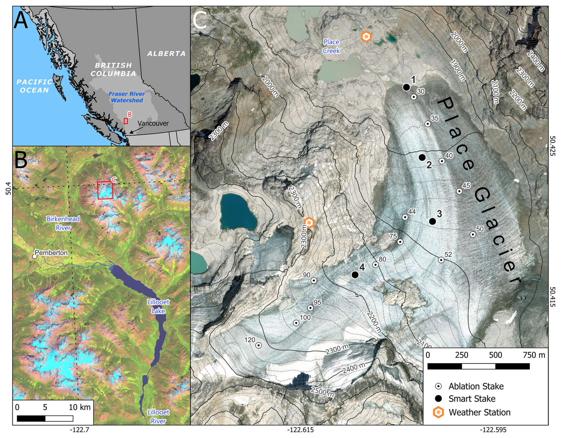
Figure 1 (A) Map of British Columbia highlighting the Fraser River watershed with the extent of panel (B) shown as a red square; (B) Location of Place Glacier in relation to Pemberton and Lillooet Lake with a false-color shortwave infrared 2024 seasonal mosaic from Sentinel-2 satellite imagery as a basemap; (C) Location of ablation stakes, smart stakes, and weather stations on Place Glacier with an 2 August 2024 orthoimage from aerial photography and lidar derived contour lines.

2 Place Glacier

Place Glacier (Randolph Glacier Inventory ID RGI60-02.01104) is located approximately 20 km northeast of Pemberton in the Southern Coast Mountains of British Columbia (RGI Consortium, 2017). This gently sloping glacier has minimal crevassing and negligible surface velocities, except in the areas of steeper topography, making it an ideal site for testing the smart stakes (Fig. 1). Place Glacier is one of 61 World Glacier Monitoring Service (WGMS) reference glaciers worldwide and has one of the most complete mass balance records in Canada (WGMS, 2024). The glacier has been the subject of multiple glaciology research studies (Ayala et al., 2015; Donahue et al., 2023; Moore and Demuth, 2001; Mukherjee et al., 2023; Munro and Marosz-Wantuch, 2009; Richards and Moore, 2003; Shea et al., 2009; Wood et al., 2011) and continues to have a mass balance program run by Natural Resources Canada (NRCan).

Place Glacier is part of the Fraser River watershed, and meltwater from the glacier flows into the Birkenhead River, which enters the Lillooet River before it enters the Fraser River (Fig. 1). The Place Creek watershed is about 14 km² and ranges in elevation from 452 to 2588 m above sea level (m a.s.l.). Place Glacier is the only glacier in this watershed and the glacier's surface area decreased from 3.55 km² in 1985 to 2.53 km² in 2021, representing a 29 % loss in 36 years (Bevington and Menounos, 2022).

3 Smart stake design

The smart stakes measure the distance to the glacier surface and also record air temperature and relative humidity. Our design priorities for the smart stakes include: (1) low power consumption; (2) multiple sensor compatibility; (3) reliable satellite telemetry; (4) small size and mass; and (5) low total cost.

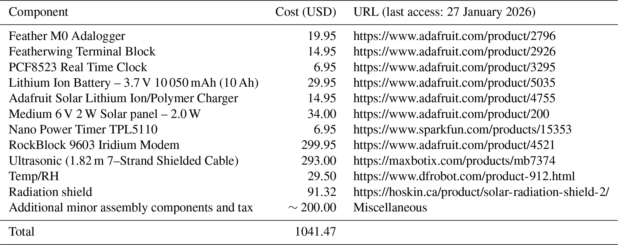
The smart stakes use an Arduino-compatible Adafruit© Feather M0 Adalogger microcontroller, hereafter referred to as the M0 (Adafruit Feather M0 Adalogger, 2025). Arduino is an open-source electronics platform based on easy-to-use hardware and software, widely used for prototyping interactive projects and embedded systems (Arduino, 2025). The M0 runs the ATSAMD21G18 ARM Cortex M0 processor, clocked at 48 MHz and has 3.3V logic (Adafruit Feather M0 Adalogger, 2025). The M0 is compatible with multiple analog and digital communication protocols (e.g. I²C, Analog, SDI-12, etc.), has a built-in micro-SD card reader, can be powered via USB or battery, and contains both FLASH (256 K) and RAM (32 K) memory. Our smart stake data logger includes a screw terminal breakout board for the M0, a real-time clock, solar charger, power management chip, and the satellite modem (Table 1, Fig. 2).

The power consumption of the Arduino system depends on the tasks assigned (e.g. waking up, checking the time, powering up and reading sensors, reading and writing data, and sending messages). Between measurements, the M0 can achieve low power consumption via a “deep sleep” command that is in the range of ∼4 mA (Adafruit Industries, 2023). Our smart stakes, however, do not use deep sleep commands, as we found that power consumption with these libraries remained too high and that they would often fail over long periods. We instead incorporate a SparkFun TPL5110 Nano Power Timer into the design; this board serves as an intermediary between the battery and the M0. The TPL5110 turns off the system, including the M0, between measurements, reducing sleep current to ∼35 nA ($\mathrm{3.5}\times {\mathrm{10}}^{-\mathrm{5}}$ mA) and ensuring that the entire Arduino system is reset for every measurement, mitigating the risk of Arduino failure over long periods. In a scenario where the M0 wakes up every 15 min for 10 s to take a measurement at ∼90 mA and communicates every 2 h at ∼245 mA for 2 min, the non-TPL version would consume 215 mAh d⁻¹, whereas the TPL version would only use 120 mAh. This difference in power consumption translates to usable battery life of about 47 and 82 d, respectively, with a 10 000 mAh Lithium Polymer (LiPo) battery and no solar panel. One disadvantage of the TPL chip is that measurements are collected approximately every 15 min. We cannot control how long it takes to send each Iridium message, it varies from seconds to minutes, and therefore, we cannot accurately estimate the battery lifetime.

The smart stakes have a small 6 V, 2 W solar panel that charges a 10 000 mAh 3.7 V LiPo battery. The charging efficiency of LiPo batteries is affected by both cold (<0 °C) and warm (>40 °C) temperatures. If the data logger runs out of power, the smart stake will stop working. In cases where the battery starts to charge again (temperatures warm, solar panel becomes snow-free), the TPL5110 is designed to restart the smart stake, and operations will resume. This feature adds resilience to extended periods with little or no charging in the winter. The total overall cost of the smart stake is approximately USD 1100. Most of this cost is made up of the Iridium modem and the ultrasonic sensor (Table 1). This cost is only a fraction of typical costs for a real-time AWS, which are typically in the range from USD 10 000 to 20 000.

Table 1 Primary components of the smart stakes with prices in USD from 6 June 2025. This list does not include a detailed breakdown of the minor components nor the ablation pole hardware.

3.1 Sensors

The smart stakes are equipped with ultrasonic, air temperature and relative humidity sensors. The ultrasonic sensor is the MaxBotix MB7374 HRXL-MaxSonar-WRST7, which is an inexpensive high precision range-finder that operates on low-voltages. It is specifically optimized for measuring snow and similar sensors have recently been used successfully by Wickert et al. (2019). The authors tested the sensor on multiple glaciers around the world, although without satellite telemetry, and provided useful recommendations for future field deployments that we were not aware of at the time of our installation. Wickert et al. (2019) recommend the MaxBotix MB7388, and also tested the MB7060, MB7389, and MB7386. A comprehensive comparison of the available sensors from MaxBotix was not done in this study.

Since the speed of sound increases by about 0.6 m s⁻¹ °C⁻¹, the ultrasonic has temperature compensation built into the sensor (HRXL-MaxSonar-WRS Datasheet, 2025). MB7374 can measure distances between 0.5 and 5 m. Factory data sheets report reading-to-reading stability of 1 mm at 1 m distance, and an overall accuracy of 1 % or better. Sensor values were tested against manual distance measurements on the glacier (Fig. S1 in the Supplement). The sensor operating temperature ranges from −40 to +65 °C and the input voltage requirement is 2.7 to 5.5 V. We sample the distance to the glacier 10 times at a frequency of 1 Hz and report the median of the 10 measurements every 15 min. The sensor is powered for 10 s before the first measurement.

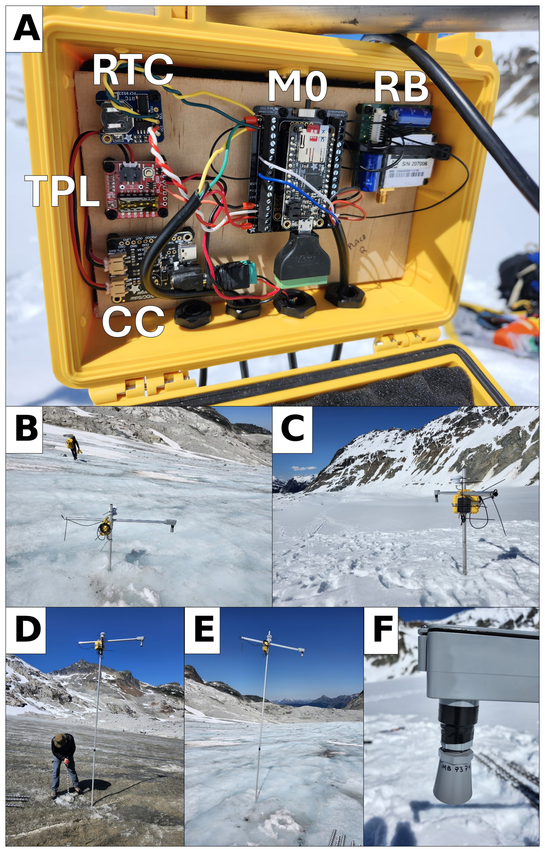
Figure 2 Photographs of the smart stakes on Place Glacier. (A) Place 2 station wiring with M0 (Feather M0), RB (RockBlock 9603), RTC (Real-time Clock), TPL (TPL5110 Nano Power Timer), CC (Charge Controller), and battery (behind the wooden board); (B) Place 2 on 16 July 2024; (C) Place 2 on 9 May 2024; (D) Place 1 on 16 July 2024; (E) Place 2 on 16 July 2024; (F) MaxBotix Ultrasonic Sensor (MB7374 HRXL-MaxSonar-WRST7).

The built-in temperature compensation resides inside the ultrasonic casing, which heats up in the sun. This sensitivity can manifest as variable distance measurements depending on the solar heating of the sensor. Typically, this can be corrected with independent air temperature measurements, however the MB7374 only reports the corrected distance, not the raw time of flight data and thus we cannot correct the data in post processing. The sensor can use a separate air temperature sensor to correct for this; however, this can only be done using a dedicated air temperature sensor that is soldered directly to the ultrasonic and this option was not available to us during the study. We do, however, include a separate DFRobot SEN0148 temperature and humidity sensor that uses the Sensirion SHT31-ARP chip. It is a fully calibrated, linearized, and temperature compensated analog output with input voltage requirements from 2.4 to 5.5 V. Operating temperatures are between −40 and +125 °C. Typical reported accuracies from the manufacturer are ±2 % RH and ±0.3 °C. The accuracy decreases to ±1.3 °C at the limits of the temperature range. We did not independently test the air temperature sensor accuracy. We found that the performance among the air temperature recorded at each smart stake deployed on the glacier had Pearson Correlation values greater than 0.96 between the observed daily air temperatures (Fig. S2).

3.2 Telemetry

Local low frequency radio, cell networks, and satellite networks are options for sending data from the field (Cremona et al., 2023; Kodali, 2017). Due to the remote location of our study area, we use satellite telemetry. Satellite options include either geostationary (e.g. GOES) or low earth polar-orbiting satellites (e.g. Iridium). Geostationary satellites offer a low financial cost per message; however, the upfront cost of the modem is high. Geostationary satellite telemetry also requires the modem to be directly pointed at the satellite which can be a challenge for fast-flowing glaciers or those situated within rugged topography, or in situations where the smart stake could slowly tip over while melting out. We use the Iridium satellite constellation due to the short wait times for satellite connectivity, flexible communication, and relatively low cost hardware (Gomez et al., 2021; IridiumSBD v2.0, 2024). The downside to Iridium is the cost per message structure and often 2–5 min wait times for messages to successfully transmit.

Messages are sent from the smart stakes to GroundControl©, a commercial service that brokers Iridium messages. We forward compressed messages as HTTP POST to a PostgreSQL database on a DigitalOcean© Server. Monthly line rentals are USD 16 per unit, and the number of credits used per message varies depending on the size of the message. Credits vary in cost based on purchase volume from USD 0.06 to 0.15 each. One credit is used per 50 bytes of data, and the maximum message size is 340 bytes. Two hours of hourly data from our stations translates to about 47 bytes which, in our case, results in a total monthly transmission cost of USD 36 per smart stake. The database can data be queried and visualized using open-source software (Bevington, 2025; Chang et al., 2025).

3.3 Installation

The ablation poles are made of two 2.44 m sections of 1-inch aluminum pipe joined by an aluminum coupler for a total length of 4.88 m. Previous work describes these poles and their overall performance for summer ablation monitoring (Beedle et al., 2014). A 1.2 m length cross arm of the same pipe is mounted near the top using readily available pipe couplers. The poles are drilled into the glacier so that the ultrasonic sensor is ∼0.8 m above the glacier surface at the start of the ablation season. For Sites 1–3, the snowpack was thin enough during the initial installation to drill the poles into the underlying ice, but thick snow at Site 4 prevented drilling the poles into the underlying ice.

The data logger is inside a Pelican 1120 Protective Case (Interior $L\times W\times D=\mathrm{18.5}\times \mathrm{12.1}\times \mathrm{8.5}$ cm), and the solar panel is mounted to the case using a metal hose clamp. The case is hooked onto the cross arm of the ablation stake using its handle and secured in place with a hose clamp. The ultrasonic sensor has a 19 mm thread and is mounted to a 90° electrical box, which is mounted to the aluminum cross arm. To limit the edge effects of the ablation stake in the footprint of the sensor, we positioned the ultrasonic sensor about 0.8 m away from the ablation stake. The T $/$ RH sensor is inside a radiation shield that is secured to the top of the main ablation stake.

4 Data and methods

In this paper, we combine in-situ and geospatial data to assess the utility of smart stakes by building a distributed glacier melt model using the smart stake data and testing the model against two independent validation datasets (Fig. 3).

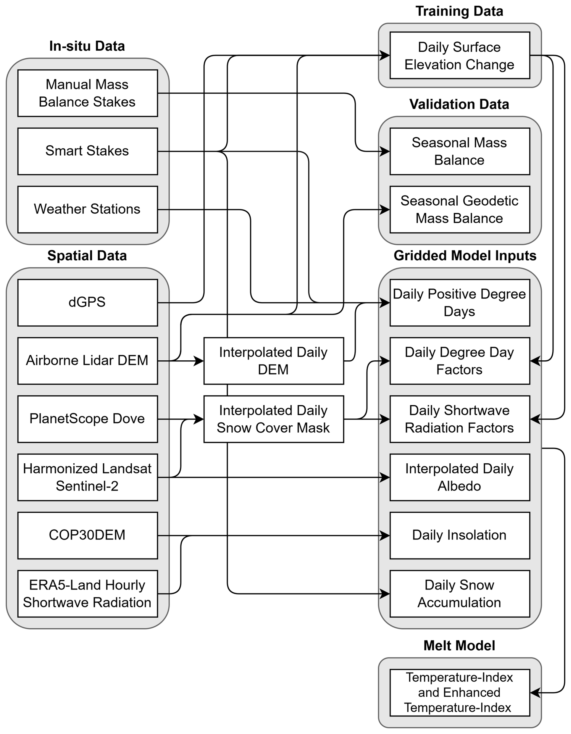
Figure 3 Flowchart of the workflow to prepare the gridded model inputs and the validation datasets using in-situ and spatial datasets.

4.1 In-situ data

We use in-situ data from: (1) the new smart stake network; (2) three AWS; and (3) thirteen manual mass balance stakes (Table 2).

Table 2 Metadata for the three weather stations, four smart stakes, and 13 WGMS stakes, see Fig. 1 for site locations.

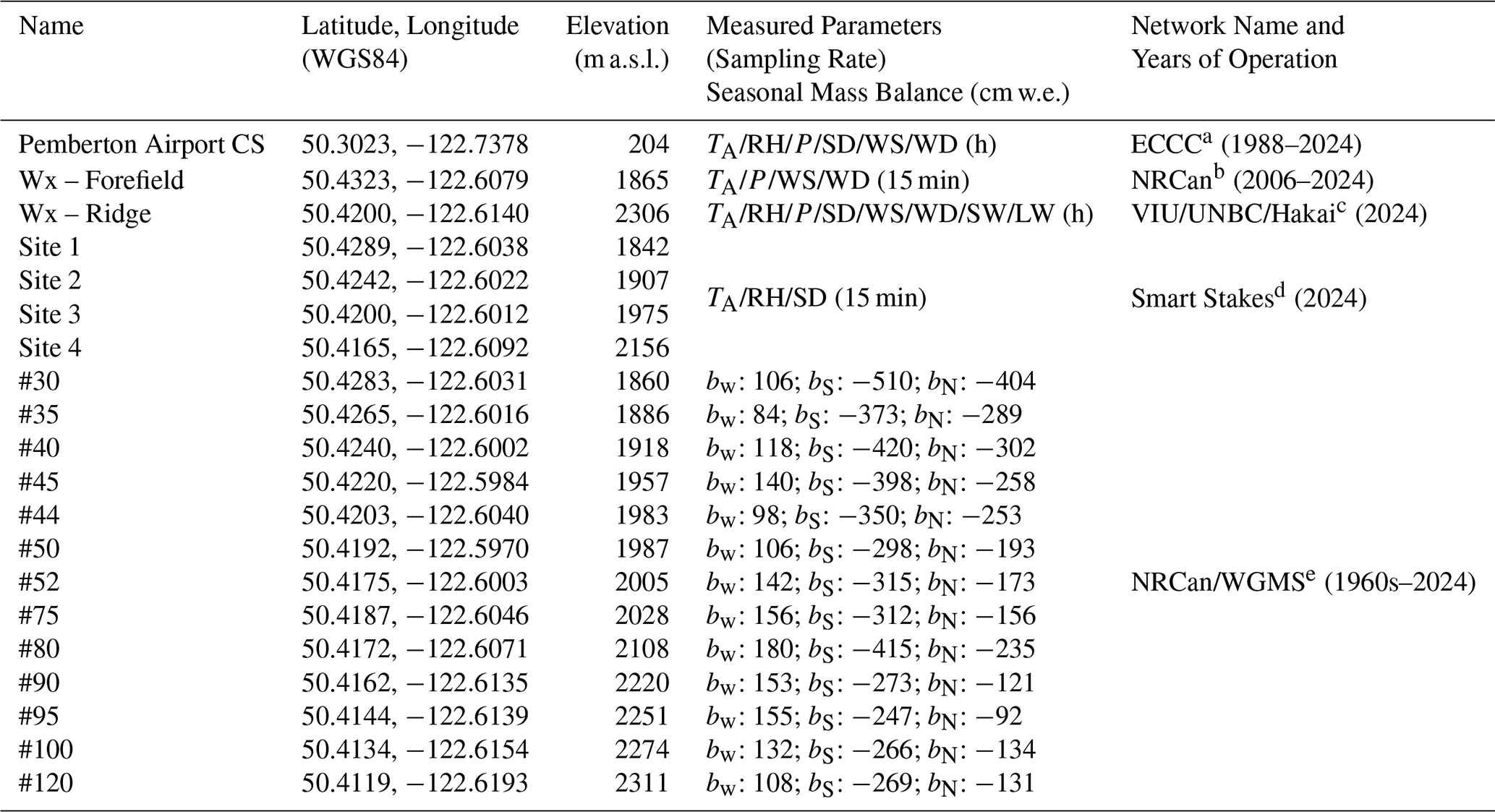
Air temperature; RH: Relative humidity; P: Air pressure; SD: Snow depth; SWE: Snow water equivalent; WS: Wind speed; WD: Wind direction; SW: In and out shortwave radiation; LW: In and out longwave radiation; h: Hourly; b_W: Winter Balance; b_S: Summer Balance; b_N: Net Balance; NRCan: Natural Resources Canada; VIU: Vancouver Island University; Hakai: Hakai Institute; ECCC: Environment and Climate Change Canada; ^a Data access at time of analysis: https://climate.weather.gc.ca/historical_data, last access: 27 January 2026; ^b Personal communication; ^c Data access at time of analysis: http://viu-hydromet-wx.ca/graph/, last access: 27 January 2026; ^d Data access at time of analysis: https://bcgov-env.shinyapps.io/nbchydro/, last access: 27 January 2026; ^e Personal communication.

4.1.1 Smart stakes

The four smart stakes installed at the end of the accumulation season (8 and 9 May 2024) cover an elevation range from 1842 to 2156 m a.s.l. (Fig. 1, Table 2). We accessed the glacier by helicopter, which adds financial considerations to the frequency of field visits and the cost benefit of real-time data. The uppermost region of the accumulation area was not instrumented due to field safety and logistical constraints during the May 2024 fieldwork, namely poor visibility at higher elevations caused by low cloud. To prevent the stakes from melting out and tipping over, we redrilled the stakes on 16 July 2024, and again on 21 September 2024. Smart stake data from 8 May to 14 November 2024, are used in this study. Site 1 is located near the glacier terminus, where the north facing glacier's slope is 10°. Site 2 is 535 m away on a gentler 9° slope with the same north aspect. Site 3 is on a flatter 5° northward flowing bench, right before the glacier turns westward up glacier. Site 4 is on a steep 16° east-northeast ramp that leads to a high elevation bowl (Fig. 1, Table 2).

The time series of glacier surface observations recorded by the smart stakes require filtering, gap filling, and datum corrections. The ultrasonic sensor reports the maximum range of the sensor (5 m) if there is signal interference during precipitation events, drifting snow, or high winds. Objects closer than the minimum detection range (e.g. rime ice build-up on the sensor, spider webs, or other obstructions) are reported as 0.5 m. Bad data can also be caused by the stakes themselves leaning over or turning. We infill missing data for periods of less than 5 h using linear interpolation. The distance values are converted to cumulative elevation change by adjusting the time series after each time the stake is redrilled, and the cumulative elevation change is corrected to cumulative meltwater volume using field observations of snow density (summer 570±20 kg m⁻³) and ice density (910±10 kg m⁻³) reported by Pelto et al. (2019).

4.1.2 Weather stations

Three weather stations are used in this analysis (Fig. 1, Table 2). The first, “Wx-Forefield”, is a weather station run by NRCan located 412 m down valley from the glacier terminus located on bedrock in the glacier forefield. The second, “Wx-Ridge”, is a new weather station installed in early summer 2024 on an alpine ridge above the glacier. The third, “Pemberton Airport CS”, is an Environment and Climate Change Canada (ECCC) weather station near Pemberton. The weather stations, in combination with the air temperature recorded at the smart stakes, are used to investigate and develop daily lapse rates which allow the computation of gridded positive daily degree day (PDD) models.

4.1.3 Manual stakes

Data from thirteen manual ablation stakes collected by NRCan as part of the WGMS are used as validation data in this study (Fig. 1, Table 2). The stake positions and degree of melt are surveyed in autumn every year and snow depth and density are measured in the spring (WGMS, 2024). We only use the manual ablation stake field data for years 2023–2024. Field data collection occurred on 7 October 2023, 19–20 April 2024, and 20–21 September 2024. Snow densities on 19–20 April 2024, ranged from 419 to 472 kg m⁻³, with an average of 434 kg m⁻³. The highest recorded densities were located at lower elevations on the glacier. The winter, summer, and net mass balance for each manual stake are reported in Table 2. This data is used as an independent validation dataset for melt modelling (Fig. 3).

4.2 Geospatial data

4.2.1 Airborne lidar

Airborne lidar and air photo data is available for 7 October in 2023, and 11 May, 6 June, 4 July, 2 August, 31 August, 16 September, and 12 October in 2024. These flights are part of the Airborne Coastal Observatory glacier monitoring program (Donahue et al., 2023; Menounos et al., 2019, 2025). These acquisition dates overlap with the smart stake deployments, and the elevations can be compared directly to the smart stake data. Slope and aspect were calculated using the 31 August 2024 digital elevation model (DEM) in QGIS 3.34 (QGIS Development Team, 2023).

The DEMs were resampled to a 5 m grid using bilinear interpolation, and co-registration of the DEM stack was done using the “xdem” python package with stable exposed and snow-free bedrock nunataks (Dehecq et al., 2022). We identified bedrock nunataks in a 11 May 2024 air photo and assumed that they were stable throughout the time series. Stable ground was used to determine the three-dimensional correction vectors. This was done with methods from Nuth and Kääb (2011) that estimate horizontal and vertical translations by iterative slope and aspect alignment. In addition, a 2D polynomial correction was applied to account for any elevation bias.

4.2.2 Geodetic mass balance

We calculate the net geodetic mass balance from the repeat lidar of Place Glacier by combining the winter and summer geodetic mass balances (Pelto et al., 2019). The winter balance is calculated as the difference between the peak spring snowpack on 11 May 2024, and the previous autumn melt surface on 7 October 2023. The summer balance is the combination of the loss of the winter snowpack, and the loss of glacier ice, measured as the difference of the 7 October 2023, surface and the 16 September 2024, surface (Fig. S4). The elevation change is then converted to snow water equivalent (m w.e.) using the same snow and ice densities as described above (Pelto et al., 2019).

4.2.3 Differential GPS

Since there is no stable ground near the smart stakes themselves, a relative datum could not be established through traditional survey methods. As such, the most reliable way to ensure the accuracy of the smart stakes is by correcting the data to a geodetic datum using differential GPS (dGPS) measurements. Unfortunately, we only have high resolution dGPS measurements from 21 September 2024, for Sites 3 and 4. We use the Emlid Reach RS2+ dGPS system, that produced spatial accuracies of 0.006 m and vertical accuracy of 0.01 m. Points were recorded upon arrival and after resetting the stake.

4.2.4 Optical satellite imagery

We combine surface reflectance data from the publicly available Harmonized Landsat Sentinel-2 Version 2.0 (HSL) with commercially available data from the PlanetScope Dove constellation (PS) to map snow and ice cover on the glacier over time.

The HLS dataset combines imagery from the Operational Land Imager (OLI) aboard Landsat 8 and Landsat 9 satellites with the Multi Spectral Instrument (MSI) aboard the three Sentinel-2 satellites (2A, 2B and 2C). The HLS has an average revisit time of 2–3 d at 30 m resolution. The imagery was accessed programmatically from Microsoft Planetary Computer (Microsoft Open Source et al., 2022) using the “rstac” package (Simoes et al., 2021). Between 1 May –31 October 2025, there were 34 images available from Landsat and 57 from Sentinel-2. PS is a constellation of commercial CubeSat satellites that offer near-daily 3.8 m resolution optical imagery and have been used in other glaciological studies (Liu et al., 2024; Tarca et al., 2023). The “planetR” package was used to bulk download 73 scenes that intersect the bounding box of the area of interest with less than 20 % cloud cover (Bevington, 2023). We manually filtered out partial or cloudy images, leaving 15 Landsat, 25 Sentinel-2, and 31 PlanetScope Dove images, for a total of 71 images. These images represent 47 unique dates due to acquisitions on the same day by different sensors.

We use the near infrared (NIR) band with a threshold of 0.4 to differentiate between snow and ice (Riggs et al., 1994; Zhang et al., 2019). This simple band threshold method is sufficient for discrimination of snow from glacier ice (Fig. 4). This method is not well suited, however, for more complex workflows that could include, for example, off-glacier areas, supraglacial lakes, or clouds.

Surface albedo was calculated for the HLS dataset using methods from (Feng et al., 2024). We then interpolate both the satellite-derived snow cover and albedo data to a daily resolution by linear gap-filling of the data.

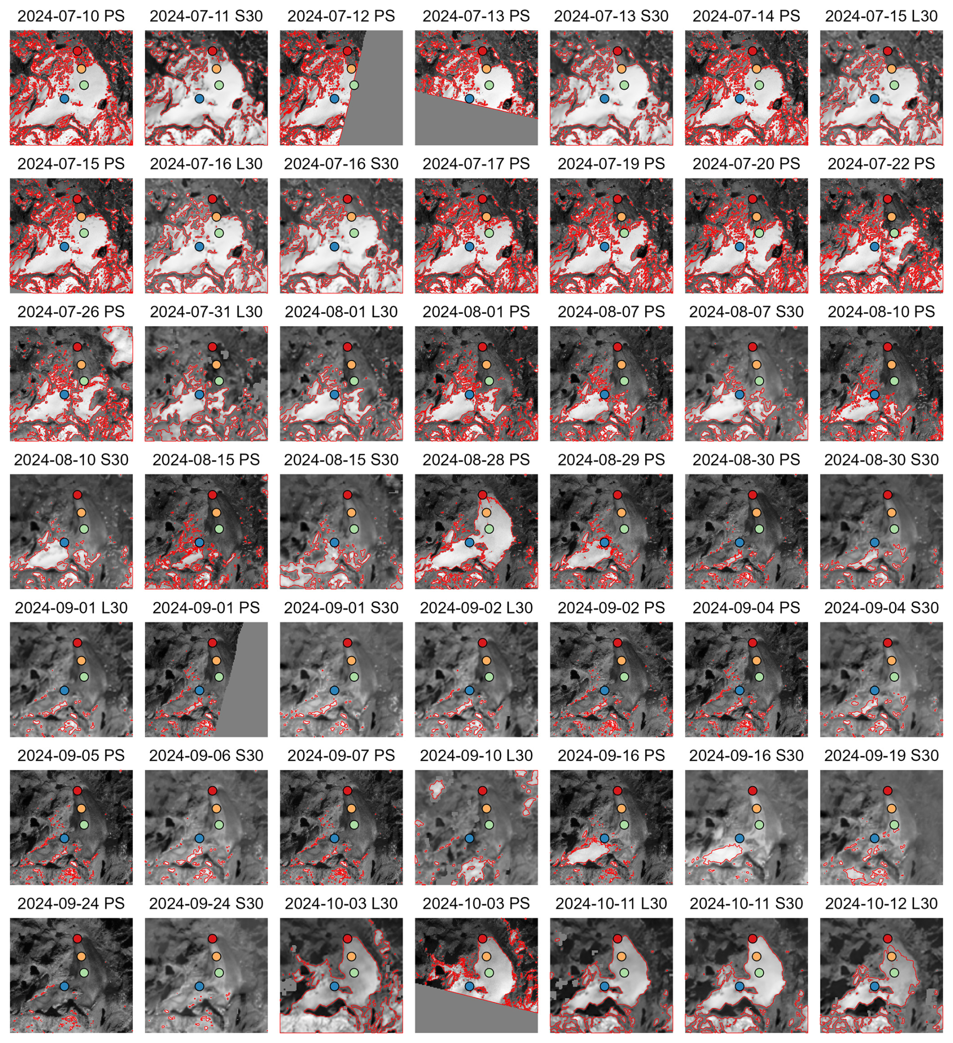
Figure 4 Selected Landsat 8/9 (L30), Sentinel-2 (S30), and PlanetScope Dove (PS) near infrared images of Place Glacier. The red outline is the snow mask determined from a 0.4 threshold of the near infrared band, and the points are the smart stake locations (Sites 1–4 are colored red, orange, green, and blue, respectively).

4.2.5 Incoming shortwave radiation

The ERA5-Land reanalysis dataset provides gridded estimates of essential climatic variables at 9 km resolution from 1950 to present (Muñoz-Sabater et al., 2021). We use the surface solar radiation downwards (SSRD) data, also known as the incoming shortwave radiation, which is an important component of the energy input that drives glacier melt (Litt et al., 2019). The hourly SSRD dataset is in J m⁻². This variable comprises both direct and diffuse solar radiation. We derived gridded daily mean insolation values in W m⁻² by resampling the SSRD data to a daily resolution. We then corrected this value for topographic shading using the methods published by Steger et al. (2022). Specifically, we employed the COP30DEM in the shading calculation. The COP30DEM (Copernicus Global 30 m Digital Elevation Model) is a global, 30 m resolution representation of the Earth's surface elevation derived primarily from the TanDEM-X radar mission data acquired between 2011 and 2015 (European Space Agency, 2024). We use the COP30DEM over the airborne lidar data because a large spatial domain is required for the shading calculations.

4.3 Temperature-index models

4.3.1 Model formulation

In order to distribute our smart stake glacier melt observations to the entire glacier, we use a simple temperature-index models since we lack important observational data for an energy balance model (Beedle et al., 2014; Braithwaite and Zhang, 2000; Carenzo et al., 2009; Pellicciotti et al., 2005; Shea et al., 2009; Wickert et al., 2023). We test both the Temperature-Index (TI) and the Enhanced Temperature-Index (ETI) glacier melt models. The TI model operates on the simple assumption that air temperature is well correlated with shortwave radiation, both being the primary drivers of melt. When air temperature exceeds a threshold value, commonly set at 0 °C, melt occurs (Braithwaite and Zhang, 2000). The amount of melt is calculated using melt factors for ice and snow, which represent the amount of melt per degree Celsius per day, commonly expressed in meters of water equivalent per degree Celsius per day (m w.e. °C⁻¹ d⁻¹). The TI model can be expressed as Eq. (1):

$$\begin{array}{}\text{(1)}& M=\left\{\begin{array}{ll}\text{TF}T& T>T_{\mathrm{T}}\\ \mathrm{0}& T\le T_{\mathrm{T}}\end{array}\right.\end{array}$$

Where M is melt in m w.e., T is the mean daily air temperature (°C), and TF is an empirically-derived coefficient for the air temperature melt factor, expressed in m w.e. °C⁻¹ d⁻¹. T_T is a threshold temperature above which melt is assumed to occur, in this case we use 0 °C. This model is simple and allows an initial estimate of melt and does not account for more complex processes like incoming solar radiation, wind, humidity, or albedo.

We also test the ETI model from Pellicciotti et al. (2005). The model offers improvements over TI models by including incoming shortwave radiation, and albedo. The model is expressed as Eq. (2):

$$\begin{array}{}\text{(2)}& M=\left\{\begin{array}{ll}\text{TF}T+\text{SRF}\left(\mathrm{1}-\mathit{\alpha }\right)\mathrm{SR}+\mathrm{SF}& T>T_{\mathrm{T}}\\ \mathrm{0}+\mathrm{SF}& T\le T_{\mathrm{T}}\end{array}\right.\end{array}$$

Where M is melt in m w.e. and α is albedo. SR is incoming shortwave radiation in W m⁻² and SRF is an empirical coefficient for the shortwave radiation melt factor, expressed in m w.e. W⁻¹ m⁻². SF is the total daily snowfall in m w.e., the other variables are the same as in Eq. (1).

We calculate TF and SRF in three different ways: (1) TF is calculated from daily PDD and daily melt values (TF_DM); (2) TF is calculated from cumulative PDD and cumulative melt (TF_CM); and (3) TF and SFR are calculated from solving a multiple linear regression from the daily values (TF_MLRand SRF_MLR). The two first methods are used in the TI model, Eq. (1), and the third method is used in the ETI model, Eq. (2). Melt factors are often similar among stakes, and are often assumed to be constant over time, however in reality they have been shown to change day-to-day, highlighting then need for energy balance models.

4.3.2 Spatial model implementation

We distribute these models spatially by interpolating the gridded inputs to a daily resolution (Fig. 3). These include daily snow cover, air temperature, albedo, snow accumulation, and incoming shortwave radiation. This also allows for the calculation of the total melt volume from Place Glacier for the 2024 ablation season.

The seven 2024 lidar DEMs are interpolated to daily resolution from 11 May to 21 September 2024, using pixel-wise linear interpolation over the time series (Fig. S5). A daily gridded air temperature model is then estimated using daily air temperature lapse rates calculated from the smart stakes and weather stations. Six separate air temperature lapse rates are tested using daily data: (1) Using a normal lapse rate of −6.5 °C km⁻¹ from the ECCC station; (2) Linear model using all seven air temperature datasets; (3) Linear model using off-glacier stations; (4) Linear model using on-glacier stations; (5) 2nd order polynomial model using on-glacier stations; and (6) 2nd order polynomial model using only the upper stations (all but ECCC).

Previous work demonstrated the importance of understanding on- and off-glacier air temperatures, and the important local influence of the ice temperature and air flow dynamics within the katabatic boundary layer (Ayala et al., 2015; Shea et al., 2009; Shea and Moore, 2010). Our air temperature models do not explicitly account for effects occurring inside or outside the katabatic boundary layer, as we lack the required data to do so. The effects of the katabatic boundary layer may, however, be partially accounted for by using on-glacier stations in lapse rate calculations.

Snow and ice cover is interpolated to a daily resolution from the HLS and PS data by gap-filling the sparse time series with the last good measurement from spaceborne observations to infill the missing daily values. The daily snow cover mask is used to assign the empirical coefficients (TF and SRF) for snow and ice (Fig. 3). Accumulation is accounted for in the model using the observed accumulation at each stake and interpolated across the glacier using elevation.

The melt models are then applied to every pixel which is converted to a total seasonal melt volume (m³) by multiplying the estimated melt (m w.e.) by the pixel resolution (in m) and adding together the daily totals. The summer balance can then be calculated as the melt volume divided by the glacier area.

5 Results

5.1 Smart stake performance

The smart stakes performed without fault for Sites 1 and 3. Measurements of air temperature, relative humidity, and the distance to the glacier surface were recorded every 15 min and hourly data were sent over the Iridium satellite network. Site 2 experienced intermittent satellite communication, which we believe was caused by loose wiring. The full dataset, however, was preserved on the local SD card. Site 2's intermittent communication corrected itself mid-summer, but the stake stopped transmitting after our last field visit of the season on 25 September 2024. The cause of this issue remains unknown as the logger is on the glacier at the time of writing. Site 4 performed well for the ablation season but then suddenly stopped working on 11 September 2024, due to a corrupted memory card.

We redrilled the smart stakes on 16 July and on 21 September to prevent them from melting out. On the 21 September field visit, Sites 1–4 were found to be leaning at angles of 41, 31, 24, and 15°, respectively (Fig. 5); the day where tilting commenced remains uncertain. As a precaution, we remove data from late-August to 21 September when the stakes recorded significant accumulation during a period of air temperatures greater than 10 °C, when in reality the perceived accumulation was caused by the glacier surface becoming closer to the sensor while the stake was tipping over (Figs. 5, 7).

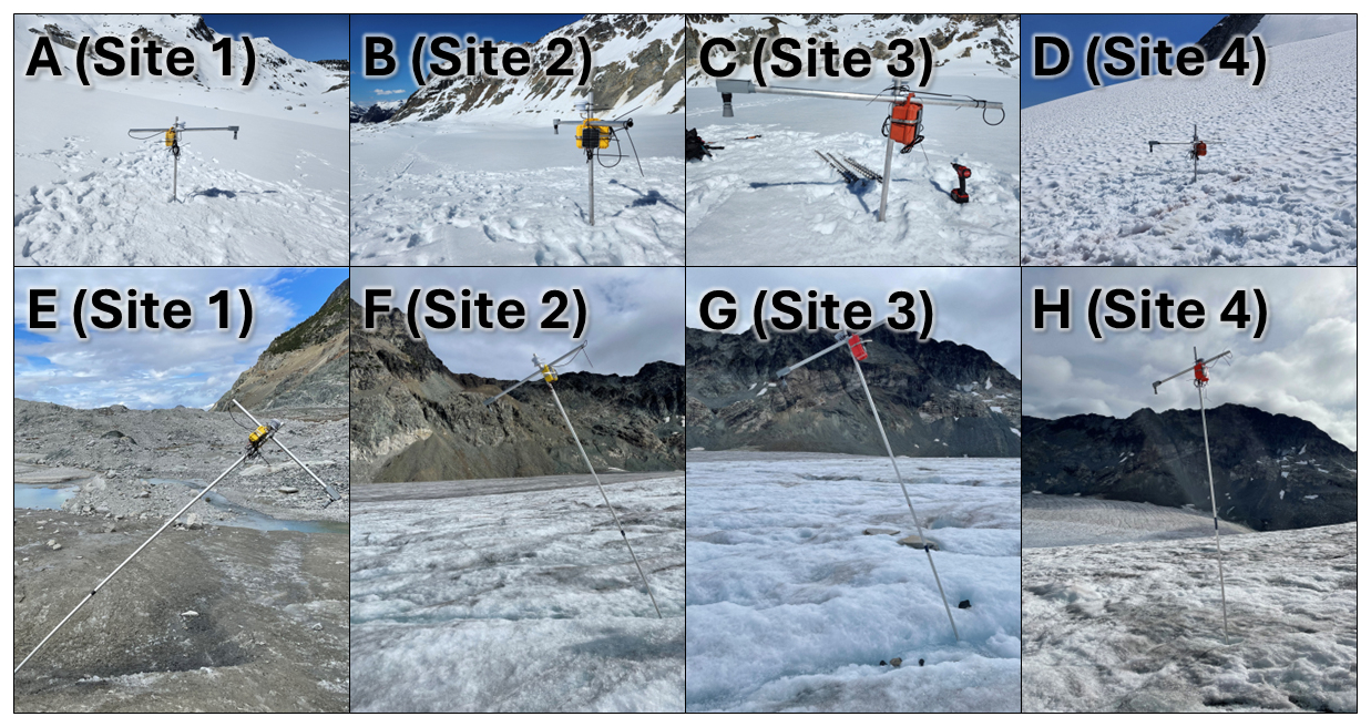
Figure 5 Site photos from left to right (Sites 1–4). Photos were taken on 16 July after being redrilled (A, B, C, D), and on 21 September when found melting over before being re-drilled or removed (E, F, G, H).

The MB7374 ultrasonic sensor performed well against in-situ calibrations (Fig. S1). The root mean square error (RMSE) between field measurements done with an avalanche probe and the sensor itself had an overall error of 0.046 m. The avalanche probe used had a 1 cm graduation, and the highest values (>3 m) have a larger uncertainty due to the challenge of seeing the exact measurement on the avalanche probe. The glacier melt surface also presents a challenge as it is a sloped and uneven surface. The MB7374 sensor was susceptible to solar heating, with an observed diurnal fluctuation of ±5.5 cm on hot sunny days (Fig. S3). This effect could be mitigated in the future by using the external temperature sensor correction inputs that are built into the sensor's functionality. To our knowledge it is not possible to do this after the fact with the MB7374 using the air temperature that we recorded since it does not report the time of flight, or the temperature compensation used. The nighttime temperatures are likely the most reliable due to the absence of solar heating of the sensor and the temperature compensation built into the ultrasonic should be closer to the actual air temperature.

5.2 Satellite derived snow cover

For Sites 1–4, the start of the snow free season occurred on 12 July, 14 July, 19 July, and 15 August 2024, respectively (Figs. 4, 6). Cloud cover during mid-August, late-September and early-October introduced gaps into the satellite image time series. The transient snowline gradually rose over the ablation season with a summer snowfall event observed on 28 August 2024 (Fig. 6). The accumulation area completely disappeared by 24 September 2024, and snowfall events became more frequent in October (Fig. 6). The accumulation area ratio (AAR), or the percent of snow cover on the glacier, was near zero for most of the month of September. A mid-summer snowfall event temporarily increased surface albedo, but the snow cover disappeared in a matter of days (29–30 August).

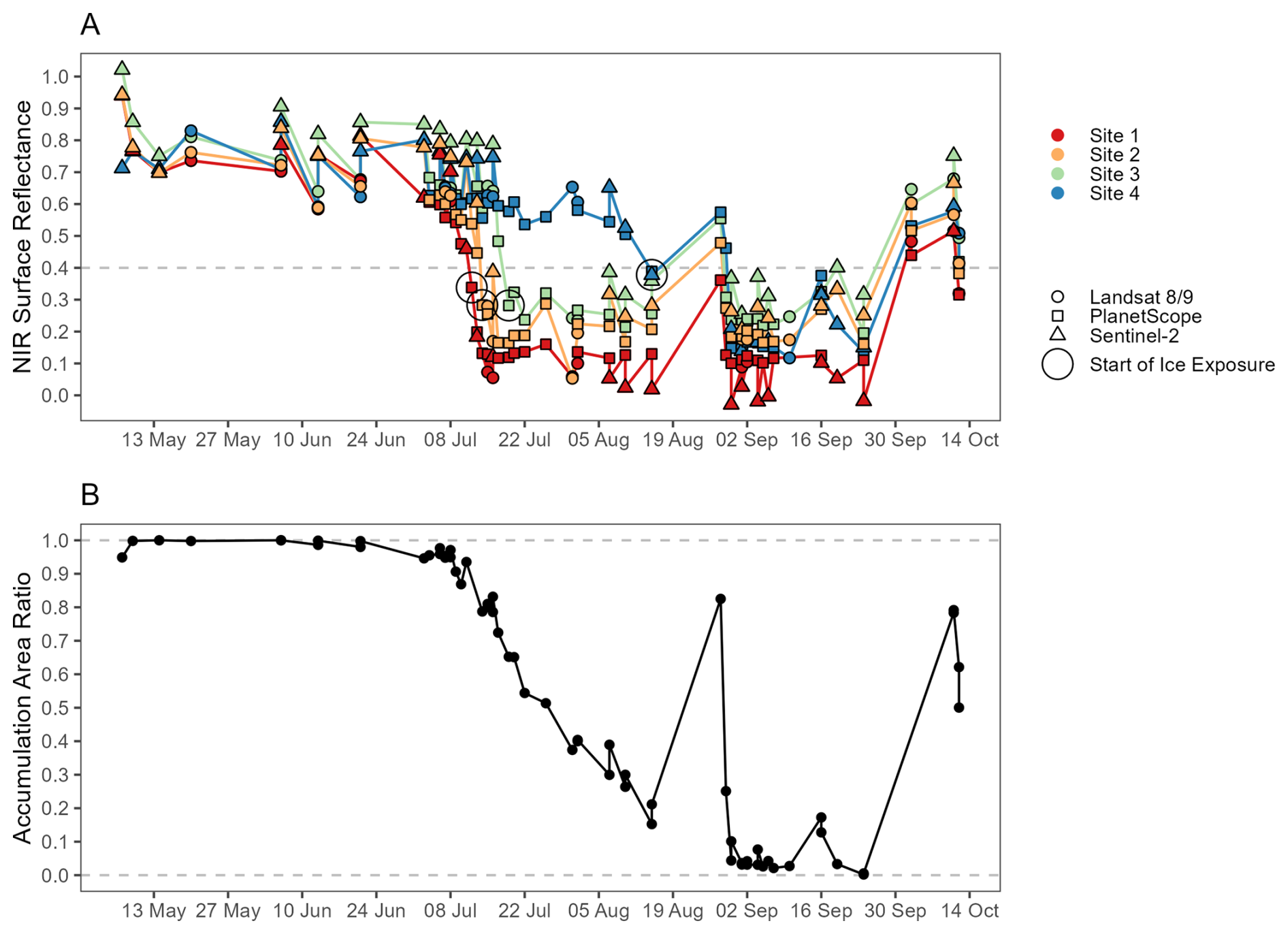
Figure 6 (A) Spectral time series of the NIR bands from PlanetScope for the smart stake locations. The black squares represent the first snow-free observation at that location. (B) Time series of the 2024 accumulation area ratio (AAR) for Place Glacier.

5.3 Time series data

The cumulative elevation change measured at each stake was adjusted to elevation above sea level using the 11 May lidar (Fig. 7). The RMSE between the lidar elevation and the valid smart stake measurements is 0.18, 0.11, 0.12, and 0.50 m for Sites 1–4, respectively. The largest differences are at Site 4, which may be due to the steeper glacier surface and possibly greater ice velocities, or due to the stake settling or tilting as it was not drilled into ice at the start of the season. The total lidar-derived cumulative elevation change of the glacier surface in 2024 was −6.4, −6.0, −5.3, and −5.5 m for Sites 1–4, respectively (Fig. 7). Unfortunately, as previously discussed, the smart stakes did not provide reliable elevation data during early September – the warmest period of the 2024 season – since they were slowly tipping over (Fig. 7). The repeat lidar proved critical for correcting the time series after the stakes tilted over, as we did not have dGPS measurements form the early season.

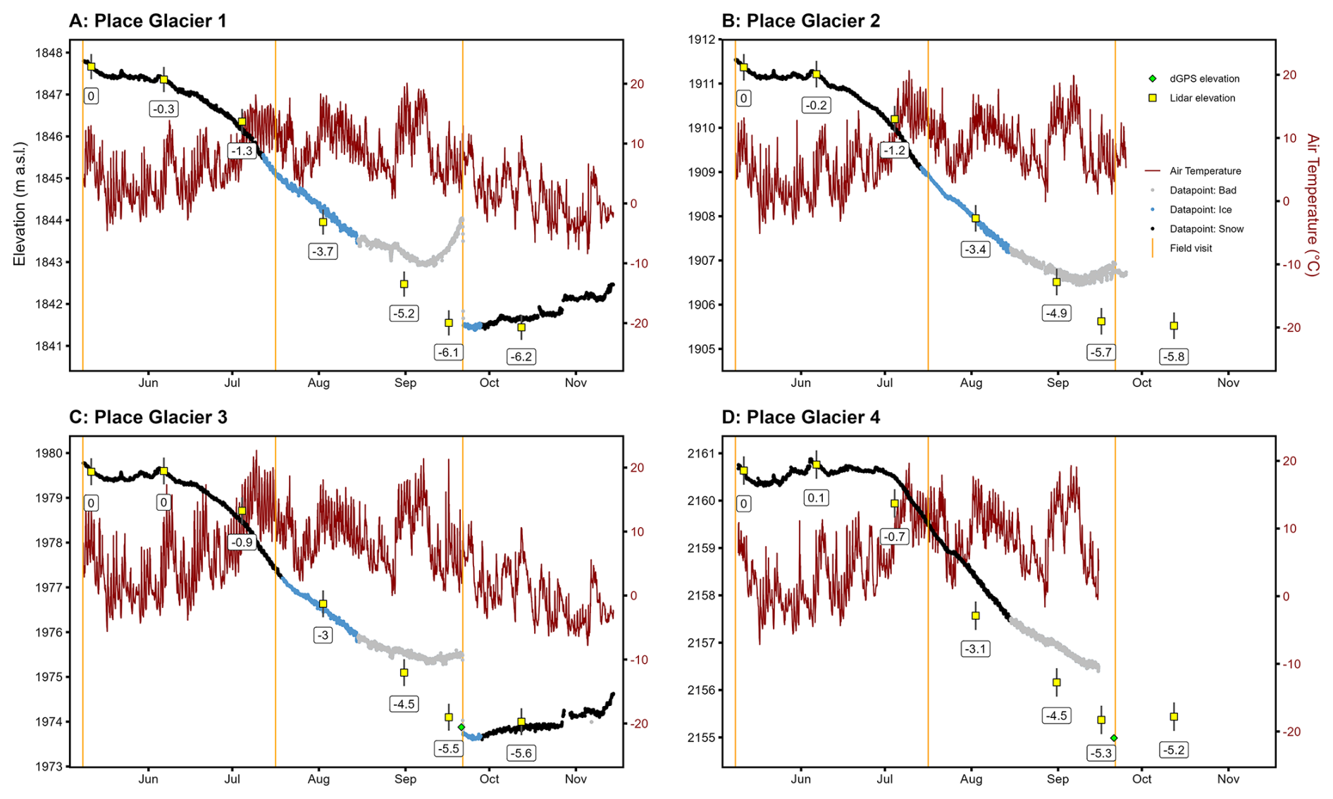
Figure 7 Time series of hourly glacier elevation and air temperature from the four smart stakes (A–D). Glacier elevation points are colored as snow (black), ice (blue), and bad data points (grey). Independent elevation datasets are shown: lidar (yellow square with 30 cm error bars and labels of the cumulative elevation change in meters) and differential GPS (green diamond).

5.4 Lapse rates

We calculated the mean daily air temperature lapse rates using six different methods, described above in Sect. 4.3.2. We recorded three heat events on the glacier, herein defined as times when the mean daily air temperature was above 10 °C (Fig. 8A). Daily air temperature lapse rates were generally normal (negative) when considering observed air temperatures (Fig. 8B). However, inverted (positive) lapse rates occurred on the glacier during warmer summer air temperatures (Fig. 8C). The minimum, mean and maximum lapse rates were: −9.3, −5.7, and −1.2 °C km⁻¹ for all stations; −7.6, −5.8, and −1.7 °C km⁻¹ for off-glacier stations and −14.4, −4.4, and +8.0 °C km⁻¹ for on-glacier stations, respectively.

As an example of the lapse rate performance, we consider observed lapse rates for 20 July 2024 (Fig. 8C). The three models that include the ECCC station do not perform well on the glacier (models 1, 2 and 3). Models 4, 5, and 6 visually capture the on-glacier air temperature relation. The polynomial lapse rates outperform the linear lapse rates on the training data but are more prone to overfitting. The polynomial models are also likely to perform poorly outside of the range of observations (e.g. high elevations where there are no stations). All lapse rate models are included in overall model performance evaluation against manual mass balance stakes and geodetic mass balance. Inverted (positive) lapse rates generally occurred on the glacier during warmer summer air temperatures (Fig. 8D). These inversions generally occur during warmer periods. Small variations exist among lapse rate models 2–6, whereas large variations are present when we consider using the ECCC data with a standard lapse of −6.5 °C km⁻¹ (Fig. 8E).

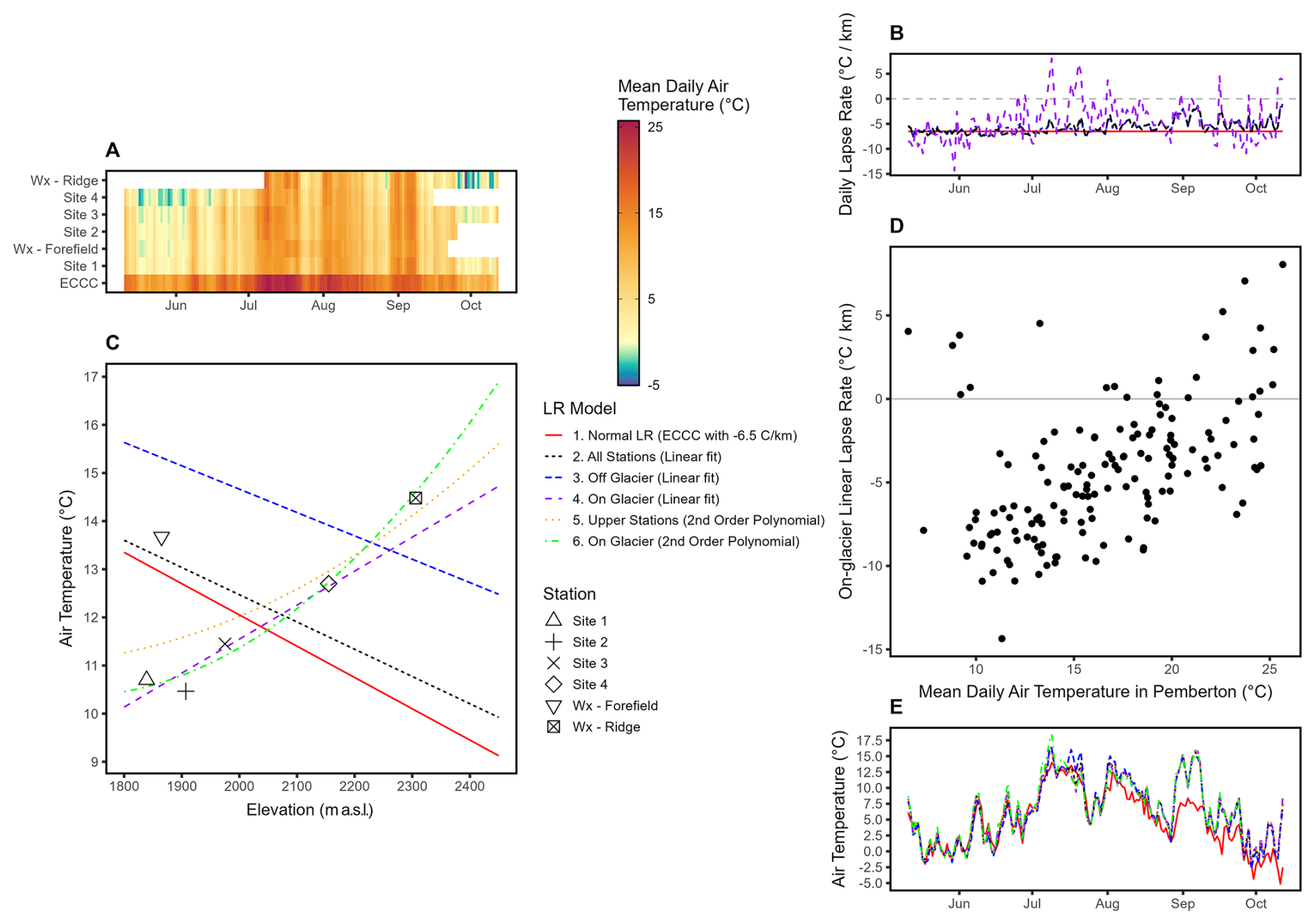
Figure 8 (A) Heat map of the mean daily air temperature from seven weather stations considered in this study; (B) Daily lapse rates using a linear model with three different station groups: All (All stations), Off Glacier stations, and On Glacier stations; (C) Comparison of observed and modelled air temperatures using different lapse rate models for 20 July 2024. The ECCC Station is not shown (204 m a.s.l. and 23.7 °C); (D) Scatterplot of on-glacier linear lapse rates and mean daily air temperature at the ECCC Pemberton station; (E) On-glacier air temperature at 2000 m elevation from the six air temperature models.

5.5 Melt factors

The empirically-derived cumulative air temperature melt factors for snow (TF${}_{{\mathrm{CM}}_{\mathrm{s}}}$) are −4.38, −4.42, −3.78, and −3.74 mm w.e. °C⁻¹ d⁻¹, for Sites 1–4, respectively (Fig. 9, Table 3). For ice (TF${}_{{\mathrm{CM}}_{\mathrm{i}}}$) they are −5.14, −5.30, and −4.19 mm w.e. °C⁻¹ d⁻¹, for Sites 1–3. The average TF${}_{{\mathrm{CM}}_{\mathrm{s}}}$ and TF${}_{{\mathrm{CM}}_{\mathrm{i}}}$ among all sites are $-\mathrm{4.08}\pm \mathrm{0.11}$ and $-\mathrm{4.87}\pm \mathrm{0.18}$ mm w.e. °C⁻¹ d⁻¹, respectively. The R² values exceed 0.98 for both ice and snow at all sites when derived from cumulative positive degree days (Fig. 9). These melt factors compare favorably to those derived from daily air temperature and melt data which average $-\mathrm{3.88}\pm \mathrm{0.09}$ for snow (TF${}_{{\mathrm{DM}}_{\mathrm{s}}}$) and $-\mathrm{4.79}\pm \mathrm{0.21}$ mm w.e. °C⁻¹ d⁻¹ for ice (TF${}_{{\mathrm{DM}}_{\mathrm{i}}}$) (Fig. 9, Table 3).

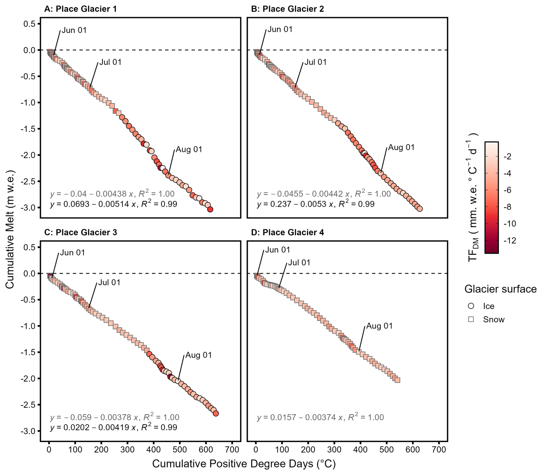
Figure 9 Scatterplot of the observed cumulative positive degree days and the cumulative melt for each site (A–D). The coefficients for snow and ice are shown on the plot in m w.e. °C⁻¹ d⁻¹. Points are colored by the daily melt factors in mm w.e. °C⁻¹ d⁻¹. The regression formula and R² values are in grey for snow, and black text for ice.

Using multiple linear regression (MLR) with daily melt, air temperature, shortwave infrared, albedo and snowfall in Eq. (2), we obtain air temperature coefficients for snow (TF_MLRs) and ice (TF_MLRi) were $-\mathrm{3.52}\pm \mathrm{0.26}$ and $-\mathrm{4.21}\pm \mathrm{0.62}$ mm w.e. °C⁻¹ d⁻¹, respectively. Whereas shortwave radiation coefficients for snow (SRF_MLRs) and ice (SRF_MLRs) respectively yield $-\mathrm{0.041}\pm \mathrm{0.006}$ and $-\mathrm{0.029}\pm \mathrm{0.025}$ mm w.e. W⁻¹ m⁻² d⁻¹ (Table 3).

Table 3 Melt factors for TI and ETI models.

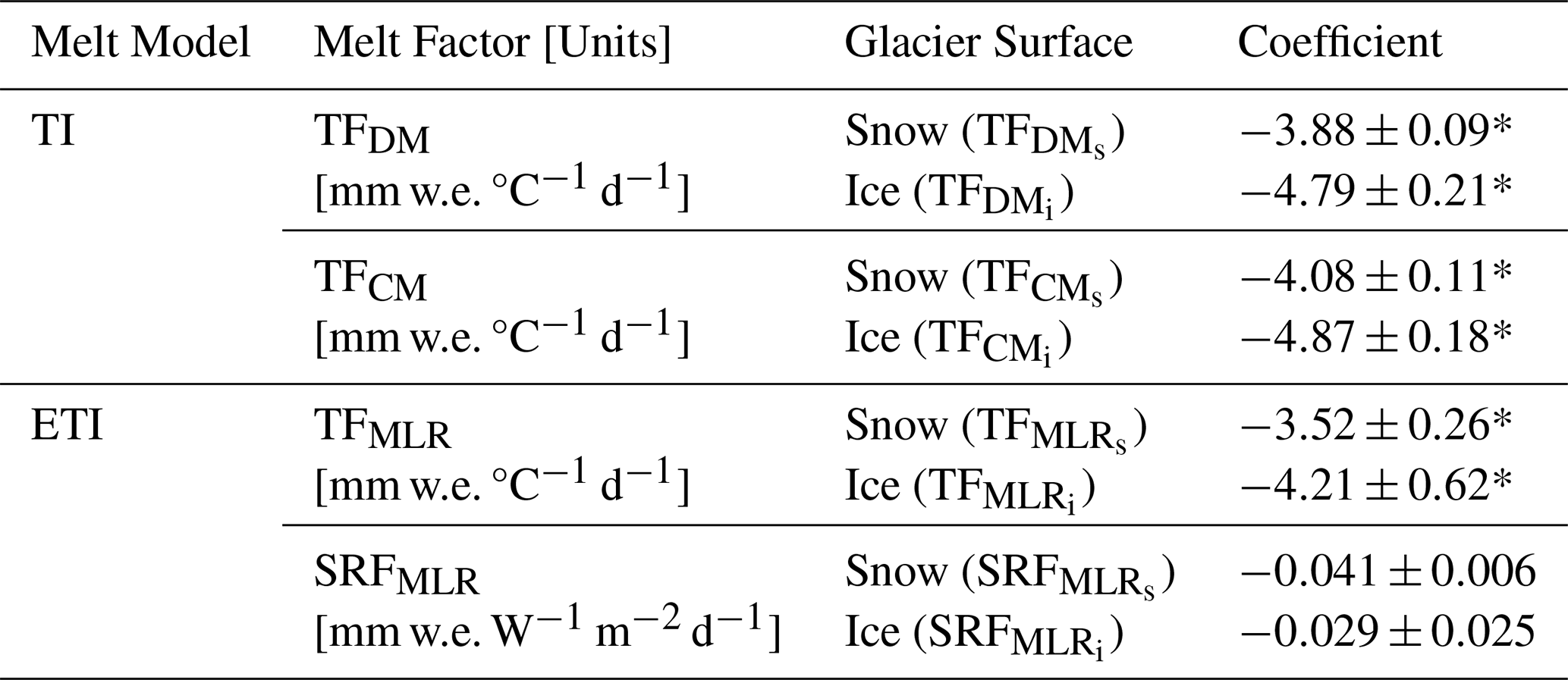
TI: Temperature-Index; ETI: Enhanced Temperature-Index; TF_DM: Temperature factor from daily melt; TF_CS: Temperature factor from cumulative melt; TF_MLR: Temperature factor from multiple linear regression; SRF_MLR: Shortwave radiation factor from multiple linear regression; ^* p value <0.05.

5.6 Model evaluation and selection

We test three melt model implementations with five air temperature lapse rates against both the network of four smart stakes and the network of independent manual seasonal ablation stakes (Figs. S6, S7, S8). The top three performing models at the manual stakes are the ETI with the upper station polynomial lapse rate (r²=0.634), the ETI with the on-glacier linear lapse rate (r²=0.632), and the off-glacier linear lapse rate (r²=0.624). We selected the ETI with the on-glacier linear lapse rate (2nd highest r²) because a visual inspection of the tails of the ETI with the upper station polynomial lapse rate led to unreasonable values outside of the elevation range of the stations (e.g. Fig. 8D). The ETI model with on-glacier linear lapse rate performs well against melt observations with the largest differences at Site 4 (r²=0.985, RMSE = 0.07 m) where the model overestimates melt observations by 23 cm on average (Fig. 10).

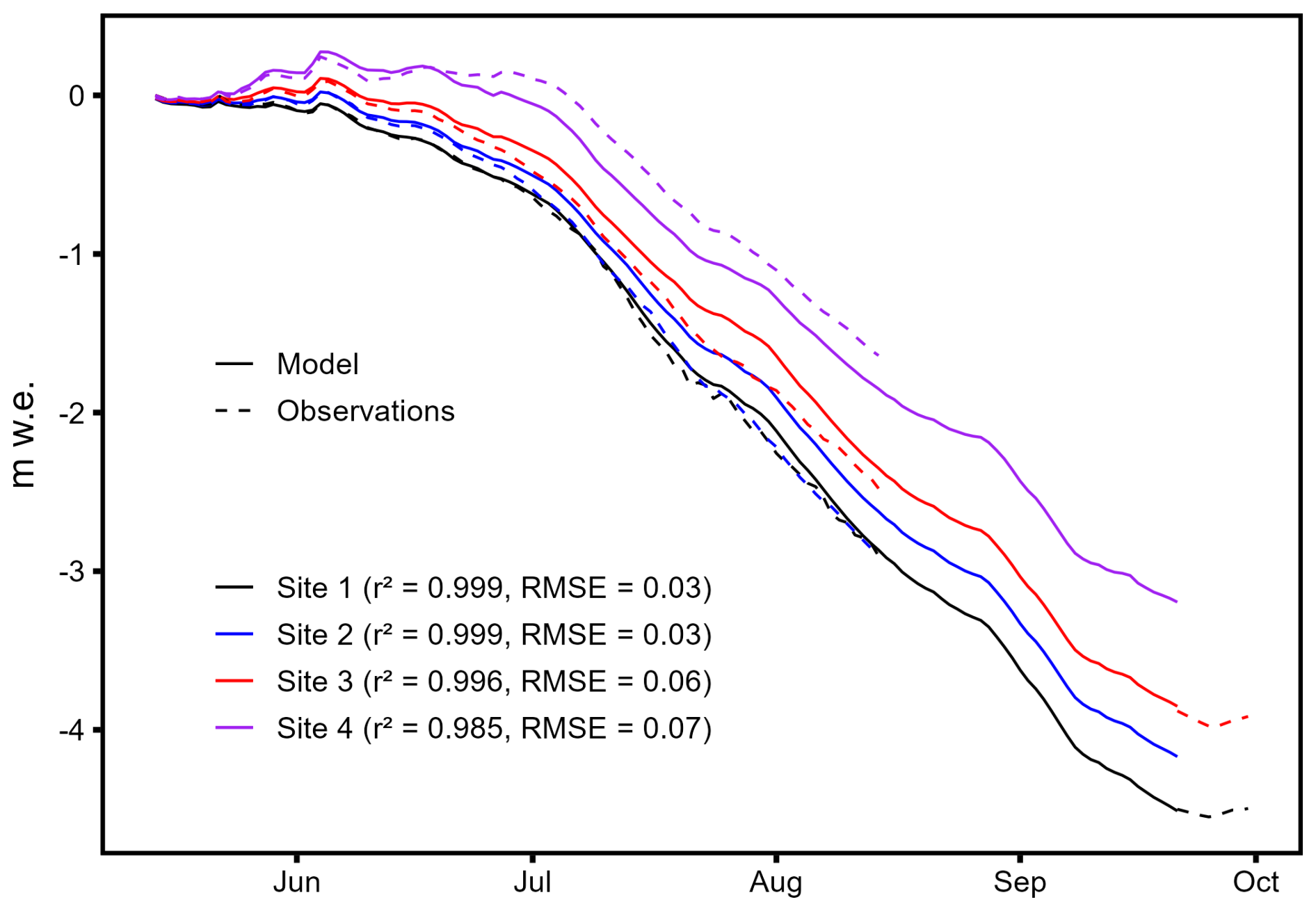
Figure 10 Comparison of the ETI model with the on-glacier linear lapse rate against the observations from the smart stakes. RMSE is in m w.e.

We also compare the total seasonal melt from the models against the manual mass balance stakes and the lidar derived geodetic mass balance (Fig. 11). The selected ETI model using the linear on-glacier lapse rates to predict melt at the independent ablation stakes performed well (r²=0.63; RMSE 0.33 m), but we observed better results (r²=0.82; RMSE = 0.23 m) with the ETI model using the linear on-glacier lapse to simulate mass loss observed in the geodetic (Lidar) data at the same stake locations (Fig. 11).

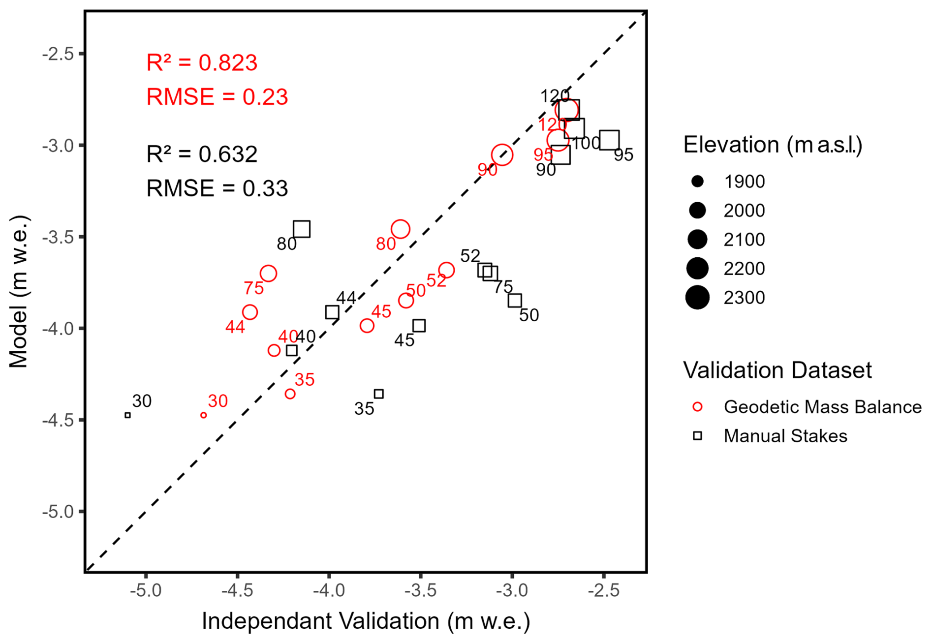
Figure 11 Scatterplot of the measured and modelled summer mass balance at the independent manual stake locations. Black squares represent the manual mass balance data collected by the WGMS, and the model and from the spatial models (m w.e.). Manual stakes were visited on 19 April and 21 September 2024; geodetic mass balance uses the 11 May and 12 October lidar data; and the model is run from 14 May to 21 September. The point labels are the stake names from Table 2, and the R² and RMSE (in m w.e.) are shown in the plot. The dashed line is a 1:1 line. The point size scales to elevation.

Summary raster data from the daily ETI model using the on-glacier linear lapse rate reveal expected spatial variability in drivers of surface melt (Fig. 12). The total PDD values from 14 May to 21 September show an average daily lapse rate on the glacier of −3.06 °C km⁻¹. The minimum, median, and maximum total PDD on the glacier are 765, 927, and 1016 °C (Fig. 12). The average TF_MLR and SRF_MLR coefficients (Table 3) are applied to the daily snow masks, which essentially reflect the number of snow-covered days in the model. The average SR shows shaded portions of the upper glacier to the southwest and shows that the mid glacier plateau has greater SR values than the toe (Fig. 12). The total melt volume from Place Glacier between 14 May and 21 September 2024, was modelled at 12.1×10⁶ m³ of water; the lidar-derived total melt was 11.2×10⁶ m³ of water. Using a normal lapse rate of −6.5 °C km⁻¹ with the ECCC weather station, the ETI model estimated the total melt as 8.04×10⁶ m³ of water. The average modelled pixel level melt is −4.29 m w.e. (Fig. 12) whereas the average glacier-wide modelled mass balance is −4.33 m w.e. (melt volume divided by glacier area).

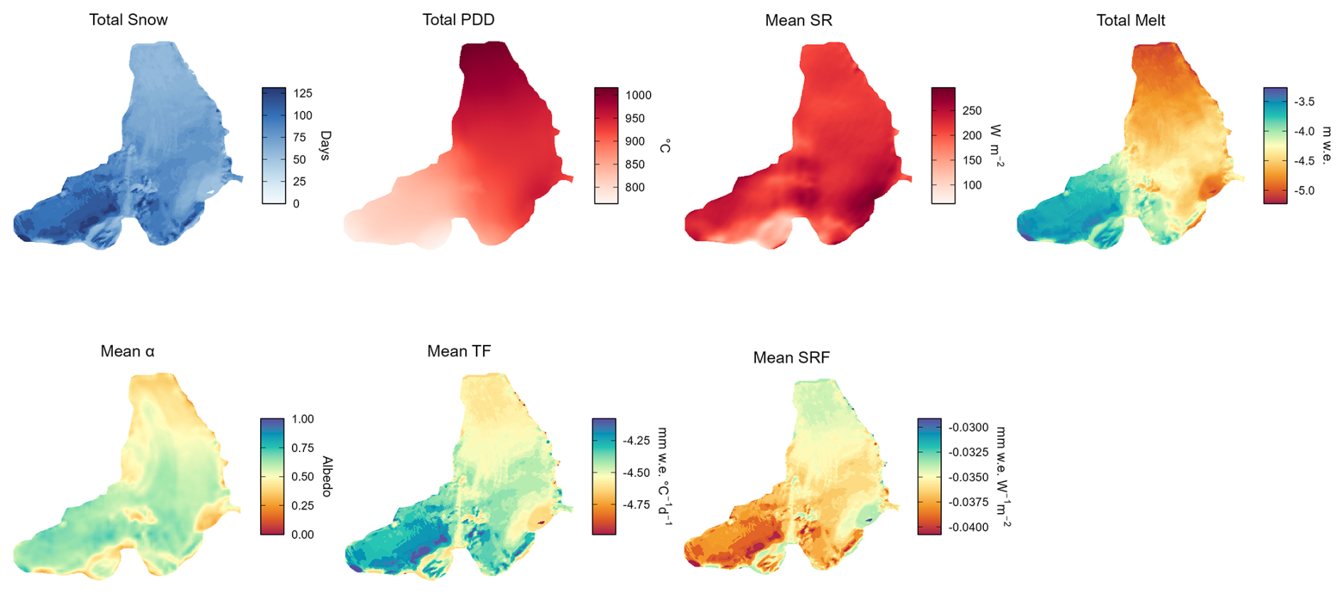
Figure 12 Map of Place Glacier showing ETI model results from 14 May to 21 September 2024: The total snow days; the total positive degree days (PDD) using the on-glacier linear lapse rate; the mean incoming shortwave radiation (SR); the total melt from the ETI model with on-glacier linear lapse rate; the mean albedo (α); the mean temperature melt factor (TF_MLR); and the mean shortwave radiation melt factor (SRF_MLR).

5.7 Event monitoring

The melt model daily change rates are primarily negative during the ablation season, with an overall average daily melt of −38, −36, −34, and −30 mm w.e. d⁻¹ (Fig. 13A). The majority of the melting occurred in July, August, and September when air temperatures exceeded 10 °C. The average [maximum] melt rates for Sites 1–4 are −63 [−77], −60 [−73], −57 [−72], and −51 [−71] mm w.e. d⁻¹ at Sites 1–4, respectively (Fig. 13A).

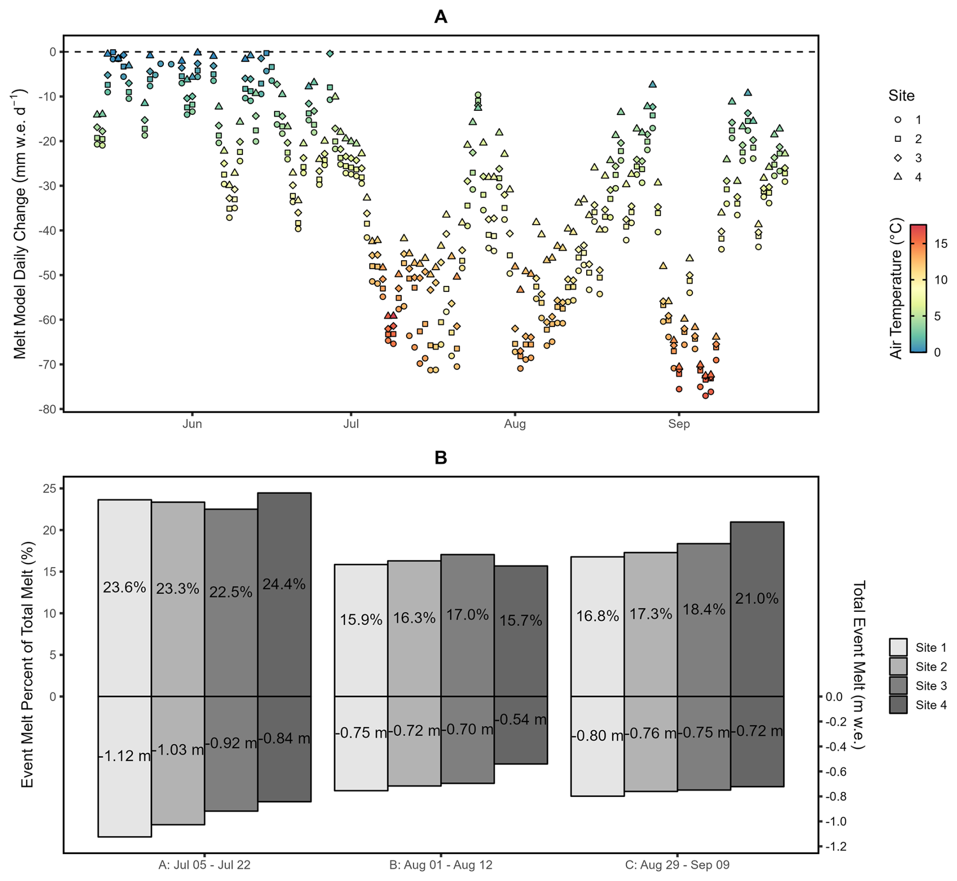
Figure 13 (A) Melt-model daily changes (mm w.e. d⁻¹) colored by average daily air temperature (°C); (B) Percent of seasonal melt for each station that occurred during melt events (A) 5–22 July 2024; (B) 1–12 August 2024; and (C) 29 August–9 September 2024.

We observe three heat events where average air temperatures exceeded 10 °C at all sites (Fig. 13B). The first event (Event A) occurred 5–22 July 2024, Event B took place 1–12 August 2024, and Event C happened 29 August–9 September 2024. We compare the total melt from these three events (39 d, 30 % of total melt period) to the total melt of the season (130 d). These three events account for, on average, 23.5 %, 16.2 %, and 18.3 % of total summer melt, respectively. These events are responsible for over half of the total melt at Sites 1–3 (56.3 %, 56.9 %, 57.9 %, respectively) and 61.1 % of the total melt at Site 4 (Fig. 13B). Event A impacted all sites with between −0.84 and −1.12 m w.e. of melt in 17 d (average rate of −5.7 cm d⁻¹); Event B impacted all sites with between −0.54 and −0.75 m w.e. of melt in 11 d (−6.2 cm d⁻¹); and Event C impacted all sites with between −0.72 and −0.80 m w.e. of melt in 11 d (−6.9 cm d⁻¹).

6 Discussion

6.1 Practical considerations

The integration of low-cost sensors, Arduino microcontrollers, and satellite telemetry enabled the collection of melt data during the 2024 ablation season at Place Glacier, British Columbia, Canada. Several practical advantages emerge from near real-time melt data (Cremona et al., 2023; Wickert et al., 2023). For example, automatic data backups, network status dashboards, and data for decision making and modelling (Bevington, 2025). In addition, their inexpensive nature is ideal for deployments on dynamic glacier surfaces where equipment loss is a risk, and to cover a wide range of glacier conditions. Smart stakes are not a substitute for fieldwork. In fact, given the substantial glacier melt observed globally in recent years (Hugonnet et al., 2021), more frequent field visits may be necessary to reset stakes before they melt out – especially near the glacier terminus (e.g. Fig. 5). Smart stakes can operate anywhere with Iridium satellite coverage, though further testing is needed for high-latitude or high-altitude environments, or for long-term deployments.

The number of stakes required per glacier in future applications will depend on the research question, for example: (1) sample many glaciers with a single smart stake near the equilibrium line altitude; (2) achieve complete coverage of the glacier's elevation range; or (3) capture niche glacier surfaces. Based on our observations, the tipping over of the smart stakes arises from a feedback between heating of the aluminum pole and heat transfer to one ice edge along the pole: as the pole melts into the edge more of the pole is in contract with the ice thereby accelerating leaning of the pole. This effect could potentially be mitigated in the future with a longer stake that is drilled deeper in the glacier, or by developing a self-adjusting tripod. Similarly, an inexpensive tiltmeter could be added to the stake to identify tilting.

In future work, multiple dGPS surveys and snow density measurements are recommended, but not essential. Repeat lidar and satellite imagery, however, are not required for smart stake deployment. The repeat lidar was helpful in this study to quantify the melt while the stakes were tipping over, and remote sensing identifies the snow and ice cover. The smart stakes are well suited for glaciers with no repeat lidar and challenging remote sensing conditions (e.g. persistent clouds).

6.2 Event-scale observations

Traditional mass balance data are generally insufficient for melt attribution studies that require a dense time series of melt data (Kaspari et al., 2015). Our smart stake data quantified the glacier response to short-duration melt events. In our study, more than half of the total seasonal melt occurred in only about a third of the ablation season during three discrete heat events (Fig. 13). The heat events are often accompanied by inverted (positive) air temperature lapse rates (Fig. 8), also reported by Ayala et al. (2015). These findings align with Reyes and Kramer (2023), who documented accelerated snowmelt during successive heat wave events in western North America, and with Pelto et al. (2022), who observed melt rates increase during heat waves in the Nooksack Basin, North Cascades. These rich observations allow future investigations of melt attribution from, for example, events such as local wildfires or snow-algae blooms (Bertoncini et al., 2022; Williamson and Menounos, 2021) which can occur on time scales which are much shorter than an ablation season.

An added advantage of capturing melt events in real-time is the opportunity this presents for flood forecasting (Nester et al., 2012). Real-time data assimilation of glacier melt is not currently available from operational monitoring groups in Canada. Government agencies operate weather stations, hydrometric stations, and traditional glacier mass balance programs, but to date, no government agency provides real-time glacier melt data. Such real-time data could provide support early warning flooding, such as the flooding that followed the 2021 heat dome event in western North America (Reyes and Kramer, 2023).

6.3 Contributions to melt

Our empirically-derived temperature melt factors for ice and snow using (Table 3) are similar to those reported in previous studies (Braithwaite and Zhang, 2000; Carenzo et al., 2009; Shea et al., 2009; Wickert et al., 2023). For example, Shea et al. (2009) reported TF_i of −4.69 and TF_s of −2.71 mm w.e. °C⁻¹ d⁻¹ for Place Glacier, whereas Wickert et al. (2023) found a range of melt factors from −3.9 to −10.3 mm w.e. °C⁻¹ d⁻¹ across multiple sites from Antarctica to Alaska. Bidlake et al. (2010) noted melt factors for South Cascade Glacier of −3.9 mm w.e. °C⁻¹ d⁻¹ for snow and −5.6 mm w.e. °C⁻¹ d⁻¹ for ice. On Mount Baker in the North Cascades, Pelto et al. (2022) reported −3.5 mm w.e. °C⁻¹ d⁻¹ for snow and −5.3 mm w.e. °C⁻¹ d⁻¹ for ice, and that these rose during heat waves to −4.3 and −6.7 mm w.e. °C⁻¹ d⁻¹, respectively.

Using the ETI model, the respective contributions to the glacier volume changes from the air temperature, shortwave radiation, and accumulation components of Eq. (2) are: $-\mathrm{11}\times {\mathrm{10}}^{\mathrm{6}}$, $-\mathrm{1.8}\times {\mathrm{10}}^{\mathrm{6}}$, and $+\mathrm{0.7}\times {\mathrm{10}}^{\mathrm{6}}$ m³, for a total volume change of $-\mathrm{12.1}\times {\mathrm{10}}^{\mathrm{6}}$ m³. The shortwave component represents, on average, 20.4 % of the daily melt (Fig. S10). These results, however, do not consider the full energy balance due to limited input data, and the covariance between air temperature and incoming shortwave radiation does not allow a proper melt partitioning (Kinnard et al., 2022).

The variability of melt across the glacier highlights the importance of local factors. We observed non-linear and inverted lapse rates across the glacier, with Sites 1 and 2 near the toe experiencing a cooler microclimate than would be expected from a linear lapse rate (Fig. 8). These patterns would not be captured by applying a single lapse rate to an off-glacier station. The off-glacier weather station in the glacier forefield is warmer than the on-glacier sites, particularly in summer, even though it is 23 m higher in elevation than Site 1. These differences may be explained by the topography of the basin and katabatic wind flows (Ayala et al., 2015; Munro and Marosz-Wantuch, 2009). This spatial variability in air temperature regimes underscores the importance of distributed temperature observations across glaciers for accurate melt modelling. Using a normal lapse rate of −6.5 °C km⁻¹ with the ECCC weather station, the ETI model estimated the total melt as 8.04×10⁶ m³ of water (33.5 % less melt than the ETI model with the on-glacier linear lapse rate). A possible improvement would be to include non-adiabatic influences including the distance along the glacier and proximity to the ice margins into a distributed melt model (Ayala et al., 2015; Greuell and Böhm, 1998). The observed variability in the cumulative melt plots likely indicate non-stable melt factors throughout the season and highlight the need for energy balance approaches in future work (Fig. 9).

The integration of in-situ data with airborne lidar and satellite observations demonstrates the power of multi-scale monitoring approaches (Cremona et al., 2023; Pelto et al., 2019). This hybrid approach creates a more comprehensive picture of glacier melt at different spatial and temporal scales. The validation of smart stake measurements against independent lidar observations showed good agreement (RMSEs of 0.18–0.12 m for Sites 1–3), though Site 4's higher RMSE (0.55 m) highlights the importance of considering installation conditions, local topography and ice velocity when interpreting point measurements (Beedle et al., 2014). A likely explanation of the poor model performance at Site 4 is that the stake was only drilled into the snow over the ice and may have settled over time.

6.4 Limitations of the study

Smart stakes. We could not correct the diurnal fluctuation in the ultrasonic data caused by the solar heating of the sensor (Fig. S3). Correcting this bias requires the raw time-of-flight data, which the sensor does not record. The sensor, however, does have the ability to use an external temperature sensor to correct the speed of sound, which we will implement in the future. The fieldwork protocol of continuing the timeseries after the stakes tipped over (e.g. Fig. 7) is a potential source of error. Even though this study contributes notable advancements for glacier monitoring, snow and ice density data is still lacking, particularly over time. Future development of the smart stakes is discussed in the Supplement.

Temperature-index modelling. While the temperature-index and enhanced temperature-index models offer a practical and efficient approach to estimating melt based on air temperature and shortwave radiation, they oversimplify the underlying physical processes of energy exchange and ice dynamics (Hock, 2003; Kinnard et al., 2022). Moreover, they assume a fixed relationship between temperature and melt (via the melt factors), yet this relationship varies with other factors like albedo, cloud cover, and elevation, leading to inaccurate melt estimates over space and time (Landmann et al., 2021; Walter et al., 2005; Wickert et al., 2023). Surface mass balance stakes, automatic or manual, do not account for the horizontal and vertical components of glacier dynamics (Beedle et al., 2014).

Air temperature. We did not adjust air temperature values based on their height above the ice. The smart stakes were installed 8/9 May, and they melted out to about ∼3 m above the ice on 16 July, and were redrilled to ∼1 m. They tipped over in August and were re-drilled on again 21 September. The air temperature sensors remained at the same position on the stakes (at the top), and as such changed their relative height above the glacier surface as the season progressed. As the sensors were between 1 and 3 m above the surface of the glacier for the duration of the season, they remain within the katabatic layer of ∼5 m as found in Ayala et al. (2015).

Remote sensing. The snow and ice mapping from the combined HLS and Planet dataset omits many critical components. The 0.4 threshold to map snow and ice does not account for glacier firn and is not a scalable method to other glaciers. Further, it does not account for other land cover units within the glacier polygon: e.g. nunataks, ice marginal bedrock, water, and other non-glaciated terrain. This is most notable in the comparison of the melt model and the lidar geodetic mass balance where the model over-melts on non-glacier terrain (Fig. S9).

Manual mass balance data. The mass balance reported by the WGMS from manual ablation stakes has several limitations. Typically, the glacier is visited twice per year – once in spring and once in autumn. During the spring, readings of the previous years' stake are not possible (buried), which means that any melt occurring after the late September visit is not captured within the proper hydrological year. Instead, this late-season melt is attributed to the following year. Furthermore, there is a discrepancy in the measurement periods for all the input datasets. NRCan visited the manual stakes on 19 April and 21 September 2024. Whereas we installed the smart stakes on 8 May 2024, which had different end dates depending on their respective performances (Fig. 7). The 2024 lidar flights were from 11 May to 12 October. We ran the melt models from 14 May to 21 September 2024. Using 14 May as the beginning allowed for any initial settling of the smart stakes to occur. This discrepancy in measurement periods could explain a portion the higher performance of the model against the geodetic mass balance (R²=0.82), which has similar dates to the smart stakes, compared to the performance against the manual stakes (R²=0.63), which has an extra month of data in the spring.

7 Conclusions

We developed and tested inexpensive sensors (smart stakes) to monitor glacier melt using satellite communication. Smart stakes enable near real-time, high-temporal resolution ablation measurements critical for the current and future needs of glacier monitoring, flood forecasting, and hydrological modelling (Landmann et al., 2021).

The smart stake network at Place Glacier successfully captured high-resolution melt and meteorological data throughout most of the 2024 ablation season. While Sites 1 and 3 operated without issues, intermittent communication, and sensor failures at Sites 2 and 4 highlighted challenges associated with remote monitoring in harsh environments with low-cost equipment. Despite these setbacks, the data recorded on local storage allowed for a nearly complete seasonal analysis. The MB7374 ultrasonic sensors performed well though they were susceptible to solar heating effects. The satellite-derived snow cover complemented in-situ measurements. Smart stakes present a notable improvement in temporal resolution over traditional mass balance stakes.

The smart stakes also present a complimentary dataset to on-glacier AWS because of the low-cost and ease of installation. The gains over a single weather station from the increased spatial sampling include: (1) quantifying the spatial distribution of melt and melt factors over diverse glacier facies (e.g. debris covered ice, dirty ice, steep slopes, or shaded regions), and (2) a quantification of the spatial distribution of air temperature beyond a single point. These allow for the calibration of the ETI model driven by smart stake data and spatial data. The smart stakes were tested in a data rich environment; however, they are suitable for any glacier and would provide important data at a low-cost for regions without repeat high resolution DEMs and in regions with poor optical satellite imagery.

Moving forward, refinements to the instrumentation, such as improved temperature compensation for ultrasonic sensors and additional redundancy in satellite communication, could enhance data reliability. These findings emphasize the importance of continuous monitoring and improved modelling approaches to better understand the impact of climate variability on glacier melt processes and the downstream hydrological implications.