
the Creative Commons Attribution 4.0 License.
the Creative Commons Attribution 4.0 License.
Lake Ice Thickness retrieval using TanDEM-X immediate interferometry
Peilin Chen

Grant Gunn
Sukhdip Kharoud
Knowledge of Lake Ice Thickness (LIT) is essential for understanding the cryosphere and monitoring current climate change impacts. However, accurately retrieving LIT at the desired spatial-temporal scale remains a challenge, as many lakes are in remote regions and LIT is a logistically expensive parameter to measure. Interferometric synthetic aperture radar (InSAR) provides a novel approach to estimating ice thickness by measuring surface deformations at high resolution. This study used TanDEM-X pursuit mode that offers minimal temporal decorrelation to maintain high coherence for accurate LIT retrieval in thermokarst lakes in Northern Alaska during the 2014–2015 winter season. The InSAR-derived LIT was validated against simulations from the Canadian Lake Ice Model (CLIMo), supported by in-situ snow and ice measurements. Results show consistent ice growth patterns and an RMSE of 0.08–0.26 m, demonstrating that the proposed method captures LIT evolution with reasonable agreement with CLIMo estimates. By employing an immediate interferometric approach, the present study maintains sufficient coherence to isolate and highlight the influence of volume scattering, which shifts the phase center away from the ice-water interface, and is the main factor limiting the accuracy of the LIT retrieval. These findings provide new insights into the technology of InSAR-derived LIT and suggest that SAR missions operating at longer wavelengths, such as NISAR and TanDEM-L, hold significant potential for improving retrieval accuracy by enhancing penetration and reducing sensitivity to internal scattering within the ice volume.
- Article
(8489 KB) - Full-text XML
- BibTeX
- EndNote
Lake ice thickness (LIT) is a crucial parameter for cryosphere studies and climate change monitoring (Brown and Duguay, 2010). Lake ice supports habitable lake ecosystems (Hampton et al., 2017; Ozersky et al., 2025), reacts to climate variability (Brown and Duguay, 2010), and has a socioeconomic impact on nearby communities (Perrin et al., 2015). The World Meteorological Organization's Global Climate Observation System (GCOS) regards LIT as a critical requirement for climate change monitoring, as the primary drivers for ice development are air temperature and snow depth (World Meteorological Organization, 2022). Consistent monitoring of LIT is logistically costly to conduct manually for many remote lakes, making it difficult to accurately retrieve LIT in Arctic regions at the desired spatial-temporal scale (Murfitt and Duguay, 2021). The decline in manual meteorological observation networks is posing increasing challenges to LIT retrieval by limiting the availability of meteorological forcing data required for ice growth models and reducing in situ observations needed for retrieval validation (Vincent et al., 2012). As a result, there has been increasing interest in the use of remote sensing technologies as a potential solution for addressing the limitations of traditional LIT monitoring networks. Previous studies have demonstrated the potential of Synthetic Aperture Radar (SAR) for estimating lake ice growth and thickness variations indirectly (Duguay and Lafleur, 2003; Wegmüller et al., 2010; Duguay et al., 2015), while recent advances in satellite altimetry have enabled progress toward operational LIT retrieval approaches (Beckers et al., 2017; Mangilli et al., 2022, 2024).
Active microwave remote sensing technologies have shown significant potential for LIT retrieval, including radar altimeters that estimate ice thickness from surface elevation measurements and SAR-based approaches that exploit interferometric phase information to monitor ice growth and thickness variations (Murfitt and Duguay, 2021). Since ice and air have relatively similar dielectric characteristics, SAR signals can pass through the air-ice interface and are reflected at the ice-water layer due to the greater dielectric contrast (Hallikainen, 1977). In the early stages of primary ice formation, the thin, smooth ice layer exhibits backscatter characteristics similar to those of calm water, where specular scattering predominates and results in low backscatter (Duguay et al., 2002; Pietroniro and Leconte, 2005). Roughness at the ice-water interface increases during ice thickening, due to bubbles resting at the interface and to variations in ice thickness caused by snow depth variability on the ice surface, which modulate the conductive heat flux exiting the lake (Brown and Duguay, 2010). Increased surface roughness at the ice-water interface increases diffuse surface scattering, raising backscatter in co-polarized channels and making it the dominant return observed for freshwater ice (Engram et al., 2013b; Gunn et al., 2018). If the ice freezes to the lake bed, backscatter will be reduced because the underlying medium (e.g., gravel, soil, permafrost) absorbs most radar signals (Antonova et al., 2016; Weeks et al., 1981). Furthermore, internal structures within the lake ice, such as methane ebullition bubbles and tubular bubbles, influence the backscatter with double-bounce and single-bounce scattering (Jeffries et al., 1994; Engram et al., 2013a). Depolarizing multiple scattering events can also be caused by a high density of microscopic spherical air bubbles in surface ice types (Murfitt et al., 2024; Gunn et al., 2017). Overall, the dominant source of radar returns from freshwater ice has been observed to originate from the roughness of the ice-water interface; microwave penetration through freshwater ice causes the interferometric phase center to be located near the dominant scattering interface which provide height information at the ice-water interface (Gunn et al., 2018).
Accurate retrieval of LIT from satellite sensors remains challenging because radar signals can be affected by snow cover, ice surface, sediments, and internal structures. Early studies used an approach that indirectly determined LIT by combining detected grounded ice with lake bathymetry data for shallow lakes (Duguay and Lafleur, 2003; Hirose et al., 2008). Later, some studies recommended using a regression model from SAR backscatter. However, retrieval errors with a Root Mean Square Error (RMSE) of 11.7 cm result from the increase in roughness at the ice-water interface being uncorrelated with the growth of lake ice, particularly the quick increase in roughness during early lake ice growth (Murfitt et al., 2018; Gunn et al., 2018). Data costs from in-situ training samples also limit the effectiveness of the regression method. Based on successful experiments using ground-based Frequency-Modulated Continuous-Wave (FMCW) radar on lake ice, it has been found that LIT can be derived by measuring the distance between two power peaks in range, representing the snow/ice and ice/water interfaces (Leconte et al., 2009; Gunn et al., 2015). This has led to increased use of radar altimeters for LIT retrieval on satellites such as CryoSat-2, the Jason series, and Sentinel-6 in recent years (Beckers et al., 2017; Li et al., 2022; Mangilli et al., 2024; Zhang et al., 2026). Radar altimeter-based LIT retrieval over freshwater ice exploits the penetration of microwave signals through the ice column and their interaction with multiple scattering interfaces, where the separation between waveform double peaks (or a step-like break, depending on altimetry mode) at the ice surface and the ice-water interface can be converted into ice thickness (Beckers et al., 2017; Mangilli et al., 2024). Recent developments in waveform retracking and peak detection algorithms have improved the identification of these scattering interfaces, enabling more accurate and robust LIT retrieval from radar altimetry observations (Li et al., 2022; Mangilli et al., 2022, 2024).
SAR interferometry has significant potential for LIT retrieval because it provides large-scale gridded imaging at meter-scale spatial resolution. While recent developments in fully focused SAR altimetry can achieve sub-meter along-track resolution, conventional radar altimeter observations remain primarily limited to measurements along satellite ground tracks (Li et al., 2022; Mangilli et al., 2024; Zhang et al., 2026). Large numbers of shallow thermokarst lakes and small water bodies in the pan-arctic region require high-resolution observations to perform LIT mapping (Olefeldt et al., 2016). Several studies have proposed using C-band Differential Interferometric Synthetic Aperture Radar (DInSAR) to monitor LIT growth by measuring phase differences across multiple SAR acquisitions (Wakabayashi et al., 2019; Siles et al., 2022; Ferguson and Gunn, 2023). However, the accuracy of LIT retrieval using repeat-pass interferometry can be limited by low coherence, which is caused by temporal decorrelation from the continually evolving ice-water interface during lake ice growth (Siles et al., 2022; Chen and Gunn, 2025). Using satellite sensors with shorter repeat-pass, such as the Radarsat Constellation Mission (RCM) with under-4 d repeat, can reduce temporal decorrelation, but lake ice deformation, such as cracks and ridges, still leads to a decrease in coherence (Ferguson and Gunn, 2023). A potential solution to the temporal decorrelation impact could be to use cross-interferometry, in which two radar sensors map the Earth's surface in the same orbit with an extremely short temporal baseline (28 min for ERS-2 and ENVISAT), thereby reducing temporal decorrelation (Wegmüller et al., 2010). Recently, the TanDEM-X pursuit monostatic mode experiment on Lac Beauséjour demonstrated high coherence on lake ice after the Freeze-up, providing new insights for LIT retrieval using InSAR (van der Sanden et al., 2018). TanDEM-X was originally developed for bistatic SAR interferometry, with its primary scientific objectives including the generation of a global digital elevation model, rather than lake ice thickness retrieval (Rizzoli et al., 2017). Therefore, the TanDEM-X observations used in this study represent a valuable dataset of opportunity for investigating lake ice thickness using data acquired for a different scientific purpose.
In this study, TanDEM-X repeat-pass observations acquired in pursuit mode are used to generate interferometric height models (Zink et al., 2014) of the ice bottom in freshwater lakes on the Alaskan North Slope. Since X-band sensors can also penetrate ice layers and reach the ice-water interface, this study hypothesizes that elevation derived from TanDEM-X acquisitions can retrieve LIT, with detrimental coherence effects eliminated by using data acquired in pursuit mode (Gunn et al., 2015, 2017). Objectives of this study include: (1) to derive LIT using TanDEM-X interferometry; (2) to investigate the spatial-temporal pattern of lake characteristics such as grounded/float ice distributions; and (3) to compare the LIT retrieval with in-situ measurements and simulated ice thickness using the Canadian Lake Ice Model (CLIMo) to determine the viability of this method.
2.1 Study Area
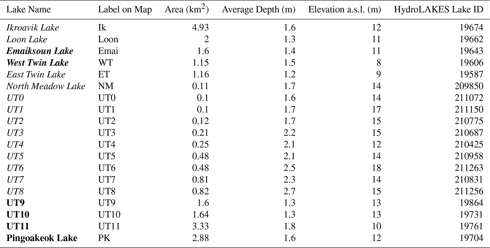
LIT are retrieved for 15 thermokarst lakes in the region surrounding Utqiaġvik (formerly Barrow, Alaska, 156.7674978° W, 71.2946711° N), located on the coast of the Arctic Ocean in a region of continuous permafrost (Table 1). The region is typified by a high density of small, shallow freshwater lakes that are developed thermally through the thawing of ice-rich permafrost, creating a basin that fills with water, forming a talik of thawed soil beneath the lake, with the elongated shape of the lakes oriented in the prevailing wind direction (Carson and Hussey, 1962; Sturm and Liston, 2003). The lakes observed in this study are generally shallow (average depth of 1.87 m), with the maximum and minimum areas of 0.1 and 4.93 km2, respectively. Many lakes in this region are documented to freeze to bed annually (Surdu et al., 2015; Arp et al., 2018) during the prolonged winter, which is an important consideration because of the impact of grounded ice on backscatter and interferograms. Additionally, the lake ice in this area contains numerous bubbles within the ice layer (Engram et al., 2013b).
Table 1Physical properties of lakes included in this study for LIT retrieval. Unnamed lakes are given the label UTn for subsequent sections. Lake Names in bold contain in-situ measurements that can be used for validation, where italicized represents lakes that are within the TanDEM-X footprint of this study which will be used to derive LIT.
The climate surrounding Utqiaġvik is influenced by its proximity to the Arctic Ocean (e.g., the presence or absence of sea ice) and its high latitude. The climatological normal recorded at the Barrow Airport weather station (Station ID: USW00027502), from 1991–2020, is typified by cool, cloudy summers with July average temperatures of 4.6 °C, and cold winters with February average temperatures of −24.9 °C. Precipitation in Utqiaġvik peaks during the summer months (July–September) and averages approximately 157 mm annually. According to climate normals, snowfall occurs in all months, peaking in October at 0.23 m, with an annual accumulation of 0.95 m (Alaska ClimateResearch Center, 2026). From 1949 to 2020, Utqiaġvik has seen an annual increase in air temperature of 4.2 °C; the increase is even more pronounced in winter (+5.6 °C), consistent with general seasonal warming patterns associated with Arctic amplification (Box et al., 2019; Alaska Climate Research Center, 2026).
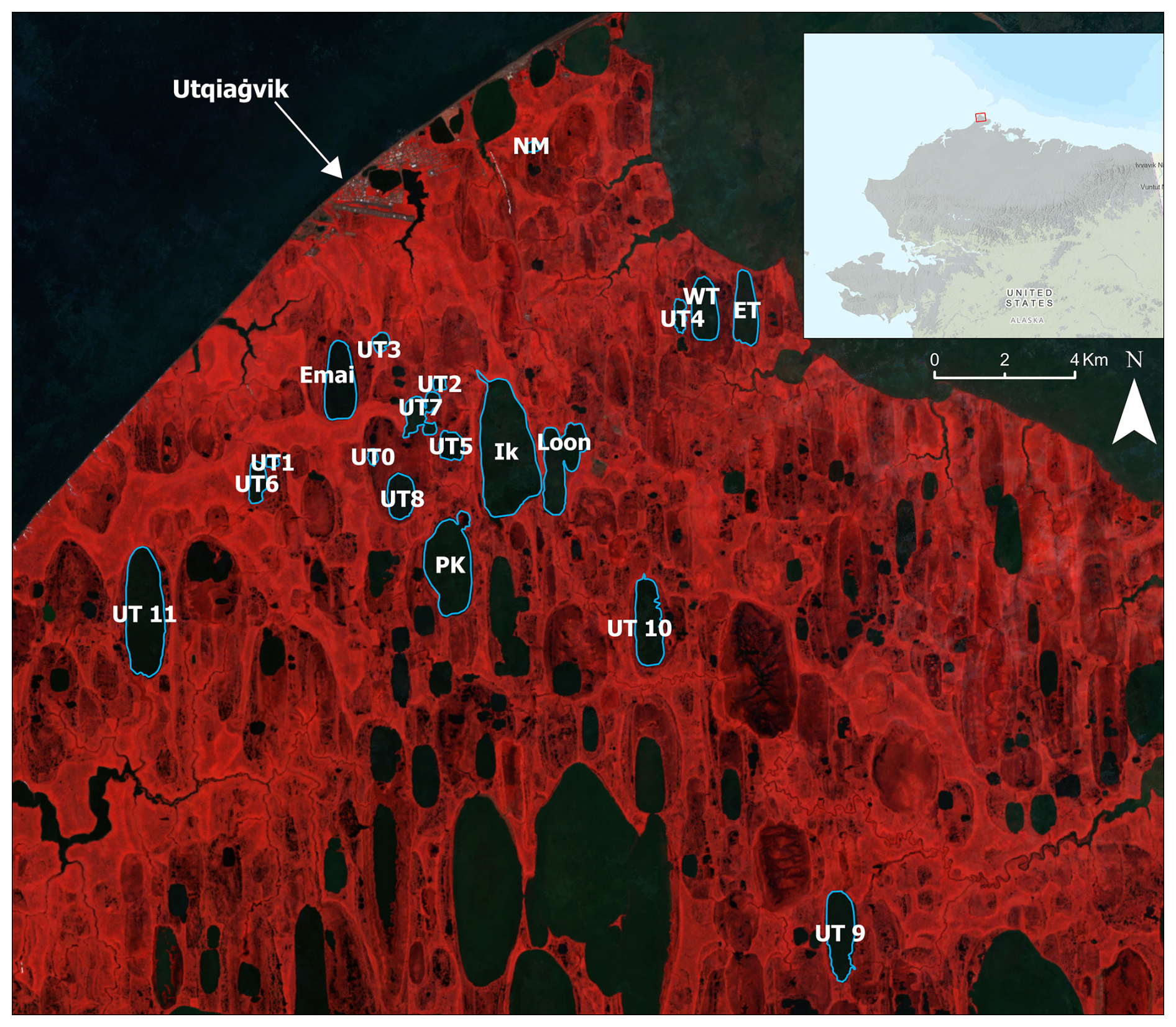
Figure 1Freshwater lakes for ice thickness retrieval surrounding the city of Utqiaġvik within the TanDEM-X acquisitons. Background images is a false colour composite from Landsat 8 derived using the median per-pixel value from an image stack extracted from 2014–2016 during summer months (July–September). The top-right basemap. The base map was designed and developed by Esri | Powered by Esri.
2.2 Methods
The procedure of LIT retrieval and validation is illustrated in the workflow presented in Fig. 2. The workflow can be summarized into three parts: (1) TanDEM-X heights generation; (2) LIT retrieval from individually generated height products; and (3) correction of grounded ice and ice freeboard, followed by accuracy assessment through comparison of in-situ observations and simulated ice thicknesses. The following sections describe each of these steps in detail, including the generation of TanDEM-X height products, the retrieval of LIT, and the subsequent corrections and validation.
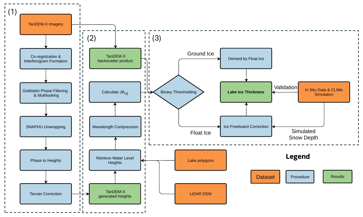
Figure 2Workflow for estimating Lake Ice Thickness using TanDEM-X interferometry framed into 3 parts: (1) Generating TanDEM-X height products; (2) LIT retrieval; and (3) Grounded ice/ice freeboard correction and accuracy assessments.
2.2.1 Data to retrieve LIT
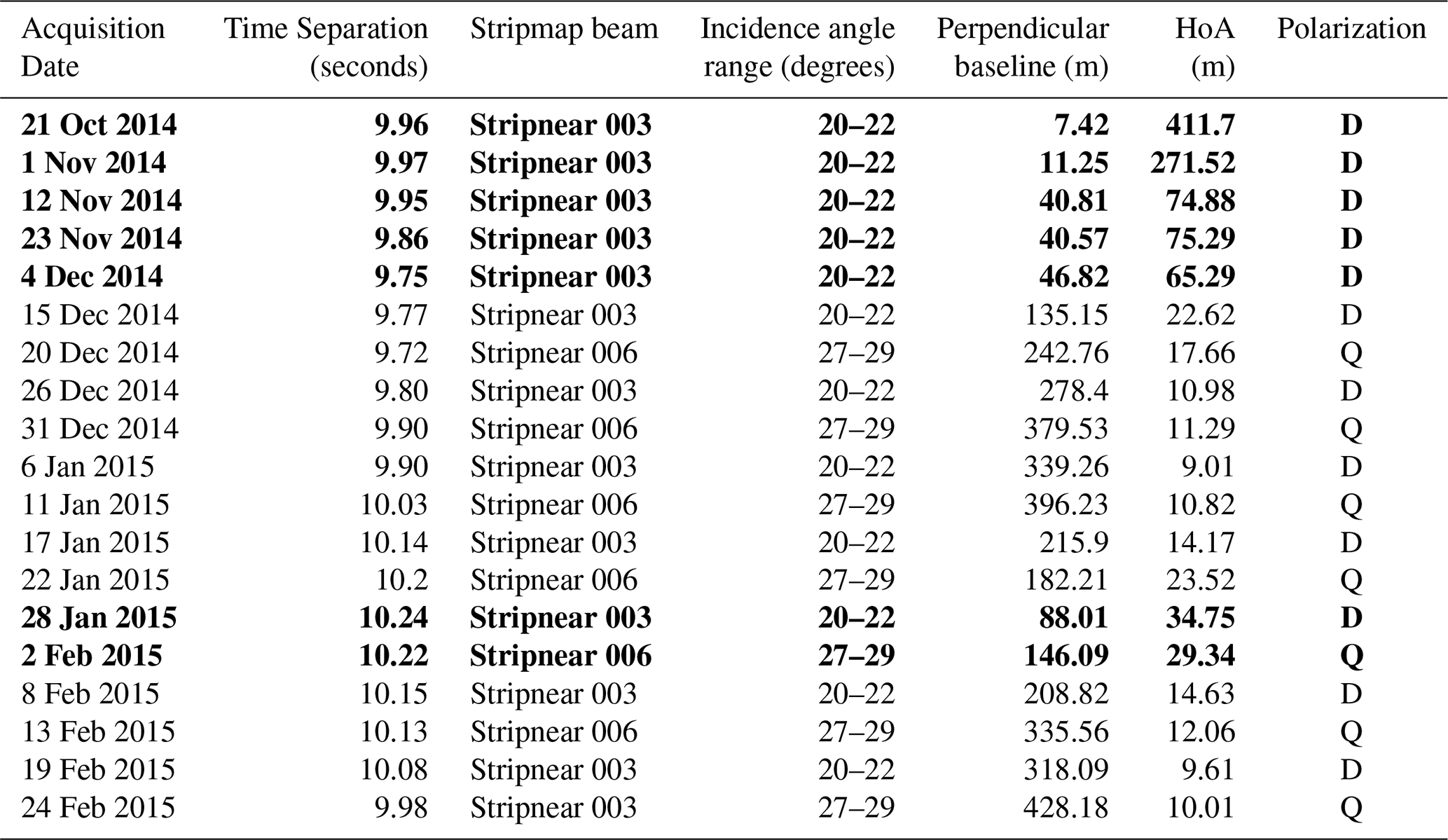
The TanDEM-X mission involves two satellites, TerraSAR-X and TanDEM-X, launched by the German Aerospace Center (DLR) in 2007 and 2010, respectively. A total of 19 observations were acquired by each satellite in StripMap mode with a pursuit monostatic configuration and a short temporal separation of approximately 9–10 s (Table 2). The short repeat pass time results in image pairs over the Alaskan North Slope from October 2014 to February 2015. Stripmap mode acquisition provides fine spatial resolution (approximately 3 m in range and 1–3 m in azimuth). As shown in Table 2, 7 of the 19 TanDEM-X acquisitions are not appropriate for DEM generation due to the Height of Ambiguity (HoA) being too large, resulting from low perpendicular baselines between the two sensors during data acquisition.
For an accurate estimate of LIT retrieval, this study used the North Slope Borough 2018 LiDAR Digital Surface Model (DSM) dataset to retrieve elevation information; the dataset achieved a non-vegetated vertical accuracy of 4 cm (U.S. Geological Survey, 2019). Additionally, the HydroLAKES dataset, providing estimated lake depth information, was used for auxiliary (Dewitz, 2020; Messager et al., 2016).
Table 2Details of TanDEM-X configurations for this study, bolded rows represent image acquisition disqualified for LIT estimation due to large HoA values. Polarization D represents a Dual-Polarized (HH + VV) image, and Q represents a Quad-Polarized image.
2.2.2 TanDEM-X height generation
InSAR is a technology that uses multiple complex SAR images acquired at the same location to retrieve phase correlations and phase differences (Woodhouse, 2006). The phase difference between two radar acquisitions can be interpreted as a topographic displacement by taking the complex conjugate of the primary and secondary images. The interferogram is the sum of multiple phase contributions that:
where φorb refers to orbital and flat earth deviation at different acquisitions, φatm is the noise due to changes of tropospheric water vapour in the atmosphere between two images, and φnoise is caused by changes in the scattering characteristics of targeted objects and by thermal noise. At the same time, φtopo and φdefo were commonly used to retrieve elevation information and measure the surface deformation between two acquisitions (Amani et al., 2021). However, φtopo and φdefo don't only contain the surface information, but it might also be affected by scattering sources from upper layers (Stebler et al., 2002). Because of its sensitivity to scattering from rough surfaces, VV polarization is the preferred method for detecting elevation and surface deformation. To derive surface height from an interferogram, the unwrapped interferometric phase is converted into height. The fundamental relationship links the observed phase difference φ to the height of the target relative to a reference ellipsoid (Woodhouse, 2006; Fletcher et al., 2007). The phase-to-height conversion can be expressed as:
where h is the surface height, λ is the radar wavelength, r is the slant range distance to the target, θ is the incidence angle, and B⟂ is the perpendicular baseline between the two satellite positions. The phase ϕ represents the unwrapped phase. A larger perpendicular baseline decreases the HoA, improving the precision of height generation. HoA represents the height difference generated by 2π phase changes, defined as:
SAR interferometry, which measures the cross-correlation between two co-registered Single Look Complex (SLC) acquisitions using their complex values to generate coherence (a measure frequently used to assess interferogram quality). Additionally, it shows how pixels in the same region have comparable physical and dielectric characteristics. According to Touzi et al. (2002), the coherence (γ) between each pixel of two SLC images, represented by the complex numbers Z1, Z2, can be mathematically expressed as follows:
where i is each sample's number, the operator (*) represents the complex conjugate, and N is the total number of pixel samples. The size of the raster moving window with multiple pixels in azimuth and range determines the value N. Consequently, γ is shown as a complex number in the polar form, the phase difference is represented by the phase angle of γ, and the coherence is measured by the amplitude . The coherence value is a number between 0 and 1. If , then N pixels are fully coherent, showing minimal changes in surface attributes; if , then pixels are uncorrelated. Coherence values under 0.3 are often regarded as worthless for phase unwrapping and displacement measurement (Touzi et al., 2002).
TanDEM-X pursuit image pairs were used to generate Height products for LIT retrieval using the Sentinel Application Platform (SNAP) from the European Space Agency (ESA). Each image acquisition was first masked to the region of interest (Utqiaġvik) to improve processing efficiency, where the polarization band VV was selected for interferogram generation. The TSX and TDX images were then co-registered using 4000 ground control points (GCPs) to align each sub-pixel, reducing geometric errors to an RMS threshold of 0.001. An interferogram, along with the coherence image, was produced with the flat-Earth phase removed, while retaining the topographic phase to preserve height information (Bamler and Hartl, 1998). Goldstein filtering was applied to mitigate phase noise, using a window size of 5 and an adaptive filter exponent of 0.8 (Goldstein and Werner, 1998), followed by multi-looking to reduce remaining interferometric speckles. Phase unwrapping was performed externally using the Statistical-cost Network-flow Algorithm for Phase Unwrapping (SNAPHU) in TOPO statistical-cost mode (Chen and Zebker, 2002). The unwrapped phase was then converted to height, where range-Doppler terrain correction was applied to produce geocoded height products suitable for subsequent LIT retrieval.
2.2.3 LIT retrieval from Interferometry-Derived Heights
To calculate LIT from the TanDEM–X derived Height product, the hydrostatic water level height is extracted from each lake to calculate the height difference (Δheff). Our method builds upon the approach of Wegmüller et al. (2010) while further improving its robustness by accounting for the elevation difference between the lake water surface and shoreline. First, lake boundaries were obtained via high-accuracy digitization based on PlanetScope imagery and LiDAR DSM, and the buffer operation was applied to extract the surrounding terrain adjacent to each lake shoreline using a user-defined buffer distance (20 m). For each lake, we first used the LiDAR DSM to retrieve the median height difference between shoreline topography and water level, defined as hSW. Then, the median of the buffered land pixels from InSAR height products was computed and identified as the shoreline height hshoreline. The water level height was determined by subtracting the hSW from hshoreline. Height of lake ice hlake was extracted for all ice pixels within the lake extent, where Δheff was calculated by subtracting the height of each lake pixel from the water level height through:
LIT retrieval using InSAR requires correction for the refraction of transmitted microwave through the ice from the ice surface to the ice bottom. While the electromagnetic wave travels through ice, its propagation speed decreases relative to its speed in the atmosphere due to the higher dielectric permittivity of ice. The dielectric property of ice can be described by the real part of the dielectric constant ϵ′:
where T refers to the temperature of ice in Celsius; the temperature effect on the dielectric constant is negligible and can be disregarded in this study (Wegmüller et al., 2010). However, lake ice surrounding Utqiaġvik typically contains numerous air bubbles within the ice layer, which alters its effective permittivity (Engram et al., 2013b). The dielectric constant of bubbled ice can be determined by an empirical equation based on its density:
where p is the ice density (g cm−3). Using the density of clear ice (0.917) gives a dielectric constant of 3.17 (Fujita et al., 2000). The density of bubbled lake ice has been observed to be approximately 0.85 g cm−3, along with studies suggesting that using 90 % density from pure ice for bubbled ice also leads to similar values around 0.83 g cm−3 (Zhang et al., 2023; Murfitt et al., 2024). An ice density of 0.85 g cm−3 is therefore used in this study which results in the dielectric constant ϵ′ of bubbled ice around 2.97 (Fujita et al., 2000). Wavelength compression was calculated to correct the wavelength within the ice by using . The equation of wavelength compression can be described as follows, where hice is the corrected ice thickness, and θ referred to as the incidence angle in degrees (Wegmüller et al., 2010):
for an incidence angle of 25°, using the clear ice dielectric constant will result in a compression factor of 0.60, and 0.62 using the bubbled ice dielectric constant.
Additional considerations were applied for bedfast ice pixels that could interfere with the LIT inversion. The location of bedfast ice are masked, as the lakebed transmits the incoming signals through its medium, where phase information at the ice-ground is rarely returned to the sensor (Surdu et al., 2015). Hence, phase information at the bedfast ice is mainly comprised of interferometric noise or scattering objects in the upper layer of the lake ice. Bedfast ice pixels are identified using the backscatter of the VV polarization from the TanDEM-X image, derived by calibrating the SAR imagery to decibels (dB), then applying the Refined Lee filter and multi-looking to reduce speckle. Similar to the study from Engram et al. (2018) for separating bedfast ice and float ice, a statistical test is first adopted to determine whether the SAR backscatter distribution within each lake was bimodal, indicating a mixture of floating and grounded ice. In such cases, a threshold was determined between the two distributions, and all pixels below this threshold were defined as bedfast ice based on Eq. (10). For lakes without a bimodal backscatter distribution, the median backscatter value was evaluated, and if it fell below −11 dB, the entire lake was assumed frozen to the bed. The determination of the threshold is under the assumption that a bimodal backscatter distribution is based on a two-class Gaussian Mixture Model (GMM), where the threshold can be calculated as:
where “Thres” represents the determined threshold, μFloat and μBed represents the mean value of the Float ice and Bedfast ice, and σFloat and σBed are the standard deviations of the two ice types. The thickness of bedfast ice was determined by calculating the growth of floating ice between image acquisitions for each lake and applying that growth to grounded ice pixels that were still floating at earlier image acquisitions.
To correct the buoyant displacement of floating lake ice, an ice-freeboard calculation is applied to find the portion height of floating ice above the hydrostatic water level. The relationship between float ice thickness (T) and ice freeboard (Fi) is expressed as:
where Hs is snow depth, and ρw, ρi, and ρs are the densities of water, ice, and snow, respectively. In this study, densities of 1030 kg m−3 for water, 850 kg m−3 for ice, and 340 kg m−3 for snow were adopted based on field measurements of bubbled lake ice and typical overlying snowpack parameters for the region (Domine et al., 2012; Zhang et al., 2023). Snow depth (Hs) values were obtained from the CLIMo simulations. To assess sensitivity to snow loading, two potential freeboard estimates are generated using snow cover conditions of 25 % and 50 % from CLIMo model outputs presented in Sect. 4.5. Finally, the Fi were added to the original thickness T to retrieve corrected ice thickness values.
2.2.4 The Canadian Lake Ice Model (CLIMo) constrained by In-situ measurements
Lake ice thickness is simulated for a series of mixing depth and snow cover scenarios using the Canadian Lake Ice Model (CLIMo), which is a one-dimensional thermodynamic model that has been utilized for ice phenology, composition (snow ice, clear ice) and thickness simulations for many freshwater studies in both deep and shallow lakes (Duguay et al., 2003; Brown and Duguay, 2011; Morris et al., 2005; Gunn et al., 2015). Also, CLIMo has been extensively applied and validated for shallow thermokarst lakes in northern Alaska and other tundra environments (e.g., Surdu et al., 2014, 2015; Antonova et al., 2016), supporting its use as a regional-scale representation of lake-ice thermodynamic evolution despite inherent uncertainties in the model inputs and simulations. A full description of the model is provided in Ménard et al. (2002); however, the components relevant to ice thickness are provided below.
The surface energy budget in CLIMo is evaluated through:
where F0 is the net heat flux absorbed at the surface, ϵ is the surface emissivity, σ is the Stefan Boltzmann constant, T is the temperature in Kelvin, α is the surface albedo, and Flw, FSW, Flat, and Fsens are the downwelling longwave, shortwave, latent, and sensible heat fluxes in W m−2, respectively.
Once frozen, ice growth at the bottom of the ice (congelation ice) is derived through the difference between the conductive heat flux through the ice column and out of the surface of the fixed mixing layer (in this case, the lake depth), given through:
where hi is the ice thickness, k is the thermal conductivity, z is the vertical coordinate (m), I0 is the fractional shortwave radiation flux that penetrates through the surface, K is the bulk extinction coefficient for penetrating shortwave radiation, and dz is the thickness of the ice layer (Duguay et al., 2003). is the shortwave radiation that penetrates through the bottom of the ice column, which is assumed to be absorbed in the mixed layer and returned to the bottom of the ice. A feature of shallow lakes, however, is that the mixed layer may also be subject to heat flux from the bottom of the lake itself, which is treated in CLIMo with a fixed constant heat flux from the bottom. A fixed heat flux from the lake bottom is a simplification that may introduce uncertainty into the LIT simulations.
CLIMo is run for all lakes where the mixing depth was set to the lake depth value from the HydroLAKES dataset; the mixing layer depth represents the measure of heat storage in the lake. Shallow lakes are well mixed with an isothermal temperature profile during ice-off conditions, and therefore the mixing layer depth equalling the average lake depth provides a good approximation of the lake's temperature gradient prior to freeze-up.
Since the standard CLIMo formula does not explicitly constrain ice thickness growth with lake depth, we introduced a simple geometric condition to describe the transition from floating ice to bottom-freezing ice. When simulated ice thickness reaches the corresponding lake depth, growth of the bottom-freezing ice is set to zero. Consequently, lake ice thickness is only permitted to increase before reaching the local lake depth, with further thickening inhibited once contact with the bottom is established.
CLIMo is forced with weather data collected from a combination of available sources. Air temperature, humidity, precipitation, and wind speed are obtained from the Barrow Airport weather station (Station ID: USW00027502). Cloud cover fraction, a value not commonly observed at automated weather stations, was collected from the National Oceanic and Atmospheric Administration (NOAA) Climate Data Record (CDR), specifically the Pathfinder Atmosphere Extended (PATMOS-X) product, available in the Google Earth Engine repository (Heidinger et al., 2014). Fixed inputs to CLIMo are mixing depth, dry and wet snow densities, and latitude, with dry snow density using the same values (340 kg m−3) as freeboard estimation (Domine et al., 2012). In the absence of field measurements, the empirical-based wet snow density of 450 kg m−3 was applied, which will not significantly change the CLIMo simulation of this study because snow melting is unlikely to occur on the timescale of this study (Rafat et al., 2025). Snowpacks on lakes have been documented as highly variable, considerably more than on land, as a function of the lack of vegetation to serve as catchments and variations in wind fetch from lake to lake that redistribute snow. A common approach to account for snowpack variability is to run CLIMo with several snowfall scenarios, incorporating 0 %, 25 %, 50 %, and 100 % of the snowfall observed at the weather station. The 0 % and 100 % snowfall scenarios represent the expected range of LIT that could be present, with 25 % and 50 % calibrated by comparing snow depth simulations with in situ measurements (Arp et al., 2018). Therefore, CLIMo is run for a total of 75 simulations across 15 lakes and 5 snow-cover scenarios.
There are limited in-situ observations to use as validation for InSAR-derived LIT retrieval. The only available in-situ ice thickness observations are from the Circum Arctic Lake Observation Network (CALON), which aims to measure thicknesses as they approach or reach their maximum (Arp et al., 2018). There were measurements of LIT and snow depth conducted on six of the lakes in this study where lake WT and Emai are within the TanDEM-X footprint, other four lakes are outside the TanDEM-X footprint. LIT were measured on 7 April 2015, well after the last TanDEM-X image pair on 25 February 2015. These in-situ observations are used to calibrate thermodynamic ice simulations from CLImo.
2.2.5 Accuracy Assessment
The interferometric phase reflects the composite response of all scattering sources within the radar penetration depth (Stebler et al., 2002). While the primary contribution usually originates from the ice-water interface, additional scattering from the overlying ice layer shifts the effective phase center upward relative to the true interface. Consequently, most lake pixels for bubbled ice will underestimate LIT values. However, this phase center displacement exhibits spatial variability; regions with more transparent ice or fewer inclusions allow deeper radar penetration, yielding a phase center closer to the ice-water interface. Consequently, the InSAR-derived LIT distribution within each lake should be constrained by an upper bound on actual ice thickness, with the maximum value corresponding to pixels least affected by volume scattering and phase center bias. Based on this physical interpretation, LIT is retrieved from the 99.7th percentile (3 standard deviations from the normal distribution) of each lake's LIT distribution to estimate lake-scale ice thickness, providing a robust upper-bound approximation while minimizing sensitivity to noise and isolated outliers.
To evaluate the LIT accuracy, TanDEM-X-derived LITs are aggregated to the lake scale by computing the thickness at the 99.7th percentile for each lake at each image acquisition. Then, retrieved values are compared with the corresponding CLIMo-simulated ice thickness for the same lakes and dates. Accuracy assessment is performed for each lake across all temporal acquisitions using the Root Mean Square Error (RMSE), Mean Absolute Error (MAE), and Mean Bias Error (MBE) (Eqs. 8–10, respectively). RMSE and MAE measure the overall magnitude of discrepancies between the satellite-derived LIT and modelled LIT, and MBE quantifies systematic over- or underestimation across lakes and dates. Three accuracy assessment metrics can be computed as:
where Pi and Oi represent the median InSAR-derived thickness and CLIMo-simulated thickness for each image acquisition i at a given lake, and n is the total number of valid TanDEM-X image acquisitions (12 for this study). Negative MBE demonstrates underestimation of LIT, and positive MBE represents overestimation. It should be noted that the comparison between CLIMo-simulated and TanDEM-X-derived ice thickness demonstrates the potential of the InSAR-based approach to retrieve lake ice thickness in this case study; however, the reported RMSE and other statistical metrics quantify the differences between the two estimates and should not be interpreted as direct measures of the true error of the TanDEM-X-derived ice thickness relative to ground truth.
To constrain the snow cover scenarios for CLIMo simulations, field measurements of snow depth observation from 7 April 2015, were compared with the simulated snow conditions. Field observations from six lakes indicated snow depths between 19.65 and 32.05 cm, respectively (Table 3). These values fall within the range of the CLIMo snowcover scenario, corresponding to 25 % to 50 % of the terrestrial snow depth used as atmospheric forcing in the model. This aligns with typical wind redistribution processes in Arctic Lake environments. Consequently, the CLIMo simulation scenarios employing 25 % and 50 % snow cover proportions were selected as the most realistic comparison scenarios for validating InSAR-derived thickness. Moreover, the in-situ ice thickness measurements (127–152 cm; Table 3) are consistent with the CLIMo simulations under both the 25 % and 50 % snow-cover scenarios, which predict average ice thicknesses of 140 and 131 cm, respectively, supporting the suitability of these scenarios and demonstrating the potential of CLIMo to provide a physically consistent benchmark for assessing the accuracy of the InSAR-derived LIT.
Table 3Snow Depth and Ice Thickness on 7 April 2015, from In-situ measurements and CLIMo simulations.
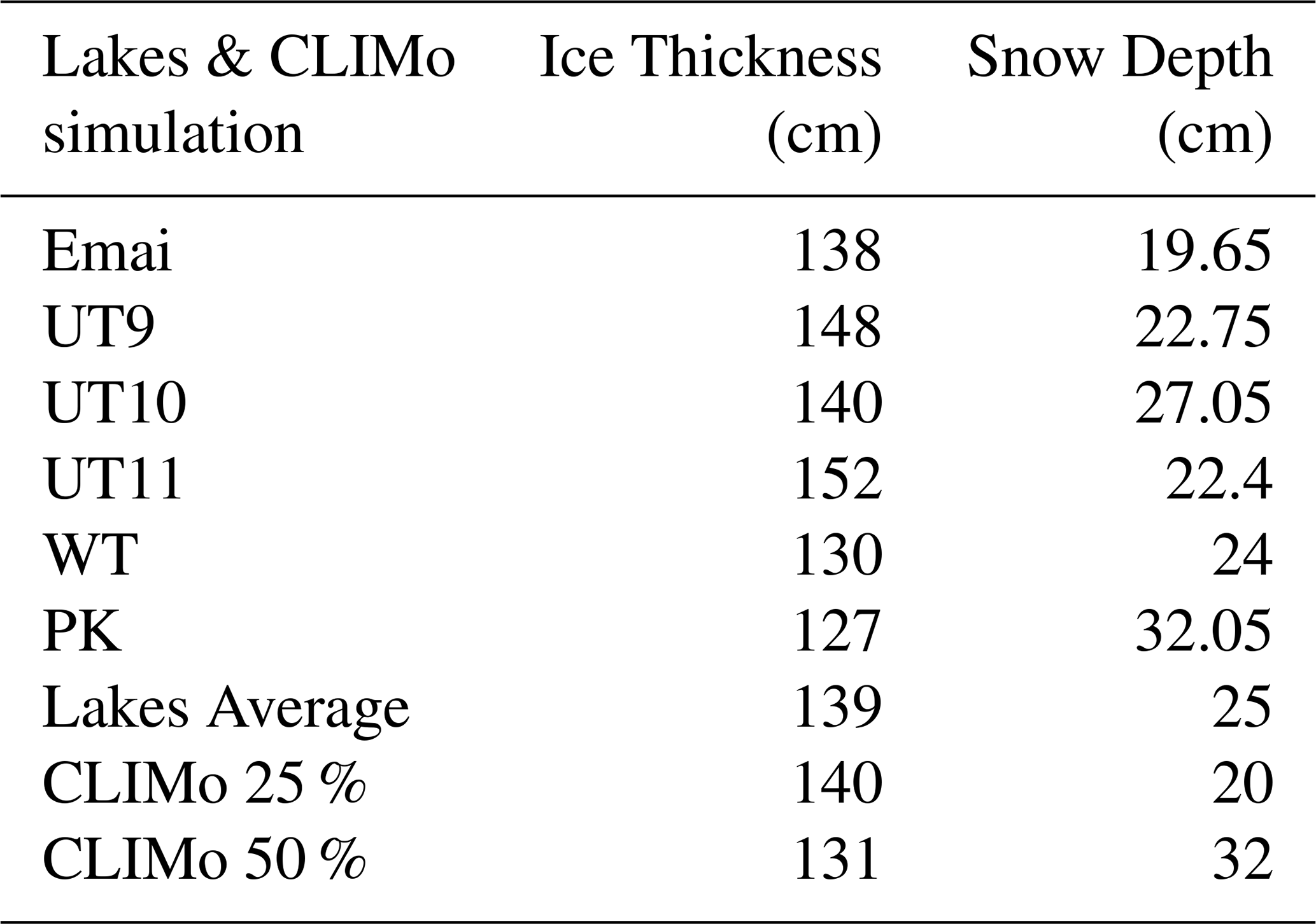
Figure 3 illustrates the observed backscatter and interferometric coherence for lakes in the study region, showing that high coherence values are present for all lakes throughout the winter from the TanDEM-X image pairs, with average values exceeding the 0.3 threshold for viable interferometric analysis (Table 4). For example, the median coherence observed at the Ikroavik Lake is estimated to be around 0.95 on 22 January 2015 (Table 4). After the ice is frozen to the lake bed, the coherence value can be impacted. In the grounded regions, the coherence values are lower than those of floating ice (Fig. 3), with notable differences for all lakes with grounded ice reported in Table 4, especially for late-winter acquisitions.
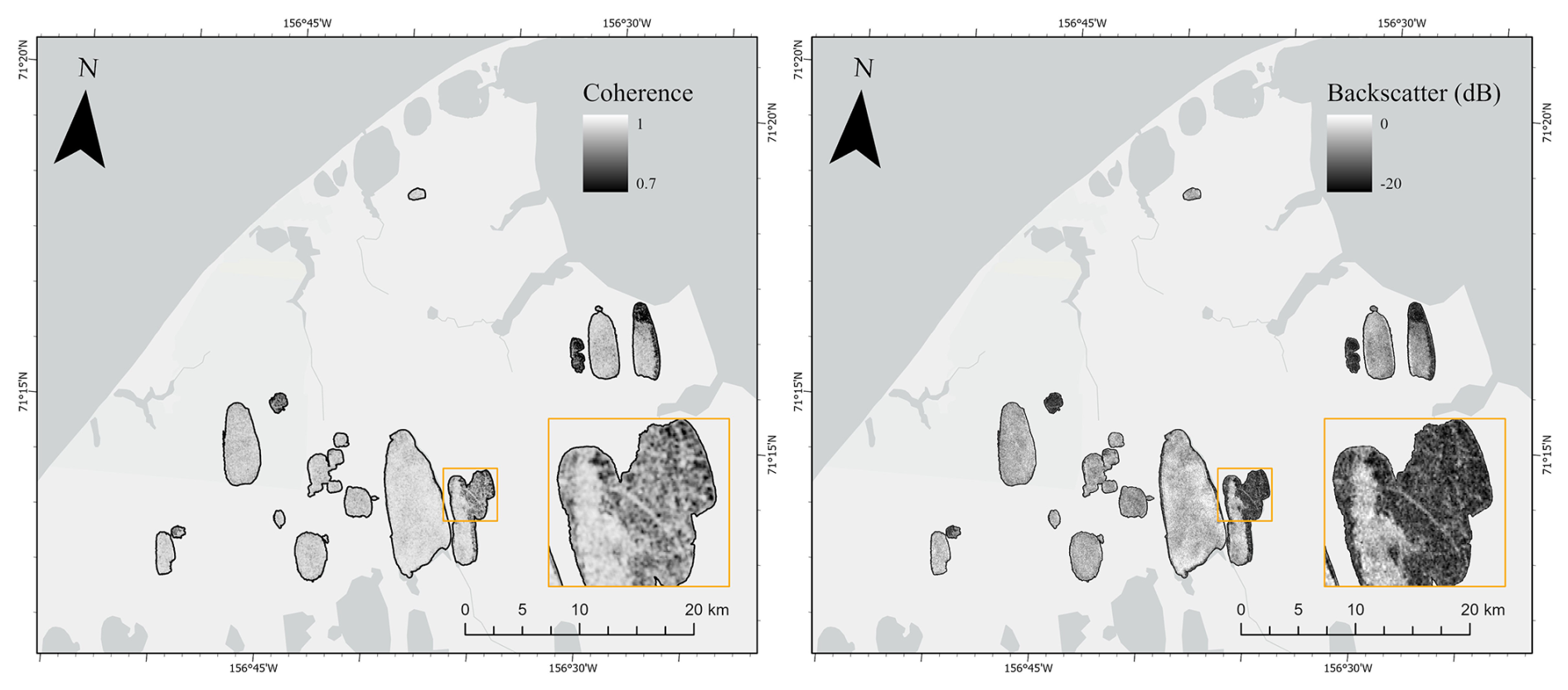
Figure 3Coherence (left) and backscatter (right) observed at acquisition 22 January 2015, grounded Ice with darker pixel values also demonstrated lower coherence.
Table 4Median Interferometric coherence for each lake and each image acquisition, where partially grounded lake ice is in italic and the bold represents the lake fully frozen to bed.
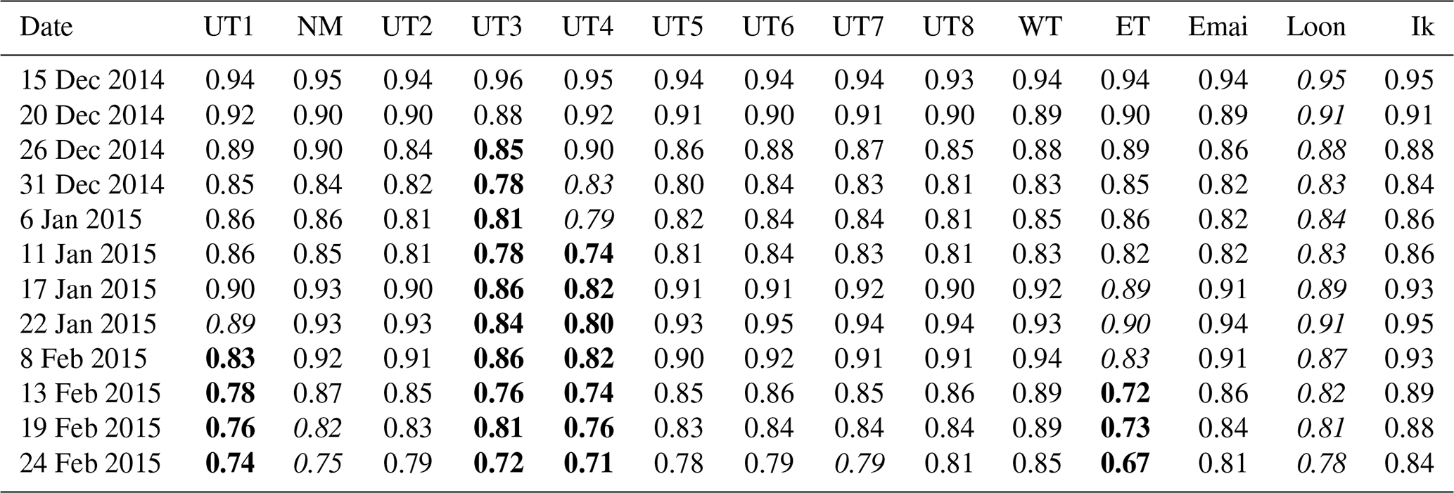
Figure 4 presents the TanDEM-X-derived unwrapped phase and elevation maps for the study area. In both products, the spatial extent of the lakes can be visually distinguished from the surrounding terrain, with lake surfaces visually shown as smooth regions in the unwrapped phase map and as slightly lower elevations in the elevation map. Notably, the elevation within each lake is consistently lower than the elevations along the adjacent lakeshore. Observations across all lakes in the study region provide evidence that the TanDEM-X signal penetrates the lake ice and reflects from within the ice volume or the ice–water interface, supporting the use of TanDEM-X elevation anomalies for LIT retrieval.
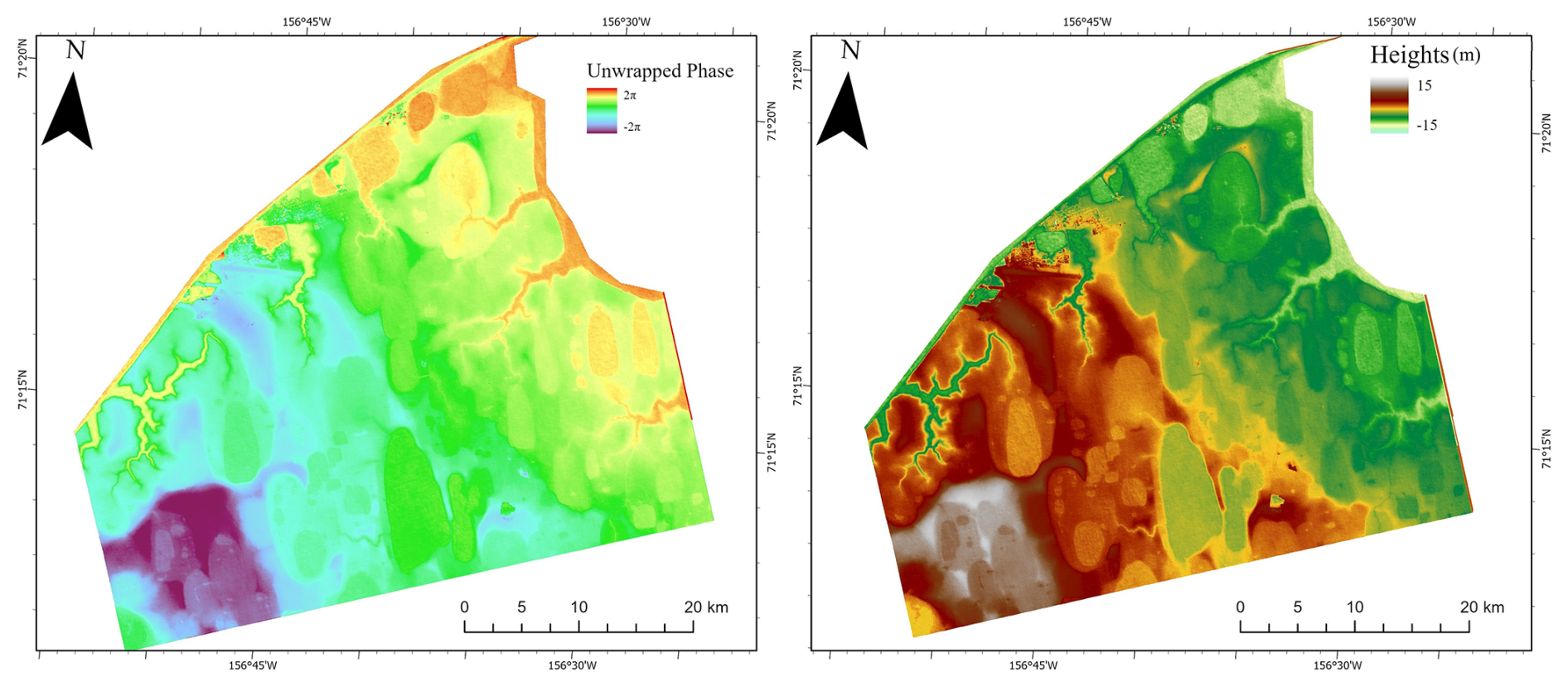
Figure 4Unwrapped Phase (left) and the conversion to height product (right) processed by SNAP for the region surrounding Utqiagvik, Alaska. TanDEM-X observations were acquired on 15 December 2014.
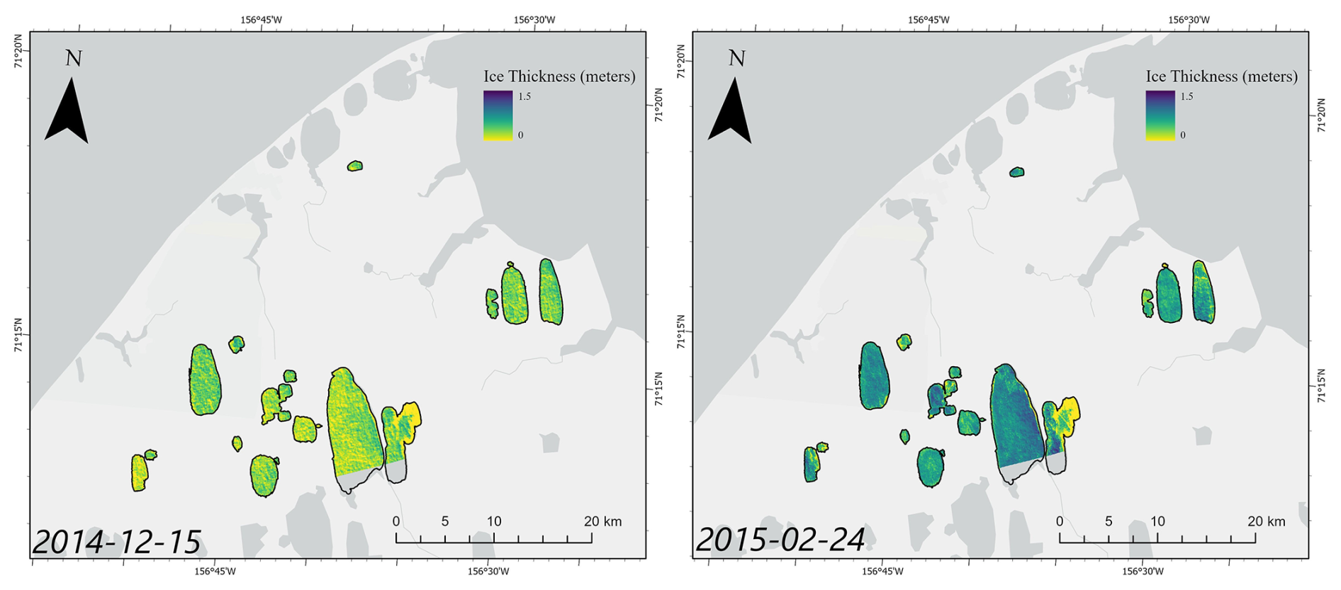
Figure 5Maps of estimated LIT at image acquisition of 15 December 2014 (left) and 24 February 2015 (right).
Figure 5 displays the spatial distribution of InSAR-derived LIT within the 2014–2015 winter periods – early winter (15 December 2014) and late winter (24 February 2015). The comparison clearly shows continuous ice thickening in the study area, with an overall increase in LIT between the two observations. During early winter, most lakes exhibited thin and uniformly distributed ice cover. By late winter, the ice had not only thickened but also displayed more pronounced heterogeneity. Given the relatively small size of the lakes studied, ice growth does not exhibit the spatial variability seen in larger lakes (Siles et al., 2022). Consequently, the depth of the lakes themselves is the primary factor determining variations in ice thickness. Notably, Loon Lake exhibited limited ice thickness, indicating ice-bed fixation where the ice layer has contacted the lake bottom, hindering further growth of the bottom ice. In contrast, deep lakes exhibited a consistent thickening pattern and more pronounced spatial gradients, reflecting ongoing freeze-up under floating-ice conditions.
There are several Quad-polarization TanDEM-X acquisitions, which allow us for polarimetric decomposition to understand the scattering mechanisms observed over lake ice, presented in Fig. 6 for early (20 December 2014) and late (24 February 2015) winter observations. Regions of surface bounce and volume scatter are presented as blue and green, respectively. Although surface bounce dominates, the contribution of volume scattering is considerable, especially during late winter (24 February 2015), where the contribution of volume scattering increases in the West Twin Lake and Ikroavik Lake compared to early winter (20 December 2014). This observed increase of volume scattering correlated with increased bubble inclusions and heterogeneity within the ice volume during ice growth, or surface ice formation (McRae-Pharo, 2025).
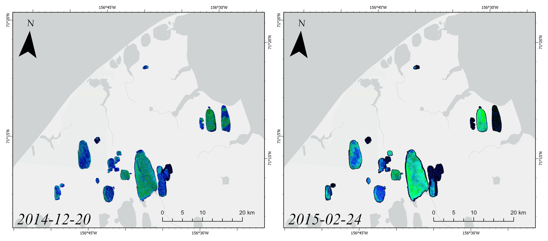
Figure 6RGB composite (Red: Double-bounce, Green: Volume scattering, Blue: Surface-Bounce) of Freeman-Durden decomposition result between 20 December 2014 (left) and 24 February 2015 (right).
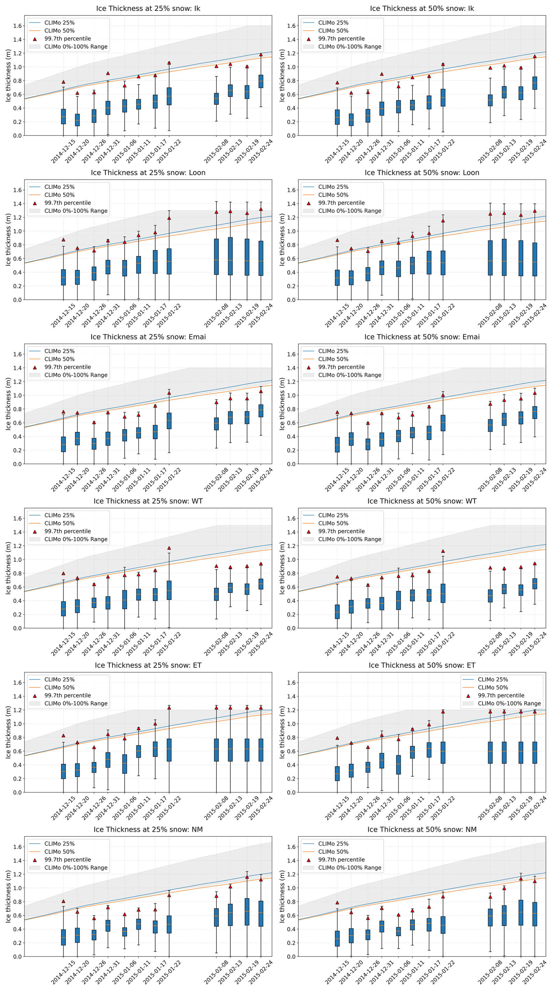
Figure 7Boxplots for InSAR-derived thickness, CLIMo simulation, and in situ measurements in Ikroavik Lake, Loon Lake, Emaiksoun Lake, West Twin Lake, and East Twin Lake. The red triangles indicate the 99.7th percentile of the InSAR-derived ice thickness distribution, which was used as the representative ice thickness for comparison with CLIMo simulations.
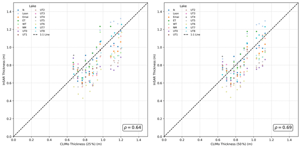
Figure 7 shows boxplots with the distribution of InSAR-derived LIT for each acquisition date for the five largest lakes in the study area and CLIMo simulations, with in-situ ice thickness measurements of West Twin Lake and Lake Emaiksoun. Due to space constraints, boxplots for the remaining lakes are provided in Fig. A1. Due to the small difference between CLIMo simulated LIT and in situ measurements for West Twin Lake and Emaiksoun Lake, the 25 % or 50 % snow cover scenarios show the best agreement for comparison and accuracy assessment with our InSAR-derived thickness. Figure 8 compares InSAR-derived LIT with CLIMo simulations under 25 % and 50 % snow scenarios. The majority of points cluster around the 1:1 line, indicating reasonable agreement in lake ice growth, with Spearman correlation of 0.64 and 0.69 compared to the CLIMo 25 % and 50 % scenarios, respectively. Across all dates, the median and interquartile ranges consistently fall below the simulated CLIMo thickness. Notably, the upper tail of the LIT distribution, as indicated by the 99.7th percentile, closely follows the seasonal growth pattern simulated by CLIMo.
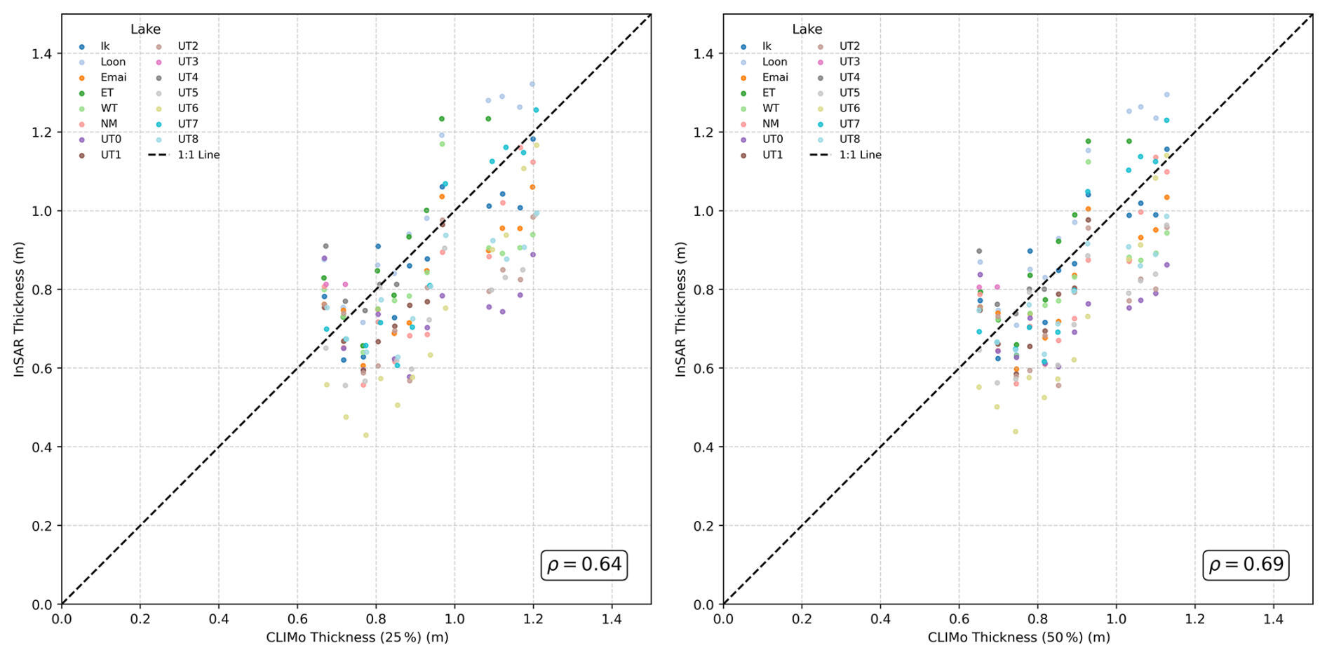
Figure 8Scatterplots comparing InSAR-derived lake ice thickness (LIT), represented by the 99.7th percentile of the InSAR-derived thickness distribution, with CLIMo-simulated LIT for each lake under the 25 % snow (left) and 50 % snow (right) scenarios. The Spearman correlation coefficients (ρ) are shown in each panel. Lakes that are fully frozen to the lake bed are omitted.
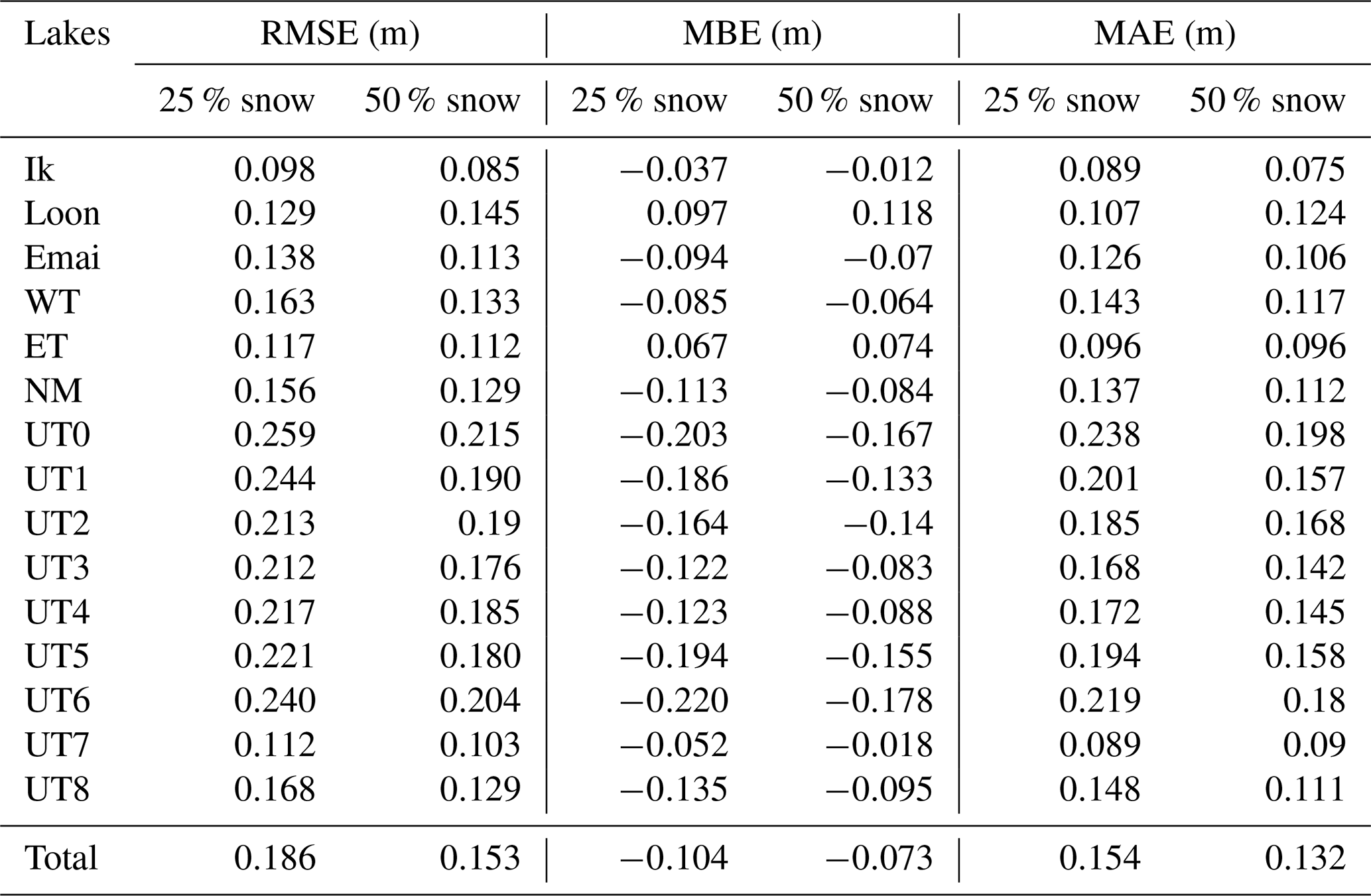
Table 5 summarizes the accuracy assessment of InSAR-derived LIT relative to CLIMo simulations for the study lakes under 25 % and 50 % snow cover. Overall, the results show moderate agreement between InSAR estimates and simulated thicknesses, with RMSE values typically ranging from approximately 0.09 to 0.26 cm. MAE values are similar in magnitude, typically between 0.08 and 0.24 m. Overall, the average RMSE for 25 % and 50 % snow cover scenarios is 0.186 and 0.153 m respectively, with an MBE of −0.104 and −0.073 m. For most lakes, the mean bias error (MBE) is predominantly negative, indicating that InSAR systematically underestimates LIT compared to CLIMo simulations.
Table 5Accuracy Assessment by comparing CLIMo simulations and InSAR-derived LIT at 99.7th percentile for each lake across all image acquisitions.
4.1 Coherence variability across ice types
One key advantage of using TanDEM-X pursuit monostatic mode for monitoring LIT is its ability to maintain high interferometric coherence due to the extremely short revisit period (9–10 s), effectively eliminating temporal decoherence effects caused by surface changes that would occur between traditional SAR revisit periods of 4–12 d (Chen and Gunn, 2025; Ferguson and Gunn, 2023; Siles et al., 2022). TanDEM-X data acquired in the pursuit monostatic mode consistently maintain high coherence values on dynamic surfaces such as glacial flows and lake ice growth, which mitigate the effect of temporal decorrelation (Hong et al., 2018; van der Sanden et al., 2018). Therefore, the pursuit of the monostatic TanDEM-X technique offers methodological advantages: its sustained coherence ensures stable phase unwrapping and reliable elevation conversion throughout dynamic lake-ice processes, whereas repeat-pass InSAR methods may fail under such variable ice-surface conditions.
Previous studies using repeat-pass InSAR for LIT retrieval have shown that coherence deteriorates sharply when lake ice deformation occurs between satellite passes – particularly when cracks and ice ridges form during the time interval (Ferguson and Gunn, 2023; Siles et al., 2022). Even minor ice surface displacements or deformations driven by internal stresses disrupt the phase relationship between the two observation sets, resulting in very low coherence that limits ice thickness retrieval. On the other hand, the TanDEM-X satellite has been shown to maintain high coherence even over active deformation features such as fractures and pressure ridges. Immediate interferometry methods ensure that the scattering geometry at the ice-water interface and within ice fractures remains largely unchanged, enabling stable phase inversion even in the presence of newly formed fractures. However, despite maintaining coherence, the radar-scattering mechanism in ice cracks fundamentally differs from that in floating or grounded ice. Ice deformation may expose water or complex geometries, meaning the observed phase center does not necessarily correspond to the ice-water interface (Gunn et al., 2017; Murfitt and Duguay, 2021). Consequently, high coherence does not guarantee that TanDEM-X thickness estimates at pressure ridges or relic leads reflect the true ice-bottom geometry, and LIT inversion results for these areas remain uncertain. Nevertheless, the persistent high coherence indicates that TanDEM-X can still capture stable phase information related to the structural properties of the ice fracture surface. While unusable for ice thickness retrieval, the phase signal in fractured regions may offer potential for future studies through immediate interferometry, which focuses on locating deformation characteristics, fracture mechanics, or other structural properties of lake ice pertinent for ice road construction or safe travel routing.
4.2 Floating vs. grounded ice
The interface between lake ice and the lake bed imposes constraints on obtaining LIT using interferometry, as the radar backscatter response is inherently weak in regions of grounded ice, reducing the reliability of phase measurements. When lake ice freezes directly onto the lake bed, lake sediments absorb the majority of SAR signals, producing only weak scattering in the X-band (Antonova et al., 2016). Consequently, SAR pixels observing bedfast ice are often dominated by noise rather than coherent echoes from a clearly defined ice-bed interface. Hence, interferometry can't directly monitor the thickness of grounded ice. During this study, grounded ice pixels are masked by testing the backscatter distribution for each lake, and the thickness values of grounded ice pixels are inverted to calculate the growth of floating ice pixels. Other approaches, such as inserting lake depth data for regions of grounded ice, are effective in shallow lake areas, but the accuracy of lake bathymetric products is a critical factor (Duguay and Lafleur, 2003). Also, it is crucial to consistently monitor lake depth to improve the LIT inversion, as lake depth and water level can change over time (Jones et al., 2023). Future research may attempt to utilize high-resolution lake bathymetric data, such as the lake bathymetric dataset generated by the Ice, Cloud, and land Elevation Satellite-2 (ICESat-2) Lidar Altimetry (Huang et al., 2025). The accuracy of grounded ice extraction can also be further validated using in-situ measurements, accounting for potential misclassification under wet-snow conditions.
4.3 Factors that affect TanDEM-X-derived accuracy
4.3.1 Height of Ambiguity
A key source of uncertainty in the TanDEM-X–derived lake ice thickness estimates arises from variations in the perpendicular baseline during image acquisitions. TanDEM-X perpendicular baselines vary because the satellites continuously adjust their relative orbits depending on mission objectives and operational constraints. The sensitivity of interferometric phase to surface height is directly proportional to the perpendicular baseline; when the baseline is small, the interferometric HoA increases, reducing the system's ability to resolve subtle vertical elevation differences (Krieger et al., 2005). As a result, DEMs generated under low-baseline conditions exhibit reduced vertical precision and are more susceptible to phase noises, residual flat-earth phase, and residual atmospheric effects. Consequently, the LIT retrieved from DEMs using a low perpendicular baseline (<50 m) may introduce errors in LIT estimation. During this study, we used TanDEM-X image acquisitions with perpendicular baselines greater than 100 m to avoid such impacts (Table 2). This resulted in HoA around 10–20 m in this study, which is capable of monitoring LIT (Hong et al., 2018). However, further investigation and analysis are crucial to confirm the impact of using different vertical baselines on lake ice thickness measurements across varying regional topography.
4.3.2 Shoreline topography and water level
It is important to note that accurate LIT retrieval using the immediate interferometric method in this study is sensitive to topographic effects; the precision of shoreline height estimation needs to reach the centimeter level to maintain high accuracy. This study manually digitized the lake extent to minimize such errors. However, developing automated algorithms for extracting lake boundaries is crucial for the accuracy of shoreline elevation extraction (van der Sanden et al., 2018; Chen and Gunn, 2025). Also, this study used the LiDAR-derived DSM acquired in 2018 to estimate the height difference between water level and surrounding topography, whereas the InSAR observations used to retrieve lake ice thickness were collected during the 2014–2015 winter season. Potential interannual changes in lake water levels between these periods may introduce uncertainty into the height-difference calculations, which directly affect the inferred ice thickness. Future studies would benefit from methods capable of accurately constraining lake water levels contemporaneously using altimetry, in-situ measurements, or the Surface Water and Ocean Topography (SWOT) mission designed to determine the hydrostatic level (Fu et al., 2024).
4.3.3 Scattering sources above the ice cover
The main limitation of the current LIT retrieval method is that using the 99.7th percentile for each lake does not guarantee the phase centre targeted at the ice-water interface. As an example, in West Twin Lake, although the mean thickness on 26 December 2014 is greater than 20 December 2014, the thickness value at the 99.7th percentile is lower (0.71 and 0.64 m, respectively). This indicates that in the former acquisition, some pixels are unaffected by scattering sources within the ice layer and reach the ice-water interface, whereas in the latter image, it is likely that the phase center was observed above the ice-water interface due to scattering events. Additionally, West Twin Lake showed greater underestimation in late winter than in the early winter. This might be due to thicker ice layers, which result in more scattering events affecting the phase center. As a result, using the 99.7th percentile approach still leads to underestimating LIT at some lakes and image acquisitions due to scattering events within the ice volume.
On the other hand, using the 99.7th percentile leads to an overestimation of LIT in some lakes, mostly distributed at the time of image acquisition on 15 December 2014 and 22 January 2015. This might be due to the two images having a smaller perpendicular baseline, which increases the interferometric noise, and increases the HoA (23 m compared to other acquisitions around 15 m).
4.3.4 Correction for dielectric properties in bubbled ice
An important consideration for InSAR-derived LIT is the dielectric permittivity assumed for wavelength compression within the ice column. While previous studies use a dielectric constant representative of clear, bubble-free freshwater ice (), natural lake ice often contains abundant air inclusions and internal heterogeneities that reduce the effective dielectric permittivity (Wegmüller et al., 2010). Bubble-rich ice, therefore, exhibits a lower effective ϵ′ compared to clear ice, which directly influences phase-to-thickness inversion. This study adopted a reduced dielectric constant of 2.97 to account for bubble inclusions, based on empirical estimates from the density of bubbled ice (Fujita et al., 2000; Zhang et al., 2023). This adjustment modifies the wavelength compression factor, resulting in estimated differences in lake ice thickness of approximately 1–3 cm. Although this magnitude may appear small relative to seasonal ice growth, it becomes considerable when monitoring LIT at high precision, such as the Global Climate Observing System (GCOS) ultimate goal of LIT uncertainty below 10 cm (World Meteorological Organization, 2022).
4.3.5 Other factors
In addition to phase-center error, although the freeboard height of floating ice with variable snow loading has been taken into account, this method did not account for the freeboard height from the snow ice formation. In the CLIMo simulation, the growth rate of the upper ice surface is extremely low, resulting in a total snow ice thickness under 1 cm. However, future research may consider incorporating snow ice formation to retrieve LIT. On the other hand, overestimation or underestimation of LIT from CLIMo might exist, since the weather station data used in this study originate from Utqiaġvik Airport; the actual atmospheric conditions over the lakes may vary slightly. Lake depth provided from the hydroLAKES dataset might be incorrect; for lake UT3 and UT4, both lakes were fully frozen to bed in the early winter season, but the dataset estimated lake depth around 2 m, which is inconsistent with observed ice phenology, leading to our CLIMo simulation not being bounded by the actual lake depth. Additionally, CLIMo simulations might overestimate LIT in shallow thermokarst lakes due to under-ice heating from taliks or lake sediments, as CLIMo adopted a fixed heat flux from the lake bottom (Rafat et al., 2023). Future analysis should integrate in-situ observations and explore the capability of TanDEM-X interferometry to monitor LIT under varying ice conditions and acquisition configurations.
4.4 Comparison with current radar altimetry studies
Although the TanDEM-X bistatic InSAR approach investigated here currently exhibits lower quantitative accuracy than recent radar altimetry-based LIT retrievals, it provides a fundamentally different and potentially complementary measurement strategy. In the present study, the mean RMSE is approximately 0.16–0.18 m, whereas recent radar altimetry studies have demonstrated accuracies ranging from approximately 0.03–0.10 m (Mangilli et al., 2022, 2024). Radar altimetry retrieves LIT primarily from the separation of waveform features associated with the snow–ice and ice–water interfaces, with recent retracking algorithms substantially improving the precision of this approach (Mangilli et al., 2022, 2024). In contrast, the TanDEM-X approach estimates the elevation of the dominant interferometric phase center, which is influenced by microwave penetration and scattering within the ice–snow system. Hence, the current TanDEM-X immediate interferometry approach is limited due to attenuation or scattering events at the bubbled ice layer. However, an important potential advantage of the InSAR approach is not only its two-dimensional spatial coverage, but using the InSAR approach at longer wavelengths in future might also have the potential to retrieve more accurate LIT compared to radar altimetry. Where the uncertainty due to the sensitivity of radar altimetry to snow and volume-scattering effects remains an important consideration, the impact of snow might shift the location of the first echo toward the snow surface from the snow-ice interface and lead to overestimation of LIT that is observed in Mangilli et al. (2024). Similarly, volume scattering within bubble-rich freshwater ice may alter the waveform response and complicate identification of the ice–water interface, where its effect hasn't been investigated by current Ku-band radar altimetry studies (Li et al., 2023; Mangilli et al., 2022, 2024). These effects motivate further investigation of longer-wavelength bistatic InSAR, which reduces sensitivity to volume scattering from snow and ice bubble inclusions, and potentially provides a more stable estimate of the dominant ice–water scattering phase center.
This study utilizes TanDEM-X pursuit-mode interferometry to retrieve lake ice thickness in Alaskan thermokarst lakes; the immediate interferometric method minimized temporal decorrelation, thereby reducing errors due to low coherence. By conducting an accuracy assessment of InSAR-derived thickness using CLIMo simulations and in-situ measurements, the method proposed in this study provides a framework for interferometry-derived lake ice thickness retrievals. This study maintains sufficient coherence in lake ice thickness retrieval using immediate interferometric technology and reveals that scatterers within the ice cover are another important factor affecting ice thickness retrieval. This provides a deeper understanding and additional insights for future ice thickness retrieval technology, indicating that using SAR instruments such as NISAR and TanDEM-L with longer wavelengths while maintaining high coherence has significant potential for accurate, high-resolution retrieval of lake ice thickness (Huber et al., 2018; Kellogg et al., 2020).
Future advances in LIT retrieval using InSAR while ensuring high coherence should focus on better quantifying radar scattering processes within the ice column. A major source of uncertainty in InSAR-derived LIT is the displacement of the effective phase center from the ice–water interface due to volume scattering from bubble inclusions. Physically based forward modelling, such as the Snow Microwave Radiative Transfer (SMRT) framework, provides a promising approach for simulating radar interactions with layered snow and ice media and for assessing how variations in ice properties influence penetration depth and phase contributions (Picard et al., 2018; Murfitt et al., 2023). In addition, polarimetric techniques, including scattering decomposition and polarimetric interferometry (Pol-InSAR), offer the potential to separate scattering mechanisms and estimate the vertical distribution of scattering within the ice column, thereby enabling more accurate characterization of the phase center location (Cloude and Pottier, 2002). To support methodological improvements, future studies would benefit from expanded in situ measurements that document lake ice internal structure, such as bubble content and density profiles in different ice layers. Such observations are critical for parameterizing electromagnetic models, validating phase-center interpretations, and improving the physical basis of InSAR-derived lake ice thickness estimates. Beyond that, future satellite missions operating at longer wavelengths are expected to mitigate phase-center bias by reducing sensitivity to small-scale heterogeneities as they propagate through the ice cover. In particular, recently released L-band missions, such as NISAR, proposed TanDEM-L, and the ESA Harmony mission, are expected to improve the retrieval of lake ice thickness by enhancing sensitivity to the ice–water interface (Huber et al., 2018; Kellogg et al., 2020).
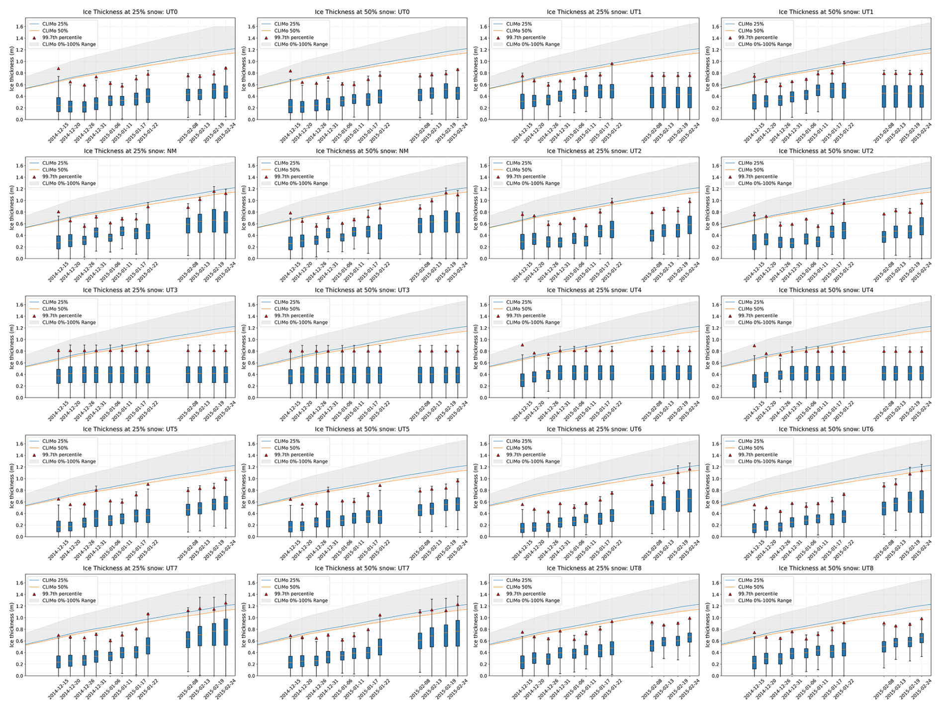
Figure A1Boxplots for InSAR-derived thickness and CLIMo simulation in other lakes. The red triangles indicate the 99.7th percentile of the InSAR-derived ice thickness distribution, which was used as the representative ice thickness for comparison with CLIMo simulations.
TanDEM-X data sharing is governed by licensing agreements from the German Aerospace Center (DLR). Value-added data products derived from TanDEM-X acquisitions are available upon request by the author(s) under a data sharing agreement. The code can be obtained upon request from the corresponding author.
Conceptualization, PC and GG; methodology, PC and GG; validation, PC and GG; formal analysis, PC; investigation, PC; data curation, PC and GG; writing – original draft preparation, PC and GG; writing – review and editing, PC and GG; visualization, PC, GG, and SK; supervision, GG; project administration, GG; All authors have read and agreed to the published version of the manuscript.
The contact author has declared that none of the authors has any competing interests.
Publisher's note: Copernicus Publications remains neutral with regard to jurisdictional claims made in the text, published maps, institutional affiliations, or any other geographical representation in this paper. The authors bear the ultimate responsibility for providing appropriate place names. Views expressed in the text are those of the authors and do not necessarily reflect the views of the publisher.
TanDEM-X data was accessed through the Coregistered Single look Slant range Complex (COSSC) data proposal ATI_HYDR7416 through the Science Service System (https://tandemx-science.dlr.de/, last access: 7 April 2026), and original acquisitions are copyright of DLR. Thanks to Christopher Arp and Ken Hinkel providing in-situ measurements for this study.
This research was funded by the National Science and Engineering Research Council of Canada Discovery Grant to Grant Gunn (grant no. RGPIN-2021-02742).
This paper was edited by Homa Kheyrollah Pour and reviewed by two anonymous referees.
Alaska Climate Research Center: Climate normal, https://akclimate.org/data/, last access: 8 January 2026.
Amani, M., Poncos, V., Brisco, B., Foroughnia, F., DeLancey, E. R., and Ranjbar, S.: InSAR coherence analysis for wetlands in Alberta, Canada using time-series Sentinel-1 data, Remote Sens., 13, 3315, https://doi.org/10.3390/rs13163315, 2021.
Antonova, S., Duguay, C. R., Kääb, A., Heim, B., Langer, M., Westermann, S., and Boike, J.: Monitoring bedfast ice and ice phenology in lakes of the Lena River delta using TerraSAR-X backscatter and coherence time series, Remote Sens., 8, 903, https://doi.org/10.3390/rs8110903, 2016.
Arp, C. D., Jones, B. M., Engram, M., Alexeev, V. A., Cai, L., Parsekian, A., Hinkel, K., Bondurant, A. C., and Creighton, A.: Contrasting lake ice responses to winter climate indicate future variability and trends on the Alaskan Arctic Coastal Plain, Environ. Res. Lett., 13, 125001, https://doi.org/10.1088/1748-9326/aae994, 2018.
Bamler, R. and Hartl, P.: Synthetic aperture radar interferometry, Inverse Probl., 14, R1–R54, https://doi.org/10.1088/0266-5611/14/4/001, 1998.
Beckers, J. F., Alec Casey, J., and Haas, C.: Retrievals of Lake Ice Thickness From Great Slave Lake and Great Bear Lake Using CryoSat-2, IEEE T. Geosci. Remote, 55, 3708–3720, https://doi.org/10.1109/TGRS.2017.2677583, 2017.
Box, J. E., Colgan, W. T., Christensen, T. R., Schmidt, N. M., Lund, M., Parmentier, F. J. W., Brown, R., Bhatt, U. S., Euskirchen, E. S., Romanovsky, V. E., and Walsh, J. E.: Key indicators of Arctic climate change: 1971–2017, Environ. Res. Lett., 14, 045010, https://doi.org/10.1088/1748-9326/aafc1b, 2019.
Brown, L. C. and Duguay, C. R.: The response and role of ice cover in lake–climate interactions, Prog. Phys. Geogr., 34, 671–704, https://doi.org/10.1177/0309133310375653, 2010.
Brown, L. C. and Duguay, C. R.: A comparison of simulated and measured lake ice thickness using a Shallow Water Ice Profiler, Hydrol. Process., 25, 2932–2941, https://doi.org/10.1002/hyp.8087, 2011.
Carson, C. E. and Hussey, K. M.: The oriented lakes of Arctic Alaska, J. Geol., 70, 417–439, https://doi.org/10.1086/626857, 1962.
Chen, C. W. and Zebker, H. A.: Phase unwrapping for large SAR interferograms: Statistical segmentation and generalized network models, IEEE T. Geosci. Remote, 40, 1709–1719, https://doi.org/10.1109/TGRS.2002.802453, 2002.
Chen, P. and Gunn, G.: Surface water extent extraction in prairie environments using Sentinel-1 image-pair coherence, Glacies, 2, 6, https://doi.org/10.3390/glacies2020006, 2025.
Cloude, S. R. and Pottier, E.: An entropy based classification scheme for land applications of polarimetric SAR, IEEE T. Geosci. Remote, 35, 68–78, https://doi.org/10.1109/36.551935, 2002.
Dewitz, J.: National Land Cover Database (NLCD) 2016 – Alaska, U.S. Geological Survey [data set], https://doi.org/10.5066/P96HHBIE, 2020.
Domine, F., Gallet, J., Bock, J., and Morin, S.: Structure, specific surface area and thermal conductivity of the snowpack around Barrow, Alaska, J. Geophys. Res., 117, 2011JD016647, https://doi.org/10.1029/2011JD016647, 2012.
Duguay, C. R. and Lafleur, P. M.: Determining depth and ice thickness of shallow sub-Arctic lakes using space-borne optical and SAR data, Int. J. Remote Sens., 24, 475–489, https://doi.org/10.1080/01431160304992, 2003.
Duguay, C. R., Pultz, T. J., Lafleur, P. M., and Drai, D.: RADARSAT backscatter characteristics of ice growing on shallow sub-Arctic lakes, Churchill, Manitoba, Canada, Hydrol. Process., 16, 1631–1644, https://doi.org/10.1002/hyp.1010, 2002.
Duguay, C. R., Flato, G. M., Jeffries, M. O., Ménard, P., Morris, K., and Rouse, W. R.: Ice‐cover variability on shallow lakes at high latitudes: model simulations and observations, Hydrol. Process., 17, 3465–3483, https://doi.org/10.1002/hyp.1394, 2003.
Duguay, C. R., Bernier, M., Gauthier, Y., and Kouraev, A.: Remote sensing of lake and river ice, in: Remote Sensing of the Cryosphere, edited by: Tedesco, M., John Wiley & Sons, Ltd., 273–306, https://doi.org/10.1002/9781118368909.ch12, 2015.
Engram, M., Anthony, K. W., Meyer, F. J., and Grosse, G.: Synthetic aperture radar (SAR) backscatter response from methane ebullition bubbles trapped by thermokarst lake ice, Can. J. Remote Sens., 38, 667–682, https://doi.org/10.5589/m12-054, 2013a.
Engram, M., Anthony, K. W., Meyer, F. J., and Grosse, G.: Characterization of L-band synthetic aperture radar (SAR) backscatter from floating and grounded thermokarst lake ice in Arctic Alaska, The Cryosphere, 7, 1741–1752, https://doi.org/10.5194/tc-7-1741-2013, 2013b.
Engram, M., Arp, C. D., Jones, B. M., Ajadi, O. A., and Meyer, F. J.: Analyzing floating and bedfast lake ice regimes across Arctic Alaska using 25 years of space-borne SAR imagery, Remote Sens. Environ., 209, 660–676, https://doi.org/10.1016/j.rse.2018.02.022, 2018.
Ferguson, J. and Gunn, G. E.: Monitoring Lake Ice Thickness Growth Using SAR Interferometry, in: AGU Fall Meeting Abstracts, San Francisco, CA, USA, 11–15 December 2023, C33F-1465, 2023.
Fletcher, K., European Space Agency, and European Space Research and Technology Centre (Eds.): InSAR principles: guidelines for SAR interferometry processing and interpretation, ESA Publications, ESTEC, Noordwijk, the Netherlands, 1 p., 2007.
Fu, L. L., Pavelsky, T., Cretaux, J. F., Morrow, R., Farrar, J. T., Vaze, P., and Dibarboure, G.: The surface water and ocean topography mission: A breakthrough in radar remote sensing of the ocean and land surface water, Geophys. Res. Lett., 51, e2023GL107652, https://doi.org/10.1029/2023GL107652, 2024.
Fujita, S., Matsuoka, T., Ishida, T., Matsuoka, K., and Mae, S.: A summary of the complex dielectric permittivity of ice in the megahertz range and its applications for radar sounding of polar ice sheets, in: Physics of ice core records, Hokkaido University Press, 185–212, 2000.
Goldstein, R. M. and Werner, C. L.: Radar interferogram filtering for geophysical applications, Geophys. Res. Lett., 25, 4035–4038, https://doi.org/10.1029/1998GL900033, 1998.
Gunn, G. E., Duguay, C. R., Brown, L. C., King, J., Atwood, D., and Kasurak, A.: Freshwater lake ice thickness derived using surface-based X- and Ku-band FMCW scatterometers, Cold Reg. Sci. Technol., 120, 115–126, https://doi.org/10.1016/j.coldregions.2015.09.001, 2015.
Gunn, G. E., Duguay, C. R., Derksen, C., Clausi, D. A., and Toose, P.: Investigating the influence of variable freshwater ice types on passive and active microwave observations, Remote Sens., 9, 1242, https://doi.org/10.3390/rs9121242, 2017.
Gunn, G. E., Duguay, C. R., Atwood, D. K., King, J., and Toose, P.: Observing scattering mechanisms of bubbled freshwater lake ice using polarimetric RADARSAT-2 (C-band) and UW-Scat (X- and Ku-bands), IEEE T. Geosci. Remote, 56, 2887–2903, https://doi.org/10.1109/TGRS.2017.2786158, 2018.
Hampton, S. E., Galloway, A. W. E., Powers, S. M., Ozersky, T., Woo, K. H., Batt, R. D., Labou, S. G., O'Reilly, C. M., Sharma, S., Lottig, N. R., Stanley, E. H., North, R. L., Stockwell, J. D., Adrian, R., Weyhenmeyer, G. A., Arvola, L., Baulch, H. M., Bertani, I., Bowman, L. L., and Xenopoulos, M. A.: Ecology under lake ice, Ecol. Lett., 20, 98–111, https://doi.org/10.1111/ele.12699, 2017.
Hallikainen, M.: Dielectric properties of sea ice at microwave frequencies, NASA STI/Recon Tech. Rep. N, 78, 11293, 1977.
Heidinger, A. K., Foster, M. J., Walther, A., Zhao, X., and NOAA CDR Program: NOAA Climate Data Record (CDR) of Cloud Properties from AVHRR Pathfinder Atmospheres – Extended (PATMOS-x), Version 5.3 (Version Superseded), NOAA [data set], https://doi.org/10.7289/V5348HCK, 2014.
Hirose, T., Kapfer, M., Bennett, J., Cott, P., Manson, G., and Solomon, S.: Bottomfast ice mapping and the measurement of ice thickness on tundra lakes using C-band synthetic aperture radar remote sensing, J. Am. Water Resour. Assoc., 44, 285–292, https://doi.org/10.1111/j.1752-1688.2007.00146.x, 2008.
Hong, S. H., Wdowinski, S., Amelung, F., Kim, H. C., Won, J. S., and Kim, S. W.: Using TanDEM-X pursuit monostatic observations with a large perpendicular baseline to extract glacial topography, Remote Sens., 10, 1851, https://doi.org/10.3390/rs10111851, 2018.
Huang, C. H., Zhang, S., Shah, D., Yadav, A., Li, Y., Zhao, G., and Gao, H.: 3D-LAKES: Three-Dimensional Global Lake and Reservoir Bathymetry from ICESat-2 Altimetry and Landsat Imagery, Sci. Data, 12, 1625, https://doi.org/10.1038/s41597-025-05911-y, 2025.
Huber, S., De Almeida, F. Q., Villano, M., Younis, M., Krieger, G., and Moreira, A.: Tandem-L: A Technical Perspective on Future Spaceborne SAR Sensors for Earth Observation, IEEE T. Geosci. Remote, 56, 4792–4807, https://doi.org/10.1109/TGRS.2018.2837673, 2018.
Jeffries, M. O., Morris, K., Weeks, W. F., and Wakabayashi, H.: Structural and stratigraphic features and ERS-1 synthetic aperture radar backscatter characteristics of ice growing on shallow lakes in NW Alaska, winter 1991–1992, J. Geophys. Res.-Oceans, 99, 22459–22471, https://doi.org/10.1029/94JC01479, 1994.
Jones, B. M., Kanevskiy, M. Z., Parsekian, A. D., Bergstedt, H., Ward Jones, M. K., Rangel, R. C., and Shur, Y.: Rapid saline permafrost thaw below a shallow thermokarst lake in Arctic Alaska, Geophys. Res. Lett., 50, e2023GL105552, https://doi.org/10.1029/2023GL105552, 2023.
Kellogg, K., Hoffman, P., Standley, S., Shaffer, S., Rosen, P., Edelstein, W., and Sarma, C. V. H. S.: NASA-ISRO synthetic aperture radar (NISAR) mission, in: 2020 IEEE Aerospace Conference, March 2020, 1–21, https://doi.org/10.1109/AERO47225.2020.9172542, 2020.
Krieger, G., Fiedler, H., Hajnsek, I., Eineder, M., Werner, M., and Moreira, A.: TanDEM-X: mission concept and performance analysis, in: IEEE International Geoscience and Remote Sensing Symposium (IGARSS), 4890–4893, 2005.
Leconte, R., Daly, S., Gauthier, Y., Yankielun, N., Bérubé, F., and Bernier, M.: A controlled experiment to retrieve freshwater ice characteristics from an FM-CW radar system, Cold Reg. Sci. Technol., 55, 212–220, https://doi.org/10.1016/j.coldregions.2008.07.005, 2009.
Li, X., Long, D., Huang, Q., and Zhao, F.: The state and fate of lake ice thickness in the Northern Hemisphere, Sci. Bull., 67, 537–546, https://doi.org/10.1016/j.scib.2021.12.015, 2022.
Li, X., Long, D., Cui, Y., Liu, T., Lu, J., Hamouda, M. A., and Mohamed, M. M.: Ice thickness and water level estimation for ice-covered lakes with satellite altimetry waveforms and backscattering coefficients, The Cryosphere, 17, 349–369, https://doi.org/10.5194/tc-17-349-2023, 2023.
Mangilli, A., Thibaut, P., Duguay, C. R., and Murfitt, J.: A New Approach for the Estimation of Lake Ice Thickness From Conventional Radar Altimetry, IEEE T. Geosci. Remote, 60, 1–15, https://doi.org/10.1109/TGRS.2022.3186253, 2022.
Mangilli, A., Duguay, C. R., Murfitt, J., Moreau, T., Amraoui, S., Mugunthan, J. S., Thibaut, P., and Donlon, C.: Improving the estimation of lake ice thickness with high-resolution radar altimetry data, Remote Sens., 16, 2510, https://doi.org/10.3390/rs16142510, 2024.
McRae-Pharo, C.: Polarimetric decomposition of fully polarimetric synthetic aperture RADAR to examine freshwater lake ice microwave backscatter behaviour, M.Sc. thesis, University of Waterloo, https://hdl.handle.net/10012/21669 (last access: 7 April 2026), 2025.
Ménard, P., Duguay, C. R., Flato, G. M., and Rouse, W. R.: Simulation of ice phenology on Great Slave Lake, Northwest Territories, Canada, Hydrol. Process., 16, 3691–3706, https://doi.org/10.1002/hyp.1234, 2002.
Messager, M. L., Lehner, B., Grill, G., Nedeva, I., and Schmitt, O.: Estimating the volume and age of water stored in global lakes using a geo-statistical approach, Nat. Commun., 7, 13603, https://doi.org/10.1038/ncomms13603, 2016.
Morris, K., Jeffries, M., and Duguay, C.: Model simulation of the effects of climate variability and change on lake ice in central Alaska, USA, Ann. Glaciol., 40, 113–118, https://doi.org/10.3189/172756405781813663, 2005.
Murfitt, J. and Duguay, C. R.: 50 years of lake ice research from active microwave remote sensing: Progress and prospects, Remote Sens. Environ., 264, 112616, https://doi.org/10.1016/j.rse.2021.112616, 2021.
Murfitt, J. C., Brown, L. C., and Howell, S. E.: Estimating lake ice thickness in central Ontario, PLOS ONE, 13, e0208519, https://doi.org/10.1371/journal.pone.0208519, 2018.
Murfitt, J., Duguay, C., Picard, G., and Gunn, G.: Forward modelling of synthetic aperture radar backscatter from lake ice over Canadian Subarctic lakes, Remote Sens. Environ., 286, 113424, https://doi.org/10.1016/j.rse.2022.113424, 2023.
Murfitt, J., Duguay, C., Picard, G., and Lemmetyinen, J.: Forward modelling of synthetic-aperture radar (SAR) backscatter during lake ice melt conditions using the Snow Microwave Radiative Transfer (SMRT) model, The Cryosphere, 18, 869–888, https://doi.org/10.5194/tc-18-869-2024, 2024.
Olefeldt, D., Goswami, S., Grosse, G., Hayes, D., Hugelius, G., Kuhry, P., McGuire, A. D., Romanovsky, V. E., Sannel, A. B. K., Schuur, E. A. G., and Turetsky, M. R.: Circumpolar distribution and carbon storage of thermokarst landscapes, Nat. Commun., 7, 13043, https://doi.org/10.1038/ncomms13043, 2016.
Ozersky, T., Poste, A., Rautio, M., and Leu, E.: Impacts of changing winters on lake ecosystems will increase with latitude, Ecol. Lett., 28, e70200, https://doi.org/10.1111/ele.70200, 2025.
Perrin, A., Dion, J., Eng, S., Sawyer, D., Nodelman, J. R., Comer, N., Auld, H., Sparling, E., Harris, M., Nodelman, J. Y. H., and Kinnear, L.: Economic implications of climate change adaptations for mine access roads in Northern Canada, Northern Climate ExChange, Yukon Research Centre, Yukon College, 2015.
Picard, G., Sandells, M., and Löwe, H.: SMRT: an active–passive microwave radiative transfer model for snow with multiple microstructure and scattering formulations (v1.0), Geosci. Model Dev., 11, 2763–2788, https://doi.org/10.5194/gmd-11-2763-2018, 2018.
Pietroniro, A. and Leconte, R.: A review of Canadian remote sensing and hydrology, 1999–2003, Hydrol. Process., 19, 285–301, https://doi.org/10.1002/hyp.5760, 2005.
Rafat, A., Pour, H. K., Spence, C., Palmer, M. J., and MacLean, A.: An analysis of ice growth and temperature dynamics in two Canadian subarctic lakes, Cold Reg. Sci. Technol., 210, 103808, https://doi.org/10.1016/j.coldregions.2023.103808, 2023.
Rafat, A., Cheng, B., and Pour, H. K.: Exploring the physics of two thermodynamic lake ice models, Water Resour. Res., 61, e2024WR038615, https://doi.org/10.1029/2024WR038615, 2025.
Rizzoli, P., Martone, M., Gonzalez, C., Wecklich, C., Tridon, D. B., Bräutigam, B., Schulze, D., Zink, M., Bachmann, M., Krieger, G., and Moreira, A.: Generation and performance assessment of the global TanDEM-X digital elevation model, ISPRS J. Photogramm. Remote, 132, 119–139, https://doi.org/10.1016/j.isprsjprs.2017.08.008, 2017.
Siles, G., Leconte, R., and Peters, D. L.: Retrieval of Lake Ice Characteristics from SAR Imagery, Can. J. Remote Sens., 48, 379–399, https://doi.org/10.1080/07038992.2022.2042227, 2022.
Stebler, O., Meier, E., and Nüesch, D.: Multi-baseline polarimetric SAR interferometry – first experimental spaceborne and airborne results, ISPRS J. Photogramm. Remote, 56, 149–166, https://doi.org/10.1016/S0924-2716(01)00049-1, 2002.
Sturm, M. and Liston, G. E.: The snow cover on lakes of the Arctic Coastal Plain of Alaska, USA, J. Glaciol., 49, 370–380, https://doi.org/10.3189/172756503781830539, 2003.
Surdu, C. M., Duguay, C. R., Brown, L. C., and Fernández Prieto, D.: Response of ice cover on shallow lakes of the North Slope of Alaska to contemporary climate conditions (1950–2011): radar remote-sensing and numerical modeling data analysis, The Cryosphere, 8, 167–180, https://doi.org/10.5194/tc-8-167-2014, 2014.
Surdu, C. M., Duguay, C. R., Pour, H. K., and Brown, L. C.: Ice freeze-up and break-up detection of shallow lakes in Northern Alaska with spaceborne SAR, Remote Sens., 7, 6133–6159, https://doi.org/10.3390/rs70506133, 2015.
Touzi, R., Lopes, A., Bruniquel, J., and Vachon, P. W.: Coherence estimation for SAR imagery, IEEE T. Geosci. Remote, 37, 135–149, https://doi.org/10.1109/36.739146, 2002.
U.S. Geological Survey: 2018 USGS lidar: North Slope Borough communities, AK – QL1 and QL2, NOAA [data set], https://www.fisheries.noaa.gov/inport/item/63140 (last access: 7 April 2026), 2019.
van der Sanden, J. J., Short, N. H., and Drouin, H.: InSAR coherence for automated lake ice extent mapping: TanDEM-X bistatic and pursuit monostatic results, Int. J. Appl. Earth Obs., 73, 605–615, https://doi.org/10.1016/j.jag.2018.07.015, 2018.
Vincent, L. A., Wang, X. L., Milewska, E. J., Wan, H., Yang, F., and Swail, V.: A second generation of homogenized Canadian monthly surface air temperature for climate trend analysis, J. Geophys. Res.-Atmos., 117, D18110, https://doi.org/10.1029/2012JD017859, 2012.
Wakabayashi, H., Motohashi, K., and Maezawa, N.: Monitoring Lake Ice in Northern Alaska with Backscattering and Interferometric Approaches Using Sentinel-1 Sar Data, in: IGARSS 2019 – 2019 IEEE International Geoscience and Remote Sensing Symposium, 4202–4205, https://doi.org/10.1109/IGARSS.2019.8900371, 2019.
Weeks, W. F., Gow, A. J., and Schertler, R. J.: Ground-truth observations of ice-covered North Slope lakes imaged by radar, CRREL Rep. 81-19, U.S. Army Cold Regions Research and Engineering Laboratory, Hanover, New Hampshire, USA, 1981
Wegmüller, U., Santoro, M., Werner, C., Strozzi, T., and Wiesmann, A.: Estimation of ice thickness of tundra lakes using ERS-ENVISAT cross-interferometry, in: 2010 IEEE International Geoscience and Remote Sensing Symposium, Honolulu, HI, USA, 25–30 July 2010, 316–319, https://doi.org/10.1109/IGARSS.2010.5649026, 2010.
Woodhouse, I. H.: Introduction to microwave remote sensing, Taylor&Francis, Boca Raton, 370 pp., 2006.
World Meteorological Organization: The 2022 GCOS ECVs Requirements (GCOS 245), 244 pp., https://library.wmo.int/idurl/4/58111 (last access: 11 November 2026), 2022.
Zhang, M., Chen, F., Guan, W., and Zhao, H.: Rapid thinning of lake ice for Himalayan glacial lakes since 2010, Remote Sens. Environ., 332, 115062, https://doi.org/10.1016/j.rse.2025.115062, 2026.
Zhang, Y., Fregona, M., Loehr, J., Ala-Könni, J., Song, S., Leppäranta, M., and Li, Z.: A field study on ice melting and breakup in a boreal lake, Pääjärvi, in Finland, The Cryosphere, 17, 2045–2058, https://doi.org/10.5194/tc-17-2045-2023, 2023.
Zink, M., Bachmann, M., Bräutigam, B., Fritz, T., Hajnsek, I., Moreira, A., and Krieger, G.: TanDEM-X: The new global DEM takes shape, IEEE Geosci. Remote Sens. Mag., 2, 8–23, https://doi.org/10.1109/MGRS.2014.2318895, 2014.