Improved subglacial boundary conditions near Dome C, Antarctica, through rigorous integration of multi-campaign radar data and an ensemble stochastic simulation approach

Subglacial bed topography is a fundamental boundary condition for ice-sheet flow, basal thermal regimes, and the preservation of palaeoclimate records, yet it remains highly uncertain across Antarctica. We use stochastic simulation methods to generate an ensemble of gridded (500 m) ice thickness and bed elevation near Dome C, and map bed elevation uncertainty accounting for impacts of data availability and basal roughness. New airborne radar measurements uncover previously undocumented sectors of the ice-bed interface and we integrate these with existing data using a rigorous approach to ensure nearby measurement compatibility. Our simulated bed shows improved representation of basal roughness between survey profiles, revealing regional roughness over 50 % higher than previous interpolations. We apply the ensemble to investigate uncertainty in meltwater routing, identifying well-constrained drainage away from the Dome C Plateau but poorly constrained outflow from Concordia Lake and parts of the Belgica Highlands. Topographic focussing of geothermal heat could lead to local anomalies up to ±30 % relative to the regional value, and several ice core drill sites are in a zone with potentially 12 % locally-reduced geothermal heating which could be favourable for deep ice layer preservation. This work demonstrates that the critical subglacial bed boundary condition is better represented by ensemble-based, stochastic simulations based on strictly cross-validated data rather than single deterministic interpolations, and simulated beds can improve the reliability of analyses with robust consideration of uncertainties in data-sparse regions.

1 Introduction

Kilometer-scale subglacial topography influences basal thermal state through locally variable pressure-melting (Cuffey and Paterson, 2010) and also modulates the effective area for geothermal heat conduction (van der Veen et al., 2007). While basal roughness can be constrained in high resolution in the along-track orientation of radar profiles, this information is missing between survey profiles. Widely-used interpolation methods such as kriging and splines do not preserve the spatial statistics of measurements in data gaps, leading to over-smoothing in gridded products and unrealistic patterns in basal roughness. Compared with single-grid, elevation-preserving products such as Bedmap3 (Pritchard et al., 2025) and Bedmachine v4 (Morlighem, 2026), texture-preserving bed gridding approaches can provide more realistic boundary conditions for model projections (McCormack et al., 2026). While requiring an ensemble-based framework which increases computational cost and methodological complexity, this approach generates spatially explicit uncertainty estimates to propagate into models and can be used to prioritise sites for future geophysical surveys. Sequential Gaussian Simulation (SGS) is one texture-preserving geostatistical method that simulates values between measurements based on the values and statistical properties of nearby data (Deutsch and Journel, 1997). This approach has been applied to generate ensembles of equally-likely bed elevation grids to investigate the basal environment, subglacial meltwater drainage, and geothermal heat flow (GHF) with robust consideration of the impacts of elevation uncertainty and realistic basal roughness (MacKie et al., 2020; MacKie et al., 2021; Shackleton et al., 2023).

Subglacial topography around Dome C is of particular interest in the context of paleoclimate investigations. Oxygen isotope records from marine sediment cores indicate that global glacial-interglacial cycles experienced a major shift in periodicity from 41 Ka to ca. 100 Ka between 1.4 Ma and 800 Ka BP (Lisiecki and Raymo, 2005). The underlying mechanisms for this Mid-Pleistocene Transition (MPT) are not yet fully constrained (Berends et al., 2021), but deep ice cores that preserve atmospheric gases from the palaeo-climate could provide continuous, high-resolution climate records. Ice layers that span the last 1.5 Ma could be located near the base of thick ice domes in the interior of Antarctica, though basal melting, ice flow, and accretion should be minimal to preserve ice layer stratigraphy (Fischer et al., 2013; Van Liefferinge and Pattyn, 2013). To locate basal ice with undisturbed stratigraphy and sufficient age resolution spanning the MPT, the ice core community is trying to delineate sites with: (1) ice around 2500 m thick, sufficient to resolve the MPT without inducing significant basal-melting; (2) low surface accumulation to limit vertical strain-induced thinning of ice layers; (3) low basal roughness to prevent disruption of basal ice stratigraphy through lateral strain; (4) low GHF to restrict basal melting and preserve the oldest ice layers. The European Project for Ice Coring in Antarctica (EPICA) successfully retrieved a 3260 m long ice core near Dome C, Antarctica that provides climate records for the last 800 Ka (Jouzel et al., 2007; Lüthi et al., 2008).

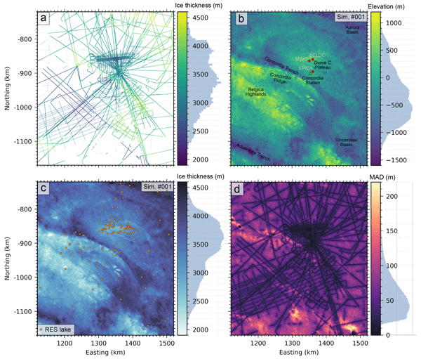
Ice thickness, basal roughness, and GHF are critical boundary conditions for thermomechanical modelling which delineate promising drill sites in the Dome C region that could resolve the MPT (Chung et al., 2023b; Parrenin et al., 2017; Passalacqua et al., 2017; Van Liefferinge et al., 2018; Wang et al., 2023; Young et al., 2017). Subglacial topography and ice thickness variability near Dome C (Fig. 1a–c) is documented in radar surveys (Drewry et al., 1982; Forieri et al., 2004; Tabacco et al., 1998), with thinner ice (<2.5 km) observed over the Belgica Highlands and Concordia Ridge, and 2.5–3.5 km thick ice over the Dome C Plateau. Ice thicknesses over 4 km are located above Concordia and Vincennes subglacial lakes and in the Concordia Trench, with up to 4.7 km reported in the Aurora Subglacial Basin. The Concordia Trench and Adventure Trench are tectonic features 20–50 km in width with over 1 km thicker ice than the surroundings, oriented approximately northeast – southwest (Cianfarra et al., 2009). Spatial coverage of surveys varies from the well-resolved topography over the Dome C Plateau and surrounding Concordia Station, to large data gaps over Vincennes Basin and southwest Belgica Highlands (Fig. 1).

Figure 1 Region map, radar survey data, and simulation results. (a) Radar-derived ice thickness measurements in the Dome C region. (b) Simulated bed elevation #001 from the ensemble of 100, with Concordia Station (green triangle) and ice cores plotted (red square). (c) Simulated ice thickness #001 from the ensemble of 100, with subglacial lakes (orange circle) inferred from compiled radio-echo sounding (RES) analyses (Livingstone et al., 2022). (d) Median Absolute Deviation (MAD) over the ensemble of 100 simulated bed elevation grids. All maps are projected to EPSG:3031. Histograms alongside colour bars show the distribution of values.

A large database of Antarctic radar-derived ice thickness measurements from surveys conducted between 1966 and 2022 was compiled recently by the Bedmap project (Frémand et al., 2023), and subsequent radar campaigns provide new measurements across key sites in the Dome C region to improve characterization of the basal environment (Chung et al., 2023a; Mulvaney et al., 2023). In this work, we integrate existing radar-derived ice thicknesses reported to the Bedmap database with subsequently released data as well as new radar survey measurements over the Belgica Highlands conducted by the Korea Polar Research Institute (KOPRI) and University of Alabama (UA) as well as over the Dome C Plateau by the Technical University of Denmark (DTU). This data integration was carried out using a robust filtering approach to minimize locally conflicting measurements in the compiled data. We use measurements in a 400 km×400 km region surrounding Dome C (Fig. 1a) to simulate an ensemble of 100 bed elevation and ice thickness grids using SGS. The results for simulation #001 out of the ensemble are shown in Fig. 1b and c as an illustrative example. By calculating variability over the ensemble we also map out regional topographic uncertainty (Fig. 1d). The simulated bed topography is used to investigate basal roughness, subglacial meltwater drainage, local topographic modification of GHF, and we discuss the implications of findings for the preservation of deep ice layers.

2 Data compilation, quality control, and methodology

2.1 Radar-derived ice thickness data

We compiled available radar measurements of two-way travel time (TWT) from the ice surface to ice-bed interface from surveys conducted near Dome C, totalling ca. 2.3 million data points (Figs. 1a and A1a–r). For all compiled TWT data, ice thicknesses were calculated assuming a radar wave propagation speed in ice of 169 m µs⁻¹ and no firn corrections. The data compilation included new airborne surveys by a 2023/24 Korea Polar Research Institute (KOPRI) and University of Alabama (UA) collaboration as well as a 2024/25 survey by The Technical University of Denmark (DTU), 2016–2018 and 2019–2020 ground surveys from the Beyond EPICA – Oldest Ice (BE-OI) project, and ice thickness measurements with multiple sources from the Bedmap3 database:

2.1.1 KOPRI-UA airborne survey

A new 2023–2024 airborne survey from a KOPRI-UA collaboration (Fig. A1l) provided 960 km lines of georeferenced radar data used to pick ice-bed TWT. These data were collected with a multi-channel ultra-wideband (UWB) ice-penetrating radar designed to operate over a frequency range of 170–470 MHz. The system consists of 8 transmit channels and 8 receive channels. Each transmit channel is supplied with chirped pulses of about 200 W of peak power. The radar is operated with a short pulse of 1–3 µs duration to sound shallow ice and map internal layers to a depth of 1000 m, and a long pulse of 5–10 us duration to sound thicker ice and map deeper layers. The system consists of a 16-element transmit array mounted under the left wing and a 16-element receive array mounted under the right wing. Two transmit and two receive channels are combined using a power divider/combiner to operate with a single transmit and receive channel. A more detailed system description is available in Awasthi et al. (2022) and Rizvi et al. (2025).

During this airborne campaign in 2023, we could not operate the system with its full bandwidth and power. One of the two inverters supplying power to the radar system from the aircraft failed. This led us to limit the number of channels, the operating frequency range (170–230 MHz), and the pulse width, so the radar could operate with only one inverter. Despite this constraint, the system maintained sufficient power and capability to recover bed echoes and internal stratigraphy across the region, demonstrating its ability to reconfigure to meet field and logistical constraints.

Data processing consisted of six major steps: (1) reduction of any coherent noise caused by the system or external sources; (2) pulse compression to improve range resolution and improve signal-to-noise ratio (Skolnik, 2008); (3) motion compensation to reduce errors introduced by aircraft flight path deviations; (4) synthetic aperture processing using a frequency-wavenumber (f-k) migration algorithm (Stolt, 1978) to improve both along-track resolution and signal-to-noise ratio; (5) correction of amplitude and phase differences between channels, and (6) combination of data from all channels and reduction of speckle using a reduction filter to improve image interpretation (Lee et al., 1994). Steps 1–4 were applied to each channel of received data, and processed data are then equalized and combined, with the additional image processing applied to the final image.

2.1.2 DTU airborne survey

A new 2024 airborne survey by DTU (Fig. A1f) using the POLarimetric Airborne Radar Ice Sounder (POLARIS) system (Dall et al., 2010), provided ca. 1 million latitude, longitude, ice surface elevation, and TWT data points that spanned ca. 772 line km of survey profiles (Kusk, 2026). Commissioned by ESA, DTU developed the POLARIS radar, which can be configured in-flight for acquisition of either sounder data or synthetic aperture radar (SAR) data (Dall et al., 2013) at a center frequency of 435 MHz (P-band). With a maximum bandwidth of 85 MHz, a vertical resolution down to about 1 m in ice can be achieved, but in order to improve the sensitivity to vertically distributed reflectors (e.g. internal layers), the Dome C data were acquired in a shallow/deep sounding mode, where a reduced bandwidth (30 MHz), a larger pulse length, and a higher receiver gain was used for the lower of two overlapping depth windows. The two depth windows were covered in a pulse-interleaved fashion, and the shorter pulse length that was used for shallow sounding enabled a lower flight altitude, hence less surface clutter. The POLARIS configuration prioritized polarimetry over coherent clutter suppression (Nielsen and Dall, 2015).

GNSS data and IMU data were acquired with an iMAR iNAT-M200-SLN navigation unit, PPP-processed with Waypoint Inertial Explorer, and used for motion compensation and geocoding. Narrowband RFI was masked out, and wideband RFI was suppressed by replacing the impacted pulses with interpolated pulses computed from highly correlated neighbouring pulses. Upon range compression and along-track focusing with a time-domain backprojection algorithm (Kusk and Dall, 2010), the POLARIS data were calibrated using data from an internal calibration loop and external calibration adjustments derived from POLARIS SAR data acquired over a trihedral radar reflector deployed near Casey Station. In this way both intensity and time delay was calibrated. Speckle and a potential birefringence loss was reduced by computing the span of the polarimetric covariance matrix and multi-looking by a factor of 5 in the along-track direction. The ice surface and bed were traced in a semi-automatic manner with an algorithm finding the depth where the leading edge of the return waveform has the steepest intensity slope.

2.1.3 BE-OI ground surveys

Ice thickness measurements from two ground surveys: a 2019–2020 survey near Little Dome C (LDC) consisting of 12 profiles over an area of 5 km×8 km using a very high frequency (VHF) multi-channel coherent radar depth sounder (Chung et al., 2023a); a 2016–2018 survey using the Deep Looking radio echo sounder (DELORES) from British Antarctic Survey (BAS) consisting of 116 radar profiles near LDC and 21 profiles at North Patch covering an area of 5 km×5 km (Mulvaney et al., 2023).

2.1.4 Bedmap Database

Ice thickness data from the Bedmap Database comprise radar-derived ice thickness measurements from many surveys (Table A1) between 1966 and 2018 (Frémand et al., 2023) and provided 1.9 million data points in the Dome C region. If not provided in the data files we calculated TWT from ice surface to the ice-bed interface using wave propagation speed and firn corrections described in the survey source reference.

2.2 Measurement consistency and data filtering

Nearby radar-derived ice thickness measurements can be inconsistent due to a combination of factors, including off-nadir reflections from steep or rough bed topography and signal attenuation or scattering in warm or debris-rich ice. To robustly calculate and model spatial variability in ice thickness any inconsistencies between nearby measurements need to be minimized; large differences in ice thickness could lead to overestimated variance. However, it is important to preserve as many data points as possible when filtering, especially in data-sparse regions.

We conducted a thorough analysis of measurement consistency to identify surveys or locations with significant differences within 50 m, which is less than the width of the first Fresnel zone for the regional minimum ice thickness (60 m at ca. 2100 m depth). We identified 43 337 sites which had measurements within a 50 m window that were not from the same radar profile. A large portion of these sites were from nearby sub-parallel profiles, repeated survey tracks, or duplicated data in the Bedmap Database. Appendices Fig. A1a–r shows the consistency between each of the 18 surveys and all other surveys in the Dome C region. Although the differences between nearby data points from different surveys had a median of −1 m and standard deviation of 60 m, large and widespread inconsistencies in measured ice thickness with absolute differences up to 1324 m were identified (Fig. 2).

Figure 2 Measurement compatibility analysis. (a) Difference in radar-derived ice thickness measurements (all data: small yellow points) between different surveys if available within a 50 m radius (Red-Blue coloured points show measurement difference). The colormap histogram shows the distribution of differences and is capped at ±150 m, though minimum difference is −655 m and maximum difference is 1324 m. (b) Heatmap matrix of inconsistencies, with number of crossover sites (red) in upper left and mean absolute differences for each survey combination (blue) in lower right. Table A1 lists all radar profiles used in this study and filtering steps applied.

This analysis was used as a basis for filtering out a total of 275 677 incompatible data points. Overall, we aimed to have a strict filtering procedure to minimize nearby data with large inconsistencies that would impact the spatial statistics of ice thickness variability. If possible, we filtered out older data that could be lacking accurate GPS positioning where newer data was available. Details of the filtering steps applied to individual surveys are given in Table A1. The filtering was applied in four stages:

1. Filtering out locally inconsistent survey segments and duplicated data from specific surveys within 0.2 km, with inconsistent surveys identified through manual inspection (Fig. A1a–r) and preferred survey chosen based on lowest mean absolute differences between all other surveys. [removed 98 176 data points]

2. Filtering data within a 0.6 km radius of large proximity errors (>50 m), performed sequentially for each survey and ordered based on averaged mean absolute differences between the survey and all other surveys. [removed 143 707 data points]

3. Filtering all data points from surveys before 1990 with no GPS positioning and potentially uncertain locations that are within 10 km of more recent surveys with reliable positioning. [removed 7963 data points]

4. Filtering out data points along manually supplied sections of specific surveys where nearby measurement inconsistencies are large but could not be removed using automated filters. [removed 25 831 data points]

2.3 Spatial variability of filtered ice thickness data

The distance to the nearest measurement calculated for each grid cell in the simulation domain had a median of 2.2 km and standard deviation of 3.9 km, with a maximum distance of 34.1 km. We therefore aimed to calculate and model spatial relationships between measurements for a maximum lag distance of 40 km. We first decimated the radar-derived ice thickness measurements using a median reduction filter and gridded data to uniform 500 m spacings aligned to the Antarctic stereographic EPSG: 3031 grid using tools from the Verde python package (Uieda, 2018). This reduced the number of data points from ca. 2.3 million to ca. 61.5 thousand. Our median-decimated ice thickness measurements show that large-scale structure varies across different azimuths (Fig. 1a). To emphasize the relationships at shorter lag distances and minimize the variogram being impacted by large-scale structures, we modelled and removed these using a gaussian filter with a smoothing radius of 20 km (Fig. 3a), proceeding with the residual values (Fig. 3b) and storing modelled large-scale structures to be later added back onto simulated values. To facilitate a gaussian simulation process we normalised residual values to give a mean of 0 and standard deviation of 1, then computed the experimental variogram for 40 lag intervals with a separation of 1 km (Fig. 3c).

Figure 3 Large-scale, smoothed topography model and measurement variograms. (a) Large-scale elevation trend modelled using a gaussian filter with 20 km radius, (b) Residuals after removing the regional trend from data, (c) Experimental and modelled variogram for normalised ice thickness values for four different azimuths relative to the Polar Stereographic projection. Each azimuth represents a band ±22.5° of the central value.

Despite removing large-scale ice thickness features, directional differences in variability can still be observed in the detrended data (Fig. 3b). To more accurately model spatial variability accounting for azimuthal differences, we calculated directional variograms across grid azimuths centered at 0, 45, 90, 135° (Fig. 3c) relative to Polar Stereographic projected axes. This range adequately captured azimuthal variability when compared to larger ranges examined during exploratory tests and should be sufficient for data aligned on a grid. All azimuths referred to herein are grid based, not geographical. The directional variograms show measurement variance diverges even at short lag distances, rising sharply for azimuths of 45 and 90° and levelling off at a range of ca. 35 km. Variance for azimuths of 0 and 135° rise more slowly, and these also diverge for lag distances more than 10 km, with the 135° azimuth levelling off after 50 km. We used the linear-weighted residual sums from a least-squares function applied to exponential, spherical, and Gaussian model fits to programmatically identify a best-fitting model type and parameters that can characterise the experimental variograms, prioritizing shorter lag distances and azimuths with the least variance. The experimental variogram at an azimuth of 135° shows the strongest continuity and is characterised well by an exponential model with a range of 50 km and a sill of 1.0 (Fig. 3c). The least continuity is observed for azimuths of 45 and 90° which are characterised by an exponential model with a range 35–39 km and sill of 1.1–1.2, especially at lag distances <10 and >30 km (Fig. 3c).

2.4 Stochastic simulation of ice thickness

We used Sequential Gaussian Simulation (SGS) (Deutsch and Journel, 1997) to simulate ice thicknesses based on code adapted from the gstatsim python package (MacKie et al., 2023). The algorithm operated over a randomized path over our domain grid to sequentially simulate values based on nearby data and modelled variance. For each unsimulated cell the algorithm builds a conditioning set from nearby measurements, including any previously simulated values, and selects a maximum of 240 values within a radius of 50 km. We tested combinations of search radii from 30–100 km and maximum number of conditioning data between 60 and 400 during the developmental phase to find optimum parameters which balanced simulation stability and compute time. The algorithm samples evenly from each of 8 octants if measurements exist within the search radius and populates the set with the nearest data otherwise.

A local mean is estimated through kriging of distance-weighted nearby values, and variance is determined from the covariance matrix for nearby data and the covariance function with model type and parameters identified by the variogram model. Anisotropy is propagated into the simulation by inverse-scaling distances used in the covariance functions based on the variogram range for the least-variable and most-variable azimuths, respectively 135 and 45° with ranges 50 and 35 km (Fig. 3c). A value is selected at random for each grid cell from a Gaussian distribution drawn with centre at the local mean and variance estimate for the most relevant lag distance. Once all grid cells were simulated, we transformed the values from normalized space back into ice thicknesses and added back the modelled large-scale ice thickness trends. An ensemble of 100 equally-likely ice thickness grids were simulated.

Methodological, model, and parameter choices may impact our simulation results, and during the development stage of this methodology we considered and experimentally explored the impact of these choices to ensure robustness of the results. Our simulation approach can be sensitive to the choice of variogram model used as well as and the model fitting step to determine the range and sill for each azimuth. While regional spatial patterns in simulated elevation were mostly unaffected by these in preliminary tests, model choice impacted local spatial patterns and model fit influences the scale of local variability in simulated grids. It is therefore crucial to conduct a thorough exploratory analysis of the input data to ensure that the model choice and parameters adequately represent the spatial statistics of observations before proceeding with simulations. We mostly implemented a programmatic approach to ensure objectivity in model and parameter selection and used the exploratory experiments to manually check parameter selections where appropriate. Also, modelling spatial variability using isotropic instead of anisotropic experimental variograms produced similar regional spatial patterns and range in simulated bed elevations, and we chose anisotropic to more closely follow the patterns observed in measurements (Fig. 3c). Representing anisotropy using 2 orthogonal directions rather than implementing a more complex approach using continuously varying directional ranges balances improved local heterogeneity and computational complexity.

2.5 Bed elevation grids, uncertainties, and meltwater routing

We estimated 100 bed elevation grids by subtracting each of the 100 simulated ice thickness grids from the Reference Elevation Model of Antarctica (REMA) ice surface elevations (Howat et al., 2019). To evaluate short-scale bed roughness in the Dome C region we calculated the standard deviation within a 2 km radius of each grid cell (Taylor et al., 2004) for each simulated bed, calculating the mean over the ensemble as well as for the Bedmap3 (Pritchard et al., 2025) and Bedmachine v4 (Morlighem, 2026) interpolations. The median absolute deviation (MAD) over the ensemble of simulated bed elevation grids was used to estimate topographic uncertainty, accounting for both distance from measurements and bed roughness (Shackleton et al., 2023).

We also predicted subglacial meltwater flow directions and hydraulic basins using pysheds (Bartos, 2020) to fill sinks and calculate D8 flow directions for subglacial hydraulic potential, $\mathit{\phi }={\mathit{\rho }}_{\mathrm{w}}gz+k{\mathit{\rho }}_{\mathrm{i}}gh$ (Shreve, 1972), where ρ_w and ρ_i are the density of water and ice (kg m⁻³), g is gravitational acceleration (m s⁻²), z and h are ensemble simulated bed elevations and ice thicknesses. We assume that spatial patterns in subglacial water routing are dominantly controlled by topography and hydraulic pressure and not influenced by basal melting rate, and that the ratio between subglacial water pressure and ice overburden pressure, k, is equal to 1. In reality, these properties are expected to vary spatially and temporally in response to drainage configurations, subglacial geology, and groundwater interactions which are highly uncertain beneath Antarctica. During sensitivity testing, alternative pressure scenarios of $\mathrm{0.6}\le k\le \mathrm{1.0}$ at 0.1 intervals resulted in local shifts in drainage pathways and basin boundaries particularly in regions with low hydraulic gradients, while the broader patterns remained unchanged. Using our assumptions, we quantify how uncertainty in bed topography propagates into subglacial hydrological predictions under commonly adopted assumptions rather than reproduce the full complexity of the basal drainage system. Stream and basin probability was calculated from averaged stream locations over the ensemble.

3 Results

3.1 Simulated ice thickness and bed elevation

We simulated an ensemble of 100 ice thickness and bed elevation grids for a 400 km×400 km region surrounding Dome C from 1120 to 1520 km Easting, and −1170 to −720 km Northing on an EPSG: 3031 Antarctic Stereographic projection. The full ensemble of simulated surfaces can be viewed in Appendix animation A, which shows that values near measurements remain consistent across the ensemble, whereas away from measurements values vary between simulations, increasingly with both distance from measurements and local bed roughness. Simulation #001 is shown in Fig. 1b and c, which confirms that large-scale structures such as northwest-southeast oriented bands of thicker and thinner ice observed in radar data (e.g. Concordia Ridge; Fig. 1a) are represented well. Topographic features 10's of kilometres in length are also resolved and are consistent across the ensemble in regions with high data density, such as the 3 patches of low ice thickness near 1350 km Easting, −960 km Northing. Features of this scale can shift in location over the ensemble for low data density regions in the southwest and north of the domain. Small-scale topography below 5 km varies significantly over the ensemble in all regions except in the central region where data density is the highest surrounding the ice core sites (Fig. 1a). The simulations incorporate new measurements from a KOPRI-UA airborne radar survey over the Belgica Highlands to the southwest of Concordia Station, documenting the southeast extent of the Belgica Highlands and Concordia Ridge with increased detail and revealing bed elevations more than 300 m higher than estimated from sparse data in previous interpolations (Bedmap 3: Pritchard et al., 2025; Bedmachine v4: Morlighem, 2026).

3.2 Bed elevation uncertainty

The Median Absolute Deviation (MAD) over the ensemble of 100 simulated bed elevation grids quantifies spatial uncertainties attributed to the combined influence of measurement density and basal roughness in the Dome C region (Fig. 1d). The domain mean is 53 m with standard deviation of 32 m, and lowest MAD near measurements, especially in high data density regions near Concordia Station. The highest MAD is observed far from data, reaching a maximum of 260 m to the grid southeast. The primary pattern in MAD follows the radar survey tracks, but secondary patterns are observed with grid northwest-southeast trending bands of higher MAD aligned with the 10's of km scale troughs in the grid southwest and northwest. Regions of higher MAD are also observed for relatively uniform radar survey spacings, for example the band near 1300 km Easting, −1040 km Northing which is 60 m higher than the surroundings, which also correlates with rougher terrain in simulated bed. Over the Dome C Plateau MAD reaches a maximum of 60 m despite relatively dense radar data with maximum 4 km spaced surveys. However, within several kilometres of the Million Year Ice Core (MYIC) and Beyond EPICA Little Dome C (BELDC) ice core sites data is dense enough to constrain topographic uncertainty to 0 at the 500 m grid cell scale of our simulations.

4 Discussion

Gridded representations of subglacial bed topography are fundamental boundary conditions for ice sheet models and underpin a wide range of glaciological analyses. For modelling purposes, adequate representation of basal roughness should be prioritised for realistic constraints on basal shear stress. Although the impact of shear heating is likely to be small beneath ice domes due to low flow velocities, the basal thermal state could be sensitive to small changes since much of the basal ice is at or near the pressure-melting point. Replacing smooth bed with realistically rough topography was shown to improve modelled basal ice motion and replicate temperate ice layer thicknesses observed in Greenland boreholes (Law et al., 2023). In the context of ice core investigations, rougher basal topography can also lead to deformation of basal ice layers which disrupts the continuity of deep ice stratigraphy. Provided that all other conditions for locating old ice layers with undisturbed stratigraphy are also met (cf. Fischer et al., 2013) it is therefore favourable to choose sites with relatively smooth basal topography when selecting potential drill sites for old ice cores. We discuss our simulated bed topography results in the context of basal roughness (Sect. 4.1), subglacial meltwater drainage (Sect. 4.2), and geothermal heat flow (Sect. 4.3).

4.1 Basal roughness

We calculated standard deviations within a 2 km radius of each grid cell, σ_2 km, as a measure of basal roughness (Taylor et al., 2004) for each of our ensemble simulated beds (Fig. 4a: Sim #001), as well as the Bedmap 3 interpolation (Fig. 4b) (Pritchard et al., 2025) and Bedmachine v4 (Fig. 4c) (Morlighem, 2026). The Bedmachine v4 also includes 2–30 km scale topography inverted from ice surface observations (Ockenden et al., 2026). Roughness is generally much higher in our simulated bed compared with previous interpolations, especially in between radar profiles (Fig. 4a–c). For the Bedmap3 and Bedmachine v4 grids, respective σ_2 km domain means are 21 and 17 m, while domain standard deviations are 21 and 16 m. The domain mean σ_2 km across our results (with ensemble 1σ uncertainty estimate) is more than double that of previous work at 53 ± 0.2 m, reaching maximums of 390 ± 7 m with domain standard deviation of 25 ± 0.2 m. Regionally averaged basal roughness is therefore underestimated by more than 50 % in single-interpolation based approaches.

Figure 4 Standard deviation within a 2 km window for gridded ice thickness: (a) Simulation #001, (b) Bedmap 3 interpolation, (c) Bedmachine v4 interpolation.

The spatial distribution of rougher terrain in the Bedmap3 interpolation is dominated by radar data availability, as high σ_2 km is located along survey profiles reaching a maximum of 279 m with little variability in between. Roughness for the Bedmachine v4 grid is not impacted to the same extent by measurement availability, although some roughness patterns appear to reflect ice surface features over the western Belgica Highlands which probably originate from the surface inversion methodology of Ockenden et al. (2026). Several radar profiles are also still observed in the roughness map (Fig. 4c), likely due to the inclusion of incompatible ice thickness measurements in the interpolation process. This emphasises the necessity of our rigorous measurement compatibility analyses and screening steps before starting interpolation or simulation work. Our simulated beds have improved spatial distribution of basal roughness which is more consistent with that expected of natural landscapes, with minimal impacts from measurement distribution on individual bed simulations (Fig. 4a).

The pronounced anisotropy in topography in the Dome C region also limits the reliability of ice thickness or bed surfaces derived using isotropic interpolation strategies, which could mask important topographic structure by applying uniform smoothing in all directions in data gaps. By explicitly modelling and incorporating anisotropy into our stochastic simulations we also increase the probability that realistic structure is simulated in unsurveyed areas. We suggest that future analyses relying on gridded representations of basal topography such as ice flow and basal conditions modelling should carefully assess sensitivity to basal roughness before committing to using smoothed interpolations with unrealistic bed roughness. Our stochastically simulated surfaces preserve natural roughness patterns and could be used as more realistic boundary conditions for modelling as well as providing a suite of equally probable inputs for sensitivity analyses to constrain the impacts of bed elevation uncertainties.

4.2 Subglacial meltwater drainage

There are 111 locations with radar-inferred subglacial lakes in our simulation domain (Livingstone et al., 2022), and these occur beneath ice ranging from 2601 to 4326 m thick. Satellite observations show that large volumes of meltwater can transit through the subglacial drainage system over short timescales, with 1.8 km³ of water travelling 290 km over a 16 month period between lakes in the Adventure Trench (Wingham et al., 2006). We modelled basal hydraulic potential across the ensemble to constrain the range of possible subglacial water flow directions, meltwater routing, and drainage basins assuming uniform basal melting. The simulated bed ensemble constrains drainage uncertainty associated with bed elevation uncertainty, which we compare to drainage predictions using the Bedmap 3 interpolation (Fig. 5a and b). Subglacial drainage off the Dome C Plateau is well-constrained, with high probability for water routing away from the plateau following ice drainage divides and splitting water flow in either direction of the Concordia Trench (Fig. 5a). Our analyses reveal uncertain drainage divides east of Concordia Station and towards the western extent of the Belgica Highlands, associated with large gaps between radar survey profiles.

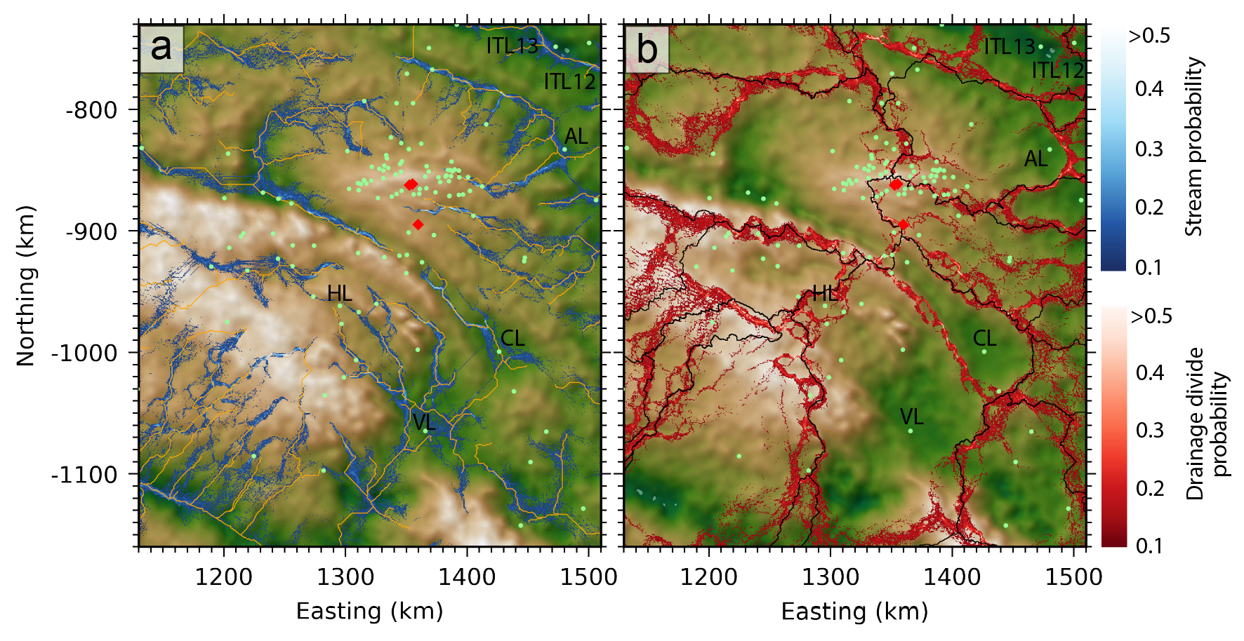
Figure 5 Subglacial drainage predicted using ensemble simulated beds. (a) Stream probability calculated from averaged stream predictions over the ensemble (blue), with predicted streams using Bedmap3 bed (orange). (b) Drainage divide probability calculated as averaged divides over the ensemble, with divides predicted using Bedmap3 (black). Ice cores also plotted (red diamonds) and radar-detected subglacial lakes (green points). Lakes with estimated minimum surface area >50 km² are labelled: AL = Aurora Lake (Tabacco et al., 2003); CL = Concordia Lake (Oswald and Robin, 1973); HL = Horseshoe Lake (Blankenship et al., 2009); ITL12+13 (Tabacco et al., 2003).

Concordia Lake is the largest subglacial lake within our study area, estimated from radar profiles to be minimum 45 km long and 16 km wide and containing water volumes of 200 ± 40 km³ (Tikku et al., 2005). Water inflow to this lake is well-constrained by the Concordia Trench, but outflow and downstream routing of released meltwater is not well-constrained by radar data. Our simulations suggest that water could drain either towards Vincennes basin or towards Adventure Trench, and the most probable drainage basin divides are to the southwest of the lake in contrast to the divides predicted using Bedmap3 grids (Fig. 5b). The lack of strong basal topographic control over downstream water routing suggested by limited available radar data indicates that downstream drainage could be sensitive to migrating ice divides, and more radar surveys are necessary to reduce the uncertainty in water routing.

The drainage basin constrained by the western Belgica Highlands and Concordia Ridge contains 11 subglacial lakes with a combined radar-estimated surface area of 147 km². Five of these lakes are located beneath thinner ice <3000 m along Concordia Ridge and 6 along the valley floor where ice can be over 3400 m thick. Our stochastic simulations constrain potential flow paths for a drainage system linking these lakes and indicate that large volumes of water draining from this basin could be routed either to the southwest similar to predictions using the Bedmap3 grid or 100 km further north (Fig. 5).

The preservation of deep ice layers in undisturbed stratigraphic sequence is sensitive to basal melt, ice flow, and basal ice accretion (Fischer et al., 2013; Van Liefferinge and Pattyn, 2013). Widespread subglacial lakes and meltwater drainage activity evidence basal melting in the Dome C region and poor hydraulic connectivity between lakes could increase potential for basal ice accretion, which together disturb deep ice stratigraphy and limit the preservation of old ice layers. For example, at Lake Concordia enhanced basal melting of 4.3 mm a⁻¹ ± 27 % is predicted over most of the lake, and 15.1 m ± 65 % of accreted ice in the northeast corner (Thoma et al., 2009). Careful consideration of the subglacial environment is required to identify targets for ice core drill sites and our uncertainty constrained subglacial drainage analyses identify sites with low potential for water ponding or drainage activity (Fig. 5a and b).

4.3 Geothermal heat flow

The GHF beneath Antarctica is largely unknown, however locally elevated GHF could impact basal conditions and ice flow especially beneath slow-flowing ice dome regions in the absence of frictional heat from basal sliding (Pittard et al., 2016). Ice sheet modelling investigations to identify suitable ice core drilling sites are also sensitive to GHF boundary conditions (Sutter et al., 2019). At Dome C, region-wide means range from 28.6 ± 5.1 to 59.0 ± 3.3 mW m⁻² in large-scale GHF models (An et al., 2015; Burton-Johnson et al., 2020; Hazzard and Richards, 2023; Lösing and Ebbing, 2021; Martos et al., 2017; Purucker, 2012; Shen et al., 2020; Stål et al., 2021), and 10's of kilometre scale spatial distributions differ significantly between models (Fig. 6). Local GHF estimates at the EPICA core site of 57.9 ± 6.4 mW m⁻² (Talalay et al., 2020) and 54.5 ± 3.5 (Passalacqua et al., 2017) have high uncertainties and might not reflect regional values.

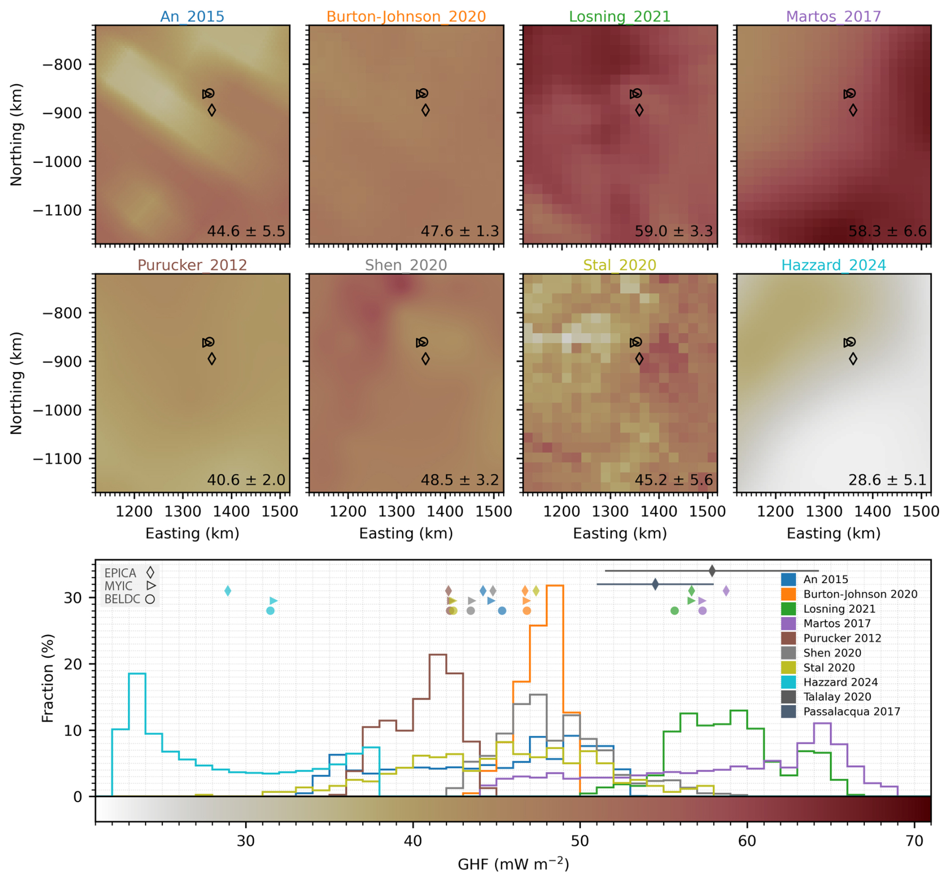
Figure 6 Geothermal heat flow (GHF) estimates near Dome C. Large-scale models plotted as native resolution in the upper 8 maps, with domain mean and standard deviation for each model provided in bottom right corner. Core sites plotted as EPICA: diamond, MYIC: triangle, BELDC: circle. Histograms for modelled GHF are plotted below, with associated value at core sites (diamonds, triangles, circles) together with other local GHF estimates and reported uncertainty at the EPICA core site.

Topographic focusing of geothermal heat can redistribute heat to local ridges or valleys, and the polarity of heat refraction patterns depends on the thermal conductivity contrast between ice and the underlying rock (Willcocks et al., 2021; Reading et al., 2022). The thermal conductivity of ice at depths beyond 750 m is estimated between 2.0–2.8 $\mathrm{W}{\mathrm{m}}^{-\mathrm{1}}{\mathrm{K}}^{-\mathrm{1}}$ (Willcocks et al., 2021), whereas igneous Antarctic bedrock ranges 1.5–4.0 $\mathrm{W}{\mathrm{m}}^{-\mathrm{1}}{\mathrm{K}}^{-\mathrm{1}}$ in samples limited to exposed outcrops mostly near the ice margin (Willcocks et al., 2025). The geology and corresponding thermal conductivity are uncertain beneath Dome C, so as an illustrative example of how topography could impact geothermal heat distribution we calculated an adjustment factor to account for local topographic modifications of background GHF following the simplified geostatistical approach of Colgan et al. (2021). Since the geology is not known, we adopt their globally averaged empirically determined averaging radius of 5 km and characteristic height needed to induce 100 % change in local GHF of 950 m, using their Eq. (2) to calculate potential magnitude and spatial patterns of heat redistribution. However, we recognise that the magnitude and polarity of such modifications could be substantially different in reality depending on the conductivity of the bed.

This calculation was done for each of the simulated beds in our ensemble to produce a topographic adjustment factor map, and Fig. 7a shows the ensemble median values. Similar to the ensemble elevation uncertainty, topographic adjustments to GHF are more consistent close to radar profiles, and the map inherently displays lower confidence adjustment factors closer to zero since topographic features far from data vary in location over the ensemble. Note that our confidence in adjustment factor is based only on uncertainty in bed geometry, and neglects uncertainty associated with bedrock thermal conductivity and polarity of thermal refraction, or the averaging radius and characteristic height parameters. Using our adopted parameterization of GHF redistribution, we show that locally elevated GHF up to 30 % more than the background value could occur within the troughs (e.g. Adventure, Concordia), yet along ridges (e.g. Concordia) local GHF could be 30 % lower (Fig. 7a and b). Beneath the Dome Fuji ice dome, topographic modification to background GHF was predicted to induce widespread local anomalies of ±20 %, aggregating to raise the regional average by 0.6 % (Shackleton et al., 2023). The Dome C regional mean values are low over the ensemble at 0.05 % ± 0.04 %, though regional standard deviations of 0.1 % ± 0.0 % indicate widespread potential for localised GHF adjustments of 3–7 mW m⁻² based on modelled range ca. 30–70 mW m⁻².

Figure 7 Topographic adjustments to geothermal heat flow (GHF). (a) Local topographic adjustments to GHF displayed as the median adjustments over the ensemble of 100 simulated bed elevation grids. Ice thickness contours at 500 m intervals are drawn in black. (b) Enlarged view of the central plateau near the ice core sites, also with radar-inferred subglacial lakes drawn as green points. (c) Histogram of topographic adjustments, with ensemble median sampled adjustments at the subglacial lake sites (green) and core sites (orange) with median absolute deviation error bar.

We find 80 % of the radar-inferred subglacial lake sites are within a zone of locally elevated GHF (Fig. 7c), suggesting that topographic modification of geothermal heat could be a contributing factor to the spatial pattern of basal melting and lake distributions in regions where basal ice is close to the pressure melting point. Spatial variability in GHF at much larger scale of 10's of kilometres increased modelled basal melt rates in the Aurora Basin by up to 4.5 % (McCormack et al., 2022). Smoothed bed in data sparse regions of previous interpolations therefore limits robust assessments of basal thermal conditions, and using realistically rough topography should be prioritized when delineating thawed/frozen basal ice and calculating melt rates, which will also improve the reliability of basin-wide thermodynamical and ice flow modelling. Given the large uncertainties and range of modelled GHF near Dome C and across Antarctica, the local topographic adjustments to GHF could be used instead to find suitable sites for future ice coring, prioritising sites with locally lowered GHF. Our analysis shows that the EPICA core site could be situated in locally elevated GHF by 2 % (Fig. 7c), whereas the new sites BELDC and MYIC are situated in a region with potentially lowered GHF by 12 %–13 % which could be favourable for deep ice layer preservation. Considering the impacts of uncertain bed geometry alone, variability over the ensemble is less than 0.08 % for all ice core sites since they are generally close to radar data. Borehole GHF estimates should also be adjusted to account for the potential range of local topographic modifications before extrapolating over a larger region.

5 Conclusions

New airborne radar surveys uncover previously unmapped sectors of the Belgica Highlands, and we used a rigorous approach to integrating new observations with available ice thickness data near Dome C. Our measurement compatibility analysis guided strict filtering procedures, and we find that rigorous quality screening and cross-validation to integrate new measurements with existing data is crucial for characterising basal roughness. This process is a necessary pre-requisite for reliable gridding or simulating of bed topography to minimize the impact that nearby inconsistent measurements have on spatial statistics. Our simulated bed has improved representation of basal roughness in data sparse regions, with region-wide means more than double those of previous work and spatial patterns free from the influence of radar survey geometry. The ensemble simulation approach for mapping elevation uncertainty accounts for the combined influence of data density and local bed roughness characteristics, producing higher uncertainties where measurements are sparse and the terrain is rough. Domain-mean bed elevation uncertainty is 53 m and reaches 260 m in data-sparse regions, however, near the BELDC and MYIC ice core sites dense radar coverage constrains elevation uncertainty effectively to zero at a 500 m grid scale.

Subglacial drainage analyses using ensemble simulated bed identify well-constrained drainage away from the Dome C Plateau, but poorly constrained outflow from Concordia Lake and western Belgica Highlands drainage basin. These uncertainties impact predictions of subglacial lake connectivity and downstream water transport, highlighting locations where additional radar surveys are required to adequately constrain subglacial drainage. Our work also reveals potential patterns of local topographic modifications to regional GHF, which could be critical to delineating thawed/frozen bed, locating suitable sites for ice core drilling, and interpreting retrieved cores and borehole measurements/modelling investigations. We identify locations where local bed topography could lower GHF by up to 30 % of the regional value, and the MYIC and BELDC ice core drilling sites are within a zone of locally lowered GHF by 12 % which could be favourable for preserving deep ice layer continuity. Topographic focussing of geothermal heat could enhance basal melting in many trough locations and exert a control over the distribution of subglacial lakes; our analysis shows most radar-inferred subglacial lakes occurring in a region where we predict locally elevated GHF. Given the large spread among continental-scale GHF models, we suggest that locally resolved topographic adjustments to GHF provide an independent and complementary constraint on spatial variability in basal conditions.

Our study emphasizes that the physical realism of Antarctic subglacial boundary conditions depends on capturing the inherent variability and anisotropy of the bed. These properties are currently obscured in widely used Antarctic bed products due to smoothing from isotropic deterministic interpolation, which limits their reliability for use in ice-sheet and subglacial environment modelling. Survey design should capture directional anisotropy by acquiring profiles along multiple azimuths, extending beyond traditional along- and across-flow transects, while gridded products should prioritize simulation-based approaches that maintain realistic spatial continuity in data-sparse regions. By resolving variability at scales relevant to basal processes and adopting ensemble-based topography, the community can more effectively propagate measurement and interpolation uncertainties into subsequent ice-sheet and subglacial environment analyses.

Appendix A

Figure A1 Consistency between individual radar surveys and all other surrounding data. Each figure panel shows a map with 50 m radius crossover points as an X coloured according to the difference in value (Red-Blue colormap). Survey track is shown as a grey line and all other survey tracks are shown as yellow lines. The adjacent histograms show the differences in value between each intersecting survey as a probability density function, with the upper plot showing detailed differences within ±150 m and lower plot showing the full range of crossover differences. A legend for the histograms is shown to the right with some summary statistics for overall differences between the survey and surrounding measurements.

Table A1 Radar-derived ice thickness datasets used. BAS = British Antarctic Survey, BE-OI = Beyond EPICA Oldest Ice, KOPRI = Korea Polar Research Institute, UA = University of Alabama, DTU = The Technical University of Denmark, CPH = University of Copenhagen, AWI = Alfred Wegener Institute, AAD = Australian Antarctic Division, INGV = Istituto Nazionale di Geofisica e Vulcanologia, UTIG = University of Texas Institute for Geophysics, NASA = National Aeronautics and Space Administration, PRIC = Polar Research Institute of China, LDEO = Lamont Doherty Earth Observatory, CReSIS = Center for Remote Sensing of Ice Sheets.

^∗ All surveys had data filtered out within 0.6 km of crossover sites if differences were >50 m, with priority determined by mean absolute differences between all other surveys.