Linking the evolution of floe sizes to the sea-ice deformation history using SAR imagery

Arctic sea ice is a mosaic of ice floes whose distribution, sizes, and thicknesses greatly impact the interaction of sea ice with the atmosphere and the ocean. However, we are still lacking knowledge of the physics to describe the complex interplay of ice floes that are a key characteristic of sea ice. Here, we outline a framework to characterize sea-ice deformation at the floe-scale from observational data by studying the mechanical interactions of multiple identifiable floes. We use Sentinel SAR imagery acquired during the MOSAiC expedition to map ice floes in the larger area around Polarstern and describe the floe-size distribution with floe diameters from tens of kilometers down to tens of meters. We present a new chord-based mapping of the floe-size distribution using a new numerical statistical conversion between floe chord and size distribution based on observed floe geometries. With the repeated coverage of SAR imagery, ice motion is tracked and deformation estimates between consecutive SAR images are derived. By combining both floe-size estimates and deformation rates we provide insights into how the floe composition changes in regions that were exposed to deformation. To do so, we subdivide the SAR images into 50 × 50 km boxes and study how the floe-size distribution evolves as a function of divergence rates on a daily time scale. We find clear signatures of fracturing into smaller floes for both divergent and convergent ice regimes. The observed mechanical redistribution of floe sizes is described by a power-law that steepens with increasing divergence rate. Our observational-based process study is the first to show that internal ice fracture could be a primary driver of the power-law form of the floe-size distributions. Finally, we present a parameterization for the mechanical redistribution of floe sizes in fracture events for large-scale continuum sea-ice models with an interactive subgrid-scale floe-size distribution.

1 Introduction

The Arctic and Antarctic sea ice cover is formed by a mosaic of pieces of ice referred to as floes. These floes are observed over a wide range of scales and their relative abundances in a region are described by the floe-size distribution (FSD). In the context of this study, the FSD describes the number of floes of a certain size abundance in a control volume. Overall, three groups of processes drive the evolution of the FSD: thermodynamics, interaction with ocean surface waves, and mechanical fracture from horizontal ice deformation; at the same time, the FSD feeds back on each of these processes and thereby modulates the mechanical, thermodynamic, and dynamical behavior of sea ice. Besides lateral melting and freezing along floe edges, which alters the sizes of floes, thermodynamic processes also include the welding of multiple floes in freezing conditions and new ice formation as either pancake or nilas. Ocean swell propagating into the ice cover or surface waves induced by wind in open water patches within the ice cover bend and break floes, resulting in a complex coupled interplay between FSD modulations and dampening of wave spectra. Lastly, when wind and ocean currents exert stresses on the ice cover that exceed the ice strength, failure and fracture of the ice cover result in smaller floes (henceforth known as internal fracture of floes). Depending on ice concentration and distance to the ice edge these three major process groups have different importance leading to differing balances between the processes for different regions and seasons. In the marginal ice zone, characterized by unconsolidated ice and direct ocean influence, the FSD depends on wave interaction and thermodynamic processes. In the more consolidated pack ice, the effect of wave interaction is negligible and thermodynamics and internal fracturing determine the FSD.

To incorporate these floe-scale processes in numerical sea ice models, an FSD within each grid cell of a model has been defined. The evolution of the FSD is driven by parameterizations of the processes mentioned above with varying degree of details (e.g. Zhang et al., 2016; Roach et al., 2018). To date the most complete implementation of an FSD is in the Los Alamos sea ice model CICE presented by Roach et al. (2018, 2019), which is based on a joint floe-size and thickness distribution (FSTD, after  Horvat and Tziperman, 2015). Its formulation includes all relevant thermodynamic processes: lateral melting and freezing, welding of floes in freezing conditions, and ice formation as pancake or nilas (depending on wave spectra). In addition, the model employs complex wave-interaction schemes describing the fracturing of floes in response to the ice bending between wave crests. Coupled to a wave model, Roach et al. (2019) simulated the interactive feedback between wave induced floe fracture and wave attenuation that shapes the marginal ice zone. In addition to thermodynamics and wave interaction, Horvat and Tziperman (2015) presented a parameterization of fracture and deformation induced mechanical redistribution of floes sizes based on the redistribution scheme for the ice thickness distribution (Thorndike et al., 1975) with additional, more complex assumptions. This scheme was neglected in Roach et al. (2018) due to its complex formulation with no observational data available at that time backing its theory. Therefore, in the current version of CICE, internal deformation does not affect the simulated FSD.

This leaves the current model formulation tailored towards simulating the complex interactions in the marginal ice zone, where all important processes are included. Using floe observations based on satellite altimetry data, Horvat et al. (2019) evaluated the model performance and found decent agreement of the representative floe radii in the marginal ice zone. In the consolidated pack ice, however, where the effect of waves is limited, the model strongly overestimates floe sizes (Horvat et al., 2019; Roach et al., 2019), because no process actively balances the welding of floes resulting in an accumulation of floes in the largest size bin. To counteract this accumulation, Bateson et al. (2022) proposed a simple FSD restoring scheme for brittle fracture that relaxes the prognostic FSD to a power-law distribution with a predefined exponent. While better agreement with satellite-based FSD observations was reported, the restoring scheme is independent of internal deformation, leading to a constant redistribution of floes from larger to smaller bins until the predefined power-law exponent is reached, even in dynamically “calm” conditions with no internal deformation. Observations, however, show that ice fracture is strongly spatially localized and intermittent, motivating us to develop a parameterization that fractures and mechanically redistributes floes directly dependent on internal deformation simulated by the dynamical ice model.

In this study, we present concurrent floe size and deformation estimates from SAR-images to study the impact of fracture on the evolution of floe sizes from an observational perspective. We introduce a new deformation-informed ice classification of SAR backscatter and statistical approach to measure the floe size distribution in consolidated winter pack ice conditions. This work is based on Sentinel-1 acquisitions over the MOSAiC expedition (Nicolaus et al., 2022) providing us with a 2.5 month period of continuous observations from March till May 2020. We subdivide the SAR images into smaller subregions with a size comparable to a CICE grid cell (50×50 km²) and track these with the ice motion. By linking the evolution of the FSD within each subregion to the observed deformation of the subregion, we develop a parameterization of mechanical FSD redistribution based on observed divergence.

2 Satellite data

This study is based on sequential SAR scenes captured in HH polarisation Extra Wide swath mode, sourced from the Sentinel-1 mission by the European Space Agency (ESA). In our study the SAR images serve a dual purpose: firstly, to extract ice drift and deformation, and secondly, to differentiate ice and open water presence and identify floes and measure their sizes. We select SAR images along the drift path of the MOSAiC expedition (Nicolaus et al., 2022), covering the area within approximately 150 kilometers of the research vessel Polarstern, for two reasons: (1) a processed Lagrangian drift dataset at sub kilometer resolution based on these images is already available (von Albedyll and Hutter, 2023), and (2) the wealth of observational data acquired during the expedition that can be used for validation and contextualization. The images were acquired between March 13 and 31 May 2020, at daily intervals, following the drift of RV Polarstern during the MOSAiC expedition through the central Arctic and the region North of Fram Strait. The images cover approximately 400 × 400 km² with a spatial resolution of 50 m. The spatial coverage of the SAR scenes used is shown in Fig. A1. The backscatter information of the images is used to classify ice and open water to measure floe sizes.

As we are interested in the FSD redistribution induced by ice fracture, we require the FSD information in consecutive images as well as the ice drift and deformation between those images. The ice drift between consecutive SAR images was previously calculated with a feature tracking method for the MOSAiC campaign (Krumpen et al., 2021). The algorithm of Thomas et al. (2008, 2011) and Hollands and Dierking (2011) was applied to HH-polarized Sentinel-1 scenes with a 50 m pixel resolution and a typical temporal spacing of 1 d, yielding drift fields on a regular 700 m grid from which divergence, convergence, and shear were computed as spatial derivatives. The complete dataset for SAR-derived ice drift and deformation is available at von Albedyll and Hutter (2023). With this drift information we track the motion of ice between consecutive images, and determine deformation rates that can be linked to the observed changes in floe sizes as well as serve as an additional input to our open water classification.

We validate our SAR-based classification of ice and open water with the sea ice freeboard product ATL10 from the ICESat-2 satellite altimeter (Kwok et al., 2023). Following a methodology akin to Petty et al. (2021), we detect leads within the ice cover using the freeboard and surface classification data of ATL10. Subsequently, we extract ICESat-2 data that coincide with our SAR image coverage and perform a drift correction using the SAR derived drift information to account for ice displacements between different acquisition times. In overlapping regions, we use the detected leads to compute reference floe chord distributions (FCDs) to assess the accuracy and reliability of our SAR-based ice and open water delineation.

For the statistical conversion of floe chords to floe sizes, we study the geometry of floes in detail using two published floe data sets. The first has floes identified manually in a MEDEA image of the Beaufort Sea on 8 July 2014 (Stern et al., 2018a). At a resolution of 1 m, the image contains 6002 floes of sizes between 1 m and 2.4 km, and all floe shapes are provided in shape files. A second data-set of automatically tracked floes in MODIS images (Lopez-Acosta et al., 2019; Lopez-Acosta and Wilhelmus, 2021) contains 28 611 floes of sizes 4.9 to 85 km. Floe shapes are provided as binary images of 250 m and the data span the entire Arctic from 2003 to 2019 covering the months April to August.

3 Data processing

The primary objective of our study is to investigate how the fragmentation of the ice cover resulting from internal deformation changes the distribution of floe sizes. This fracture and deformation predominantly occurs within consolidated ice floes, primarily in pack ice under freezing conditions in winter. Focusing on these consolidated conditions, we extract a period of the MOSAiC expedition in this study, where RV Polarstern was located far away from the marginal ice zone to exclude wave effects. Because thermodynamic effects on floes act on longer time scales, we isolate the effect of sea-ice dynamics by only studying changes in the floe size distribution over short time periods. The focus on consolidated ice poses a significant challenge on the delineation of sea ice floes, as floes often are in contact, making the boundaries between floes appear ambiguous. Most previous studies of the FSD have focused on summertime conditions or the marginal ice zone, with much lower ice concentration allowing a floe to be defined as a piece of ice surrounded by open water (e.g. review article by  Stern et al., 2018b). While an ideal floe boundary definition would entail zero or reduced ice strength, this parameter cannot be directly observed from satellite or aerial imagery. When winds and vulnerabilities in the ice align to force the active deformation of ice, discontinuities in ice drift patterns may offer means to delineate floes. However, delineating floes by deformation is limited to the sporadic times when deformation occurs and by the coarse resolution of drift estimates derived from SAR images (∼ 1 km). Therefore, we chose to consider open water and leads as boundaries derived from the SAR backscatter to define floes, which allows us to study floe sizes down to the resolution of the SAR imagery (whose pixels are 50×50 m²). Here, we use a statistical approach to account for the impact of floe contact on the computed FSD, which is described in full length in Sect. 3.2.1 and 3.2.4. Our definition of floes as areas surrounded by open water is also supported by the current emphasis in CICE on utilizing floe size distribution to influence thermodynamic processes, such as lateral melt, ensuring consistency over the whole range of ice regimes.

The overall aim behind our analysis is to describe a parameterization of the deformation induced changes of the floe size distribution in numerical sea ice and coupled climate models. Therefore, we aim to study these changes at a spatial scale similar to the resolution of current climate models. To do so, we compute these changes in 50×50 km² squares, which we refer to henceforth as the region of interests (ROIs). Our overall procedure is the following: we subdivide the first of the subsequent SAR images into multiple ROIs. We use the backscatter of the SAR image to distinguish ice and ocean and compute the floe size distribution within the ROIs. Next, we use the drift information to compute the position of the ROIs in the second SAR image, where we also compute the FSD. From the distortion of the ROI boundaries after advection, we derive the deformation rates associated with the overall deformation of the ROI and link that to the observed changes in the FSD. Combining all ROIs we are able to study how the change in FSD depends on the deformation rates and outline a parameterization of this feedback.

The outlined analysis poses three major challenges that we describe in depth in the following data processing section: (1) The classification of ice and open-water in SAR images, where we develop a deformation informed thresholding method of the SAR backscatter. This method allows us to classify each pixel of the SAR image as either ice or ocean resulting in an ice-ocean mask used to determine the FSD. (2) The measurement of floe sizes in wintertime pack ice conditions, which is hindered by frequent floe contacts in consolidated ice. To overcome the difficulty of identifying individual floes, we extract randomly oriented lines from the ice-ocean mask and measure the lengths of ice segments between the ocean breakpoints, so called floe chords. Based on the geometry of observed floe shapes, we statistically convert these chord lengths into floe size estimates. (3) Finding a relation of changes in the floe size distribution with ice fracture, which is a nonlinear chaotic process strongly dependent on ice conditions and forcing. Here, we aim to extract a general functional relationship by averaging over many ROIs with similar deformation rates. In the following sections, we describe the individual processing steps in detail and present solutions to the aforementioned challenges.

3.1 Ice-water classification

SAR satellites are valuable for observing the Arctic sea ice because they offer high resolution, day-and-night coverage, and penetrate clouds. Hence, their images are a major source for ice charting. The main disadvantage of SAR images, however, is the ambiguity of the acquired backscatters signal, requiring experienced analysts to identify different ice types and open water (Scheuchl et al., 2004; Dierking, 2013), often at resolutions much coarser than the image resolution. Automated ice classification of SAR images has been an active field of research for the past two decades (Zakhvatkina et al., 2019). Modern machine-learning based classifications aim to distinguish several ice classes based on ice age, thickness, and degree of deformation, as well as distinguishing various lead and open water types. Many different methods have been proposed (e.g. Ressel et al., 2015; Lohse et al., 2020; Kortum et al., 2024), but to date no comprehensive comparison and evaluation has been presented and no standard method has been established. Since our task at hand is simpler and limited to distinguish only the two classes of ice and open water, we decide to primarily use the backscatter signal to separate them. Depending on the incidence angle (the angle between the radar beam and the surface normal), open-water can appear brighter or darker than ice in SAR images (Lohse et al., 2020). In our study period and region, lead fractions are consistently well below 5 % in multiple satellite products (von Albedyll et al., 2024). Therefore, the SAR images in our analysis are mostly covered by ice, with only limited open water in leads. Thus, the mode of backscatter in a subdomain of the image (where variability in the incidence angle is negligible, e.g. in a 50×50 km² ROI) can be regarded as the typical backscatter of an ice surface for the given incidence angle at that position. Similarly, the standard deviation of the backscatter in this subdomain represents the spread in ice backscatter values. When the backscatter deviates from the average ice value of the subdomain by multiple orders of magnitude, it is unlikely that it originates from an ice surface and we classify the pixel as a lead, i.e. ocean. For this classification, the standard deviation and modal backscatter of the area surrounding each pixel are required, which we obtain by computing both in a window moving over the entire image. With the moving window, we also account for the varying backscatter signal of different ice types found in the image. In the study period, open water is only formed by deformation, as significant melting does not occur due to the cold temperatures. Therefore, we dynamically lower the thresholds in regions of divergence and shear (shear must be high to have an appreciable effect) motion. Finally, we manually tune the thresholds for each image individually to optimizing the open water classification visually (optimized parameters are provided in the associated code repository Hutter, 2026a).

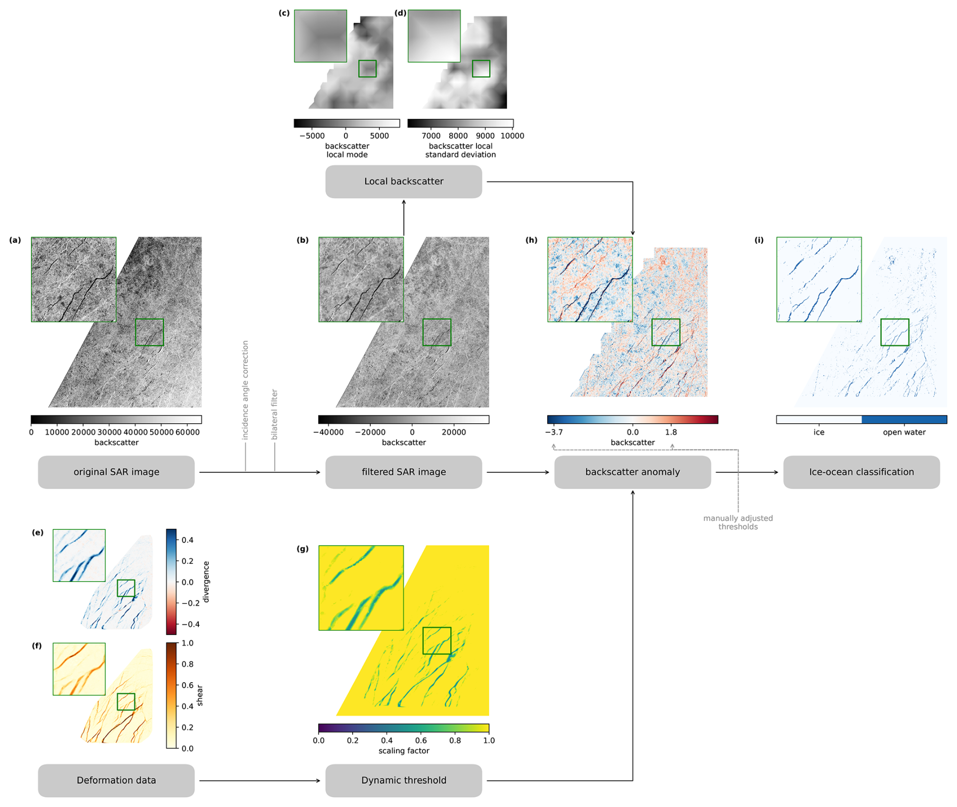
Figure 1 Processing pipeline to generate ice-ocean mask from SAR images and SAR-derived drift.

In the following, we describe in detail the individual processing steps, starting with the original SAR image and ending with the ice-ocean classification (generating the so-called ice-ocean mask), as illustrated in Fig. 1. First, we use a bilateral filter to remove the speckle noise in the backscatter, similar to Hwang et al. (2017), and corrected for the varying incidence angles over the image (Fig. 1b). Next, we compute the mode $\widehat{I}(x,y)$ and standard deviation σ_I(x,y) of the backscatter signal over a moving window of size (50×50 km² or 1000×1000 pixels, respectively), which we henceforth refer to as running mode or running standard deviation. To reduce computation costs, we do not shift the moving window pixel by pixel to compute a true running mode, but shift the window by 500 pixel each step to compute the mode and standard deviations at anchor points resulting in half overlapping 1000×1000 pixel boxes. To obtain local backscatter mode and standard deviation at all pixels of the SAR image, we bilinearly interpolate these values from the anchor points (Fig. 1c, d). The region size was set to be large enough to average out the effect of lead systems on the standard deviation. Also, the divergence ${\dot{\mathit{ϵ}}}_{\mathrm{I}}=\frac{\partial u}{\partial x}+\frac{\partial v}{\partial y}$ and shear rates ${\dot{\mathit{ϵ}}}_{\mathrm{II}}=\sqrt{{\left(\frac{\partial u}{\partial x}-\frac{\partial v}{\partial y}\right)}^{\mathrm{2}}+{\left(\frac{\partial u}{\partial y}+\frac{\partial v}{\partial x}\right)}^{\mathrm{2}}}$ are computed from the drift product and interpolated bilinearly to each SAR pixel (Fig. 1e, f).

Also, the divergence ${\dot{\mathit{ϵ}}}_{\mathrm{I}}$ and shear rates ${\dot{\mathit{ϵ}}}_{\mathrm{II}}$ of the drift product are interpolated bilinearly to each SAR pixel (Fig. 1e, f). From the interpolated deformation rates we compute a scaling factor s(x,y) to reduce the threshold as follows,

$$\begin{array}{}\text{(1)}& {\displaystyle }{s}_{\mathrm{I}}(x,y)=max\left(\mathrm{0.5},min\left(\left({\dot{\mathit{ϵ}}}_{\mathrm{I}}\right(x,y)-\mathrm{0.5}{\mathrm{d}}^{-\mathrm{1}})/\mathrm{0.45}{\mathrm{d}}^{-\mathrm{1}},\mathrm{1}\right)\right),\text{(2)}& {\displaystyle }{s}_{\mathrm{II}}(x,y)=max\left(\mathrm{0.5},min\left(\left({\dot{\mathit{ϵ}}}_{\mathrm{II}}\right(x,y)-\mathrm{1.0}{\mathrm{d}}^{-\mathrm{1}})/\mathrm{0.5}{\mathrm{d}}^{-\mathrm{1}},\mathrm{1}\right)\right),\text{(3)}& {\displaystyle }s(x,y)=max\left(\mathrm{0.5},min\left(s_{\mathrm{I}}\right(x,y)\times s_{\mathrm{II}}(x,y),\mathrm{1})\right),\end{array}$$

which are the independent scaling factors for divergence and shear and their product is a joint scaling factor. Note that the scaling coefficient is capped by 0.5 and 1 for divergence and 0.75 and 1 for shear, such that the threshold is at most halved by the dynamic thresholding and does not automatically yield to an open-water classification of deforming pixels. The spatial variation of the resulting scaling factor is shown in Fig. 1g. In the next step, we compute the local backscatter anomaly, which describes the difference of the backscatter pixel value to the local backscatter mode in relation to the scaled local standard deviation,

$$\begin{array}{}\text{(4)}& I_{\mathrm{a}}(x,y)={\displaystyle \frac{I(x,y)-\widehat{I}(x,y)}{s(x,y){\mathit{\sigma }}_I(x,y)}}.\end{array}$$

We identify pixels as open water if the backscatter anomaly is below a lower threshold $I_{\mathrm{a},min}$ or exceeds an upper threshold $I_{\mathrm{a},max}$. These thresholds were manually adjusted for each image to optimize the ice-ocean mask with the exact values documented in Hutter (2026a). As part of this manual adjustment also the deformation rate thresholds and scaling magnitudes in Eqs. (1)–(3) were tuned, where the same thresholds were used for all images. In a last step, we apply a linear filter to the generated ice-ocean mask to damp noise at the pixel level (Ringeisen et al., 2023; von Albedyll et al., 2024), assuming that open water should be mainly found along leads in long and narrow strips rather than isolated openings in the ice cover. We apply a rotating linear kernel of length 7 at each pixel and determine the orientation of the lead as the kernel orientation with the lowest standard deviation. Along this orientation the ice ocean mask is averaged with the same linear kernel. We only classify pixels as open water if the filtered value is higher than 0.75 (Fig. 1i). The filter maintains open water points connected in lines and reduces the noise at the grid-scale speckle. The performance of this ice-ocean classification and potential misclassification of bright pressure ridges or frost flowers will be assessed and discussed in Sects. 3.4 and 5.

3.2 Wintertime floe-size measurements in SAR imagery

To date, satellite or airborne imagery in the visible spectrum are the major source of floe size and shape data (e.g. Rothrock and Thorndike, 1984; Toyota et al., 2011). Therefore, these studies were limited by natural illumination and mostly represent broken-up summer sea ice conditions with lower ice concentrations (Stern et al., 2018b). In these conditions, bright ice and dark ocean can easily be classified and subsequently different methods are used to delineate individual floes in the ice cover. While floes were first identified manually (Rothrock and Thorndike, 1984), recent methods are almost fully automated (Gherardi and Lagomarsino, 2015; Lopez-Acosta et al., 2019; Denton and Timmermans, 2022). Hwang et al. (2017) presented a semi-automated approach to identify floes in SAR images. Despite the availability of SAR images during the Polar night, their algorithm has been applied to images of summer sea ice only. In consolidated ice conditions, as found in wintertime pack ice, floes can be in partial or complete contact with other floes and therefore are not necessarily surrounded by open water, which challenges the segmentation step of these algorithms, leaving us with no floe data from visible or SAR imagery for winter time. Horvat et al. (2019) and Petty et al. (2021) have used satellite altimetry to measure the length of ice segments, so-called floe chords, along the satellite track to study winter time floes. Floe chords are one proxy for floe sizes, in addition to floe area, perimeter, or mean caliper radius (Rothrock and Thorndike, 1984). The main advantage of using floe chords is that they can be measured directly on the ice-ocean mask without identifying floes directly in an image. The FCD and FSD are related by statistics if the floe geometry is known, which we discuss in the following section. To cope with the consolidated ice conditions in our SAR images, we will use a floe chord proxy. We present a new approach of measuring the FCD and perform a statistical conversion to compute the FSD that is described in detail in the following. The development of this statistical conversion includes an in-depth study of floe geometries.

3.2.1 Floe chord measurements

In the literature floe chords have been mainly measured in altimetric satellite data where no two-dimensional (2D) information was available and typically one chord per floe is sampled (Horvat et al., 2019; Petty et al., 2021). Satellite images in our analysis, however, hold 2D information and by sampling the image over multiple directions we are able to sample multiple chords from the same floe. If the geometry of the floe is known, this dense sampling allows us to reverse engineer the size of floe from the sampled chords. In this section, we introduce the method of how we sample floe chords for a subdomain of an image and how many samples are required for a representative estimation of the FCD.

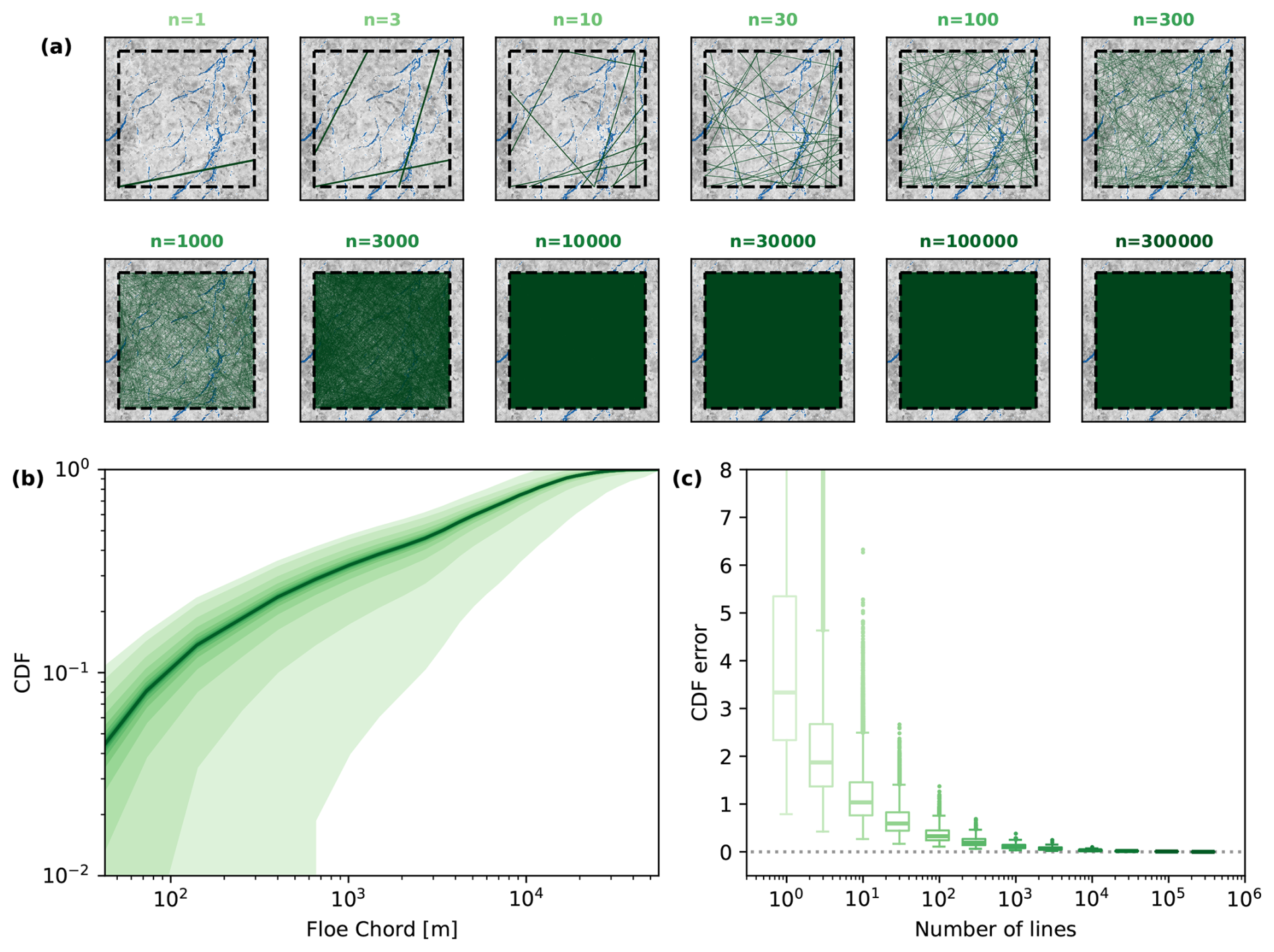
Figure 2 Illustration of the floe chord sampling strategy applied in our analysis. Panel (a) shows for an example ROI of the SAR image from 14 March 2020 how the coverage of the sampling increases with increasing number of randomly drawn lines to measure chords. Panel (b) illustrates how the cumulative FCD varies with increasing number of sampling lines. For each number of lines the cumulative FCD is presented as a shaded area of the mean plus/minus one standard deviation. The color coding of the number of lines is provided in panel (c) using the same color scheme. Panel (c) shows the variation of the cumulative FCD error for each sampling size as a boxplot. The cumulative FCD error is defined as the cumulative absolute differences between the subset cumulative FCDs and the full cumulative FCD of all 300 000 sampling lines.

To determine the FCD of a 50×50 km² (1000×1000 pixels) ROI, we draw random lines through the ROI by selecting two random points on two different faces of the boundary of the ROI for each line. We extract the ice-ocean mask information for all points on the line and measure the length of all ice segments separated by ocean pixels, which are considered floe chords along this line. Note, that we also consider the first and last segment as valid chords, even if the segment is cut short by the ROI boundary. We repeatedly draw new lines and accumulate the chords into a distributions, until the FCD converges. Figure 2 illustrates an example region of how the FCD converges with increasing numbers of random lines, up to 300 000. Next, we study how the spread in cumulative FCD for subsets of these 300 000 lines varies with the size of the subset. To do so, we define different subset sizes, split the 300 000 lines accordingly, and compute the cumulative FCD for each subset. Figure 2b shows that the spread in the cumulative FCDs for each subset decreases quickly with increasing number of lines. For more than 10 000 lines, which is roughly where the entire ROI is covered with lines (Fig. 2a), the cumulative FCD is converged and the cumulative FCD error becomes constant. The cumulative FCD error is defined as the sum of the absolute difference over all bins between the cumulative FCD of the subsets with the converged cumulative FCD of all 300 000 lines (Fig. 2c). Based on these findings, we choose to draw 30 000 lines for each ROI in our analysis to ensure a sufficiently converged FCD.

3.2.2 Statistics of floe chord to floe size distributions

In this section, we summarize how the distributions of floe chords and floes sizes are related by Bayesian statistics. Our derivation follows Rothrock and Thorndike (1984) and Horvat et al. (2019). We define the floe size d as the diameter of a circular floe of the same area. Floe chords are denoted by c. Bayes' theorem relates both floe size and chord distributions as

$$\begin{array}{}\text{(5)}& F(d;c)S\left(c\right)=\stackrel{\mathrm{̃}}{F}(c;d)P\left(d\right),\end{array}$$

where S(c) is the FCD and P(d) is the FSD, both defined as probability density functions. F(d;c) is the conditional probability where F(d;c)dd describes the probability that floes of size d to d+dd were sampled given that we measure the floe chord c. Respectively, $\stackrel{\mathrm{̃}}{F}(c;d)\mathrm{d}c$ is the conditional probability to measure floe chords of c to c+dc given that a floe of size d is sampled. While F(d,c) is unknown and by itself depends on the FSD, we can determine $\stackrel{\mathrm{̃}}{F}(c;d)$ by splitting it into a combination of a geometrical problem and a sampling probability,

$$\begin{array}{}\text{(6)}& \stackrel{\mathrm{̃}}{F}(c;d)=G(c;d)H\left(d\right),\end{array}$$

where G(c;d) describes the probability of measuring a floe chord c given that a randomly drawn line hits a floe of size d and H(d) is the probability that a floe of size d is sampled by a randomly drawn line (Rothrock and Thorndike, 1984). By definition, the integral of the conditional probability F(d;c) over floe size d equals one. By integrating Eq. (5) over the floe size d we obtain,

$$\begin{array}{}\text{(7)}& S\left(c\right)=\underset{\mathrm{0}}{\overset{\mathrm{\infty }}{\int }}\stackrel{\mathrm{̃}}{F}(c;d)P\left(d\right)\mathrm{d}d=\underset{\mathrm{0}}{\overset{\mathrm{\infty }}{\int }}G(c;d)H\left(d\right)P\left(d\right)\mathrm{d}d.\end{array}$$

This equation allows us to compute the FCD provided that we know the FSD and details of the floe geometry. Assuming circular floes, Rothrock and Thorndike (1984) presented an analytical description of this relationship and more importantly also derived its inverse – how to compute the floes size distribution from floe chords – using the Abel integral transform. Multiple studies, however, have shown that the floes are not circular but have more complex shapes (e.g. Rothrock and Thorndike, 1984; Toyota et al., 2011; Gherardi and Lagomarsino, 2015). In the next section, we present an in-depth analysis of observed floe geometries to find a G(c;d) for realistic floe shapes and study if these geometrical properties are scale invariant over different floe sizes to allow for an inverse computation of the FSD.

3.2.3 The geometry of floes

In this section, we study the geometry of ice floes to determine the conditional probability G(c;d) that can be used in the floe chord and size conversion Eq. (7). Besides finding G(c;d), we are also interested if G(c;d) is scale invariant, i.e. $G(c;d)=d\stackrel{\mathrm{̃}}{G}\left(\frac{c}{d}\right)$. Previous studies of different proxies of floe geometry have shown scale-invariance (e.g. Toyota et al., 2011). Once G(c;d) is known and is confirmed to be scale invariant, we can transfer Eq. (7) to an inverse linear problem and compute FSDs from measured FCDs.

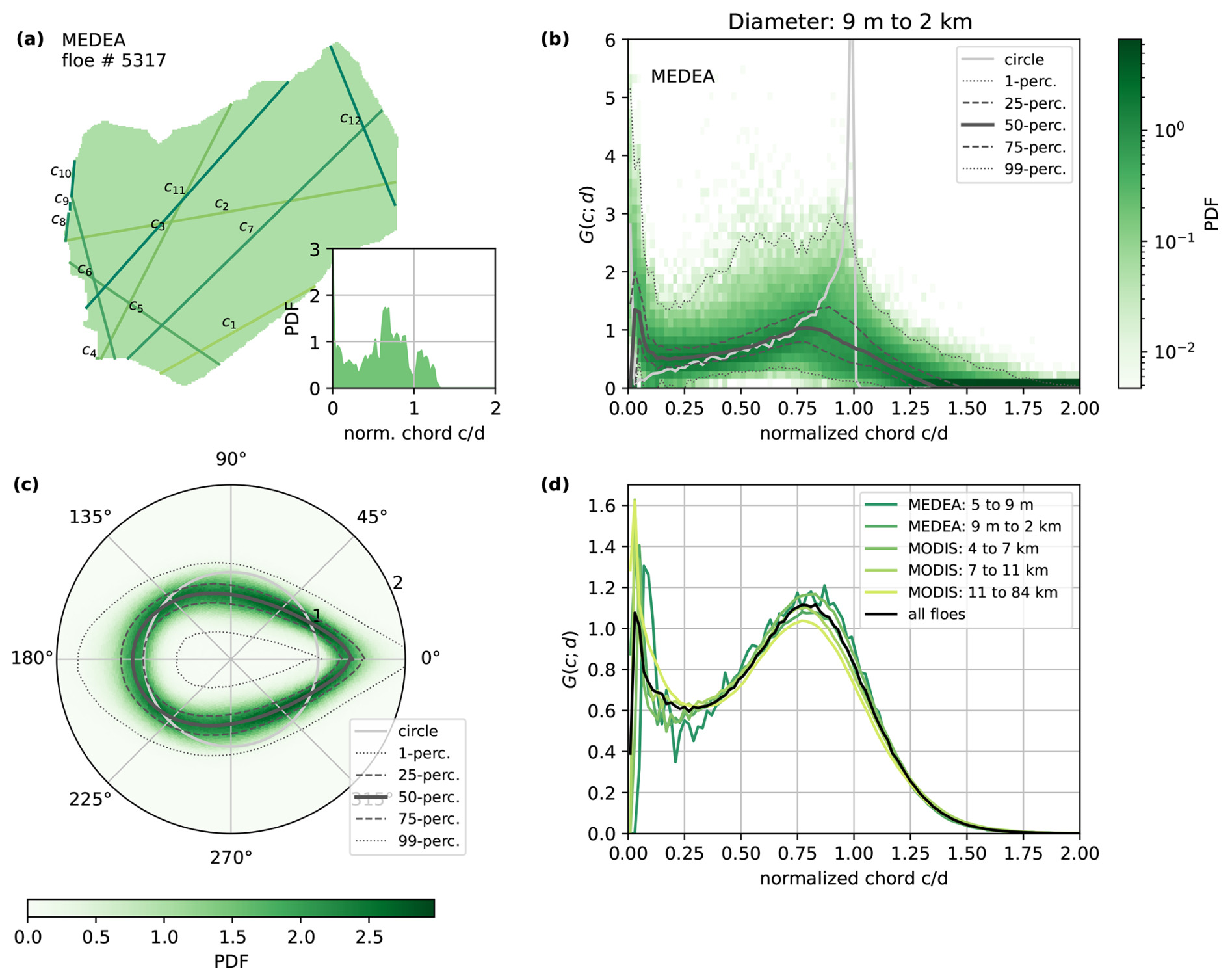
Figure 3 Aspects of floe geometry based on 34,613 observed floe shapes. Panel (a) shows one example floe (No. 30010 of the MEDEA data set Stern et al., 2018a) with the first 10 randomly drawn chords measurements. The inlet shows the chord distribution for this floe sampled from 30 000 randomly drawn chords. The average floe shape over all floes (MEDEA and MODIS) is shown in panel (c). For this analysis all floes are rotated for the largest distance of the outline to center of mass pointing towards 0°. The probability of the position of the floe boundary is given in the color plot, while the black lines indicate the different percentile ranges. Panel (b) shows the floe chord distributions of all floes in the MEDEA data set with a size between 9 m and 2.4 km, where the floe size is defined as the diameter of a circle with the same area as the floe. Again, the color represents the probability of certain floe chord frequencies. These distributions are the conditional probability function G(c;d). The black lines show the percentile ranges of G(c;d) and the grey line indicates the distribution for a circular floe sampled at the same size and resolution. Panel (d) presents the conditional probability G(c;d) for different floe size ranges as well as all floes combined and highlights the scale invariance of G(c;d). Note that in panels (b), (c), and (d) the x-axis or radial axis are normalized by floe size.

In this analysis we combine two different datasets of delineated floes providing us with in total ∼ 35 000 floes. For each floe we compute a chord distribution obtained by measuring chords along 30 000 randomly drawn lines over the floe (Fig. 3a). By normalizing the measured chords with the floe size, which we define as the diameter of a circle with the same area as the floe, we can compare FCDs generated for many different floes to see if a general form emerges (Fig. 3b). Note that the computed chord distribution is equivalent to the conditional probability G(c;d). We find that the general spread of the chord distributions is small, but clearly deviates from the chord distribution of a circular floe of the same size (Fig. 3b). While for circular floes, chords with the lengths around the floe size are most likely to be sampled, real floe geometry show higher probability of both very small chord lengths as well as chords larger than the floe size. The latter can be explained by the fact that the average shape of the floes resembles an egg rather than a circle (Fig. 3c). The presence of small chords is explained by the small-scale variations along the floe boundary as seen in Fig. 3a. Last, we compute the average chord distribution for groups of floes with different sizes (Fig. 3d). The computed chord distributions are remarkably similar, showing scale invariance of the floe geometry over scales ranging from meters to tens of kilometers. This scale invariance allows us to use a scale independent version of conditional probability $\stackrel{\mathrm{̃}}{G}(c/d)$ given by the average chord distribution over all floes in the conversion Eq. (7).

3.2.4 Numerical method to convert floe chords to floe sizes

With the newly found conditional probability $\stackrel{\mathrm{̃}}{G}(c/d)$ derived from observation, we aim to invert Eq. (7) to compute the FSDs from the FCDs. One option here would be to fit an analytical function to $\stackrel{\mathrm{̃}}{G}(c/d)$ (Fig. 3d) and try to use an integral transform to invert Eq. (7), similar to the approach of Rothrock and Thorndike (1984) for circular floes. Given the complexity of the resulting integral for realistic floe geometries, we refrain from this approach, but instead outline a numerical method to solve Eq. (7) next.

If we sample floe chords and sizes in discrete bins c₁, c₂, …, c_n and d₁, d₂, …, d_m, we can rewrite Eq. (7) in matrix form,

$$\begin{array}{}\text{(8)}& \begin{array}{rl}& \underset{\mathbf{S}}{\underbrace{\left[\begin{array}{c}S\left(c_{\mathrm{1}}\right)\\ S\left(c_{\mathrm{2}}\right)\\ \mathrm{⋮}\\ S\left(c_n\right)\end{array}\right]}}=\\ & \underset{\stackrel{\mathrm{̃}}{\mathbf{F}}}{\underbrace{\left[\begin{array}{cccc}{d}_{\mathrm{1}}\stackrel{\mathrm{̃}}{G}\left(c_{\mathrm{1}}/d_{\mathrm{1}}\right)& d_{\mathrm{2}}\stackrel{\mathrm{̃}}{G}\left(c_{\mathrm{1}}/d_{\mathrm{2}}\right)& \mathrm{\cdots }& d_m\stackrel{\mathrm{̃}}{G}\left(c_{\mathrm{1}}/d_m\right)\\ d_{\mathrm{1}}\stackrel{\mathrm{̃}}{G}\left(c_{\mathrm{2}}/d_{\mathrm{1}}\right)& d_{\mathrm{2}}\stackrel{\mathrm{̃}}{G}\left(c_{\mathrm{2}}/d_{\mathrm{2}}\right)& \mathrm{\cdots }& d_m\stackrel{\mathrm{̃}}{G}\left(c_{\mathrm{2}}/d_m\right)\\ \mathrm{⋮}& \mathrm{⋮}& \mathrm{\ddots }& \mathrm{⋮}\\ d_{\mathrm{1}}\stackrel{\mathrm{̃}}{G}\left(c_n/d_{\mathrm{1}}\right)& d_{\mathrm{2}}\stackrel{\mathrm{̃}}{G}\left(c_n/d_{\mathrm{2}}\right)& \mathrm{\cdots }& d_m\stackrel{\mathrm{̃}}{G}\left(c_n/d_m\right)\end{array}\right]}}\underset{\mathbf{P}}{\underbrace{\left[\begin{array}{c}P\left(d_{\mathrm{1}}\right)\\ P\left(d_{\mathrm{2}}\right)\\ \mathrm{⋮}\\ P\left(d_m\right)\end{array}\right]}},\end{array}\end{array}$$

where the additional factor of d_i in $\stackrel{\mathrm{̃}}{\mathbf{F}}$ stems from the sampling probability H(d). In this formulation we compute the matrix $\stackrel{\mathrm{̃}}{\mathbf{F}}$ and measure the chord distribution S, so that we can solve for the size distribution P as a linear inverse problem. In doing so, we are able to use $\stackrel{\mathrm{̃}}{G}\left(\mathrm{1}/d\right)$ for observed floe shapes without being limited by the assumption of circular floes.

In the implementation of our method, we make two slight modifications: (1) Instead of the probability density functions in Eqs. (5) and (7), we use number density functions. In doing so, we are able to easily compute the ice covered area from the size distribution and use this as an additional constraint in solving the inverse problem of Eq. (8) besides constraining P to non-negative values. To do so, we add a row of floe sizes to the matrix $\stackrel{\mathrm{̃}}{\mathbf{F}}$ and the total area covered by all floes A that we compute from the ice ocean mask at the end of the vector S. This constraint guarantees that the fitted size distribution results in the correct ice covered area. We scale this constraint by a factor of 10. (2) Since we measure chords from an ice-ocean mask with finite resolution, G(c,d) will have resolution effects for floe sizes close to the resolution. To mitigate this effect, we directly sample $\stackrel{\mathrm{̃}}{F}(c;d)$ for different floe sizes instead of using the generalized form presented in the previous section. Hence, we first define the floe size d_i and chord c_i bins. For each floe size bin we generate 250 artificial ice ocean masks size with a floe of that size, which have the same 1000×1000 pixel size as the ROIs. To create the ice-ocean mask for a floe, we randomly draw a floe shape from the two observational floe geometry datasets that were analyzed in the previous section, place it randomly within the 1000×1000 pixel area, and scale the floes to the regarded size bin. Note that due to the order of placing and scaling, parts of large floes may lie outside the mask, as would be the case for large floes that are only partly within the ROI. Next, we draw 30 000 sampling lines over the mask, measure chord lengths, and compute the average chord distribution over all artificial masks ${\stackrel{\mathrm{̃}}{F}}_{d_i}\left(c_j\right)$. Our final system of linear equations is as follows,

$$\begin{array}{}\text{(9)}& \begin{array}{rl}& \underset{\mathbf{S}}{\underbrace{\left[\begin{array}{c}S\left(c_{\mathrm{1}}\right)\\ S\left(c_{\mathrm{2}}\right)\\ \mathrm{⋮}\\ S\left(c_n\right)\\ A\end{array}\right]}}=\\ & \underset{\stackrel{\mathrm{̃}}{\mathbf{F}}}{\underbrace{\left[\begin{array}{cccc}{\stackrel{\mathrm{̃}}{F}}_{d_{\mathrm{1}}}\left(c_{\mathrm{1}}\right)& {\stackrel{\mathrm{̃}}{F}}_{d_{\mathrm{2}}}\left(c_{\mathrm{1}}\right)& \mathrm{\cdots }& {\stackrel{\mathrm{̃}}{F}}_{d_m}\left(c_{\mathrm{1}}\right)\\ {\stackrel{\mathrm{̃}}{F}}_{d_{\mathrm{1}}}\left(c_{\mathrm{2}}\right)& {\stackrel{\mathrm{̃}}{F}}_{d_{\mathrm{2}}}\left(c_{\mathrm{2}}\right)& \mathrm{\cdots }& {\stackrel{\mathrm{̃}}{F}}_{d_m}\left(c_{\mathrm{2}}\right)\\ \mathrm{⋮}& \mathrm{⋮}& \mathrm{\ddots }& \mathrm{⋮}\\ {\stackrel{\mathrm{̃}}{F}}_{d_{\mathrm{1}}}\left(c_n\right)& {\stackrel{\mathrm{̃}}{F}}_{d_{\mathrm{2}}}\left(c_n\right)& \mathrm{\cdots }& {\stackrel{\mathrm{̃}}{F}}_{d_m}\left(c_n\right)\\ \frac{\mathit{\pi }{d}_{\mathrm{1}}^{\mathrm{2}}}{\mathrm{4}}& \frac{\mathit{\pi }{d}_{\mathrm{2}}^{\mathrm{2}}}{\mathrm{4}}& \mathrm{\cdots }& \frac{\mathit{\pi }{d}_m^{\mathrm{2}}}{\mathrm{4}}\end{array}\right]}}\underset{\mathbf{P}}{\underbrace{\left[\begin{array}{c}P\left(d_{\mathrm{1}}\right)\\ P\left(d_{\mathrm{2}}\right)\\ \mathrm{⋮}\\ P\left(d_m\right)\end{array}\right]}}.\end{array}\end{array}$$

Please note that by sampling the chord lengths over the entire artificial masks and not just the floe itself, ${\stackrel{\mathrm{̃}}{F}}_{d_i}\left(c_j\right)$ indirectly includes the sampling probability H(d). The linear system in Eq. (9) is solved using a least squares fit with the constraint that all entries of P need to be positive. We highlight here that Eq. (9) can also be used to determine differences in size distributions from differences in the chord distribution between two times $\mathbf{\Delta }\mathbf{S}=\stackrel{\mathrm{̃}}{\mathbf{F}}\mathbf{\Delta }\mathbf{P}$ due to its linearity.

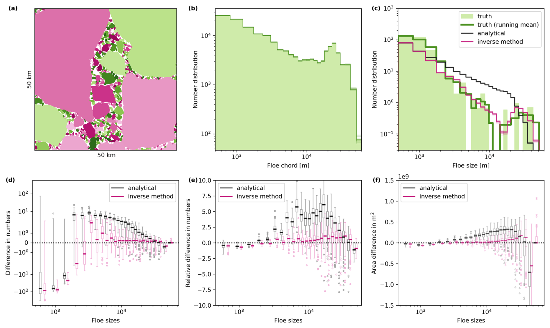
Figure 4 Evaluation of statistical method to convert FCD to FSD. Panel (a) shows one of the artificial floes masks generated to evaluate the conversion methods. Each floe is colored by a unique color. We randomly draw 30 000 lines over the mask in panel (a), measure floe chords along each, and create a FCD. This is repeated 25 times, and each distribution is plotted as a thin line in panel (b). The lines overlap over most of the chord bins, highlighting the convergence of the number density for this amount of lines. Panel (c) provides the known floe number size distribution for the floes in panel (a), along with the known distribution smoothened by a running mean with window size 3. All 25 floe size distributions determined from both the analytical solution and the inverse method for the mask in panel (a) are also shown in panel (c). The performance of both methods averaged over all 92 randomly drawn floe maps is given in the lower row. For each floe size bin the differences between both methods and the known size distribution is shown in box plots: (d) the difference in the number density, (e) the relative difference in the number density normalized by the known FSD, and (f) the difference in area covered by floes of each size.

We aim to evaluate the accuracy of our newly developed numerical method to convert FCDs into FSDs. To do so, we require realistic ice-ocean masks with known FSDs. As mentioned above, observational data of this kind did not already exist for wintertime pack-ice conditions. Therefore, we generate our own artificial ice-ocean masks with known FSDs by using the realistic floe shapes from the two observational datasets. To do so, we randomly draw, scale and place real floe shapes in a 50 by 50 km² box. Hereby, the floes are allowed to only partially lay within the box. Floes are also allowed to overlap with other floes by up to 5 pixels. This overlap mimics partially rafted floes which are frequently observed in consolidated winter ice conditions. One of the 92 generated masks is given in Fig. 4a, along with the measured FCD in Fig. 4b and the known FSD in Fig. 4c. We measure the FCD by again drawing 30 000 sampling lines over the generated floe masks and measure chord lengths along these lines. For each mask, we compute the FSD from the FCD using both our inverse method presented above and the analytical solution of Rothrock and Thorndike (1984) (for a full derivation, please refer to Appendix B). In Fig. 4c the results of both methods are compared against the known FSD. Both methods generally do not represent the spikiness of the known FSD and underestimate the amount of small floes present. To compare the general shape of the distribution we smooth the spikes of the true distribution with a running window of size 3. The distribution derived with the inverse method resembles the general shape of the distribution accurately. The distribution derived from the analytical solution shows a strong overestimation of medium-sized floes and an underestimation of very large floes, as expected given the different conditional probabilities (Fig. 3b). Statistics averaged over all 92 maps (Fig. 4d, e, f) generalize these results over a more diverse set of masks: Both methods strongly underestimate the amount of small floes (Fig. 4d), which can be explained by the allowed contact and overlap between floes. Contact between small floes results in “merged” medium-sized chords measured. Neither method can separate these “merged” chords, so both misattribute them to medium-sized floes, causing an overestimation in that size range. For medium to large floe sizes, the inverse method shows very good agreement, while the analytical solution overestimates the actual distribution by up to 5 times (Fig. 4e). Another problem of the analytical solution is strong overestimation of the area covered by ice in the mask by a factor of 2 (Fig. 4f). For the distribution computed with the inverse method, areal differences caused by uncertainties in the number distribution balance each other out such that the area covered by floes agrees well with the ice concentration of the mask. Backed by the results of this thorough evaluation, we choose to use the inverse method to determine FSDs from our measured FCDs.

3.3 Linking deformation to floe size evolution

The heart of our analysis is bringing together the drift derived deformation of ROIs and the observed changes in the FSD. This procedure is illustrated in Fig. 5. We define a 50×50 km² (1000 × 1000 pixels) large area of ice, our ROI, that we follow over two consecutive days (Fig. 5a). We advect the outline of the ROI in the first satellite image with the drift information to obtain the outline of the ROI in the second image (Fig. 5b). Using a line integral approximation along the boundaries of the ROI we compute the shear and divergence rates from the displacements of the boundary, which describes the deformation of the ROI (Lindsay and Stern, 2003). In parallel, we classify ice and open water in both images from the backscatter and deformation information (Fig. 5a, b) and measure the FCD of the ROI for both days (Fig. 5e). We compute the FSD for both days from the FCD with the inverse method presented above. Finally, we compute the change in FSD over both days and relate it to the deformation (Fig. 5f).

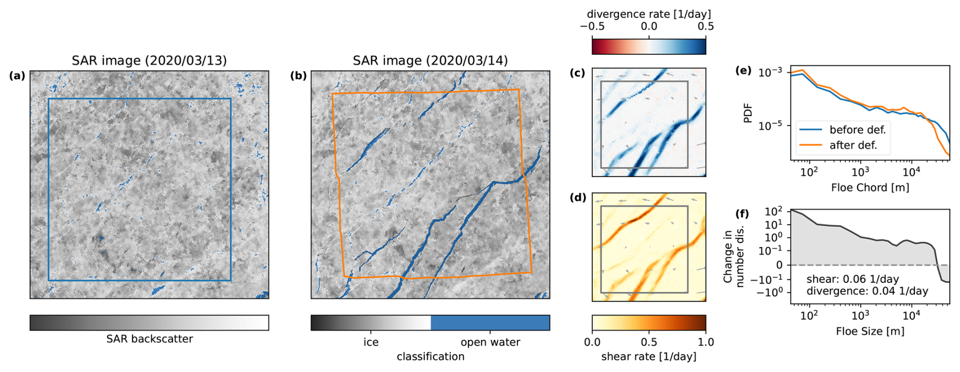
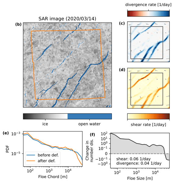
Figure 5 Linking the change in FCDs within a region of interest (ROI) to its deformation. (a) SAR image before the deformation event, (b) SAR image after deformation. Detected open water pixels are marked in blue in both SAR images. The ROI used to derive the deformation rate and the FCDs is indicated in blue in panel (a) and orange in panel (b). The deformation taking place in between the images is given in panel (c) for divergence and in panel (d) for shear. Panel (e) shows the FCDs before and after the deformation event. From the FCDs we compute FSDs and panel (f) shows the change in the number density of floe sizes during the deformation event, as well as the deformation rates of the ROI.

In our example highlighted in Fig. 5, we observe major fracturing of the ice cover between the two days with the opening of four lead systems (Fig. 5c, d). These openings are well captured by our open water classification, where the additional information from the backscatter signal allows us to clearly define the outline of the leads (Fig. 5b). As expected over the fracture event, we find that the number of long floe chords is reduced and shorter floe chords is increased. The transition between regimes is located around a floe chord of ∼ 20 km. Converting this trend into floe size, we find that during the fracture event the probabilities of floes larger than ∼ 30 km is reduced while smaller floes become more prevalent. We note here that this increase in number density gets more pronounced the smaller the floe size. In the following we will apply now the presented approach to entire data set to explore an general link between the deformation caused by fracture and the floe size distribution.

3.4 Evaluation of processing chain

The aim of this section is to test the robustness of our presented approach by evaluating the outcomes against independent observations where possible and perform physical consistency checks. As the uncertainties of the drift and deformation rates have been assessed in (Krumpen et al., 2021), we focus here on comparing the FCDs retrieved from SAR to independent estimates from ICESat-2 data and on testing how the opening recorded in the change in open-water mask relates to the divergence data derived from the drift product.

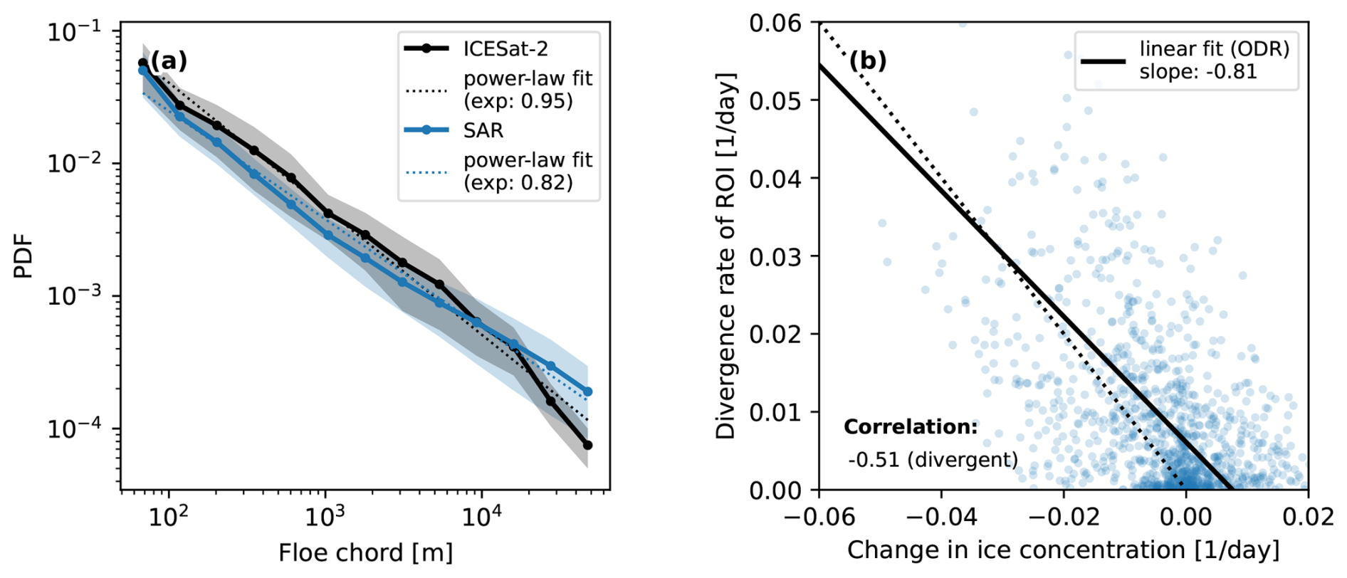
Figure 6 (a) Comparison of the FCD from the SAR-derived ice ocean mask with chords measured by the satellite altimeter ICESat-2 over all analyzed regions of interest. (b) Comparison of divergence rate of a ROI derived from SAR-based drift estimates with the change in ice concentration in the ROI as measured by the ice ocean mask for all ROI with divergent ice motion. A linear fit of both variables estimated with orthogonal distance regression (ODR) as well as their correlation are shown.

For the comparison of FCDs, we collect all available ICESat-2 data overlapping with the SAR images and use the SAR-derived drift information to correct for displacements caused by the different acquisitions times of Sentinel-1 and ICESat-2. Note that due to the 1 d temporal resolution of the drift data, this correction assumes homogeneous drift over 24 h and especially for strong drift regimes does not guarantee a reliable co-location at the pixel level. Therefore, we refrain from a pixel-based comparison of the SAR-derived open water mask with lead detections in ICESat-2 and focus on comparing the FCD for entire ROIs instead. For each ROI, where ICESat-2 data is available, we detect leads following a methodology akin to that of Petty et al. (2021). Floe chords are measured as the distance between leads, and we compute the FCD for the ROI. Next, we measure floe chords in the ROI based on the SAR ice-ocean mask using the method outlined above. Rarely, do we have more than one overpass from ICESat-2 over an ROI, while for SAR images we sample floe chords along 30 000 lines. To compensate for the effect of differing sample sizes on the chord distribution, we randomly subsample the floe chords measured in the SAR images to equal the number of samples from ICESat-2 for the ROI. To get an estimation of the uncertainty originating from the limited sample size, we repeat this random subsampling of SAR chords 50 times. Figure 6a shows that the distributions from the two satellites agree well within the error margins of one standard deviation, with the strongest differences for floes larger than 20 km. The under representation of large floes in ICESat-2 might stem from the far smaller sample size of ICESat-2 chords. Both distributions show a power-law behavior as previously reported (Stern et al., 2018b) with well aligned power-law exponents. Their strong agreement provides us with confidence that the presented workflow is well suited to measure floe chords from SAR images for wintertime sea ice.

In the second part of our method evaluation, we aim to quantify how well the change in ice concentration, which we determine from the ice-ocean masks, fits the divergence rate of the ROI. As we assume thermodynamic ice growth is negligible over 1 d, divergence should increase the open water and reduce ice concentration in the ice-ocean mask. In Fig. 6b both quantities are compared in a scatter plot. While we observe a low precision and wide spread between the variables, they are clearly anti correlated as assumed and show a reasonable linear relationship close to the one-to-one line. We attribute the wide spread mostly to the uncertainty in the SAR-derived open water mask and to a lesser extent to the data quality (and lower resolution) of the drift product. Part of this spread could also originate from more complex ROI deformations including rafting, compensating concurrent small-scale ridging, and fracturing or shear motion. This comparison shows that we can link these two SAR derived data sources of deformation and ice-ocean masks, especially as we will mainly analyze strongly divergent drift regimes ${\dot{\mathit{ϵ}}}_I>\mathrm{0.01}$ d⁻¹.

4 Results

We apply the processing chain presented above to all Sentinel-1 SAR images available during the period from March to May 2020 over the MOSAiC field site. In total, we analyzed 41 image pairs. In each image pair we define ROIs with a size of 50×50 km² that are half overlapping to obtain more data points while still not oversampling the data. These ROIs are tracked with the estimated drift between images, FSDs are measured in both images, and put in relation to the deformation taking place between scenes. Overall, we analyze 3352 ROIs and present their general ice conditions in Sect. 4.1 and their changes in floe size distribution as a function of deformation rates in Sect. 4.2. Finally, a parameterization of divergence triggered floe size redistribution is presented in Sect. 4.3.

4.1 General ice conditions

All ROIs in our analysis are located in consolidated pack ice with a mean ice concentration of 98 %. A summary of ice properties for all ROIs is provided in Fig. 7. We find that the ice concentration derived from our ice classification of SAR images agrees with AMSR2 ice concentration data (Beitsch et al., 2014, ftp://ftp.awi.de/sea_ice/product/amsr2, last access: 9 October 2026) well within the uncertainty range of 5 % for this dataset (Spreen et al., 2008; Krumpen et al., 2021) and both SAR derived and AMSR2 concentration have the same mean. We determine the ice freeboard of the ROIs from co-located ICESat-2 measurements. The median freeboard is 36 cm while the mean freeboard is 41 cm. The differences between median and mean freeboard in the ROIs indicates a heavy tailed freeboard distribution typical of pack ice shaped by deformation. In general, the ice conditions derived from our SAR-based ice classification and deformation computations are representative and agree well with other measurements for the region of the MOSAiC drift (Krumpen et al., 2021). For both ice concentration and freeboard we observe a slight reduction between the consecutive SAR images matching the mean divergent ice motion over all ROIs.

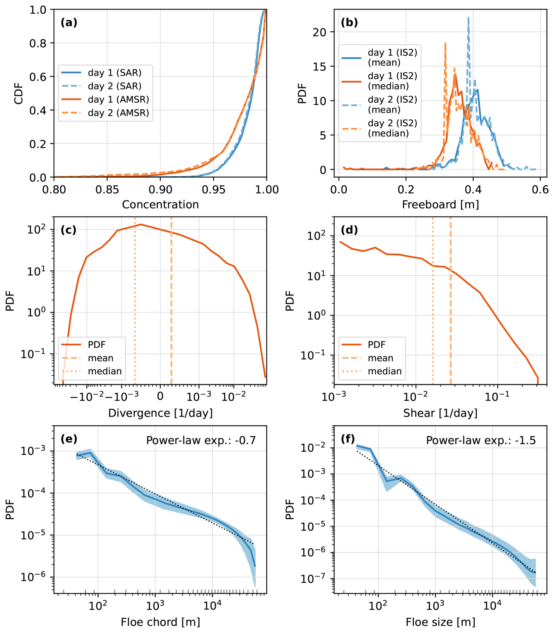
Figure 7 Overview of ice conditions in all regions of interest analyzed in this study. The cumulative probability distribution function (CDF) of the ice concentration for the ROI for both consecutive days is provided in panel (a). As a reference, we also present the ice concentration estimates derived from AMSR passive microwave instrument for the same ROIs. The distribution of the mean and median ice freeboard for all ROIs from ICESat-2 is shown in panel (b) again for both consecutive days. The PDF of the overall ROI divergence rates is shown in panel (c), highlighting a mean of $\mathrm{2.87}\times {\mathrm{10}}^{-\mathrm{4}}$ d⁻¹ and median of $-\mathrm{6.55}\times {\mathrm{10}}^{-\mathrm{4}}$ d⁻¹. Panel (d) shows the PDF of the overall ROI shear rates highlighting a mean shear rate of $\mathrm{2.67}\times {\mathrm{10}}^{-\mathrm{2}}$ d⁻¹ and median of $\mathrm{1.61}\times {\mathrm{10}}^{-\mathrm{2}}$ d⁻¹. The average floe chord distribution of all ROIs along with its standard deviation is shown (e) along with a power-law fit estimated by a linear fit in double logarithmic domain over the full floe chord and size range. Panel (f) provides the average floe size distribution of all ROIs with its standard deviation and power-law fit.

We find on average a divergent ice regime (Fig. 7c) as the mean divergence is positive, while the majority of ROIs are undergoing convergent ice motion (negative median divergence). This highlights the presence of strong divergence events related to fracturing and lead opening accompanied by periods and areas of weaker convergent ice drift that closes leads. The observed distribution of shear rates (Fig. 7d) shows a typical heavy tailed distribution.

The FCDs and FSDs averaged over all ROIs can be approximated by power-law distributions (Fig. 7e, f). For small chords and sizes (< 250 m) the distributions show effects of the discrete character of measured chords originating from the pixel resolution of the SAR images. For chord lengths approaching the size of ROI, deviations from the power-law distribution are caused by the finite size effect. Using simple linear fits to the double logarithmic data, we estimate exponents around 0.7 for the FCD and 1.5 for the FSD. We acknowledge that we do not properly test if the underlying distribution is described by a power-law (Clauset et al., 2009) – a discussion that is beyond the point of this side analysis – but presenting the exponents allows us to put our findings in context of other studies. Our power-law exponent of 1.5 for the FSD is at the lower end of the spectra but well within the distribution of power-law exponents found in literature (Stern et al., 2018b). A seasonal dependence of the FSD slope is well documented, with steeper exponents in fragmented summer conditions and shallower exponents in consolidated winter pack ice (Stern et al., 2018a). Our shallow exponent is therefore consistent with the winter conditions analyzed here, in contrast to the summer conditions studied in most previous studies.

4.2 Deformation related changes in the floe size distribution

The main focus of our study is to analyze the change in the FCD and FSD in relation to fracture by deformation. In Fig. 8 these changes are shown as differences in the number density of floe chords and sizes for all ROIs. In the following, we will also use the term chord or size redistribution referring to the change in the number density between consecutive days. We find a wide spread in the observed redistribution functions, which we attribute to the chaotic behavior of ice fracture. The exact number and positions of failure lines within a deforming ROI strongly depends on the presence of defects and existing failure lines in the ice cover, which is described by the distribution of floe sizes and their specific geometry and arrangement. On top of this chaotic spread driven by local ice conditions, general patterns emerge when grouping by the mode of deformation. When averaging over all strong divergent (${\dot{\mathit{ϵ}}}_I>\mathrm{0.01}$ d⁻¹) ROIs in our analysis, we measure a reduction in large floe chords (c≳20 km) and an increase in medium and small floe chords (c≲20 km). Converted into floe sizes, this equates to a decrease in floes of sizes larger than ∼ 33 km and an increase in floes smaller than ∼ 33 km, below we refer to the zero of the redistribution function as the unchanged floe parameter. Notably, the increase in small floes follows a power-law distribution, highlighting the importance of ice fracture in creating the power-law distribution of floe-sizes. These are the first direct observations showing power-law characteristics of fracture related redistribution of floe sizes. With this we provide observational grounding to the previous hypothesis that fracture processes are a driving factor in the power-law shape of the FSD (Weiss, 2003; Bateson et al., 2022). For convergent ice motion, we find significantly lower changes in the number density of floe chords. The observed redistribution becomes clearer when converted to floe sizes. The amount of large floes (d≳10 km) increases alongside a reduction of medium size floes (300 m ≲ d ≲ 10 km) following the general intuition that convergent ice motion facilitates coagulation of smaller floes to larger ones. This process also takes place at lower convergence rates, where in addition to medium size floes also small floes (d≲300 m) contribute to coagulation. The strong convergent states, which are averaged in Fig. 8, however, show an additional increase in small floes (d≲300 m), a clear sign of ice fracturing in compressive ice states accompanied by strong shear motion taking place simultaneously with a closing of the ice cover described above.

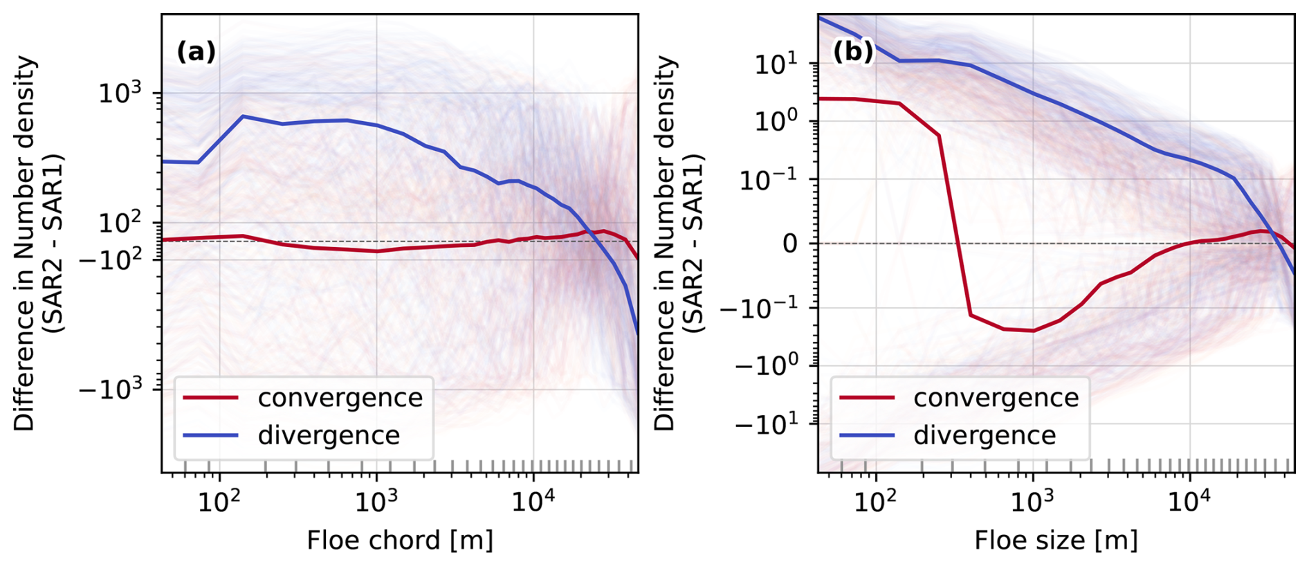
Figure 8 Overview of changes in the floe size distributions in all ROIs analyzed in this study: panel (a) shows the difference in floe chord number densities between two consecutive days. The shaded thin lines provides the observed change in number density for each individual ROI, color-coded by the divergence rate of the ROI. All clear divergent (${\dot{\mathit{ϵ}}}_I>\mathrm{0.01}$ d⁻¹) and convergent (${\dot{\mathit{ϵ}}}_I<-\mathrm{0.01}$ d⁻¹) ROIs are averaged and shown as thick blue and red lines respectively. (b) Same as panel (a) but for the change in floe size number density. The grey ticks along the x-axes denote the boundaries of the floe chord and size bins used to compute the number densities.

4.3 Development of a parameterization for fracture driven changes of floe size distribution

In the following section we will study the average floe size redistribution as a function of the deformation rate with the aim to derive a functional form that can be used as a parameterization in numerical models for the evolution of floe sizes. As discussed in the previous section, different initial FSD and ice conditions drive a chaotic non-linear behavior resulting in a large spread of the observed floe size redistributions. Given that a very large data sample would be required to describe these dependencies directly, we consider the floe size redistribution as a boundary value problem dependent only on the deformation of the ROI but independent of the initial ice conditions. Hence, we average redistribtions of multiple ROIs binned by similar divergence rates. Given the floe definition of the numerical model and the fact that we are only able to observe floes surrounded by open water in the satellite data, we limit this analysis to ROIs with divergent ice motion.

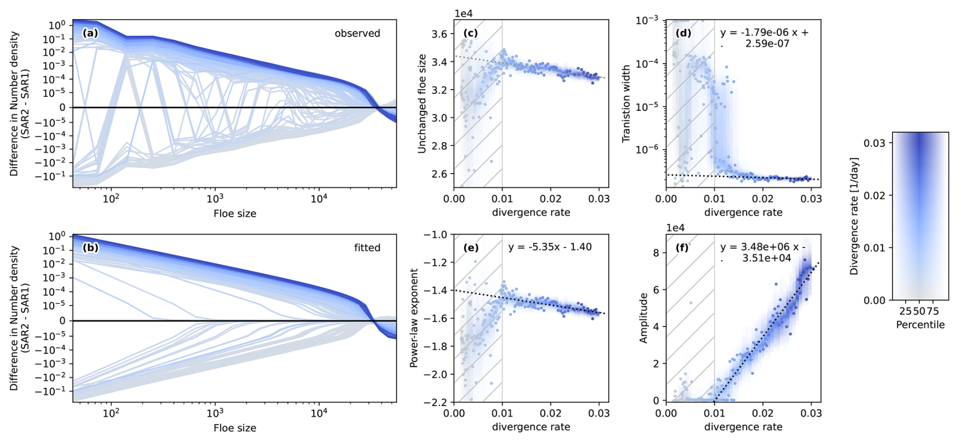
Figure 9 Difference in the number density of floe sizes between consecutive days as a function of divergence rates. Here, the number density is normalized by the width of the floe size bins used in the analysis. Therefore, we have to integrate the number density difference function over each floe size interval to obtain the number within the interval. In panel (a) we show these differences, where we average up to 100 ROIs binned by divergence rates (see detailed explanation in the text) for each line. We fit Eq. (10) to each of these averaged differences and show the fits in panel (b). The fitting parameters versus divergence rates are shown as follows: (c) unchanged floe size d₀, (d) transition width b, (e) power-law exponent e, and (f) the amplitude a. Here, the unchanged floe size (i.e., x-axis intercept of panel b) is not a free fitting parameter, but is determined from the other three fitting parameters by conserving the ice area during the deformation event. A linear fit that describes the dependence of the free fitting parameters on the divergence rate is provided as as a dashed black line in panels (d)–(f) along with the fitted slope and intersect. The linear fit is restricted to divergence rates ${\dot{\mathit{ϵ}}}_I>\mathrm{0.01}$ d⁻¹ excluding the hatched areas. To estimate the uncertainty of the fitted parameters of the change function, we repeat the drawing of ROIs for different divergence bins ten times. For each divergence bin the spread of fitted parameters is highlighted as a shaded contour plot in the background that shows the different percentiles of the distribution of fitted parameters. For clarity, we plot only one of the 10 subsamples in panels (a) and (b), for which the fitted parameters of the change function are highlighted as dots.

The divergence bins are defined by sorting the ROIs by divergence rate and eliminating ROIs with divergence rates ${\dot{\mathit{ϵ}}}_I<\mathrm{0.005}$ d⁻¹. Next, we create a bin centered at every second divergence value in our data ${\dot{\mathit{ϵ}}}_{I,c_i}$ and randomly draw up to 100 ROIs with similar divergence rates ($\left|{\log }_{\mathrm{10}}\right({\dot{\mathit{ϵ}}}_{I,c_i})-{\log }_{\mathrm{10}}({\dot{\mathit{ϵ}}}_{I,j}\left)\right|\le \mathrm{0.2}$). The floe size redistributions of all ROIs within each bin are averaged and shown as a function of divergence rate in Fig. 9a. If there are less than 100 ROIs within a certain divergence bin, all ROIs within the divergence bin get averaged. In the next step, we look for a functional form that describes the variation of these averaged redistributions as a function of divergence rate.

Based on the general form of redistribution for divergent ice motion discussed in the previous Sect. 4.2, we design a function that consists of the product of two major parts: (1) a power-law function describing the observed scaling for newly fractured floes and (2) a hyperbolic tangent that shifts the power-law from increasing the amount of small floes to decreasing the amount of large floes. The change in the floe size number density $\mathrm{\Delta }P\left(d,{\dot{\mathit{ϵ}}}_I\right)$ is therefore given by,

$$\begin{array}{}\text{(10)}& \mathrm{\Delta }P\left(d,{\dot{\mathit{ϵ}}}_I\right)=a\left({\dot{\mathit{ϵ}}}_I\right)d^{e\left({\dot{\mathit{ϵ}}}_I\right)}\tanh \left(b\left({\dot{\mathit{ϵ}}}_I\right)\left(d_{\mathrm{0}}\left({\dot{\mathit{ϵ}}}_I\right)-d\right)\right),\end{array}$$

where $a\left({\dot{\mathit{ϵ}}}_I\right)$ and $e\left({\dot{\mathit{ϵ}}}_I\right)$ are the amplitude and exponent of the power-law function respectively, $b\left({\dot{\mathit{ϵ}}}_I\right)$ is the transition width of the tangens hyperbolicus, and $d_{\mathrm{0}}\left({\dot{\mathit{ϵ}}}_I\right)$ is the intercept with the x-axis, which describes the unchanged floe size that is neither formed nor removed by the fracture event. All these parameters are assumed to be a function of the divergence rate.

We fit Eq. (10) to the average redistribution of each bin to determine its parameters. The functional form Eq. (10) has four parameters $a\left({\dot{\mathit{ϵ}}}_I\right)$, $e\left({\dot{\mathit{ϵ}}}_I\right)$, $b\left({\dot{\mathit{ϵ}}}_I\right)$, and $d_{\mathrm{0}}\left({\dot{\mathit{ϵ}}}_I\right)$, which need to determined by the fit. However, there is one additional constraint originating from the conservation of ice area, which reduces the amount of fitting parameters to three. As we only consider divergent ROIs, the ice cover only fractures and spreads out, while the overall area of ice within the ROI remains constant during the fracture event. Therefore the area gained by an increased amount of small floes need to be balanced by the ice area removed by decreasing the amount of large floes. This ice area conservation can be written as the following integral of the product of the observed FSD change with the floe area equating to zero,

$$\begin{array}{}\text{(11)}& \underset{\mathrm{0}}{\overset{\mathrm{\infty }}{\int }}\mathrm{\Delta }P\left(d,{\dot{\mathit{ϵ}}}_I|a,e,b,d_{\mathrm{0}}\right){\displaystyle \frac{\mathit{\pi }{d}^{\mathrm{2}}}{\mathrm{4}}}\mathrm{d}d\stackrel{\mathrm{!}}{=}\mathrm{0}.\end{array}$$

While we fit a, e, and b with a least squares fit, we use Eq. (11) to compute the unchanged floe size d₀ with the fitted parameters. Given the non-linearity of the integral, we cannot reformulate Eq. (11) into an analytical solution for d₀, but rather minimize the integral numerically within the fitting procedure. The fitted redistributions are given in Fig. 9b, showing good agreement with the observed redistributions. The fitted parameters as a function of divergence rate are provided in Fig. 9c, d, e, and f. To assess the uncertainty in the fitted parameters we repeat the random bin creation and fitting procedure 10 times. The resulting distribution of fitting parameters for each divergence rate bin is shown in Fig. 9c, d, e, and f. We find a large spread in the fitting parameter for small divergence rates ${\dot{\mathit{ϵ}}}_I<\mathrm{0.01}$ d⁻¹ hindering the derivation of a general form in this range. Multiple reasons could be responsible for this finding: (1) at these low divergence rate the initial conditions (FSD, concentration) are more important than the strength of the fracturing itself, and (2) the motion associated with low divergence rates could be realized with relative motion between existing floes without major fracturing occurring. For higher divergence rates ${\dot{\mathit{ϵ}}}_I>\mathrm{0.01}$ d⁻¹ we find a consistent evolution of all fitting parameters with increasing divergence rate indicating that fracturing of the ice cover is required to accommodate the ice motion in these strong divergence events, which leaves a distinct imprint on the observed redistributions. The dependence of the fitting parameters on the divergence rate can be approximated by linear functions,

$$\begin{array}{}\text{(12)}& {\displaystyle }a\left({\dot{\mathit{ϵ}}}_I\right)=a_{\mathrm{1}}{\dot{\mathit{ϵ}}}_I+a_{\mathrm{0}},\text{(13)}& {\displaystyle }e\left({\dot{\mathit{ϵ}}}_I\right)=e_{\mathrm{1}}{\dot{\mathit{ϵ}}}_I+e_{\mathrm{0}},\text{(14)}& {\displaystyle }b\left({\dot{\mathit{ϵ}}}_I\right)=b_{\mathrm{1}}{\dot{\mathit{ϵ}}}_I+b_{\mathrm{0}}.\end{array}$$

The amplitude a of the observed redistributions increases clearly with the divergence rate, while the power-law exponent e decreases with increasing divergence rate leading to a steepening of the power-law. The transition width b remains roughly constant with a slight decrease with increasing divergence rate. The unchanged floe size d₀ determined to fulfill Eq. (11) also decreases linearly with increasing divergence rate mainly driven by the decrease of the power-law exponent e. The slope and intercept of these linear relationships (Eq. 12–14) along with their uncertainty are summarized in Table 1.

Table 1 Parameters of the linear dependence of the fitting parameters on divergence rate following Eqs. (12)–(14).

4.4 Considerations for numerical implementation

In the process of implementing the parameterization given by Eq. (10) in a numerical model, a number of considerations are required to properly account for differences of spatial and temporal scales between the presented analysis and the model configuration used. First, the model could use a different choice of bins to discretize the floe size distribution. To account for this difference, the floe size redistributions (Fig. 9a and Eq. 10) are normalized by bin width. The integral of the floe size redistribution ΔP over a specific floe size range $d\in [d_i,d_{i+\mathrm{1}}]$ represents the change in the number density for that specific floe size bin. This change then is representative of the typical ROI size (50 km × 50 km = 2500 km²) and a time step of 1 d. For different horizontal grid cell areas and time steps in the model, the computed redistribution of the number FSD needs to be scaled accordingly. Besides the number FSD also the divergence rate is scale dependent, which also needs to be considered if grid cell area and time step do not align with the ROI values. Known power-law scaling relationships both in the temporal and spatial domain (Weiss, 2013; Hutter et al., 2018; Bouchat and Tremblay, 2020) can be used to adapt the divergence rate input in Eqs. (12)–(14) accordingly. The floe size redistribution function formulated for a model with a spatial resolution of Δx_m and a time step of Δt_m for a floe size bin $[d_{m,i},d_{m,i+\mathrm{1}}]$ is given by,

$$\begin{array}{}\text{(15)}& \begin{array}{rl}& \mathrm{\Delta }{P}_m\left(\left[d_{m,i},d_{m,i+\mathrm{1}}\right],{\dot{\mathit{ϵ}}}_{I,m}\right)={\left({\displaystyle \frac{\mathrm{\Delta }{x}_m}{\mathrm{50}\mathrm{km}}}\right)}^{\mathrm{2}}{\displaystyle \frac{\mathrm{\Delta }{t}_m}{\mathrm{1}\mathrm{d}}}\\ & \underset{d_{m,i}}{\overset{d_{m,i+\mathrm{1}}}{\int }}\mathrm{\Delta }P\left(d,{\left({\displaystyle \frac{\mathrm{50}\mathrm{km}}{\mathrm{\Delta }{x}_m}}\right)}^{-\mathit{\beta }}{\left({\displaystyle \frac{\mathrm{1}\mathrm{d}}{\mathrm{\Delta }{t}_m}}\right)}^{-\mathit{\alpha }}{\dot{\mathit{ϵ}}}_{I,m}\right)\mathrm{d}d,\end{array}\end{array}$$

where α and β are the temporal and spatial scaling exponent respectively (e.g. α=0.55 and β=0.49; Bouchat and Tremblay, 2020), and the subscript m marks model quantities. The scaled divergence rate within the integral should be used to compute the amplitude, exponent, and transition width. The unchanged floe size needs to be determined following the conservation of ice area Eq. (11). In this computation, it makes sense to account for floe size bins, where the computed redistribution exceeds the number of floes present in the bin.

5 Discussion and Conclusions

While we mainly study the effect of divergence-induced fracture on the floe size distribution in satellite data to develop a parameterization of this process for numerical models, we gained many additional scientific insights during the implementation of our data processing pipeline. We study the geometry of sea ice floes in great detail revealing scale invariant floe shapes over a range from several meters to a hundred kilometers. Scale invariance for floe sizes has been documented and discussed in detail in the literature (e.g. Rothrock and Thorndike, 1984; Stern et al., 2018b; Horvat and Tziperman, 2017), and proponents in this discussion have argued for a similarity across scales of the process forming and shaping floes. Our observation of scale independent floes geometries clearly supports this hypothesis. In addition, our analysis shows that the common assumption of circular shapes does not describe well the outline of floes characterized by small scale variation with sharp edges. Also, we find floes on average rather have a teardrop or egg shape, which could be used as an alternative if a general simplified shape of floes is required.

With our new knowledge about floe geometries, we extend the statistical considerations of the relationship between floe chord and size distributions from previous studies (Rothrock and Thorndike, 1984; Horvat et al., 2019) into an applicable conversion tool using an inverse numerical method. In doing so, only floe chords need to be measured over an ice-ocean mask, which does not require the sophisticated and delicate step of floe delineation and consequently saves computation time. Our method can be applied to satellite images from both winter and summer ice conditions, as well as 1 d altimetry data because only the ice-ocean mask is required. This opens the opportunity to derive full FSDs from CryoSat-2 and ICESat-2 in addition to the limited statistics presented in Horvat et al. (2019) and Petty et al. (2021) for model observation comparisons. We confirmed in a comprehensive evaluation using artificially generated floe maps that our method reliably estimates the floe size distribution while underestimating the amount of very small floes due to contacts between floes. Contact between floes, which are not resolve in the floe mask, complicate the statistical conversion as they alter the conditional probability $\stackrel{\mathrm{̃}}{G}(c/d)$ in direct dependence on the FSD, which we currently neglect. Using an iterative process between solving for the FSD P and modifying the conditional probabilities $\stackrel{\mathrm{̃}}{\mathbf{F}}$, this dependency could be incorporated in the conversion tool in future work.

The backbone of our study is the combination of SAR-based deformation and drift data with image based ice classification providing concurrent information about floe size changes and occurring deformation and fracture. Compared to newly AI-based methods under development that distinguish multiple ice types (e.g. Guo et al., 2022; Kortum et al., 2024), we use a rather simplified image classification method to only distinguish ice and open water. For our application of generating ice-ocean masks to measure floe chords, the method is adequate, as the agreement with concurrent chord estimates from ICESat-2 shows. In some instances we observed our classification scheme to falsely classify pressure ridges as leads (not shown), which could be addressed by more sophisticated classification algorithms in the future to specifically target also the classification of deformed ice. New machine learning methods could also be applied in the drift estimation from consecutive SAR images, as Uusinoka et al. (2025) successfully shown for ship-borne radar images. These methods allow for drift estimates up to pixel resolution potentially enabling fully dynamic based definitions of floe boundaries. Especially in consolidated winter ice conditions the combination of open water classification and detection of regions with discontinuous ice motion would offer a clear identification of floe boundaries. In future work, higher resolution input data both from different satellite platforms, like Terra SAR-X (Hwang et al., 2017; Kortum et al., 2024), or from ship-based radar (Uusinoka et al., 2025), would allow one to explore a potential scale-break for the power-law shaped redistributions at meter scale. Ultimately, ensemble simulations of discrete element models (DEMs) for sea ice would be the ideal tool to map floe redistributions for different FSD and deformation scenarios, once their formulation of contact forces and large-scale fracture are found to be realistic in a comparison against observational data (Åström et al., 2024).

In our analysis we find clear floe redistribution for both divergent and convergent deformation events, where for strong deformation $\left|{\dot{\mathit{ϵ}}}_{\mathrm{I}}\right|>\mathrm{0.01}$ d⁻¹ imprints of fracturing are clearly visible with an increase of small floes. Also, we find that both divergent and convergent events are associated with shear rates exceeding in magnitude the divergence rates. This suggest in line with previous literature (Ringeisen et al., 2023) that the material fails in shear, fractures, and either opens up the ice cover or collides and piles up. While in convergence the ice cover closes up by merging medium size floes to ice conglomerates seen as large floes, fracturing along compressive faults and ridges manifests in an increase in small floes. However, the observed redistributions for convergent ice motion are more diverse, which partly could be explained by fact that our processing chain does not fully resolve boundaries of floes between floes in full contact with each other. Therefore, we refrain from studying convergent floe redistribution in detail and suggest to use DEM simulations for this purpose in the future.

For fracture in divergent ice motion, we find that the observed floe size redistributions are well described by a functional form that depends on the divergent rate. This functional form describes a reduction of large floes and an increase in small floes following a power-law dependence on the floe size. With this, we present the first observational process study backing previous hypothesis that the internal fracture is the main driver of power-law distribution of floe sizes (Weiss, 2003; Bateson et al., 2022). The parameters of our suggested fitting function change linearly with divergent rates and we determine this change based with the observed redistribution. With increasing divergence rates more large floes are broken into an increasing number of small floes, while the unchanged floe size remains stable over a range of divergence rates. We note here that the amount of floe area redistributed by the fitted function saturates for divergence rates higher 0.03 d⁻¹, as the increase of the amplitude is balanced by the steepening of the power-law. A saturation of the redistributed floe area is plausible given that once the ice cover is heavily fractured no additional fracture of floes is necessary to accommodate additional divergent motion. In that case, stronger divergence rates just lead to an increase in open water and not the amount of fracture. However, analysis of far more satellite images would be required to sample the few scenes with divergence rates exceeding 0.03 d⁻¹ to test this hypothesis. Using the parameters provided in Table 1 the suggested parameterization will lead to a decreasing amount of redistributed floe area for large divergence rates ${\dot{\mathit{ϵ}}}_I>\mathrm{0.03}$ d⁻¹, which is not desired. Therefore, we suggest to use this value as an upper threshold to fix the redistribution for all higher divergence rates when implementing the scheme in a numerical model.

To implement our suggested parameterization for fracture driven floe size redistribution, we present a general form that accounts for the bins used to describe the modeled floe size distribution, as well as different spatial and temporal resolution. This formulation allows one to relate the modeled ice conditions with the characteristics found in our observational study. However, even state-of-the-art sea ice models do not fully capture the magnitude, spatio-temporal localization and characteristics of observed sea ice deformation fully (Bouchat et al., 2022; Hutter et al., 2022). In this light, the functional form found in this study defines the shape of the redistribution function versus divergence rate, while individual parameters can and should be optimized within the numerical model by comparing simulated FSDs with observations to account for model specific ice dynamics.

Once implemented the new fracture redistribution scheme will complement the FSD formulation within the sea ice model CICE and will allow to simulate all relevant processes shaping the FSD not only in the marginal ice zone but also in consolidated pack ice. In this framework complex interactions between dynamic and thermodynamic processes in the ice, such as the effect major fracturing occurring in Arctic cyclones on consequent lateral melt or reduced wave attenuation, could be studied as well as their implications on the interaction with the atmosphere and ocean. With our fracture induced redistribution scheme, the simulated FSD also holds memory of past deformation and is therefore a measure for ice integrity. This opens the potential to model the complex two-way feedback between deformation and FSD, where ice strength is modulated depending on the FSD allowing for brittle behavior in standard dynamical models.

Appendix A: Spatial data coverage

The spatial location of all SAR scences analyzed in this study is shown in Fig. A1.

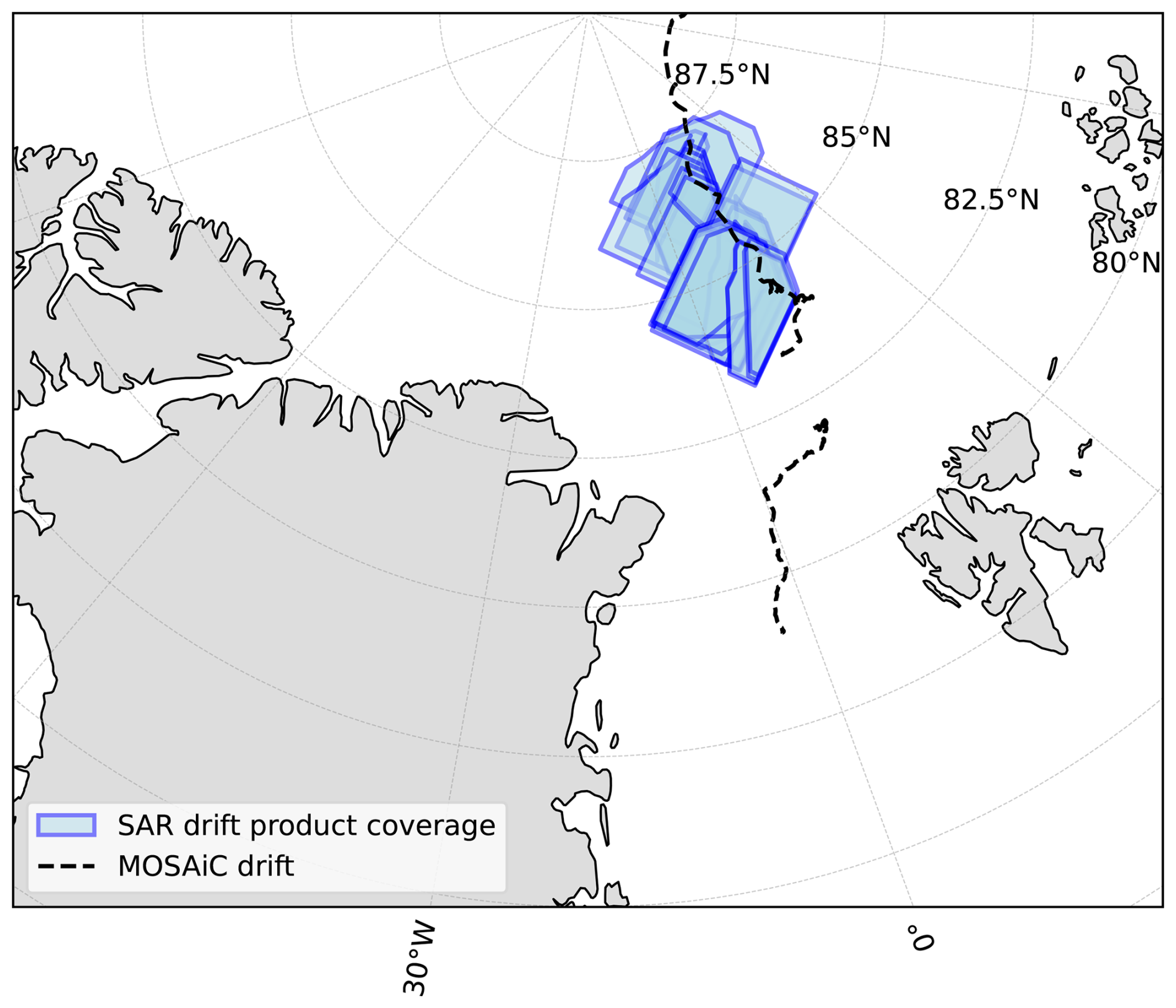
Figure A1 Overview of the spatial location of all SAR scenes analyzed in this study. Sentinel SAR images were cropped to 400×400 km² area centered around Polarstern, following the spatial coverage of the SAR drift product (von Albedyll and Hutter, 2023) used in this study. The dashed line shows the passive drift track during MOSAiC. In this study we only use SAR images between 13 March and 31 May 2020.

Appendix B: Derivation of analytical statistical conversion for circular floes

This appendix presents the full derivation of the analytical solution to the statistical conversion between FCD and FSD assuming circular floes as used in the paper. This derivation uses the same variables definition presented in Sect. 3.2.2 and begins with the Bayes' theorem linking FCD and FSD,

$$\begin{array}{}\text{(B1)}& F(d;c)S\left(c\right)=\stackrel{\mathrm{̃}}{F}(c;d)P\left(d\right),\end{array}$$

where S(c) is the floe chord distribution and P(d) the floe size distribution. F(d;c) is the conditional probability where F(d;c)dd describes the probability that floes of size d to d+dd were sampled given that we measure the floe chord c. Respectively, $\stackrel{\mathrm{̃}}{F}(c;d)\mathrm{d}c$ is the conditional probability to measure floe chords of c to c+dc given that a floe of size d is sampled. While F(d,c) is unknown, we can determine $\stackrel{\mathrm{̃}}{F}(c;d)$ by regarding it as a combination of a geometrical problem and sampling probability,

$$\begin{array}{}\text{(B2)}& \stackrel{\mathrm{̃}}{F}(c;d)=G(c;d)H\left(d\right),\end{array}$$

where H(d) is the probability that a floe of size d is sampled by a randomly drawn line, and G(c;d) describes the probability of to measure floe chord c given that the randomly drawn line hits a floe of size r (Rothrock and Thorndike, 1984). The further derivation assumes circular floes. A chord sampling line can hit a floe at an intersection angle $\mathit{\gamma }\in [\mathrm{0},\frac{\mathit{\pi }}{\mathrm{2}})$, where γ is defined as the angle between the sampling line and the tangent to floe boundary at the point, where the sampling line hits the floe. In the following, we will follow formulation of the interior angle θ that Horvat et al. (2019) introduced in Fig. 1 of their paper, which relates to the intersection angle by θ=2γ. Using the interior angle, the following relationship between chord length and floe size is given by,

$$\begin{array}{}\text{(B3)}& c=d\sin \left({\displaystyle \frac{\mathit{\theta }}{\mathrm{2}}}\right)\iff \mathit{\theta }=\mathrm{2}\arcsin \left({\displaystyle \frac{c}{d}}\right),\end{array}$$

where we use again the diameter of a circular floe as the floe size d. Assuming all intersection angles are equally likely,

$$\begin{array}{}\text{(B4)}& T\left(\mathit{\theta };d\right)={\displaystyle \frac{\mathrm{1}}{\mathit{\pi }}}\mathrm{for}\mathit{\theta }\in \left]\mathrm{0},\mathit{\pi }\right],\end{array}$$

where T(θ;d) is the conditional probability to hit a floe at an angle θ given the size d, we can derive an analytical description of the conditional probability G(c;d),

$$\begin{array}{}\text{(B5)}& {\displaystyle }\underset{\mathrm{0}}{\overset{\mathrm{\infty }}{\int }}G(c;d)\mathrm{d}c=\underset{\mathrm{0}}{\overset{\mathit{\pi }}{\int }}T\left(\mathit{\theta };d\right){\displaystyle \frac{\mathrm{d}\mathit{\theta }}{\mathrm{d}c}}\mathrm{d}c,\text{(B6)}& {\displaystyle \frac{\mathrm{d}\mathit{\theta }}{\mathrm{d}c}}={\displaystyle \frac{\mathrm{d}}{\mathrm{d}c}}\left(\mathrm{2}\arcsin \left({\displaystyle \frac{c}{d}}\right)\right)={\displaystyle \frac{\mathrm{2}}{\sqrt{d^{\mathrm{2}}-c^{\mathrm{2}}}}},\end{array}$$

$$\begin{array}{}\text{(B7)}& G(c;d)={\displaystyle \frac{\mathrm{2}}{\mathit{\pi }}}{\displaystyle \frac{\mathrm{1}}{\sqrt{d^{\mathrm{2}}-c^{\mathrm{2}}}}}.\end{array}$$

The sampling probability H(d) is simply given by the floe size d in our 2D sampling approach,

$$\begin{array}{}\text{(B8)}& H\left(d\right)=d.\end{array}$$

By definition the integral of the conditional probability F(d;c) over floe size d equals one, such that we obtain,

$$\begin{array}{}\text{(B9)}& {\displaystyle }S\left(c\right)& {\displaystyle }=\underset{\mathrm{0}}{\overset{\mathrm{\infty }}{\int }}\stackrel{\mathrm{̃}}{F}(c;d)P\left(d\right)\mathrm{d}d,\text{(B10)}& {\displaystyle }& {\displaystyle }=\underset{\mathrm{0}}{\overset{\mathrm{\infty }}{\int }}{\displaystyle \frac{\mathrm{2}}{\mathit{\pi }}}{\displaystyle \frac{d}{\sqrt{d^{\mathrm{2}}-c^{\mathrm{2}}}}}P\left(d\right)\mathrm{d}d,\end{array}$$

by integrate Eq. (5) over the floe size d.

This integral in Eq. (B9) is a form of the general formulation of the Abel transform,

$$\begin{array}{}\text{(B11)}& \begin{array}{rl}& F\left(y\right)=\mathrm{2}\underset{y}{\overset{\mathrm{\infty }}{\int }}{\displaystyle \frac{f\left(r\right)r}{\sqrt{r^{\mathrm{2}}-y^{\mathrm{2}}}}}\mathrm{d}r\Rightarrow \\ & f\left(r\right)=-{\displaystyle \frac{\mathrm{1}}{\mathit{\pi }}}\underset{r}{\overset{\mathrm{\infty }}{\int }}{\displaystyle \frac{\mathrm{d}F}{\mathrm{d}y}}{\displaystyle \frac{\mathrm{d}y}{\sqrt{y^{\mathrm{2}}-r^{\mathrm{2}}}}}.\end{array}\end{array}$$

Using Eq. (B11) to transform the integral formulation of the FCD in Eq. (B9), we obtain an integral formulation of the FSD,

$$\begin{array}{}\text{(B12)}& P\left(d\right)=-\underset{R}{\overset{\mathrm{\infty }}{\int }}{\displaystyle \frac{\mathrm{d}S\left(c\right)}{\mathrm{d}c}}{\displaystyle \frac{\mathrm{1}}{\sqrt{c^{\mathrm{2}}-d^{\mathrm{2}}}}}\mathrm{d}c,\end{array}$$

which allows to compute the FSD from FCD analytically assuming circular floes. This formulation has been used to compute the reference FSDs in Sect. 3.2.4.