Transition to a much warmer climate for the global ocean and Antarctic Ice Sheet coupled system, and its reversibility

In Antarctica, two plausible tipping points have been suggested: an ocean tipping point involving a cold-to-warm transition of ice-shelf cavities, and an ice-sheet tipping point associated with the marine ice-sheet instability. This study explores the existence of such tipping points at the scale of Antarctica, using a coupled ocean–ice-sheet model. We first apply and then remove an abrupt perturbation to the ocean, instantaneously switching the atmospheric forcing to high-end 23rd century conditions, which shifts all ice-shelf cavities of Antarctica to warm conditions. With the assumption of fixed ice-shelf front positions, our simulations reveal that Antarctic continental shelf waters rapidly warm, leading to a regime shift with increased ice-shelf melt rates, significant ice-shelf thinning, and retreat of ice-sheet grounding lines. The ocean conditions reverse within 40 years when the atmospheric perturbation ceases, while the ice sheet’s response is much slower. Some regions of East Antarctica show signs of ice-sheet reversibility over several centuries. In contrast, we identify 14 ice streams, primarily in the Ross, Amundsen, Filchner, Ronne, and Dronning Maud Land basins, that still undergo irreversible retreat several centuries after the removal of the perturbation.

1 Introduction

Tipping points occur when changes in large parts of the climate system, known as tipping elements, become self-perpetuating beyond a forcing threshold (McKay et al., 2022). This involves the presence of feedbacks that amplify the response to a forcing perturbation. In this case, the system often reorganises into a state that remains stable when the perturbation is removed. As a result, plotting a state variable versus the forcing variable appears as a hysteresis with possible bistable steady states in a range of forcing values. Transitions in and out of this range can thus appear irreversible.

In Antarctica, two plausible tipping points have been suggested: (i) an ocean tipping point in which an ice-shelf cavity switches from a cold state with low melt rates to a warm state with high melt rates (Hellmer et al., 2017), and (ii) an ice-sheet tipping point, often described in terms of ice-sheet instability (Weertman, 1974), in which the grounded ice flow abruptly accelerates, thinning the ice sheet and ice shelves, while the grounding line retreats inland.

The cold and warm ocean states mentioned above are associated with different melt regimes, as identified by Jacobs et al. (1992): melting by high-salinity shelf water formed during winter freezing (Mode 1) and melting by warm Circumpolar Deep Water intrusions (Mode 2). Jacobs et al. (1992) also identified a third mode of melting in shallow areas, driven by tidal pumping and seasonal warming of coastal currents. Hellmer et al. (2017) found that the cold-to-warm ocean transition of the Filchner-Ronne cavity under future scenarios was irreversible in the sense that basal melting of the ice shelf had to be artificially suppressed to return to the original state once the atmospheric perturbation was removed. Hazel and Stewart (2020) also reported a bi-stability of the thermal state of this cavity, depending on the history of idealised wind forcing perturbations. In contrast, Haid et al. (2023) and Reese et al. (2026) gave a more contrasted picture: their reversed atmospheric perturbation experiments indicated reversibility of the Filchner-Ronne cavity, although the ocean required several decades to return to its initial state. Haid et al. (2023) nonetheless identified some sensitivity to the initial state across a range of atmospheric forcing, which suggested some bi-stability. Additionally, Caillet et al. (2023) suggested that similar cold-to-warm ocean transitions may have occurred in the Amundsen Sea after the pre-industrial era, but reversed perturbation experiments showed reversibility within a few decades in this case. Given the computational cost of the ocean models used in these studies and the large number of degrees of freedom of the atmospheric forcing, systematic experiments with slowly varying perturbations and multiple reversals, as performed in ice-sheet modelling studies (e.g., Garbe et al., 2020; Rosier et al., 2021), remain computationally challenging for ocean models. Consequently, a systematic analysis of hysteresis and reversibility for the ocean remains lacking, including in the present study.

The ice-sheet tipping behaviour in Antarctica is often discussed in the context of the so-called marine ice-sheet instability (MISI). As discussed by Sergienko et al. (2026), this term is used in the literature to describe several related but distinct concepts, some of them purely related to the ice and bedrock configuration (e.g. Weertman, 1974; Schoof, 2007; Gudmundsson et al., 2012), and others involving the forcing by ice-shelf melting and the consequences on ice-shelf thinning, reduced buttressing, and grounding-line retreat (e.g. Hill et al., 2023; Reese et al., 2023). In this article, we use “instability” to refer to a forced ice-sheet response that becomes self-sustained (for any reason) for at least several centuries.

While the recent retreat of Antarctic grounding lines may not yet be irreversible or self-sustained (Hill et al., 2023), there is observational evidence of recent ocean and sea-ice regime shifts in Antarctica (Abram et al., 2025). Further grounding-line retreat could eventually lead to the irreversible collapse of some marine regions of West Antarctica even under present-day climate conditions (Reese et al., 2023). A complete collapse of the West Antarctic Ice Sheet may be committed if global warming reaches 2 °C above pre-industrial conditions (Garbe et al., 2020) or if the Amundsen Sea warms by more than 1.2 °C above present-day conditions (Rosier et al., 2021) or even less (Chandler et al., 2025). However, confidence in the parameterised ice-shelf melt rates under future conditions remains low (Burgard et al., 2022, 2023) and not representing the ocean feedbacks is equivalent to assuming that there is an unbounded amount of heat available for ice-shelf melting, which is wrong (Sergienko et al., 2026).

This study investigates, in a consistent global ocean framework, the reversibility of the ocean cold-to-warm transition in 25 major ice-shelf cavities of Antarctica, as well as the potential for cascading effects, specifically, whether ocean–ice-sheet feedbacks promote irreversibility of ocean and ice-sheet changes. To address these questions, we use a global coupled ocean–ice-sheet model at a relatively high resolution, here 0.25°. As described in Mathiot and Jourdain (2023, hereafter MJ2023), strong perturbations of the atmosphere are required to trigger a cold-to-warm transition across all Antarctic ice shelves. In this study, we therefore focus on the reversibility of the ocean–ice-sheet response to the large-scale perturbation used in MJ2023, rather than systematically mapping hysteresis or identifying transition thresholds.

2 Ocean–sea-ice–ice-shelf simulations

2.1 Coupled ocean–sea-ice–ice-sheet Model

The ocean–ice-sheet model used in this study consists of a coupling between the NEMO global ocean component and the Elmer/Ice Antarctic ice-sheet component. These two components were previously coupled in a very simple configuration representing a single ice shelf (Favier et al., 2019), but the coupling framework has been completely revised since then. The two individual components and the coupling interface are described hereafter. Some experiments make use of the standalone Elmer/Ice model (i.e., uncoupled to NEMO), with the same model set-up, except for ice-shelf basal melting, which is prescribed in the standalone version.

2.1.1 Ocean–sea-ice component: NEMO

We use version 4.0.4 of the three-dimensional primitive-equation ocean–sea-ice model NEMO (Nucleus for European Modelling of the Ocean; Madec et al., 2019). The model is configured on a global grid with a nominal horizontal resolution of 0.25° (approximately 8 km at 70° S), which is sufficient to represent the main features of ocean circulation beneath Antarctic ice shelves (Mathiot et al., 2017). A comprehensive description and evaluation of this configuration are provided in MJ2023; here, only the key elements are outlined. The vertical discretisation relies on a z^* coordinate system (Adcroft and Campin, 2004), using 121 levels with variable spacing: resolution is about 1 m near the surface, around 20 m between 100 and 1000 m depth, and becomes coarser in deeper layers. Sea-ice processes are simulated with the SI3 model (Rousset et al., 2015), while icebergs are represented as Lagrangian particles (Marsh et al., 2015; Merino et al., 2016). Basal melting beneath ice shelves is computed using the three-equation formulation (Holland and Jenkins, 1999; Asay-Davis et al., 2016). In this framework, the effect of tides is included via a spatially varying background velocity derived from the CATS2008 model (Padman et al., 2008), following the approach of Jourdain et al. (2019). The bathymetry of the Antarctic continental shelf, as well as the ice-shelf draft, are prescribed from BedMachine Antarctica version 2 (Morlighem et al., 2020; Morlighem, 2020).

2.1.2 Ice-sheet component: Elmer/Ice

We use the Elmer/Ice model to simulate the evolution of the ice sheet (Gagliardini et al., 2013). The configuration employed here is briefly described below, while a comprehensive presentation is available in Hill et al. (2023). Ice flow is computed by solving the Shallow Shelf Approximation (SSA) to the Stokes equations, assuming an isotropic rheology described by Glen’s flow law. The initial ice-sheet geometry is prescribed from BedMachine Antarctica version 2 (Morlighem et al., 2020; Morlighem, 2020). Ice viscosity and basal friction are inferred by inversion using ice thickness observations primarily from 2009–2019 (Morlighem et al., 2020; Morlighem, 2020) together with surface ice velocity data from a 2015–2016 snapshot provided by the MEaSUREs Annual Ice Velocity Maps dataset (Mouginot et al., 2019). The viscosity and friction parameters are kept constant in time. In floating regions, where inversion is not applicable, basal friction is set to a constant value of 1 Pa m⁻¹ a, consistent with a linear Weertman sliding law (Weertman, 1974).

Boundary conditions assume fixed ice shelf front positions, and no basal melting is applied beneath grounded ice or partially floating grid cells. The surface mass balance is derived from the climatology of the atmosphere–snow model of van Wessem et al. (2018) and is held constant throughout the simulations, as the focus is on ocean–ice-sheet tipping processes. The representation of basal mass balance is described in Sect. 2.1.3. The grounding-line position is determined using a flotation criterion, and basal friction in partially floating elements is treated using a sub-grid parameterisation (SEP3; Seroussi et al., 2014). The computational mesh is anisotropic, with a horizontal resolution ranging from 1 km near the grounding line to 50 km in the interior, and remains fixed during the simulations. Such a resolution in the grounding-line area, combined with sub-element parameterisation, is known to be sufficient to accurately represent grounding-line migrations (Seroussi et al., 2014). Furthermore, this resolution also allows accurate representation of small pinning points, which are critical for ice-sheet stability (Favier et al., 2016).

Prior to the prognostic simulations, a relaxation phase is performed to limit inconsistencies between the initial input fields and the inverted state when transitioning from diagnostic to prognostic simulation (Gillet-Chaulet et al., 2012). The model is first integrated for 5 years using the linear Weertman sliding law (Weertman, 1974), consistent with the inversion procedure used to derive basal friction coefficients. This initial phase is followed by an additional 15 years of relaxation employing a regularised Coulomb friction law (Joughin et al., 2019). The corresponding parameters are obtained from the previously inverted linear friction coefficients, following Brondex et al. (2019).

2.1.3 The ocean–ice-sheet coupling interface

In the coupled configuration, exchanges between NEMO and Elmer/Ice are performed annually. Ocean-induced basal melt rates computed by NEMO are provided to Elmer/Ice, while Elmer/Ice supplies NEMO with updated ice-shelf basal topography and the ice flux lost at the ice-shelf front. Given the fixed ice-shelf front position in the present configuration, this flux corresponds directly to the ice flux computed at the front and is hereafter referred to as the iceberg calving flux. The two models are run sequentially over each coupling interval: NEMO first simulates ocean dynamics over one year and provides the corresponding annual mean basal mass balance beneath ice shelves, after which Elmer/Ice simulates ice-sheet evolution over the same period and returns the updated ice-shelf geometry along with yearly averaged iceberg calving fluxes. Within this framework, no temporal lag is introduced for basal melt rates between the two models. In contrast, the ice-shelf topography used by NEMO progressively lags behind that simulated by Elmer/Ice, ranging from no delay at the beginning of the year to approximately one year at its end. Additionally, iceberg calving fluxes used in NEMO’s Lagrangian iceberg model are delayed by one year relative to the ice dynamics simulated by Elmer/Ice. This coupling strategy is broadly consistent with previous approaches described by Smith et al. (2021) and Pelletier et al. (2022).

The interpolation of Elmer/Ice topography to each NEMO grid point is made using the natural finite element interpolation from Elmer/Ice. Iceberg calving fluxes are transposed onto the NEMO grid by routing, for each coastal Elmer/Ice element, the iceberg calving flux toward the nearest NEMO ocean cell. The interpolation of the NEMO melt rate onto the Elmer grid is first obtained through a conservative interpolation. Then, because of inconsistencies between the grounding lines of NEMO and Elmer/Ice, any ice-shelf mesh of Elmer/Ice with no corresponding ice shelf mesh in NEMO is filled with melt rates from the nearest ice shelf cells. Conversely, if the conservative interpolation gives a non-zero melt rate beneath a grounded mesh in Elmer/Ice, it is set to zero.

In the absence of an evolving ice front and for the sake of numerical stability of the ice-sheet model, we keep imposing a minimum ice shelf thickness of 1 m in the coupled system. Beneath such 1 m thick ice, basal melt rates are still simulated in NEMO, and the 1 m cap imposed in Elmer/Ice is equivalent to a spurious mass flux injected in the coupled system, i.e. there is no mass conservation. The importance of melting in these areas, hereafter referred to as “pseudo-collapsed areas”, is presented with our results.

2.2 Experiments

To build the initial state of the coupled model, we start from a first guess consisting of the ice-sheet geometry after the 20-year relaxation described in Sect. 2.1.2 and the ocean state from the year 1999 of MJ2023's reference (after 20 years of spin-up). This produces inconsistent initial conditions between Elmer/Ice and NEMO because the ocean state and geometry of the under-ice shelf cavities provided by the Elmer/Ice initialisation differ from those in the standalone versions. To reduce this inconsistency, which can be locally large, the first-guess ocean state is extrapolated to fit the Elmer/Ice topography at the end of the relaxation, and NEMO is run for 5 more years with this steady topography. Then Elmer/Ice is run for an additional 5 years beyond the first guess, with the basal melt computed by NEMO in its 5th year. A schematic of the initialisation procedure is available in Fig. 1.

The additional 5-year ocean relaxation is sufficient to flush most of the cavities and bring basal melt rates into equilibrium with the updated ice geometry. The subsequent 5-year ice-sheet relaxation allows the ice sheet to adjust rapidly to the changes in basal melt, while slower adjustments occur over the first decades of the simulation. Since this study primarily compares results with a reference simulation, these longer-term, slow adjustments do not affect our conclusions.

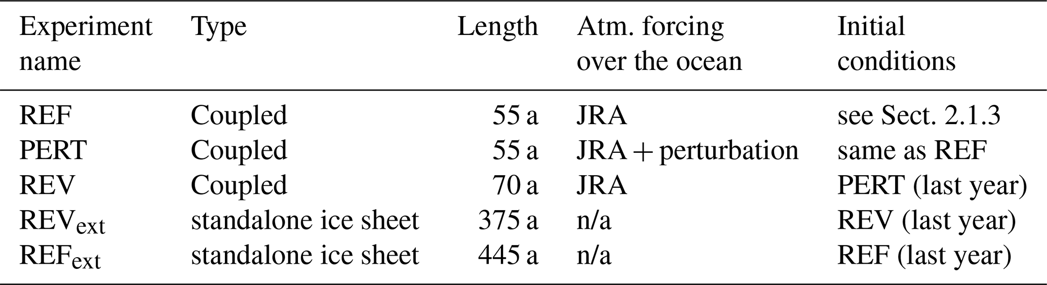
This initialized state is subsequently used for three main experiments: the reference simulation (REF), a perturbed scenario (PERT), and a reversibility run (REV), as described below and in Table 1.

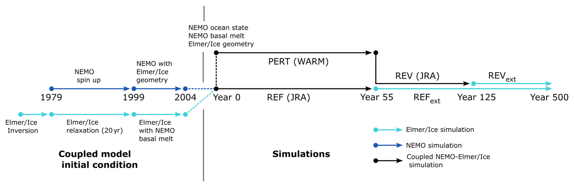
Figure 1 Illustration of the coupled model initialization procedure (left) and the simulation protocol (right).

In all experiments, the ice-sheet surface mass balance is prescribed from the climatology of van Wessem et al. (2018) and is held constant in time, so that the simulated ice-sheet evolution reflects only ocean–ice-sheet interactions.

In terms of atmospheric forcing over the ocean, our strategy is almost identical to that of MJ2023. The reference experiment (REF) is a present-day simulation driven by the JRA55-do version 1.4 atmospheric reanalysis (Tsujino et al., 2018), which provides 3-hourly atmospheric fields at 55 km resolution and captures realistic interannual variability over the period 1858–2018. In this study, we restrict the JRA period to the satellite era (1979–2018). The perturbed experiment (PERT) is an idealised abrupt shift to high-end atmospheric conditions representative of the end of the 23rd century. PERT starts from the same initial state as REF. We also run a reversibility experiment (REV), which begins from the last year of PERT and is subsequently driven by the same atmospheric forcing as REF.

The atmospheric forcing applied in PERT follows MJ2023. It retains both the mean state and interannual variability of JRA55-do, onto which monthly anomalies are superimposed for all variables used in the computation of ocean surface boundary conditions. These anomalies are defined as the difference between 2260–2299 and 1975–2014 and are derived from monthly outputs of the IPSL-CM6A-LR climate model (Boucher et al., 2020) under the SSP5-8.5 emission scenario (Meinshausen et al., 2020). The atmospheric anomalies exhibit a pronounced increase in precipitation, particularly along the ice-sheet margins; surface air warming significantly exceeding the global mean, most notably during the austral winter with more than 20 °C of warming over the Antarctic continental shelf (polar amplification); and a strengthening and southward shift of the westerly winds around Antarctica, mostly in austral summer and autumn (Fig. A1).

Given the high computational cost of coupled simulations, we run PERT and REF for 55 years and REV for 70 years. To extend the simulation beyond the 1979–2018 period, we repeat the 40-year forcing period in a continuous loop. Within each cycle, the forcing is identical. This approach, commonly used in ocean modelling (Griffies et al., 2016), introduces discontinuities in the atmospheric forcing at the transition between cycles. To investigate the slow component of ice-sheet reversibility, which can exceed 70 years, we extend REV through standalone ice-sheet simulations, which are computationally less demanding than coupled simulations. These extended simulations (hereafter REV_ext) start from the final ice-sheet state of REV and are forced with a constant ice shelf basal mass balance derived from the last year of REV. REV_ext spans 375 years after the end of REV. To account for potential ice-sheet model drift, we also extend REF using Elmer/Ice, hereafter REF_ext, for an additional 445 years. From this point onward, all years are defined relative to the initial condition of REF, with year 0 corresponding to the first year of the simulation.

A summary of all the simulations presented here is available in Table 1 and visualized in Fig. 1. The two standalone ocean simulations from MJ2023 (REF and PERT; hereafter called MJ2023 REF and MJ2023 PERT) are also discussed here; they differ, from the REF and PERT simulations described here, only by the absence of ice-sheet coupling.

Table 1 List of coupled and standalone ice-sheet simulations with their main characteristics. (REF + REF_ext) covers 500 years, and so does (REF + REV + REV_ext). “n/a” stands for “not applicable”.

3 Ocean tipping points

3.1 Results

The present-day simulation described in this paper extends the MJ2023 REF configuration by coupling it with an ice-sheet model. Given the similar geometries, REF provides a relatively accurate representation of ocean-ice properties in the Southern Ocean, comparable to MJ2023 REF. Here, we focus on the shelf properties that drive ice-shelf basal melt, the key factor for ocean–ice-sheet interactions. Based on the climatology of the last 10 years of the present-day simulation (2009–2018), our REF simulation produces High Salinity Shelf Water (HSSW) in key regions such as the Ross Ice Shelf, Terra Nova Bay polynyas, and Ronne polynya, with a reasonable fresh bias of 0.05 g kg⁻¹, though it is slightly too fresh in Prydz Bay and East Antarctica, likely due to the absence of iceberg-induced polynyas (Fig. A2a–c). REF also accurately represents weakly modified Circumpolar Deep Water in the Bellingshausen and Amundsen Seas, consistent with WOA2018 data (Locarnini et al., 2018; Zweng et al., 2019), and simulates near-freezing temperatures in the Weddell and Ross continental shelves. While simulated temperatures are colder than WOA2018 in the Indian Ocean sector of East Antarctica (except Prydz Bay/Amery), this comparison should be interpreted with caution due to sparse observations in this region (Fig. A2d–f). A detailed validation of the ocean standalone simulation is available in MJ2023.

The ocean responses to the strong atmospheric perturbation are also very similar in the ocean–ice-shelf coupled simulations and in the standalone experiments analysed in MJ2023: at the Antarctic scale, September sea-ice area decreases by 97 %, from 16.2 million km² in REF to 0.5 million km² in PERT, while September sea-ice production decreases by 99.8 %, from 52 to only 0.1 Gt d⁻¹, resulting in a collapse of dense-water formation. Consequently, the density barrier between the cold dense shelf water and the warm Circumpolar Deep Water (CDW) offshore disappears, and the CDW penetrates onto the continental shelves in the Ross, Weddell, Amery, and East Antarctica sectors. This leads to an ocean warming at depth of +4 to +5 °C at these locations (Fig. 2a). The CDW water mass also becomes warmer, so that the present-day warm shelves already under the influence of CDW (Amundsen and Bellingshausen Seas) warm by +1 to +2 °C (Fig. 2a).

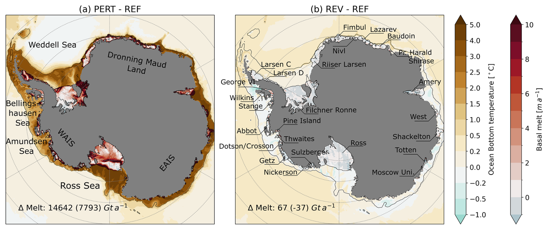
Figure 2 Ocean bottom temperature (blue to brown colour bar) and basal melt rate (blue to red colour bar) anomaly (a) due to the atmospheric perturbation (PERT minus REF, averaged from their 46th to 55th years), and (b) after removal of the atmospheric perturbation (REV averaged from its 61st to 70th year minus REF averaged from its 46th to 55th year). The differences in total basal melt between the two simulations are indicated in the lower left corners. Numbers in brackets are the melt differences estimated only beneath the non-vanished ice-shelf cells (h_ice > h_min).

The continental shelf becomes a warm-fresh type all around Antarctica, as defined in MJ2023, with a westward surface current above the shelf break and an eastward or near-zero current near the seafloor, favouring the intrusion of CDW (Fig. 3). These changes in shelf properties lead to a tenfold increase in average basal melt rates beneath the Antarctic ice shelves, from 1204 (REF) to 15 783 (PERT) Gt a⁻¹, consistent with the corresponding MJ2023 simulations (1182 to 13 572 Gt a⁻¹ over the same period).

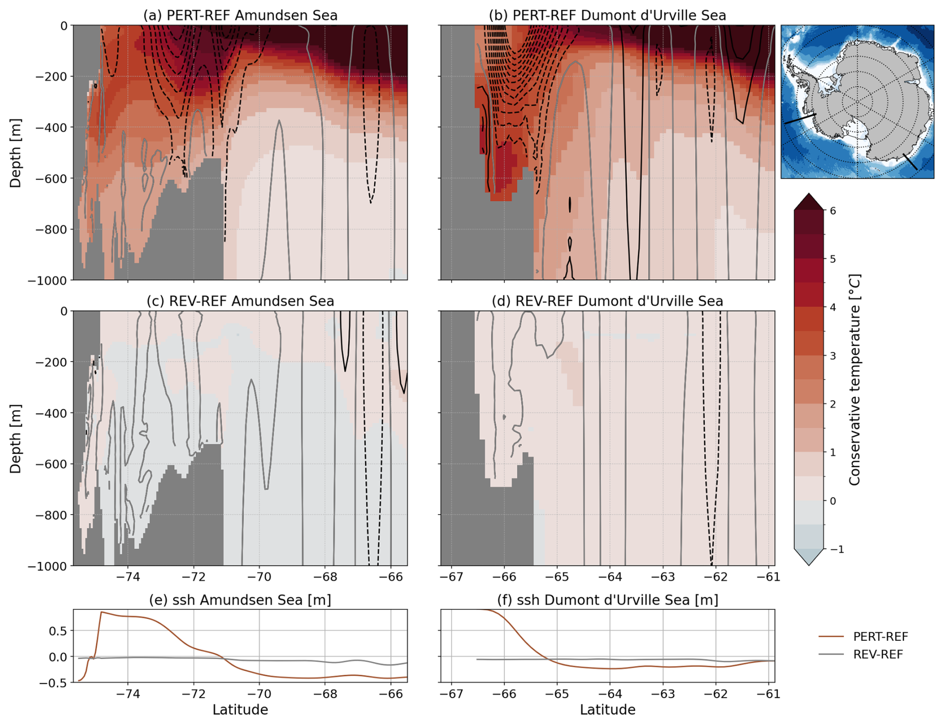
Figure 3 (a, c) Temperature differences along a vertical section across the Amundsen Sea: (a) Differences between PERT and REF and (c) between REV and REF. (b, d) Temperature differences along a cross-section across the Dumont d’Urville Sea: (b) Differences between PERT and REF and (d) Between REV and REF. The same years as in Fig. 2 are used to calculate these differences. The black contours show the zonal velocity differences every 5 cm s⁻¹ (dashed/solid lines for westward/eastward velocity differences), gray line for zero velocity difference. (e–f) Sea surface height difference profile along the corresponding sections between PERT and REF (brown) and REV and REF (gray).

Similar to MJ2023 REF, the mean basal mass loss in the coupled REF simulation (1204 Gt a⁻¹ over 2009–2018) is also consistent with observational estimates for Antarctica of 1325 ± 235 Gt a⁻¹ for the 2000s (Rignot et al., 2013) and of 965 ± 265 Gt a⁻¹ over 1992–2017 (Paolo et al., 2023). At the scale of individual ice shelves, the mean basal mass loss also generally matches observational estimates (Fig. 4). There are nonetheless some differences in ice-shelf basal melt rates between our coupled simulations and MJ2023 (Fig. 4). For the reference simulation, these differences are mainly observed at Getz and George VI. In MJ2023 REF, due to the absence of feedback between basal melt rates and ice-shelf draft depth in the presence of a strong ocean thermocline bias, the melt rate was much higher than observed for George VI. The melt rate bias for the Getz ice shelf in MJ2023 REF was such that the draft was artificially thinned to mitigate the impact of the ocean bias in front of the ice shelf. In this study, the feedback between the ocean and the ice sheet allows Elmer/Ice to rapidly adjust to a shallower ice draft, deviating from the initial inverse topography. As a result, parts of the ice-shelf draft stabilize in colder water, leading to more realistic melt rates with respect to the observational estimates of Rignot et al. (2013) (Fig. 4).

For the perturbed experiment, the first difference with MJ2023 PERT is that weaker melt rates are simulated beneath the inner part of ice shelves (because they thin in the coupled experiments, sometimes moving above the thermocline). This is compensated by stronger melt rates at the grounding line and a generally larger ice-shelf area due to grounding-line retreat (not shown). Notably, this compensation results in similar integrated melt rates between PERT and MJ2023 PERT only when both the ice shelf and pseudo-collapsed areas are considered; otherwise, PERT yields much weaker melt. It is worth noting that 49 % of the melt in the perturbed experiment occurs in the pseudo-collapsed areas where the ice shelf reaches the minimum thickness of 1 m allowed by Elmer/Ice (Figs. 2 and 4). The fraction of melt occurring in these pseudo-collapsed areas varies greatly from one ice shelf to another, e.g., 8 % for Filchner-Ronne and 91 % for Larsen D (Fig. 4). The impact of non-stop melting in the pseudo-collapsed areas is discussed in Sect. 5.

Another difference with MJ2023 is that the iceberg calving flux is now computed interactively and depends on ice-shelf thickness and velocity. In REF, the mean iceberg calving flux, estimated from the mean iceberg melt over the period, is 1125 Gt a⁻¹ over 2009–2018 (Fig. 6c). This iceberg calving flux, provided by Elmer/Ice, is consistent with the observational estimate of ice front flux by Rignot et al. (2013) (1325 Gt a⁻¹). Following the onset of the perturbation, the integrated iceberg melt initially increases sharply to 3620 Gt a⁻¹ in PERT, but subsequently decreases and stabilizes at a lower value of 535 Gt a⁻¹ (years 46–55). This response reflects the adjustment of the iceberg calving flux to the ice-sheet response to the perturbation: ice-shelf thinning caused by enhanced basal melting reduces the iceberg calving flux in our model formulation, while the associated increase in ice-shelf velocity is not sufficient to compensate for this effect.

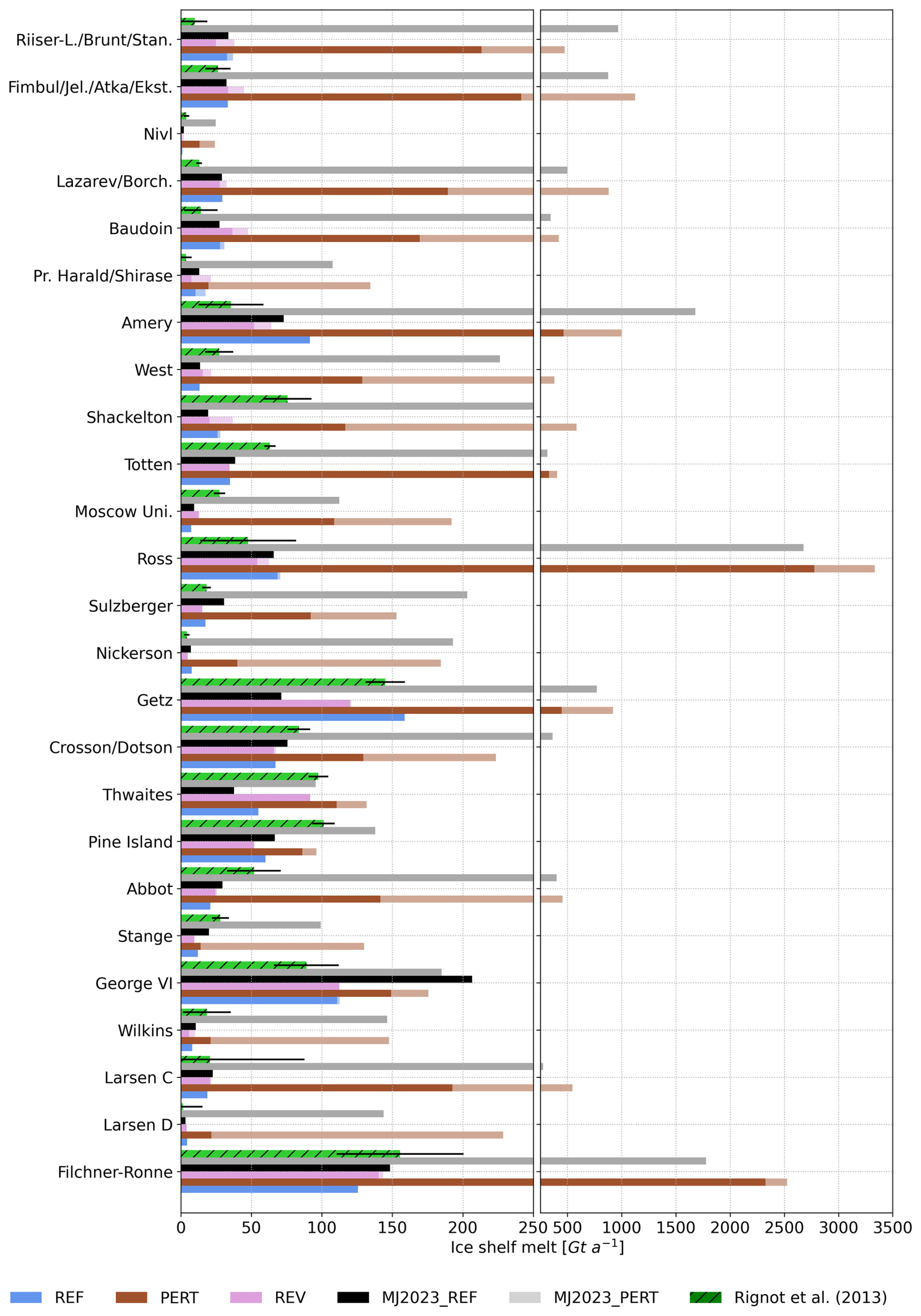
Figure 4 Total basal melt per ice shelf (in Gt a⁻¹) averaged over the last 10 years of each simulation in REF (blue), PERT (brown), REV (pink), MJ2023 REF (black), MJ2023 PERT (grey) and Rignot et al. (2013) (hashed green). For clarity, only ice shelves (or groups of ice shelves) larger than 4000 km² are represented (∼ 70 % of the total ice-shelf area, Rignot et al., 2013). The lighter parts of the bars indicate the contribution of the pseudo-collapsed area (h_ice ≤ 1 m). Location of each ice shelf is shown in Fig. 2b.

Ocean properties on the continental shelf appear to be entirely reversible within 70 years. Switching back to the reference atmospheric forcing is enough to restore sea-ice area (Fig. 5a) and brine rejection (Fig. 5b) to the reference state. This triggers the formation of new HSSW (Fig. 5c) that spreads on all former dense shelves, rebuilding shelf dense water and the density barrier that prevents intrusion of warm CDW (Fig. 3). The brine rejection also regenerates the cold winter surface mixed layer and the Antarctic Surface Water (AASW). These features are key to the formation of fresh shelves (Thompson et al., 2018). Furthermore, the CDW cools back to the reference value. This allows the Amundsen and Bellingshausen Seas to return to their present day properties (Fig. 3). Consequently, the end state of the reversibility experiment is very similar to the reference state (Fig. 2b). The reversal of ocean properties on various shelves begins immediately after the atmospheric forcing is reversed, as does the ice-shelf basal melt, and takes approximately 40 years to complete (Fig. 6a–b). The reversibility of iceberg melt is closely linked to the timescale required for iceberg calving to recover from the perturbation. In our model formulation, and under the fixed ice-front approximation, the iceberg calving flux is equal to the ice front flux, consequently its recovery follows the timescale of the ice sheet rather than that of the ocean. Returning to the REF iceberg melt state therefore takes more than 70 years (Fig. 6c), but the deficit remains limited and does not seem to affect the ocean reversibility.

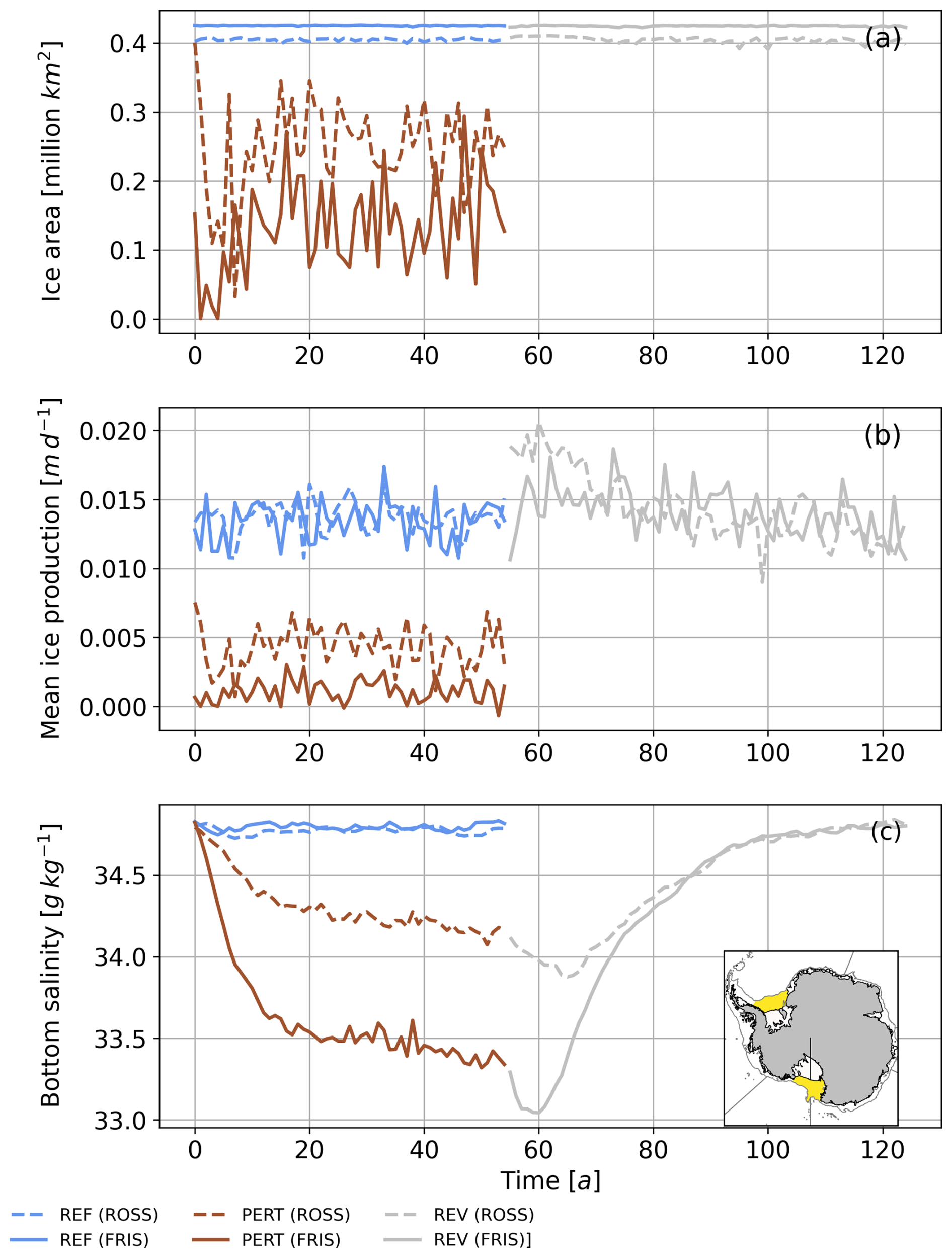
Figure 5 (a) Time series of sea-ice area, (b) mean sea-ice production, and (c) bottom salinity on the Ross and Filchner-Ronne continental shelves.

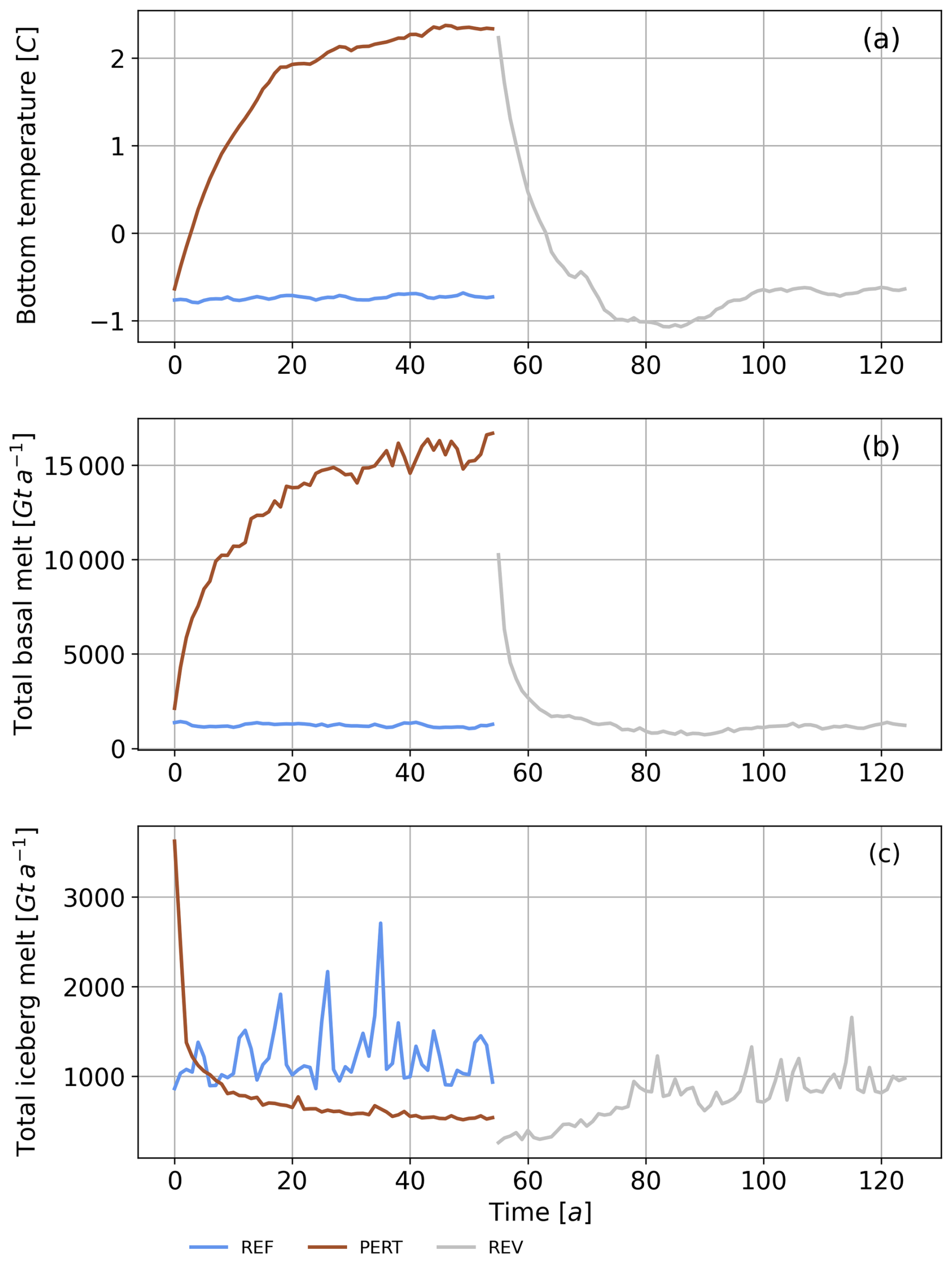
Figure 6 (a) Time series of bottom temperature averaged over the Antarctica continental shelf (bathymetry shallower than 1000 m), (b) integrated ice-shelf basal melt, and (c) integrated iceberg melt.

The integrated melt per ice shelf is reversible for most of the ice shelves (Fig. 4) and for Antarctica (an integrated difference of 67 Gt a⁻¹, i.e., ∼ 5 %, between REV and REF). This is a balance between the thinner ice shelves at the end of the coupled REV experiment, which tend to reduce the thermal forcing, and a larger ice-shelf area because the grounding line does not return to their original positions after 70 years (Fig. 7b). The abrupt increase in melting is not fully reversible beneath three ice shelves (Thwaites, Getz and Amery) for which noticeable differences are found between REV and REF (Fig. 4). Getz and Amery melt less after the reversibility experiment than in the reference. This is due to thinner ice shelves inducing lower thermal driving both due to the pressure dependence of the freezing point and to the displacement of the ice draft toward the cold surface layer. In these shallower ice shelves, melting may also be more influenced by near-surface processes, such as seasonal cycle of the surface water (Mode 3 melting; Jacobs et al., 1992), potentially further reducing basal melt rates compared to mode 1 (HSSW) or 2 (Getz). These changes outweigh the effects of the increase in ice-shelf area. In contrast, Thwaites melts more after the reversibility experiment because the grounding-line retreat exposes a large ice area to CDW (Fig. 8).

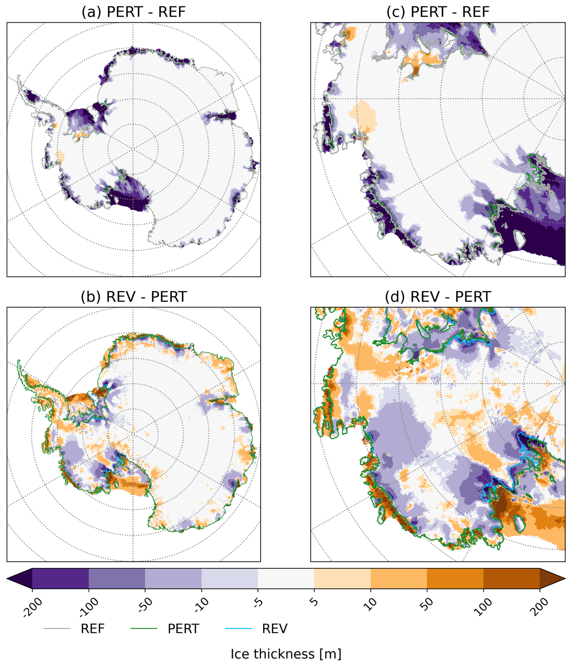
Figure 7 Ice thickness anomaly (a) after 55 years of atmospheric perturbation (PERT at year 55, i.e. at the end of the coupled PERT simulation) w.r.t. REF (year 55, i.e. at the end of the coupled REF simulation), and (b) after 70 more years of reversed atmospheric forcing (REV at year 70, i.e. at the end of the coupled REV simulation) w.r.t. PERT (year 55, i.e. at the end of the coupled PERT simulation). (c) and (d) are respectively zoomed-in views of (a) and (b). In grey, green and blue the grounding-line position in REF, PERT and REV, respectively.

3.2 Discussion on the ocean transition and its reversibility

As in MJ2023, our results indicate that transitions from cold to warm cavities do occur for all Antarctic ice shelves under conditions between the present-day climate and a plausible realisation of 2300 under SSP5-8.5. Our method is not appropriate for the identification of atmospheric thresholds that lead to abrupt warming in ice-shelf cavities under gradually changing atmospheric conditions. The relatively high resolution required to simulate a large number of ice shelves makes it computationally difficult to produce large ensemble of simulations, which would be required to address tipping points in a more systematic way, as done in Garbe et al. (2020) for the Antarctic Ice Sheet.

A new result is that transitions to a warm state appear to be reversible within 40 years for most shelves in our simulations (Fig. 6). It is important to stress that this was estimated by assuming that the atmospheric state can be reversed instantaneously, which is not realistic, and by assuming a fixed ice front. The potential impacts of ice-shelf collapse and evolving cavity geometry on ocean reversibility are discussed in Sect. 5. We nonetheless believe that these results are useful for understanding the climate system, as they indicate that the Southern Ocean itself may not contribute to making large climate transitions irreversible as it was suggested in previous work.

The reversibility of the Filchner-Ronne cold-to-warm transition reported in this study is consistent with Reese et al. (2026) and somewhat consistent with Haid et al. (2023), but differs from Hellmer et al. (2017) and Hazel and Stewart (2020), who identified a hysteresis behaviour (see introduction). The perturbation methods differ across these studies, so it is difficult to find an explanation for these differences. First, our findings do not rule out the existence of a hysteresis in the melt response to the atmospheric forcing, but if there is a hysteresis, it must be narrower than the perturbation that we impose. In this case, it would mean that our transitions jump from one side of the hysteresis to the other, hence appearing as reversible. Second, the tipping/reversal threshold is determined by the interplay between the activity of the Ronne ice-shelf polynya (Moorman et al., 2023; Saddier et al., 2026), basal melting beneath Filchner-Ronne (Hellmer et al., 2017), and advection from the westward coastal current (Hazel and Stewart, 2020; Bull et al., 2021). Therefore, any model bias or difference in the modelling setup may impact the tipping behaviour.

In particular, polynya activity plays a critical role by setting the dense shelf water density, which is the main driver of the density barrier preventing CDW from spreading onto the continental shelf (Naughten et al., 2021). This activity is strongly sensitive to the resolution and fidelity of atmospheric forcing. For example, reanalysis used in our study and in Haid et al. (2023) may represent this activity more accurately than in the coarse climate models used in Hellmer et al. (2017). Similarly, the properties of CDW in regional simulations, such as those in Hellmer et al. (2017) and Hazel and Stewart (2020), are highly sensitive to the choice of ocean lateral boundary conditions compared to the global ocean simulations used in our study and in Haid et al. (2023). These modeling choices affect the response of CDW to changes in atmospheric forcing and, consequently, its ability to intrude onto the continental shelf.

Very few studies have so far investigated ocean tipping points and their reversibility outside of Filchner-Ronne. Caillet et al. (2023) showed that surface buoyancy fluxes were the main drivers of multi-decadal transitions between cold and warm states in the Amundsen Sea. They did not identify any hysteresis in these long-term regime shifts, although their interannual transitions between cold periods and warmer periods can be interpreted as an indication of bi-stability (Moorman et al., 2023).

For the Ross Ice Shelf, a possible reversibility for large transitions is supported by paleo-proxies suggesting a warm-to-cold transition during the mid-Holocene (Lowry et al., 2024). The main suggested driver of such a transition is an increase in polynya activity, which leads to a strengthening of the HSSW formation, flooding the Ross shelf with cold water. This mechanism is similar to the one simulated in our reversibility experiment. However, reversibility may only apply to very large atmospheric shifts, such as the one applied in this study, and may not occur for smaller perturbations. Hysteresis effects, where the ocean remains in a warm state despite the cessation of perturbation, could emerge under more moderate perturbations, as demonstrated by Garbe et al. (2020) for the Antarctic Ice Sheet.

4 Ice-sheet tipping points

4.1 Results

Despite a geometry initialization from Bedmachine v2 and viscosity and friction fields derived from an inversion constrained by observed velocity (see Sect. 2.1.2), the model simulates a grounding-line flux of 1554 Gt a⁻¹, which is 25 % lower than the estimates of Rignot et al. (2013). Therefore, the mass trend for the same period (+1 Gt a⁻¹) is higher than the IMBIE estimate of −106 Gt a⁻¹ for 1995–2014 (Shepherd et al., 2018). This growing bias is quite common in ice-sheet models (Seroussi et al., 2020; Aschwanden et al., 2021) and arises from challenges in simulating the high melt rates observed at the grounding line with NEMO (MJ2023), the absence of ice-shelf front retreat and associated buttressing loss due to iceberg calving, the lack of evolving viscosity due to damage, or the omission of subglacial hydrology. However, since PERT and REV are analyzed relative to REF or REF_ext, these biases are unlikely to substantially affect the main conclusions of the analyses presented here.

To assess the response of individual ice drainage basins to the changes in oceanic conditions during the coupled perturbation (PERT) and reversibility (REV) experiments, as well as during the standalone ice-sheet extension (REV_ext), three variables are analysed: the flux at the grounding line, the integrated grounded area, which is used as a proxy for the grounding-line position, and the volume above flotation (VAF), which indicates the ice-sheet contribution to changes in sea level.

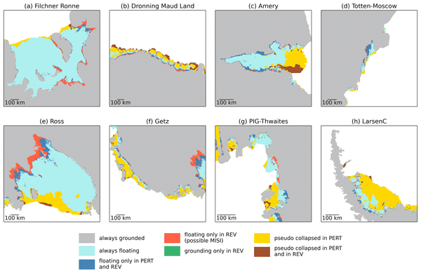
The strong increase in melt rates induced by the ocean in response to the atmospheric perturbations leads to a pronounced thinning of all ice shelves, exceeding 200 m in many places after 55 years (Fig. 7a). The extent of thinning is so severe that some ice shelves, such as Getz, Abbot, and Larsen, entirely reach a pseudo-collapsed state (yellow area in Fig. 8). At most locations, such ice-shelf thinning leads to a strong loss of buttressing (Fürst et al., 2016), which accelerates the upstream ice streams (not shown), resulting in a rapid increase in ice transport across the grounding line. The total ice flux across the grounding line in Antarctica nearly doubles in PERT compared to REF (Fig. 9a). This thinning also causes the retreat of grounding lines in all major basins, particularly for the Filchner-Ronne, Ross, Thwaites, and Dronning Maud Land ice shelves (Fig. 8).

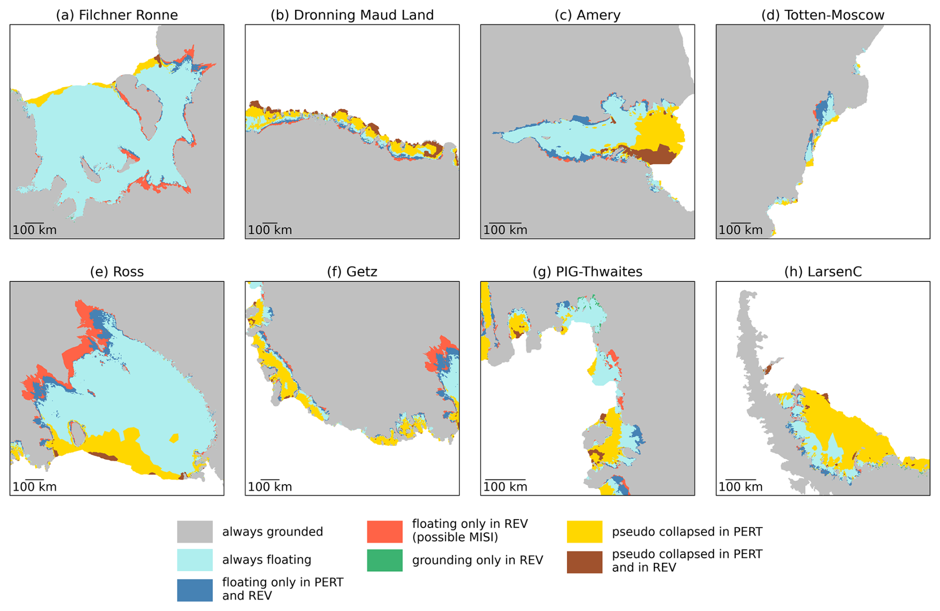
Figure 8 Area types (grounded, floating, and collapsed) at the end of REF, PERT, and REV. Gray (turquoise) represents areas that are always grounded (floating). Yellow (brown) indicates areas that are collapsed at the end of PERT (and remain collapsed at the end of REV). Blue (red) shows areas that become ungrounded during PERT (and stay ungrounded in REV). Green represents areas that are grounded only in REV.

The reversibility of the ice sheet is much more complex than that of the ocean due to the varying characteristics of the basins and the slower response time of the ice sheet to increased melt rates, which goes beyond the PERT and REV periods and motivated the extension through standalone simulations. After 70 years, REV exhibits locations thinner than at the end of PERT (Fig. 7c–d) where the grounding line has retreated beyond its original PERT position and does not re-advance even after ocean conditions revert to their original state (Figs. 7c, d and 8). This retreat of the grounding line beyond its position in PERT leads to reduced buttressing, accelerated ice flow, and dynamic thinning. These locations highlight ice sheets that may be susceptible to irreversible changes. After 500 years of simulation (encompassing the PERT, REV, and REV_ext phases), the East Antarctic sector, including the Enderby, Amery, Princess Elisabeth, Aurora Subglacial, and Wilkes Subglacial basins, shows signs of reversibility: ice flux at the grounding line rapidly returns to its reference value (Fig. 9a), the grounding line slowly re-advances toward its position in the reference simulation (Fig. 9b), and mass above flotation is gradually re-approaching the reference simulation (Fig. 9c). Other ice drainage basins, such as Filchner-Ronne, Dronning Maud Land (Baudouin, Fimbul and Coats), Ross and Amundsen show signs of instability: their mass above flotation keeps diverging after 500 years (Fig. 9c).

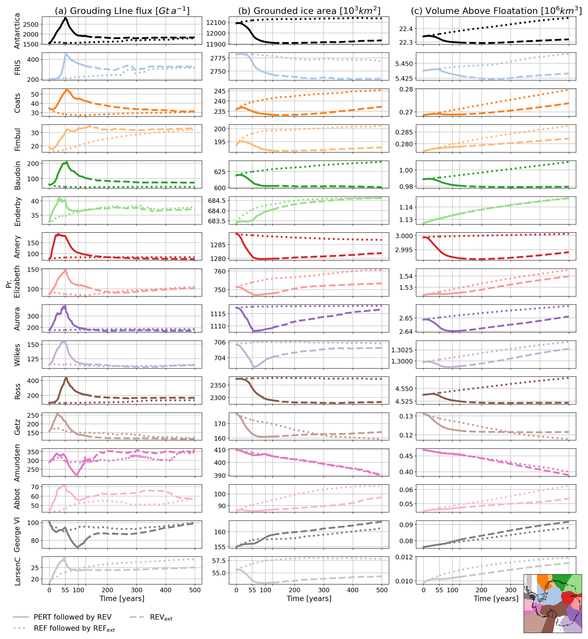
Figure 9 Time series of (a) grounding-line flux, (b) grounded ice area, (c) volume above flotation for the whole Antarctic ice sheet (black, upper panels) and individual ice drainage basins (see corresponding colours on the map in the lower right corner). Results are displayed for PERT and REV (solid line), REV_ext (dashed) and REF and its extension (dotted). Only the basins with grounding-line flux of more than 15 Gt a⁻¹ at the start of the simulations are represented.

However, by looking at individual streams, the picture is very contrasted. The instabilities of Filchner-Ronne, Dronning Maud Land, Ross, and Amundsen ice basins are driven by only a few streams (Fig. 10). Thwaites, Ice Streams A to E feeding the Ross Ice Shelf, Baudoin, Borchgrevink, Fimbul, and Riiser-Larsen feeding the Dronning Maud Land ice shelves and the Bailey, Slessor, and Institute ice streams feeding the Filchner-Ronne ice shelf continue to retreat despite the removal of the perturbation (see Fig. 10 for the locations). These streams also lose mass at a faster rate than in the reference simulation (Fig. 10).

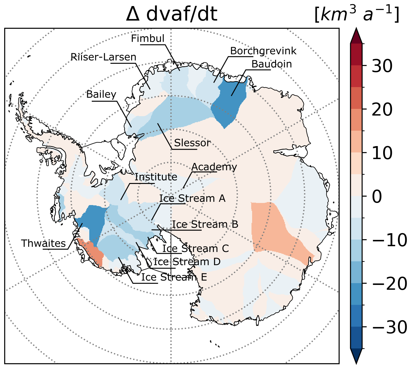
Figure 10 Difference in the rate of variation of VAF between REV and REF at the end of the simulation (year 500).

Nevertheless, when examining various indicators such as flux at the grounding line, grounding-line position, and VAF, it becomes evident that reversibility is dependent on both the timescale and the metrics used. With the exception of Thwaites, all the aforementioned ice streams show reversible fluxes at the grounding line over a timescale shorter than the 500-years period studied here (Fig. 11a), despite their continued mass loss relative to the REF_ext (Fig. 11c). For most of these ice streams, the grounding line continues to retreat inland for the first 200 years after the reversibility experiment began. However, a few of them continue to retreat inland until the end of the 500-year simulation (Ice Stream A and B in the Ross Basin, Thwaites Glacier, Institute ice streams in the Filchner-Ronne Basin, and Fimbul, Borchgrevink, and Baudouin ice streams in Dronning Maud Land). This indicates that these streams might have entered a self-sustained grounding-line retreat. The others eventually stabilize or readvance.

Figure 11 (a) Anomaly of grounding-line flux in PERT and then REV with respect to REF. (b) as (a) but for the grounded ice area (proxy for grounding-line advance or retreat). (c) as (a) but for the VAF.

The reversibility of the ice shelves is also slower than the 70-year duration of the REV phase. Notably, certain areas remain in a pseudo-collapsed state even after the reversibility phase (brown areas in Fig. 8). These regions, where the ice thickness is reduced to 1 m, are particularly prone to regrowth (Fig. 7c, d), more so than if a complete collapse had occurred, as they may experience positive snow accumulation and frazil ice formation. The fact that these areas do not exhibit significant regrowth suggests that their growth by ice advection is too slow to counterbalance the basal melt. Furthermore, even for areas that always remain afloat (turquoise areas in Fig. 8), the recovery of ice-shelf thickness is slower than the REV timescale. Figure 7 shows that many ice shelves lose more than 200 m of ice and recover only between 5 and 100 m at the front.

4.2 Discussion

Our experimental framework, while not designed to identify specific thresholds for ocean warming that trigger regime shifts in ice-sheet dynamics, demonstrates that a short (55-year) but intense atmospheric perturbation over the ocean can induce instability in certain Antarctic ice basins. Notably, these instabilities persist as irreversible retreat over the 500-year timescale of our study and likely beyond for specific ice catchment basins and ice streams, despite the ocean returning to present-day conditions within 40 years. This underscores the asymmetry in reversibility between ocean and ice-sheet responses, a critical insight for understanding long-term climate commitments.

At the basin scale, the integrated trends in grounding-line positions reveal that most basins either re-advance immediately or after a delay following the perturbation. However, some basins, such as the Wilkes Subglacial Basin, are known for their potential instability. Mengel and Levermann (2014), using ocean temperature anomalies of 1.0–2.5 °C applied for 200–800 years, demonstrated that the removal of a specific coastal ice volume, acting as a protective “ice plug” of 60–80 mm sea-level equivalent (22 200–29 600 Gt), would destabilize the entire Wilkes Basin. Similarly, Garbe et al. (2020), who applied millennial-scale temperature perturbations (increases of > 10 °C at a rate of 10⁻⁴ °C a⁻¹), show that sectors such as the Wilkes and Aurora basins can exhibit irreversible retreat under such strong and sustained forcing. In contrast, our simulations show only a modest ice loss (∼ 1200 Gt), far below the ∼ 30 000 Gt required to remove the protective “ice plug” (Mengel and Levermann, 2014). This discrepancy likely arises from the short duration of our perturbation, which may not have been sufficient to reach the tipping point. Similarly, the Aurora Subglacial Basin, another region prone to irreversible retreat (Garbe et al., 2020), shows no signs of instability in our simulations, further suggesting that longer or stronger perturbations are necessary to cross critical thresholds.

Our study highlights that basin-scale analyses alone are insufficient to assess ice-sheet stability. Within individual basins, specific ice streams, such as Baudouin, Borchgrevink, Institute, Jutulstraumen, Thwaites, Mercer, and Whillans, continue to retreat even after 350 years of reversibility. This indicates that stability assessments must account for the behaviour of individual ice streams, as their responses can diverge significantly from basin-wide trends.

The reversibility of grounding-line positions occurs over longer timescales compared to grounding-line flux, consistent with findings from standalone ice-sheet models (Hill et al., 2023). Our simulations also align with grounding line retreat patterns observed in the UKESM Earth System Model (Siahaan et al., 2022) and other standalone models (Seroussi et al., 2024; Reese et al., 2023). However, a notable exception is the behaviour of Pine Island Glacier (PIG).

Favier et al. (2014) demonstrated that PIG is on the edge of an irreversible retreat. Other studies also support the fact that PIG may be unstable under various forcing (Seroussi et al., 2024; Reese et al., 2023). However, in our simulations, PIG shows no signs of retreat – neither during the perturbation nor during the reversibility phase. Instead, the grounding line advances onto the latest subglacial ridge. This behaviour in Elmer/Ice is consistent with Hill et al. (2023) and is a longstanding issue. One likely reason is the insufficient melt rates at the grounding-line. As discussed in MJ2023, this underestimation may be due to a lack of horizontal and vertical resolution in this area (Jourdain et al., 2022) as well as the absence of subglacial runoff (Nakayama et al., 2021), preventing the grounding line from retreating.

In contrast to PIG, the nearby Thwaites Glacier exhibits irreversible inland retreat. Gudmundsson et al. (2023) demonstrated that Thwaites's behaviour was complex, with limited sensitivity to ice-shelf collapse at century timescales, with minimal SLR contribution due to weak buttressing from its current ice-shelf configuration. In addition, their work highlighted a strong sensitivity to the friction law, ice-sheet model, and model setup, as well as spatial heterogeneity in the response. Thwaites East gains mass after ice-shelf removal, while Thwaites West loses mass, reflecting contrasting regional dynamics.

In our simulations, Thwaites initially responds with limited grounding-line retreat and VAF changes over the first 100 years, consistent with Gudmundsson et al. (2023). However, beyond this period, the grounding line retreats inland, triggering rapid ice flux acceleration and VAF decline. This nonlinear transition suggests that Thwaites may remain stable under short-term perturbations but could undergo accelerated retreat once critical thresholds are surpassed, aligning with Joughin et al. (2014). While the exact conditions for triggering such instability are beyond our scope, our results underscore the potential for delayed but significant destabilization in response to ocean forcing perturbations.

Direct comparisons between the various studies remain challenging due to differences in experimental setups, including forcing scenarios, model configurations, and timescales. Nonetheless, our findings contribute to the growing evidence that ice-sheet responses to climate perturbations are highly nonlinear, with critical implications for future projections.

5 General discussion

Although our model provides an advanced representation of ocean–ice-shelf interactions, the high computational cost imposes several limitations. Three key aspects are particularly affected: (i) the spin-up procedure with standalone components does not achieve a perfect balance between the different components of the coupled model, (ii) the use of fixed melt rates during the extended simulation period may limit the model’s ability to capture long-term feedbacks between ice-shelf geometry and melt rates, especially in regions with a strong thermocline (as in Getz ice shelf, for example), and (iii) the computational constraints prevent a systematic exploration of tipping points through multiple small perturbation experiments and reversibility analyses.

There are also caveats related to structural limitations of our models and setup. Evolving ice damage and iceberg calving in the ice-sheet component may also increase the irreversibility of ice acceleration and thinning. Here, ice damage and ice front position are assumed to be constant. With a prognostic iceberg calving law, the net response would depend on multiple processes, such as ice-shelf thinning, flow acceleration, deformation and damage, and the evolution of the ice front (Wilner et al., 2023). The iceberg calving response simulated in PERT and REV, including the recovery timescale of more than 70-year, should therefore be regarded as characteristic of our model formulation rather than as a robust estimate of the physical response or recovery timescale of iceberg calving. Furthermore, our approach in the coupling framework has been to keep a minimum ice-shelf thickness of 1 m, while still calculating melt rates in the ocean model. The overestimated meltwater flux may amplify the ocean warming at depth (Bett et al., 2020; Caillet et al., 2023), but does not prevent reversibility. In our study, under present-day surface mass balance, ice shelves remain safe from hydrofracturing. Using a surface mass balance typical of 2300, as it is done for the ocean, may lead to hydrofracturing and larger ice-shelf collapse (Jourdain et al., 2025), potentially triggering Marine Ice Cliff Instability (MICI; Pollard et al., 2015), a proposed mechanism whose relevance for Antarctic ice-sheet evolution remains under debate (e.g. Morlighem et al., 2024).

Our study focuses on ice-ocean interactions and does not include a fully coupled ocean–atmosphere–ice-sheet system with evolving land, ocean, and ice-sheet fractions seen by the atmosphere, so we cannot quantitatively assess how atmospheric forcing over newly ice-free regions would influence the ocean–ice-sheet system’s reversibility. In the absence of a moving ice front, for stability reasons, we impose a minimum thickness of 1 m, which maintains a thin ice layer that isolates the ocean from direct atmospheric forcing compared to open water, while also facilitating regrowth under cold conditions compared to a real ice-shelf front that would need to readvance progressively.

Our perturbation induces retreat of most ice-shelf fronts (Amery, Ross and FRIS) or even pseudo-collapse of some ice shelves (e.g., Getz, Dotson/Crosson, Abbot, Cosgrove, the Larsens, ...). Such changes, in a fully coupled system, would result in a reduced ice-shelf area and more open water exposed to the atmosphere, affecting ocean heat transport into the ice-shelf cavities (Bradley et al., 2022), with significant uncertainties related to the presence of sea ice, icebergs and polynyas in deglaciated areas.

6 Conclusions

In this study, we introduced a new global coupled ocean–ice-sheet model, inspired by the idealized work of Favier et al. (2019). This work represents a preliminary step toward the future integration of the Elmer/Ice ice-sheet model into an Earth System Model.

To investigate whether regime shifts in Antarctic shelf waters can trigger glaciological tipping points in the Antarctic Ice Sheet, we used an approach similar to that of MJ2023, but within a global coupled ocean–ice-sheet framework instead of an ocean only model. To achieve this, we applied a strong and abrupt perturbation to atmospheric conditions typical of the year 2300 under the SSP5-8.5 scenario (MJ2023), over the ocean for 55 years. Following this perturbation, we conducted an abrupt reversibility experiment, returning to present-day conditions for 70 years.

Consistent with the forced simulation results of MJ2023, our perturbed simulations reveal that the entire Antarctic continental shelf experiences substantial warming within the first two decades of perturbation, with several additional decades required for the largest ice-shelf cavities to adjust. In the absence of HSSW production, the intrusion of CDW onto the formerly cold continental shelves of the Ross, Weddell, and East Antarctica regions becomes more pronounced. These changes in oceanic properties lead to a significant increase in ice-shelf melt rates, with total basal mass loss escalating from 1200 to 15 800 Gt a⁻¹ after 55 years of perturbation.

The reversibility experiment demonstrated that all Antarctic shelf waters are capable of reversing to their original state within a relatively short period under the fixed ice shelf front condition. The primary mechanism identified is the resumption of convection due to brine formation when returning to present-day conditions. This leads to the formation of HSSW, spreading across the shelves and preventing CDW intrusion. Furthermore, the brine rejection facilitates the rebuilding of the surface cold mixed layer, and AASW. The northward migration of winds upon returning to present-day conditions contributes to restoring the typical fresh shelves.

As expected, the substantial increase in basal melt rates in the perturbation leads to the thinning of ice shelves, acceleration of ice streams, and retreat of ice-sheet grounding lines in most sectors. Additionally, several ice shelves (including the Larsen, Abbot, Cosgrove, Dotson/Crosson, Getz, and others) have experienced pseudo-collapse (1 m capping on ice-shelf thickness). When atmospheric conditions are reverted to present-day levels, grounding-line flux begins to decrease, and grounding-line positions start advancing toward their reference state in many ice drainage basins and streams. However, this reversibility process is much slower for the ice sheet than for the ocean, taking more than 100 years for grounding-line flux and more than 500 years for grounding-line positions to stabilize. We have identified 14 ice streams, primarily in the Ross, Amundsen, Filchner, Ronne, and Dronning Maud Land basins, that appear to undergo irreversible retreat (indicated by a growing difference in VAF between the reference and reversibility experiments over time). These findings align with Reese et al. (2023), though the reversibility of these streams depends significantly on the metrics and timescales considered.

Overall, all Antarctic ice-shelf cavities can switch to warm conditions at some level of global warming, triggering a strong response in ice-sheet dynamics. This study confirms the potential for irreversible Antarctic ice-sheet mass loss, pointing out that this behaviour is related to a small number of ice streams. In our modelling framework, we have not identified circumstances in which an irreversible change in the ice landscape would cause the ocean to tip to a different stable state.

However, this conclusion must be interpreted with caution. The fixed ice-front assumption used in our modeling framework prevents us from capturing the feedbacks associated with ice-shelf weakening or collapse, open-ocean exposure, and atmospheric interactions that would occur in a fully coupled system. A reduced ice-shelf area or ice-shelf collapse should increase the ocean surface seen by the atmosphere, which may enhance sea-ice formation and brine rejection or limit CDW intrusions, potentially favouring ocean reversibility. However, the associated atmosphere warming over the newly exposed ocean is unknown and may suppress the enhanced sea-ice formation. This highlights the need for fully coupled ocean–atmosphere–ice-sheet models to realistically assess the system’s response to perturbations and the potential for cascading feedbacks.

Appendix A

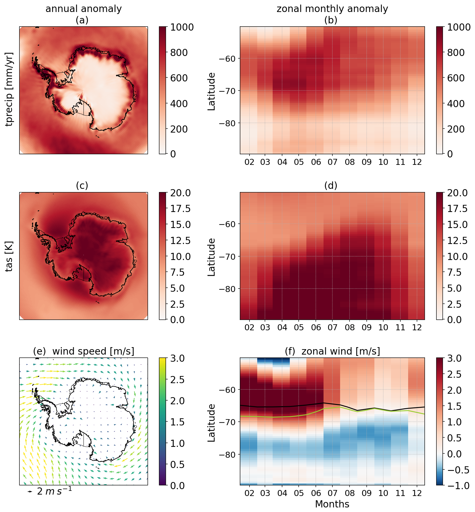
Figure A1 Maps of annual mean anomalies (left) and monthly-mean zonal-mean anomalies (right) for (a, b) total precipitation and (c, d) near surface air temperature, (e) near surface wind curl and wind anomalies (arrows), (f) near surface zonal wind. In (e) and (f), the blue line is the position of the zero zonal wind in the JRA reanalysis, and the brown line is the equivalent for the perturbed wind. Figure from MJ2023.

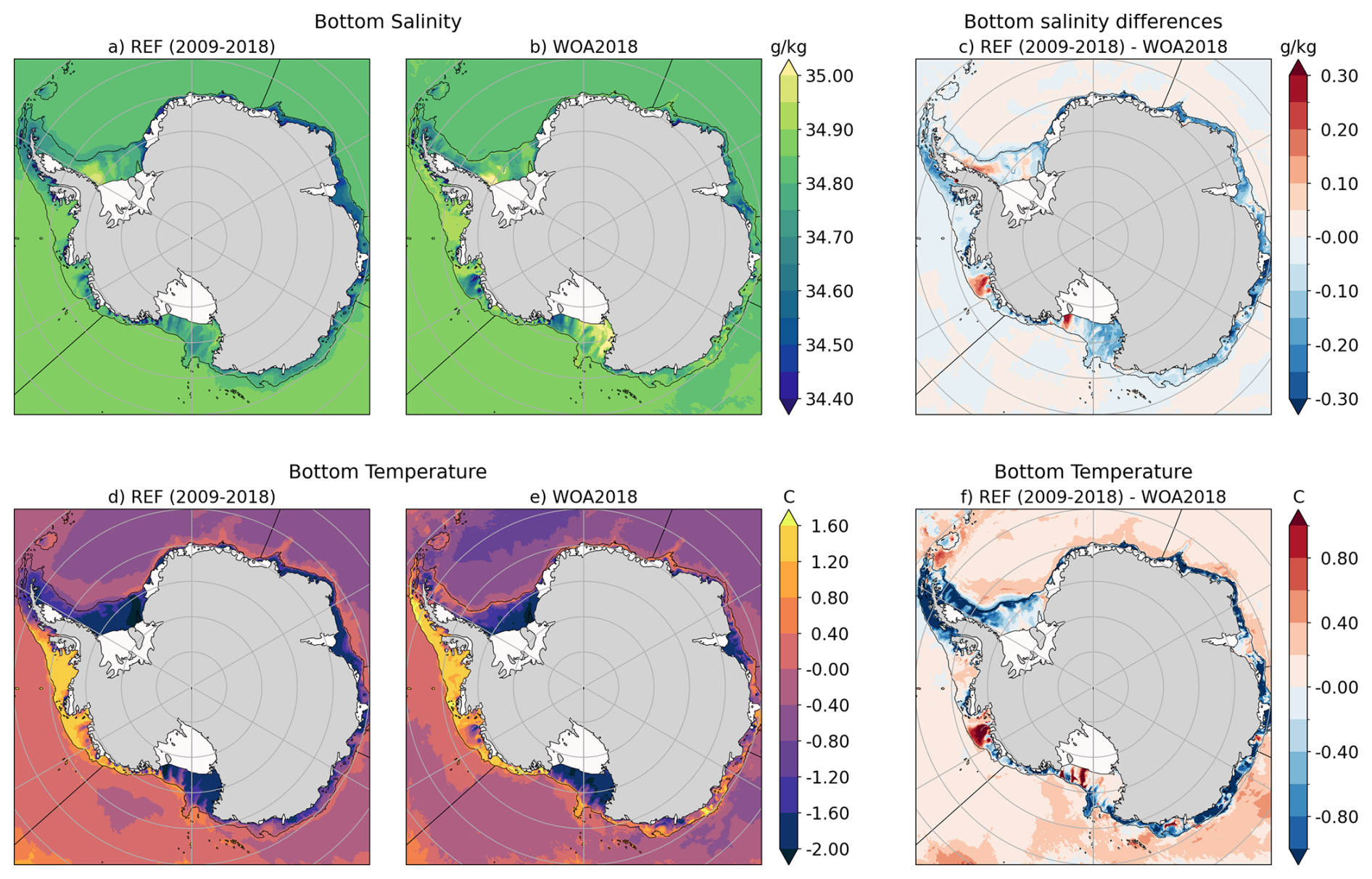
Figure A2 (a, b, c) Climatological bottom absolute salinity in (a) REF, (b) WOA2018 (Locarnini et al., 2018; Zweng et al., 2019), and (c) the difference REF-WOA2018. (d, e, f) Climatological conservative temperature in (d) REF, (e) WOA2018, and (f) the difference.