GlaUnTI: a hybrid physics–machine learning model enables transferable glacier surface mass balance estimation

Glacier surface mass balance (SMB) is a key climate indicator and a central driver of glacier change. Direct SMB observations remain sparse and unevenly distributed. Hence, transferable SMB models are essential for large-scale assessments and projections. Here, we propose the GLAcier-UNiversal Temperature Index model (GlaUnTI) for this purpose. This hybrid physics–machine learning model modifies a fully differentiable temperature index (TI) SMB model by introducing a shallow convolutional neural corrector. It learns spatially and temporally varying adjustments to a small set of physically interpretable TI parameters, using glacier geometry and aggregated climate information. We calibrate four models – a basic TI model, a purely data-driven recurrent neural network with no physical inductive bias and two GlaUnTI variants, with and without glacier facies maps as predictors – using a dataset of 65 European glaciers spanning 1995–2024 and covering the Alps, Scandinavia, Iceland, Svalbard and the Pyrenees. Their spatial transferability is evaluated on a held-out, spatially independent test subset of 13 glaciers across climatically and geometrically contrasting European regions. The evaluation uses 793/756/314 (annual/winter/summer) point SMB measurements and 312/235/233 glacier-wide SMB estimates. On the test glaciers, the baseline TI model achieves annual point-level performance with r=0.854 and an RMSE equal to 1.707 m w.e. With GlaUnTI, r increases to 0.940 and the RMSE reduces to 1.068 m w.e. At the glacier-wide scale, the baseline TI model attains an r equal to 0.606 and an RMSE of 0.805 m w.e. With GlaUnTI, r increases to 0.700 and the RMSE reduces to 0.627 m w.e. Including glacier facies maps from the end of the ablation season to the corrector yields moderate benefits in glacier-wide summer (11.0 %) and annual (12.2 %) SMB estimates. In contrast, the purely data-driven baseline model overall shows the weakest spatial transferability. Beyond modelling accuracy, end-to-end differentiability enables efficient gradient-based calibration, transfer learning, inverse optimisation of effective forcing perturbations, formal model explainability and propagation of forcing-driven aleatoric uncertainty through long SMB trajectories. These results demonstrate that parameter-corrected hybrid models improve SMB transferability across diverse climate regimes while preserving a physically grounded structure, suitable for integration into broader glacier evolution workflows and for informing climate-related policies.

1 Introduction

Glaciers are recognised as an essential climate variable (ECV) due to their sensitivity to atmospheric forcing and their integral role in the climate system, sea-level rise and regional water resources (GCOS, 2022; Zemp et al., 2019; Fox et al., 2024; Zemp et al., 2025). Changes in glacier surface mass balance (SMB), i.e. the net result of accumulation and ablation at the glacier surface, provide a direct and physically interpretable measure of glacier–climate interactions and are therefore a key ECV product (GCOS, 2022). Long-term SMB records underpin assessments of climate variability and change, support the attribution of observed glacier retreat and serve as critical inputs to glacier evolution and sea-level projections (Marzeion et al., 2012; Rounce et al., 2023). However, direct SMB observations remain sparse and unevenly distributed in space and time, particularly outside a small number of well-monitored regions (WGMS, 2021). Hence, robust modelling of SMB is essential to bridge observational gaps, enable consistent large-scale assessments and support the development of rigorous glacier projections under past and future climate conditions.

Temperature index (TI) models represent a class of mechanistic SMB models with a strong physical inductive bias in which melt is parameterised as a function of near-surface air temperature, typically combined with precipitation-based accumulation schemes. Conceptually, TI models can be viewed as simplified energy balance formulations: air temperature acts as a proxy for the net effect of turbulent heat fluxes and radiative forcing at the glacier surface (Ohmura, 2001; Hock, 2003). While full surface energy balance models explicitly resolve individual flux components such as shortwave and longwave radiation, sensible and latent heat fluxes, they require detailed meteorological forcing that is rarely available at large spatial scales (Hock, 2005; Pellicciotti et al., 2012). In contrast, TI models rely on temperature and precipitation time series and, hence, trade physical completeness for scalability, exploiting the well-established correlation between air temperature and melt energy, which has been shown to capture a substantial fraction of observed melt variability across climatic regimes (Braithwaite and Olesen, 1989; Hock, 2003). TI models commonly distinguish snow and ice melt using separate degree day factors (DDFs), reflecting their contrasting albedo and energy absorption characteristics and improving melt representation across seasonal and facies transitions (Braithwaite and Olesen, 1989; Hock, 2003). As a result of the balance between physical interpretability and data efficiency, TI models have become a standard backbone for regional and global glacier SMB and evolution studies (Marzeion et al., 2012; Huss and Hock, 2015; Zekollari et al., 2019; Rounce et al., 2023; Zekollari et al., 2024).

Despite their widespread use, the predictive accuracy of TI models depends critically on the calibration of a small number of empirical parameters, which are most often estimated independently for individual glaciers using local in situ or geodetic mass balance observations (Hock, 2003; Rounce et al., 2023). When geodetic datasets are used, DDFs and precipitation factors are commonly tuned, typically through grid search, so that the simulated glacier-wide cumulative mass balance matches the geodetic estimate over the survey period. This glacier-specific calibration limits the transferability of TI parameter sets across glaciers and climate regimes, challenging the “one model works everywhere” paradigm. Moreover, global geodetic mass balance products can be noisy at the individual glacier scale and represent an integrated mass change signal that is not strictly equivalent to SMB (Fischer, 2011). To address parameter uncertainty and reduce reliance on per-glacier tuning, Bayesian inference has been introduced into large-scale glacier evolution modelling, enabling joint estimation of melt factors, temperature bias and precipitation scaling while quantifying uncertainties from geodetic observations (Rounce et al., 2020). Bayesian methods have also been applied to investigate how observations with different temporal resolutions constrain TI model parameters across a sample of Norwegian glaciers, demonstrating sensitivity of posterior parameter distributions to seasonal versus annual data (Sjursen et al., 2023). More advanced strategies are emerging, including ensemble-based data assimilation approaches that combine multiple observational constraints (e.g., albedo and snow depth) to reduce uncertainty in mass balance estimates across glacier zones (Cao et al., 2025). In parallel, machine learning methods have been developed to learn transferable relationships from sparse SMB observations, with models such as XGBoost demonstrating improved generalisation to unmonitored glaciers (van der Meer et al., 2025; Sjursen et al., 2025). Related work by Bolibar et al. (2020) used a neural network to reconstruct annual glacier-wide SMB for French Alpine glaciers from climate and topographical predictors, highlighting the utility of auxiliary data beyond climatic variables alone. Collectively, these probabilistic and data-driven frameworks highlight the limitations of fixed, glacier-specific TI parameterisations and the ongoing efforts to build models that retain process understanding while improving transferability across heterogeneous glaciers.

Hybrid physics–machine learning modelling seeks to combine the extrapolative power of physics-based models with the flexibility of statistical learners by learning correction terms to compensate for structural error (Reichstein et al., 2019), embedding neural components inside governing equations (Rackauckas et al., 2021) and regularising training with physics-informed losses (Beucler et al., 2021) so that predictions remain consistent and trustworthy outside the training distribution. In glaciology, Jouvet and Cordonnier (2023) introduced physics-informed neural network emulators for glacier ice flow that are trained by minimising the energy associated with the ice flow model without requiring reference solution data, and Jouvet (2023) employed similar emulators for efficient GPU-accelerated inversion of Stokes ice flow models. Bolibar et al. (2023) introduced universal differential equations for glacier ice flow modelling, in which a neural network is embedded within a shallow-ice approximation to learn the variability of Glen's creep parameter among heterogeneous glaciers while preserving the form of the dynamics equations. Closely related physics-guided methods have been developed across Earth system sciences. Analogous embedded neural networks have been implemented within hydrological rainfall–runoff models to refine selected process parameterisations, keeping the overall structure intact and achieving accuracies comparable to the state-of-the-art deep learning models (Li et al., 2023). Physics-guided neural networks explicitly use process-model outputs as additional inputs and add physics-based loss terms to penalise violations of known constraints, improving generalisation and consistency relative to purely data-driven models in lake temperature profile modelling (Jia et al., 2021; Daw et al., 2021). This body of work motivates hybrid modelling, in which physical models are systematically refined using data-driven components, particularly in settings where observations are sparse and heterogeneity is pronounced.

In this study, we propose a method for large-scale SMB modelling that augments a physically-based, auto-differentiable TI model with data-driven parameter corrections derived from deep learning. The method first fits a single global TI model and then employs a shallow fully convolutional network to learn adjustment terms that account for spatially and temporally varying glacier-specific biases while keeping the physical structure intact. It is calibrated and evaluated on a pan-European dataset of 78 glaciers over 1995–2024, combining in situ point SMB measurements, glacier-wide SMB estimates, gridded elevation products and reanalysis-based climate forcing. Additionally, ensuring that the model is autodiff-friendly (i.e. implemented within an automatic differentiation framework so that gradients with respect to parameters and inputs are readily available) results in efficient and straightforward transfer learning, inverse optimisation, input attribution and aleatoric uncertainty estimation (Appendix A).

2 Study area

Our study area comprises 78 glaciers distributed across five European regions – the European Alps (38 glaciers), Scandinavia (21), Svalbard (9), Iceland (8) and the Pyrenees (2). In recent decades, glaciers across these study regions have shown persistently negative balances. In the European Alps and Pyrenees, regional geodetic assessments indicate mean losses of about $-\mathrm{0.74}\mathrm{m}\mathrm{w}.\mathrm{e}.{\mathrm{a}}^{-\mathrm{1}}$ for 2000–2016 (Davaze et al., 2020) and $-\mathrm{0.59}\mathrm{m}\mathrm{w}.\mathrm{e}.{\mathrm{a}}^{-\mathrm{1}}$ for 2011–2020 (Vidaller et al., 2021), respectively. Typical mass balance magnitudes of order $-\mathrm{1}\mathrm{m}\mathrm{w}.\mathrm{e}.{\mathrm{a}}^{-\mathrm{1}}$ were observed in Iceland for 1994–2019 (Aðalgeirsdóttir et al., 2020) and around $-\mathrm{0.21}\mathrm{m}\mathrm{w}.\mathrm{e}.{\mathrm{a}}^{-\mathrm{1}}$ in Svalbard for 2000–2019 (Schuler et al., 2020), consistent with generally negative mass balance in Scandinavia since 2000 (Andreassen et al., 2020) and recent global assessments of glacier mass loss in the last decades (Hugonnet et al., 2021; Zemp et al., 2025). Figure 1 shows the spatial distribution of the glaciers included in this study. The selected glaciers span a wide range of climatic settings, sizes and elevations, from maritime glaciers in Scandinavia and Iceland to more continental glaciers in the Alps and High Arctic conditions in Svalbard. The analysis covers the period 1995–2024. This heterogeneous sample reflects the uneven availability of glaciological observations in Europe and is deliberately chosen to test the transferability of SMB models across contrasting climate regimes, glacier geometries and surface conditions.

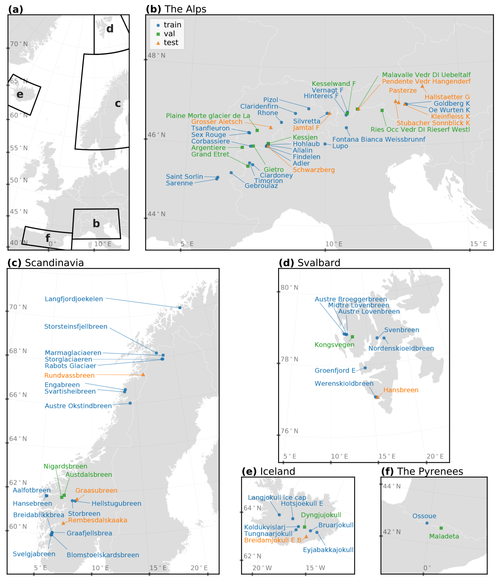
Figure 1 Glaciers of interest: (a) overview of the study area, (b) the Alps, (c) Scandinavia, (d) Svalbard, (e) Iceland and (f) the Pyrenees. The assignment of glaciers to training (blue circles), validation (green squares) and test (orange triangles) subsets is described in Sect. 4.4.

3 Datasets

We compile a set of observational datasets to constrain, force and evaluate our SMB modelling. Surface mass balance measurements from multiple monitoring programmes and regional archives provide the reference information for calibration and evaluation. Daily near-surface air temperature and precipitation form the minimal forcing required to run a TI model. In addition, we incorporate time-varying glacier geometry through annual estimates of surface elevations and glacier outlines. This geometry is based on observations rather than being simulated with an ice-flow model, providing an observationally constrained basis for SMB modelling without explicitly modelling ice dynamics. Finally, glacier facies maps derived from optical satellite imagery at the end of the ablation season are included where available as an additional descriptor of surface conditions. Jointly, the geometry- and surface-related datasets complement the climatic forcing by providing spatial context that allows glacier-specific biases to be assimilated as auxiliary information within the hybrid modelling. The following subsections describe each dataset in detail.

3.1 SMB data

We collected SMB data from several sources, including the World Glacier Monitoring Service (WGMS, 2021), the Glacier Monitoring Switzerland (GLAMOS, 2024), the Norwegian Water Resources and Energy Directorate (Elvehøy et al., 2025), CRYOBS-CLIM (, ) and the Iceland Glacier Web Portal (Icelandic Glaciers, 2025). For two glaciers in Svalbard, Austre Lovenbreen and Svenbreen, in situ SMB measurements were provided by the responsible investigators (Florian Tolle, personal communication, 2025; Jakub Małecki, personal communication, 2025) and consist of point measurements collected using the glaciological method. We harmonised all data to be largely compatible with the WGMS format. We distinguish between point SMB measurements, which are direct glaciological observations, and glacier-wide SMB estimates, which are derived by the corresponding monitoring programmes through spatial extrapolation of the glaciological observations over the glacier area. The latter are therefore used here as a weak constraint rather than as direct measurements in our modelling framework. All point measurements document the name of the glacier, the hydrological year of measurement, the geographical coordinates of the point, the balance value in m w.e., the balance type code (annual, winter or summer), and the begin and end dates of the measurement period. All glacier-wide estimates contain the name of the glacier, the hydrological year of the estimate, the annual balance in m w.e. and two dates defining the span of the hydrological year. Missing dates for glacier-wide estimates were imputed from the dates of adjacent year campaigns or, where possible, from corresponding point measurements. Any point-level or glacier-wide record missing at least one of these required fields was discarded. Glacier-wide estimates also contain optional fields – winter balance, summer balance and the end date of winter – for which missing values were allowed. In total, we compiled 10 483/15 421/3482 (annual/winter/summer) point measurements and 1637/1278/1279 glacier-wide estimates for the 30-year study period.

3.2 Elevation models

We used glacier surface elevation estimates and their associated uncertainty from Hugonnet et al. (2021), provided at 100 m spatial resolution. We extracted the elevation estimates referenced to the 30 September for each year, corresponding to the end of the hydrological year. These data are available for the period 2000–2019 and were used as the primary elevation product for our study. The elevation time series contains spatial voids (missing values), whose extent varies between glaciers due to data gaps in the underlying stereo-photogrammetric observations. To obtain spatially complete elevation fields while preserving realistic uncertainty estimates, we implemented a data-driven void imputation procedure (see Appendix B for the algorithmic description). Elevations outside the 2000–2019 observation window were extended to cover 1995–2024 by applying a quadratic fit in time independently at each grid cell. To assess the sensitivity to the elevation extrapolation, we repeated our subsequent analysis using backfilled elevations outside the 2000–2019 observation period (i.e., holding elevations fixed at their nearest observed values in time); resulting SMB estimates differed less than ±2.5 %, indicating that uncertainties associated with elevation extrapolation are secondary relative to other error sources. The resulting annually resolved elevation fields are denoted by Z, with the corresponding 1σ uncertainty estimates Z_σ. These elevation grids define the reference modelling grid at 100 m resolution, to which all other spatial data products used in this study were resampled.

3.3 Glacier outlines

We compiled glacier outlines from the Randolph Glacier Inventory 7.0 (RGI Consortium, 2023) and the Global Land Ice Measurements from Space database (GLIMS Consortium, 2015). In cases of available optical satellite imagery from Landsat or Sentinel-2 at the end of summer, the outlines were derived from GlaViTU (Maslov et al., 2025a). For Svalbard, we also utilised glacier outlines derived from ICEmapper for 2016–2024 (Maslov et al., 2025b). We manually corrected glacier outlines in cases of missing supraglacial debris patches and harmonised ice divides so that they are consistent with RGI7.0 (RGI Consortium, 2023) everywhere. After that, the outlines were rasterised at a fine spatial resolution of 5 m and then resampled to the target resolution of the elevation models using bilinear interpolation. This allowed to account for the partial occupation of a cell by glacial ice. To obtain annually consistent glacier geometries, the rasterised glacier masks were linearly interpolated in time between years with available outlines on a per-cell basis, using the fractional ice coverage of each grid cell. For years outside the temporal range of available outlines, the earliest or latest available outline was used (backfilled forward or backward in time, respectively). The resulting time-varying glacier masks (GM) are used consistently in all SMB computations.

3.4 Climate data

As the primary forcing for our SMB models, we use daily ERA5-Land (Muñoz Sabater et al., 2021) near-surface (2 m) temperature and total precipitation time series. In a few cases, ERA5-Land data did not cover parts of glaciers close to shorelines or at calving fronts (e.g. glaciers in Kongsfjorden, Svalbard). These gaps were imputed with ERA5 reanalysis data (Hersbach et al., 2020). Both temperature and precipitation were resampled to the elevation grid resolution. Temperature was resampled using bilinear interpolation, as temperature fields are expected to vary smoothly in space, while precipitation (P) was resampled using nearest neighbour interpolation to avoid artificial smoothing of precipitation amounts. Glacier surface air temperature (T) was then obtained by applying a constant lapse rate correction to the resampled ERA5 temperature fields:

$$\begin{array}{}\text{(1)}& \mathbf{T}={\mathbf{T}}_{\mathrm{ERA}\mathrm{5}}+\mathrm{\Gamma }\left(\mathbf{Z}-{\mathbf{Z}}_{\mathrm{ERA}\mathrm{5}}\right),\end{array}$$

where T_ERA5 is the ERA5 temperature data, Z_ERA5 is the elevation of ERA5 grid cell (orography), Z is the glacier surface elevation (updated annually as described above), and $\mathrm{\Gamma }=-\mathrm{0.0060}\mathrm{°}\mathrm{C}{\mathrm{m}}^{-\mathrm{1}}$ is a spatially and temporally constant atmospheric temperature lapse rate, consistent with previous studies (Zekollari et al., 2024).

3.5 Glacier facies maps

We additionally explored whether assimilating glacier facies maps into an SMB modelling framework provides advantages, as such information is rarely incorporated explicitly in TI-based or machine learning SMB models. Hence, in cases of available optical satellite imagery from Landsat or Sentinel-2 at the end of summer (31 July–29 September), we employed the compact convolutional neural networks trained in the cross-validation folds of Maslov et al. (2026b) to classify glacier facies and ensembled their predictions. This classification workflow yields five glacier facies classes (ice, snow, debris, firn and refrozen-like) and three auxiliary classes (shadow, water and cloud). For each pixel and class c, we obtained aggregated predictive confidence as:

$$\begin{array}{}\text{(2)}& S_c=\sum _k{s}_k\cdot \mathbb{1}\mathit{\{}{\widehat{\mathrm{GF}}}_k=c\mathit{\}},\end{array}$$

where s_k and ${\widehat{\mathrm{GF}}}_k$ are, respectively, the calibrated model confidence and prediction of an ensemble member k, and 𝟙{ ⋅ } is the indicator function. Then the final ensemble prediction (GF^⋆) and confidence (s^⋆) are given as:

$$\begin{array}{}\text{(3)}& \begin{array}{rl}{\displaystyle }& {\displaystyle }{\mathrm{GF}}^{\star }=\underset{c}{\arg \max }{S}_c,\\ {\displaystyle }& {\displaystyle }{s}^{\star }={\displaystyle \frac{S_{{\mathrm{GF}}^{\star }}}{{\sum }_k{s}_k}},\end{array}\end{array}$$

The resulting glacier facies maps were one-hot encoded, such that each facies class is represented by a separate layer indicating the presence or absence of that class at each grid cell. Confidence values were retained to indicate the reliability of the facies classification and to allow this information to be used adaptively in the subsequent modelling. Both the glacier facies maps and the corresponding confidence rasters were resampled to the resolution of the elevation models with bilinear interpolation. All maps were visually inspected, and we excluded those with considerable cloud coverage and those that were not acquired at the end of the ablation season. This resulted into 163 glacier facies maps for 68 glaciers.

4 Methods

We implemented and evaluated four SMB models – (A) an autodiff-friendly TI model reflecting a typical TI formulation with two DDFs separating temperature sensitivities for ice and snow, (B) a purely data-driven recurrent neural network with no physics-related inductive biases, (C) a modified Model A where a shallow fully-convolutional deep learning network, driven by an initial SMB guess and SMB sensitivities from Model A as well as by the topographical and monthly climate forcings, introduces glacier- and cell-specific corrections to the basic TI parameters and (D) similar to Model C but also driven by glacier facies maps at the end of the ablation season wherever available. All models use daily fields of temperature and precipitation as primary predictors and have two regimes of producing SMB predictions. The first regime predicts daily SMB fields, while the second one predicts accumulated SMB by aggregating daily predictions on the fly over the simulation period without materialising full daily SMB trajectories, considerably reducing the GPU memory footprint and hence enabling training on large grids and long temporal trajectories. Regardless of the model, the total modelled glacier-wide SMB for a time period y (corresponding to a hydrological year or a season as defined in the dataset) is:

$$\begin{array}{}\text{(4)}& {\widehat{\text{SMB}}}_y^{\mathrm{total}}={\displaystyle \frac{{\sum }_{ij}{A}_{ij}{\text{GM}}_{ijy-\mathrm{1}}{\widehat{\text{SMB}}}_{ijy}}{{\sum }_{ij}{A}_{ij}{\text{GM}}_{ijy-\mathrm{1}}}},\end{array}$$

where A_ij=0.01 km² is the area of one grid cell coming from the elevation grid (constant for all i and j), GM stands for the glacier outline mask, and ${\widehat{\text{SMB}}}_{ijy}$ is the aggregated SMB for a particular grid cell ij over all days d in the simulation period y (d|y), given as a sum of daily ${\widehat{\text{SMB}}}_{ijd}$:

$$\begin{array}{}\text{(5)}& {\widehat{\text{SMB}}}_{ijy}=\sum _{d\mathrm{|}y}{\widehat{\text{SMB}}}_{ijd}.\end{array}$$

Simulation periods y follow hydrological season bounds reported in the compiled dataset.

4.1 Autodiff-friendly TI model

We implemented a common two-DDF TI model (Model A), where the daily SMB for each cell is given as:

$$\begin{array}{}\text{(6)}& {\widehat{\text{SMB}}}_{ijd}={\mathit{\beta }}_{\mathrm{1}}{P}_{ijd}^{\mathrm{solid}}-{\mathit{\beta }}_{\mathrm{2}}\left(T_{ijd}^{+,\mathrm{snow}}+\mathit{\kappa }{T}_{ijd}^{+,\mathrm{ice}}\right),\end{array}$$

where $P_{ijd}^{\mathrm{solid}}$ is the solid precipitation, $T_{ijd}^{+,\mathrm{snow}}$ is the positive temperature attributed to snow melt, $T_{ijd}^{+,\mathrm{ice}}$ is the positive temperature attributed to bare ice melt, β₁ is the precipitation sensitivity parameter, β₂ is the DDF for snow, and κ stands for the DDF for ice relative to snow.

We model solid precipitation as a smooth function of near-surface air temperature, representing the snow-to-rain transition using a sigmoid function:

$$\begin{array}{}\text{(7)}& P_{ijd}^{\mathrm{solid}}=P_{ijd}\cdot \mathit{\sigma }\left({\mathit{\tau }}_{P,\mathrm{s}}\left[{\mathit{\tau }}_{P,\text{c}}-T_{ijd}\right]\right),\end{array}$$

where $\mathit{\sigma }\left(x\right)=\mathrm{1}/\left(\mathrm{1}+\exp (-x)\right)$ is the sigmoid function, P_ijd is the total precipitation, T_ijd is the temperature at the glacier surface, and τ_P,s and τ_P,c define the steepness and the centre of the snow-to-rain transition curve, respectively. Unlike traditional formulations, in which solid precipitation is computed using piece-wise linear functions with fixed temperature thresholds (Huss and Hock, 2015; Rounce et al., 2023; van der Meer et al., 2025), this formulation avoids discontinuities.

The snow and ice separation is based on fractional snow cover (FSC) in each cell:

$$\begin{array}{}\text{(8)}& \begin{array}{rl}{\displaystyle }& {\displaystyle }{T}_{ijd}^{+,\mathrm{snow}}={\text{FSC}}_{ijd}\cdot T_{ijd}^{+},\\ {\displaystyle }& {\displaystyle }{T}_{ijd}^{+,\mathrm{ice}}=\left(\mathrm{1}-{\text{FSC}}_{ijd}\right)\cdot T_{ijd}^{+},\\ {\displaystyle }& {\displaystyle }{T}_{ijd}^{+}={\text{softplus}}_{\mathit{\varsigma }}\left(T_{ijd}\right),\end{array}\end{array}$$

where $T_{ijd}^{+}$ is the positive temperature, ${\text{softplus}}_t\left(x\right)=\ln \left(\mathrm{1}+e^{tx}\right)/t$ replaces classic non-smooth thresholding around zero, and ς=10 °C⁻¹ stands for the softplus curve steepness for temperature. The FSC itself is based on a snow depletion curve of the form:

$$\begin{array}{}\text{(9)}& {\text{FSC}}_{ijd}={\displaystyle \frac{{\left({\text{SWE}}_{ijd-\mathrm{1}}\right)}^{{\mathit{\tau }}_{\mathrm{FSC},\mathrm{s}}}}{{\left({\text{SWE}}_{ijd-\mathrm{1}}\right)}^{{\mathit{\tau }}_{\mathrm{FSC},\mathrm{s}}}+{\left({\mathit{\tau }}_{\mathrm{FSC},\mathrm{c}}\right)}^{{\mathit{\tau }}_{\mathrm{FSC},\mathrm{s}}}}},\end{array}$$

where SWE_ij d−1 is the snow water equivalent (SWE) at the previous modelling day, and τ_FSC,s and τ_FSC,c stand for, respectively, the steepness and the centre of the snow depletion curve. We use this functional form because it gives a flexible two-parameter mapping from SWE to FSC. The parameter τ_FSC,c defines the SWE at which FSC=0.5, while τ_FSC,s controls the sharpness of the transition. The formulation is bounded between 0 and 1 and increases monotonically with SWE, ensuring physical consistency. In our base TI model, the FSC acts as a first-order proxy for the grid cell albedo. As the FSC declines, the effective melt factor transitions from snow to ice values, capturing the increased energy absorption associated with reduced surface albedo. This proxy neglects intra-snow albedo aging, impurities, debris cover and terrain radiation effects; these can be introduced via additional scaling terms if needed or, though implicitly, via deep learning correctors, as will be shown later.

The SWE accounts for the total snow accumulated within a grid cell and is modelled according to:

$$\begin{array}{}\text{(10)}& {\mathrm{\text{SWE}}}_{ijd}={\text{softplus}}_{\mathit{\zeta }}\left({\text{SWE}}_{ijd-\mathrm{1}}+{\mathit{\beta }}_{\mathrm{1}}{P}_{ijd}^{\mathrm{solid}}-{\mathit{\beta }}_{\mathrm{2}}{T}_{ijd}^{+,\mathrm{snow}}\right),\end{array}$$

where $\mathit{\zeta }=\mathrm{20}\mathrm{m}\mathrm{w}.\mathrm{e}{.}^{-\mathrm{1}}$ is the softplus curve steepness for the SWE. To obtain the initial state of SWE at the start of the modelling year y, we set the SWE to τ_FSC,c at the year y−5 and run the simulation for five consecutive years before the starting year, similar to Huss and Hock (2015).

Huss and Hock (2015)Hock (2003)Huss and Hock (2015)Hock (2003)Huss and Hock (2015)Rounce et al. (2023)Jennings et al. (2018)Rounce et al. (2023)Swenson and Lawrence (2012)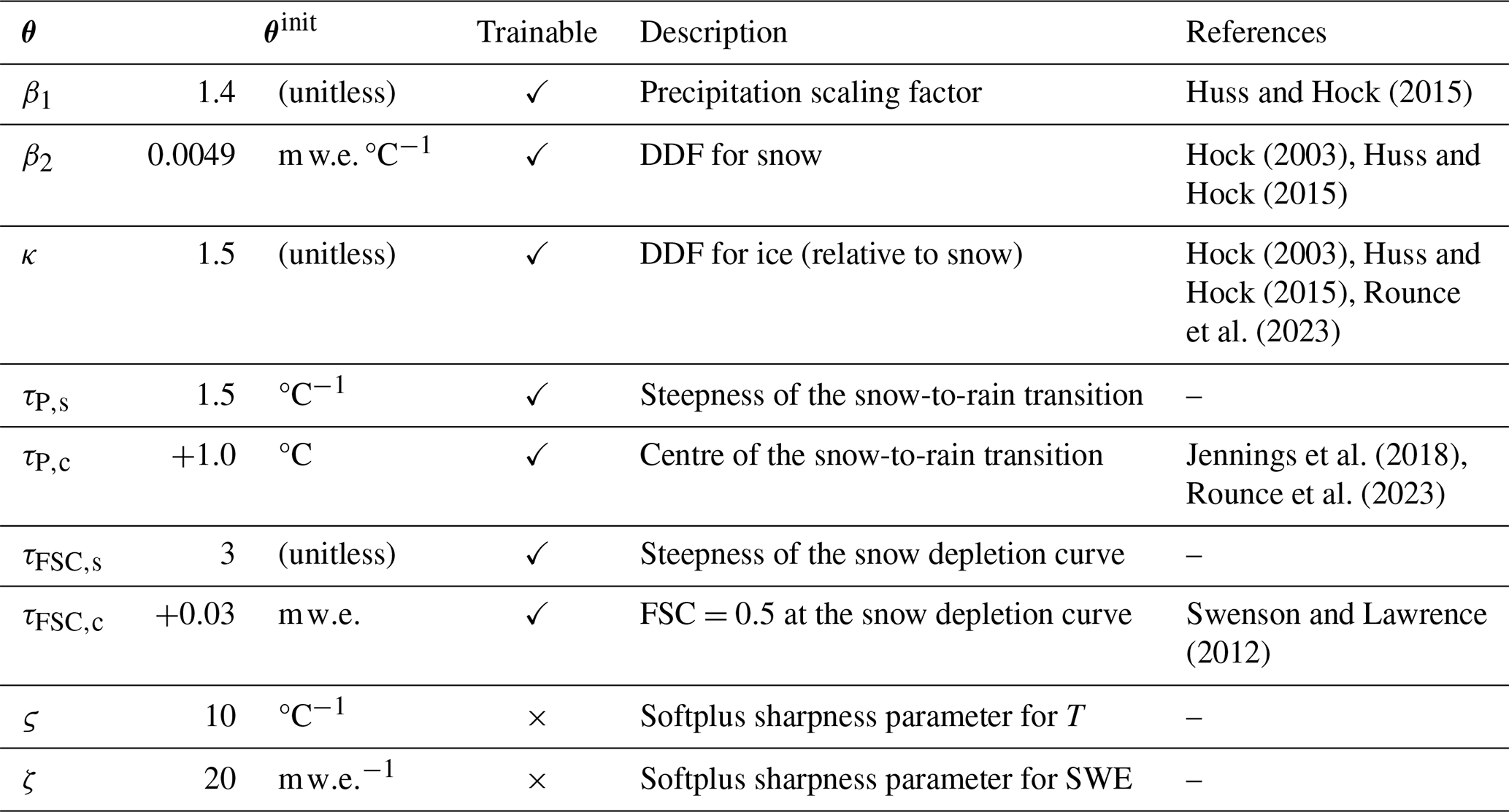

Table 1 TI model parameters and their initial values.

The parameters of the model are constrained as follows:

$$\begin{array}{}\text{(11)}& {\mathit{\beta }}_{\mathrm{1}},{\mathit{\beta }}_{\mathrm{2}},\mathit{\kappa }-\mathrm{1},{\mathit{\tau }}_{P,\text{s}},{\mathit{\tau }}_{\mathrm{FSC},\mathrm{s}},{\mathit{\tau }}_{\mathrm{FSC},\mathrm{c}},\mathit{\varsigma },\mathit{\zeta }>\mathrm{0},\end{array}$$

where $\mathit{\theta }={\left[{\mathit{\beta }}_{\mathrm{1}},{\mathit{\beta }}_{\mathrm{2}},\mathit{\kappa },{\mathit{\tau }}_{P,\mathrm{s}},{\mathit{\tau }}_{P,\mathrm{c}},{\mathit{\tau }}_{\mathrm{FSC},\mathrm{s}},{\mathit{\tau }}_{\mathrm{FSC},\mathrm{c}},\mathit{\varsigma },\mathit{\zeta }\right]}^{\top }$ are the TI model parameters. The initial values of the parameters are chosen based on the literature priors by averaging reported values and to remain physically consistent, those are summarised in Table 1. Our formulation is consistent with the classic two-DDF TI model, while remaining differentiable everywhere. It allows for calibration with gradient descent and its variants or even with higher-order methods, mitigating the suboptimality of grid search often employed for TI model calibration (Huss and Hock, 2015; Zekollari et al., 2024; van der Meer et al., 2025). An explicit comparison with a conventionally calibrated non-smooth TI formulation is provided in Appendix C, showing nearly identical performance.

4.2 Purely data-driven GRU baseline

As a purely data-driven baseline with no physical inductive bias, we employ a simple one-layer gated recurrent unit (GRU) model (Model B). The GRU is a variant of a recurrent neural network that introduces gating mechanisms to mitigate vanishing gradient issues and to better capture long-term dependencies through internal memory management. The GRU is defined as (Cho et al., 2014):

$$\begin{array}{}\text{(12)}& \begin{array}{rl}{\displaystyle }& {\displaystyle }{\mathit{z}}_{ijd}=\mathit{\sigma }\left({\mathbf{W}}_z{\mathit{x}}_{ijd}+{\mathbf{U}}_z{\mathit{h}}_{ijd-\mathrm{1}}+{\mathit{b}}_z\right),\\ {\displaystyle }& {\displaystyle }{\mathit{r}}_{ijd}=\mathit{\sigma }\left({\mathbf{W}}_r{\mathit{x}}_{ijd}+{\mathbf{U}}_r{\mathit{h}}_{ijd-\mathrm{1}}+{\mathit{b}}_r\right),\\ {\displaystyle }& {\displaystyle }{\widehat{\mathit{h}}}_{ijd}=\tanh \left({\mathbf{W}}_h{\mathit{x}}_{ijd}+{\mathbf{U}}_h\left[{\mathit{r}}_{ijd}\odot {\mathit{h}}_{ijd-\mathrm{1}}\right]+{\mathit{b}}_h\right),\\ {\displaystyle }& {\displaystyle }{\mathit{h}}_{ijd}=(\mathrm{1}-{\mathit{z}}_{ijd})\odot {\mathit{h}}_{ijd-\mathrm{1}}+{\mathit{z}}_{ijd}\odot {\widehat{\mathit{h}}}_{ijd},\end{array}\end{array}$$

where ${\mathit{x}}_{ijd}={\left[T_{ijd},P_{ijd}\right]}^{\top }$ is the input vector, z is the update gate, r is the reset gate, $\widehat{\mathit{h}}$ is the candidate hidden state, h is the hidden state, ⊙ stands for the Hadamard product, and ${\mathbf{W}}_z,{\mathbf{W}}_r,{\mathbf{W}}_h,{\mathbf{U}}_z,{\mathbf{U}}_r,{\mathbf{U}}_h,{\mathit{b}}_z,{\mathit{b}}_r,{\mathit{b}}_h$ are trainable parameters. In the implementation, the GRU receives normalised inputs, corresponding to the temperature and precipitation values divided by their maximum-absolute values. Similar to the TI model, we initialise h₀ as a trainable vector at the year y−5 and run the simulation for five consecutive years to obtain the starting conditions for the period of interest. Finally, the SMB output is computed as a linear projection of the hidden state vector:

$$\begin{array}{}\text{(13)}& {\widehat{\text{SMB}}}_{ijd}={\mathbf{W}}_{\mathrm{SMB}}{\mathit{h}}_{ijd}+b_{\mathrm{SMB}},\end{array}$$

where W_SMB and b_SMB are also trainable parameters.

We chose the GRU as the baseline due to its topological similarities with our TI formulation. Both models treat each grid cell independently, apply non-linear transformations to daily temperature and precipitation inputs, operate sequentially forward in time and maintain a single internal memory state (the SWE in the TI model and the hidden state h in the GRU) through a single computational unit. Unlike the TI model, the GRU imposes no physical inductive bias and instead relies on a flexible, high-capacity parameterisation. We fix the hidden state dimension to 16, resulting in 961 trainable parameters compared to 7 in the TI model. This contrast in model capacity enables a controlled assessment of whether a physics-informed structure provides advantages over a purely data-driven model in capturing SMB variability.

4.3 GlaUnTI

As the third comparative model, we propose GLAcier-UNiversal Temperature Index model (GlaUnTI), a modification of the autodiff-friendly TI model that attaches multiplicative correctors to the precipitation sensitivity and DDF terms:

$$\begin{array}{}\text{(14)}& {\widehat{\text{SMB}}}_{ijd}={\mathit{\beta }}_{\mathrm{1}}{e}^{{\mathrm{\Delta }}_{ijy}^{\left(\mathrm{1}\right)}}{P}_{ijd}^{\mathrm{solid}}-{\mathit{\beta }}_{\mathrm{2}}{e}^{{\mathrm{\Delta }}_{ijy}^{\left(\mathrm{2}\right)}}\left(T_{ijd}^{+,\mathrm{snow}}+\mathit{\kappa }{e}^{{\mathrm{\Delta }}_{ijy}^{\left(\mathrm{3}\right)}}{T}_{ijd}^{+,\mathrm{ice}}\right),\end{array}$$

and additive correctors to the rain-to-snow transition centre and the ERA5-Land temperature bias:

$$\begin{array}{}\text{(15)}& \begin{array}{rl}{\displaystyle }& {\displaystyle }{P}_{ijd}^{\mathrm{solid}}=P_{ijd}\cdot \mathit{\sigma }\left({\mathit{\tau }}_{P,\text{s}}\left[{\mathit{\tau }}_{P,\text{c}}+{\mathrm{\Delta }}_{ijy}^{\left(\mathrm{4}\right)}-T_{ijd}\right]\right),\\ {\displaystyle }& {\displaystyle }{T}_{ijd}^{+}={\text{softplus}}_{\mathit{\varsigma }}\left(T_{ijd}+{\mathrm{\Delta }}_{ijy}^{\left(\mathrm{5}\right)}\right),\end{array}\end{array}$$

where ${\mathbf{\Delta }}_y^{\left(\mathrm{1}\mathrm{\dots }\mathrm{5}\right)}$ are matrices of glacier- and cell-specific corrections to the base TI parameters in year y, following the general ideas introduced by Reichstein et al. (2019), Bolibar et al. (2023) and Li et al. (2023). Consistent with Eq. (14), the multiplicative corrections are applied to the SWE as well:

$$\begin{array}{}\text{(16)}& \begin{array}{rl}{\text{SWE}}_{ijd}& ={\text{softplus}}_{\mathit{\zeta }}\left({\text{SWE}}_{ijd-\mathrm{1}}+{\mathit{\beta }}_{\mathrm{1}}{e}^{{\mathrm{\Delta }}_{ijy}^{\left(\mathrm{1}\right)}}{P}_{ijd}^{\mathrm{solid}}\right.\\ & \left.-{\mathit{\beta }}_{\mathrm{2}}{e}^{{\mathrm{\Delta }}_{ijy}^{\left(\mathrm{2}\right)}}{T}_{ijd}^{+,\mathrm{snow}}\right).\end{array}\end{array}$$

The architecture of the deep learning corrector is shown in Fig. 2. It consists of two branches. The first branch is a 2D-convolutional branch, and it processes spatially distributed predictors, which include an initial guess of the SMB from Model A (${\mathrm{SMB}}_{\mathrm{0}}=f(\mathbf{T},\mathbf{P})$, where f is Model A) and the sensitivities of the initial guess to small perturbations ($\mathbf{\Delta }{\mathrm{SMB}}_{\mathrm{0},\mathrm{\Delta }T}=f(\mathbf{T}+\mathrm{0.5}\mathit{°}\text{C},\mathbf{P})-{\mathrm{SMB}}_{\mathrm{0}}$, $\mathbf{\Delta }{\mathrm{SMB}}_{\mathrm{0},\mathrm{\Delta }P}=f(\mathbf{T},\mathbf{P}\cdot \mathrm{1.05})-{\mathrm{SMB}}_{\mathrm{0}}$) as well as the glacier outline mask (GM), surface elevation and its uncertainty (Z and Z_σ), and glacier facies predictors (GF) that include concatenated glacier facies masks (GF^⋆) and their confidence (s^⋆) introduced earlier. The inclusion of the initial guess and the sensitivities partially reflects the ideas from Jia et al. (2021) and Daw et al. (2021), where a data-driven model serves as a post-processing step for a physical model. The second branch is a 1D-convolutional branch that processes monthly aggregated time series of temperature (T_M) and precipitation (P_M) over the modelled year. The output of the second branch gets reprojected to match the shape of the output of the first branch, and both are fused with a simple summation. Two more convolutional layers are applied after that to enhance the fusion and the extraction of potentially useful hidden features from both branches jointly. Finally, bilinear resampling is applied to match the shape of the correctors with the shape of the glacier grid. This simple resampling is computationally efficient and provides a regularising effect due to the enforced smoothness of the outputs. Before entering the corrector, Z, Z_σ, T_M and P_M are divided by feature-specific maximum absolute values. SMB₀ is divided by 10 m w.e., corresponding to the typical magnitude order of measured point SMB. The perturbation-derived sensitivity fields, glacier masks and facies predictors are kept in their original ranges. Notably, Eq. (6) remains the main backbone of the GlaUnTI model, and the overparameterised corrector only influences its core parameters, hence, keeping the interpretability of the model high by design.

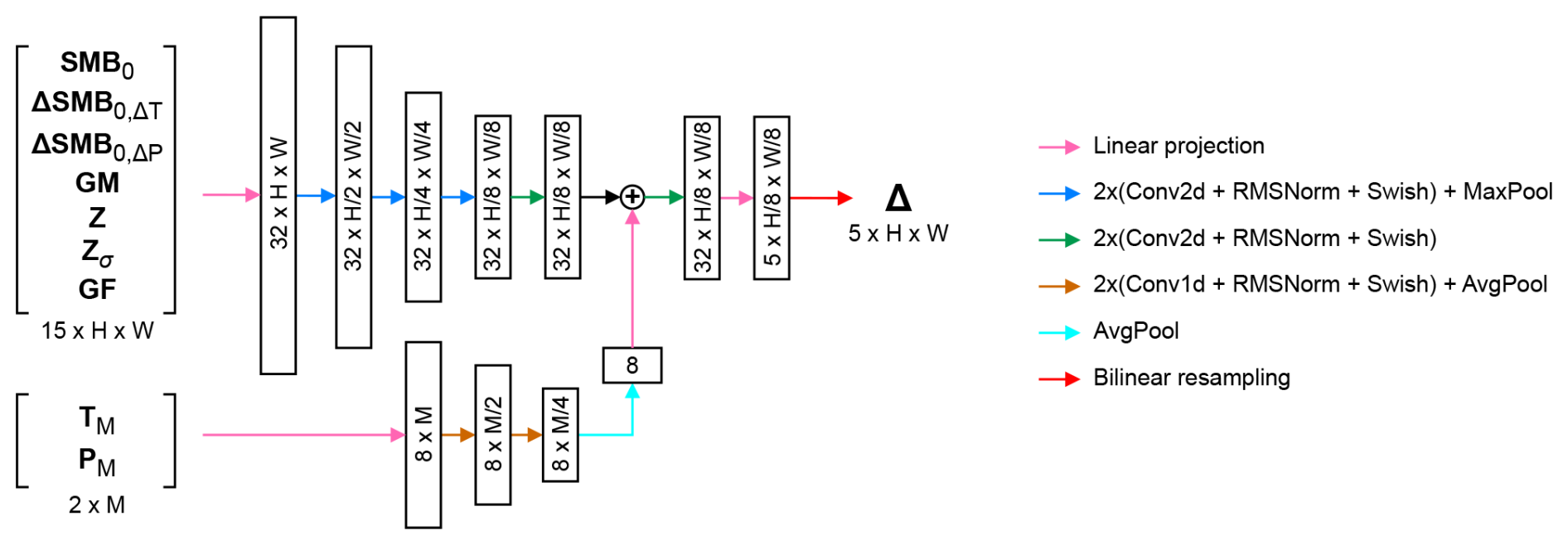
Figure 2 Deep learning corrector architecture. The shapes of tensors are denoted as $\text{channels}\times \text{height}\times \text{width}$ for the spatial branch and as channels×months for the temporal branch.

We distinguish two variants of the GlaUnTI model. The first one (Model C) is the model where all glacier facies predictors are replaced with a placeholder (−1 for each grid cell and facies channel), i.e. only the initial guess, glacier geometry and climate aggregates influence the correction terms. The second one (Model D) is where the actual values of GF are fed to the model where available, and the placeholder is used elsewhere, allowing for separate evaluation of the added value of glacier facies maps. Both variants have frozen TI parameters from trained Model A. The initial parameters of Model C are random, while those of Model D are initialised from trained Model C. Model C is trained to convergence before this transfer, and extended training without facies did not lead to further improvements in validation error. Hence, any performance gains in Model D cannot be explained by extended optimisation or a better starting point and are primarily associated with the inclusion of glacier facies predictors.

4.4 Model training and evaluation

We performed a stratified split of the dataset into six folds, balancing the number of glaciers, the number of glacier-wide SMB estimates, the number of point SMB measurements, the number of available glacier facies maps and the appearance of the five regions among the folds. The split was performed at the glacier level. For the stratification, each glacier was assigned to a stratum defined by its region and quantile-binned descriptors of data availability, namely, the number of point SMB measurements, the number of observation years and the number of available glacier facies maps. Glaciers were then assigned iteratively to the folds. At each step, the next glacier was placed into the fold with the lowest current number of glaciers from the same stratum. After that, we selected the first fold as the test one, the second one as the validation one and the rest as the training ones. Overall, the test subset contains 13 glaciers with 312/235/233 (annual/winter/summer) glacier-wide SMB reference values, 793/756/314 point measurements and 29 glacier facies maps. The validation subset includes 13 glaciers, 278/194/195 glacier-wide estimates, 2350/906/633 point measurement and 26 facies maps. The training subset consists of 52 glaciers, 1047/849/851 glacier-wide SMB estimates, 7340/13 759/2535 point SMB measurements and 108 facies maps. The split is shown in Fig. 1.

(Kingma and Ba, 2014)

Table 2 Models compared in this study.

All models, their training configurations and initial weight setups are summarised in Table 2. All four models are trained using daily temperature and precipitation inputs and the same loss definition. The training is done by minimising the following loss function on the glaciers from the training subset:

$$\begin{array}{}\text{(17)}& \begin{array}{rl}{\displaystyle }L& {\displaystyle }={\displaystyle \frac{\mathrm{1}}{n}}\sum _{ijy}{w}_{ijy}{\left({\widehat{\text{SMB}}}_{ijy}-{\text{SMB}}_{ijy}^{\mathrm{point}}\right)}^{\mathrm{2}}\\ {\displaystyle }& {\displaystyle }+{\mathit{\lambda }}_{\mathrm{1}}{\displaystyle \frac{\mathrm{1}}{m}}\sum _y{\left({\widehat{\text{SMB}}}_y^{\mathrm{total}}-{\text{SMB}}_y^{\mathrm{total}}\right)}^{\mathrm{2}}+\\ {\displaystyle }& {\displaystyle }+{\mathit{\lambda }}_{\mathrm{2}}{∥{\text{diag}}^{-\mathrm{1}}\left({\mathit{\theta }}^{\mathrm{init}}\right)\left(\mathit{\theta }-{\mathit{\theta }}^{\mathrm{init}}\right)∥}_{\mathrm{2}}^{\mathrm{2}}\\ {\displaystyle }& {\displaystyle }+{\mathit{\lambda }}_{\mathrm{3}}\sum _k{∥{\mathbf{\Delta }}^{\left(k\right)}∥}_{\mathrm{2}}^{\mathrm{2}}+\\ {\displaystyle }& {\displaystyle }+{\mathit{\lambda }}_{\mathrm{4}}\sum _k{\left({\mathbf{\Delta }}^{\left(k\right)}-\stackrel{\mathrm{‾}}{{\mathbf{\Delta }}^{\left(k\right)}}\right)}^{\mathrm{2}}+\\ {\displaystyle }& {\displaystyle }+{\mathit{\lambda }}_{\mathrm{5}}{\left({\mathbf{\Delta }}^{\left(\mathrm{3}\right)}-{\mathbf{\Delta }}^{\left(\mathrm{2}\right)}\right)}^{\mathrm{2}},\end{array}\end{array}$$

where ${\text{SMB}}_{ijy}^{\mathrm{point}}$ are measured annual/winter/summer point SMB mapped to the corresponding grid cell, ${\text{SMB}}_y^{\mathrm{total}}$ are glacier-wide SMB estimates, n and m are the number of point measurements and glacier-wide estimates, respectively, w_ijy are the point-specific SMB weights that reduces the influence of the point measurements with the timings misaligned with the simulation period, λ₁ is the term that downweights the glacier-wide estimates as they are a result of extrapolation and we treat them rather like a spatial regulariser, λ_2…5 are additional regularisers, and $\stackrel{\mathrm{‾}}{\mathbf{\cdot }}$ stands for the spatial mean value. The regularisation terms λ_2…5 constrain the optimisation by anchoring the TI parameters to literature-based priors (λ₂), limiting the magnitude and spatial variability of the learned correction fields (λ₃, λ₄) and enforcing consistency between snow- and ice-melt corrections (λ₅). Numerically, λ₁=0.1 is chosen to be of the same order as the ratio of glacier-wide to point observation counts in the training set. We selected λ₂=0.1, λ₃=5, λ₄=20, λ₅=5 with grid search by running training for a couple of epochs so that the validation loss dynamics is optimal at the beginning; a more fine-grained tuning was not possible due to the high computational requirements. The simulation periods y are either annual (running from the beginning of a hydrological year to its end) or seasonal (running from the beginning of a hydrological year to the end of winter and from the end of winter to the end of the hydrological year) and are aligned with the dates assigned to the glacier-wide estimates of SMB in the dataset. These dates, however, are not always aligned with the point measurements as some field campaigns can occupy several days or there could be several independent campaigns. Hence, to account for this discrepancy and to avoid materialising daily SMB fields during training, which is prohibitive due to the memory constraints, we introduce the weights $w_{ijy}=\exp \left(-{\left[\frac{d_{\mathrm{1},y}-d_{\mathrm{1},ijy}^{\prime }}{\mathit{\eta }}\right]}^{\mathrm{2}}\right)\exp \left(-{\left[\frac{d_{\mathrm{2},y}-d_{\mathrm{2},ijy}^{\prime }}{\mathit{\eta }}\right]}^{\mathrm{2}}\right)$, where d_1,y and d_2,y are the dates defining the period of glacier-wide estimate, $d_{\mathrm{1},ijy}^{\prime }$ and $d_{\mathrm{2},ijy}^{\prime }$ are the dates of the point measurement, and η=6.36 d is the decay parameter estimated from the data, so that one Gaussian weight component computed from the 95th percentile of the date difference yields 0.05. Equation (17) is computed per glacier over the whole study period (1995–2024) from one continuous simulation, the corresponding gradients are summed up across the glaciers, and only one parameter update per epoch is applied.

The best model parameters are selected by tracking the loss values without regularisers (i.e. λ_2…5=0) on the validation glaciers and saving only the best-performing models. The best trained models were then evaluated on a spatially independent test subset of 13 glaciers. The performance is reported in terms of Pearson's correlation coefficient, bias and RMSE:

$$\begin{array}{}\text{(18)}& \begin{array}{rl}{\displaystyle }& {\displaystyle }r={\displaystyle \frac{{\sum }_i\left({\widehat{y}}_i-\stackrel{\mathrm{‾}}{\widehat{y}}\right)\left(y_i-\stackrel{\mathrm{‾}}{y}\right)}{\sqrt{{\sum }_i{\left({\widehat{y}}_i-\stackrel{\mathrm{‾}}{\widehat{y}}\right)}^{\mathrm{2}}}\sqrt{{\sum }_i{\left(y_i-\stackrel{\mathrm{‾}}{y}\right)}^{\mathrm{2}}}}},\\ {\displaystyle }& {\displaystyle }\text{bias}={\displaystyle \frac{\mathrm{1}}{n}}\sum _i\left({\widehat{y}}_i-y_i\right),\\ {\displaystyle }& {\displaystyle }\text{RMSE}=\sqrt{{\displaystyle \frac{\mathrm{1}}{n}}\sum _i{\left({\widehat{y}}_i-y_i\right)}^{\mathrm{2}}},\end{array}\end{array}$$

where y_i is the reference SMB value, ${\widehat{y}}_i$ is the model output, and $\stackrel{\mathrm{‾}}{\mathbf{\cdot }}$ stands for the mean value. Evaluation is done at both point and glacier-wide level, and we report both annual and seasonal performance where possible. The exact dates for point measurements are used to report the test performance, without the weighting logic (i.e. no w_ijy) used for training and validation, as dense daily SMB time series are produced in this case.

All models were trained and evaluated on a cloud server equipped with an NVIDIA RTX A6000 GPU, a 128-core CPU (2.5 GHz) and 1 TB of RAM. In this setup, training the basic TI model (Model A) and the GRU baseline (Model B) required approximately 12 and 36 h, respectively, while training the GlaUnTI models (Models C and D) required approximately 48 h. Once trained, forward simulation of SMB for a single glacier over the full 30-year study period is computationally inexpensive and takes on the order of seconds. All models were implemented in Python (v3.13.5) using JAX (v0.6.0) for automatic differentiation and just-in-time compilation.

5 Results

This section evaluates the predictive performance of the four SMB models on a spatially independent test set of 13 glaciers not used during training or validation. Performance is assessed at both point-level SMB measurements obtained from the glaciological method and glacier-wide SMB estimates. We report correlation, bias and RMSE for annual and seasonal SMB, first aggregated across all test glaciers and subsequently resolved at the individual-glacier level to assess robustness and transferability in more detail. The results are presented in Figs. 3–5 and summarised quantitatively below.

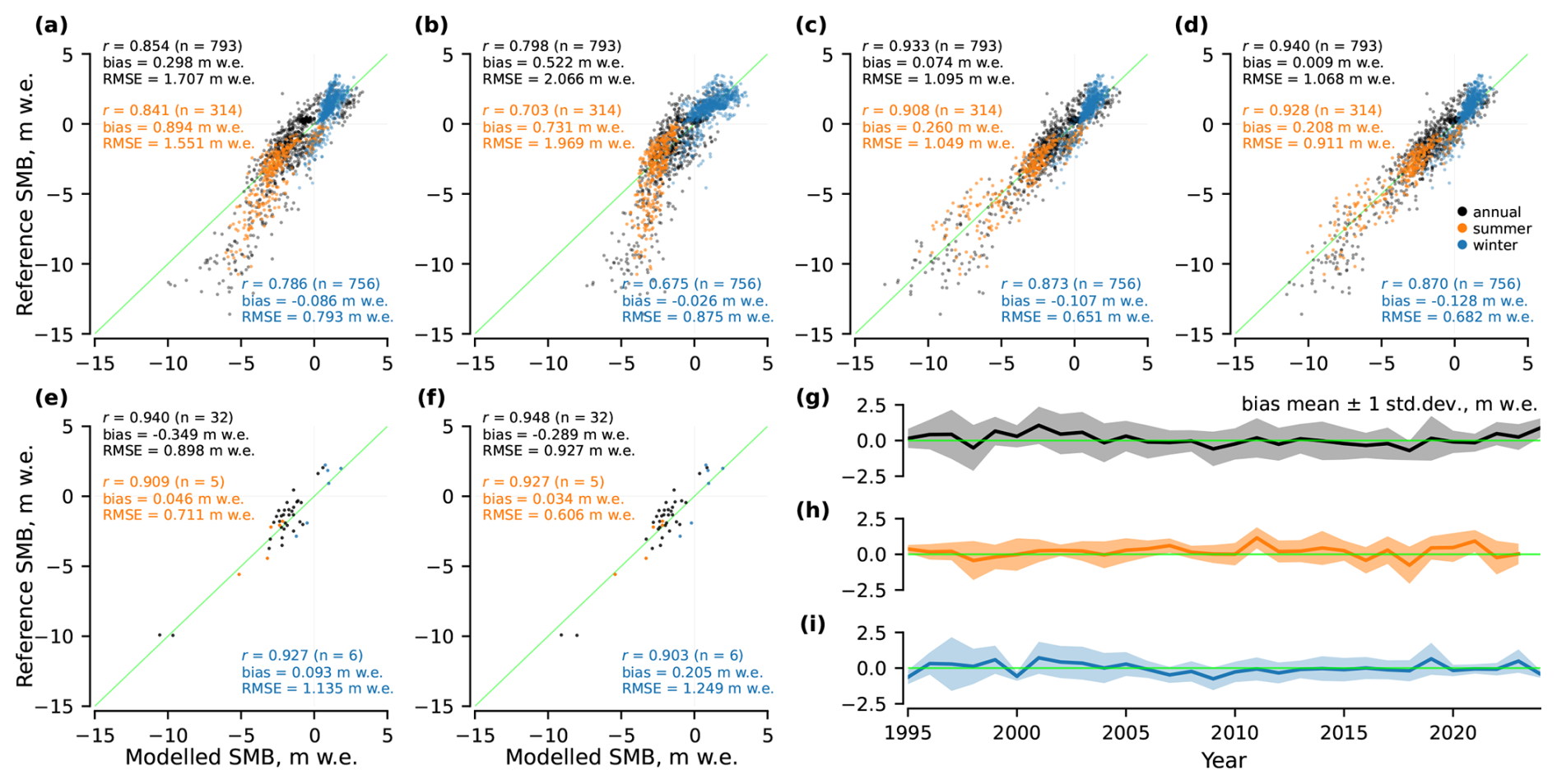
Figure 3 Point-level performance of the SMB models on the test glaciers: for (a) Model A, (b) Model B, (c) Model C, (d) Model D, (e) Model C for glaciers and years where glacier facies maps are available, (f) Model D for glaciers and years where glacier facies maps are available, and (g–i) bias mean and spread per year for Model D.

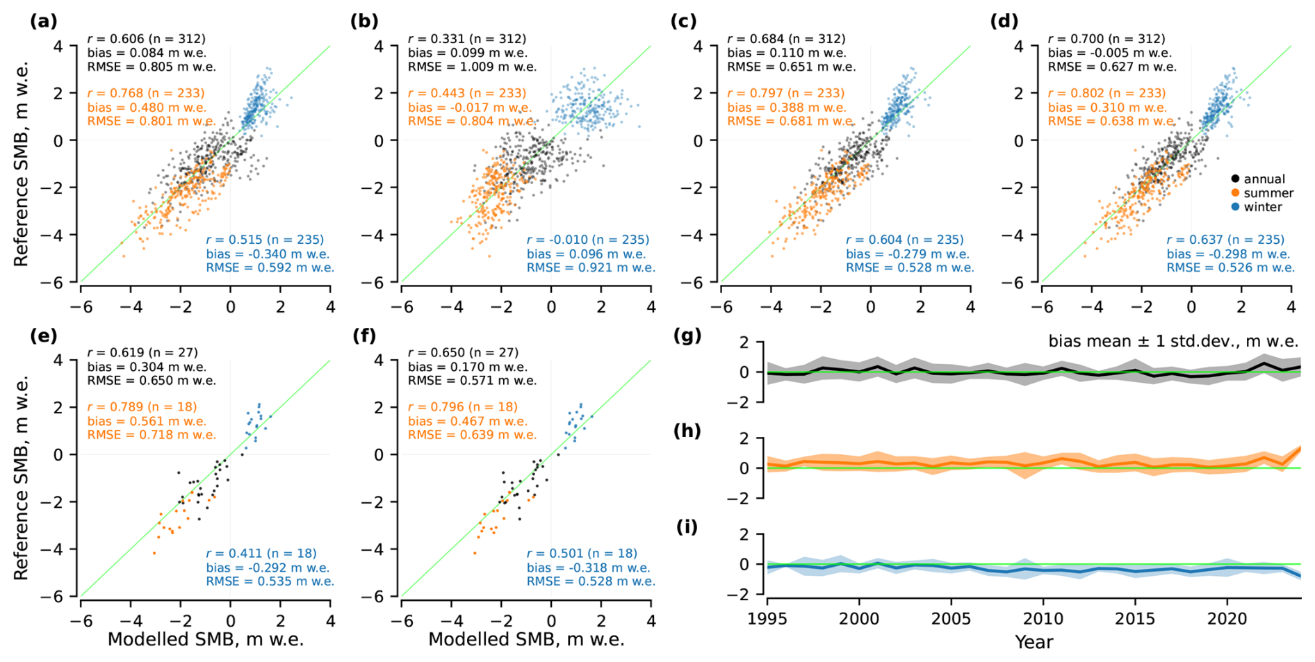
Figure 4 Glacier-wide performance of the SMB models on the test glaciers: for (a) Model A, (b) Model B, (c) Model C, (d) Model D, (e) Model C for glaciers and years where glacier facies maps are available, (f) Model D for glaciers and years where glacier facies maps are available, and (g–i) bias mean and spread per year for Model D.

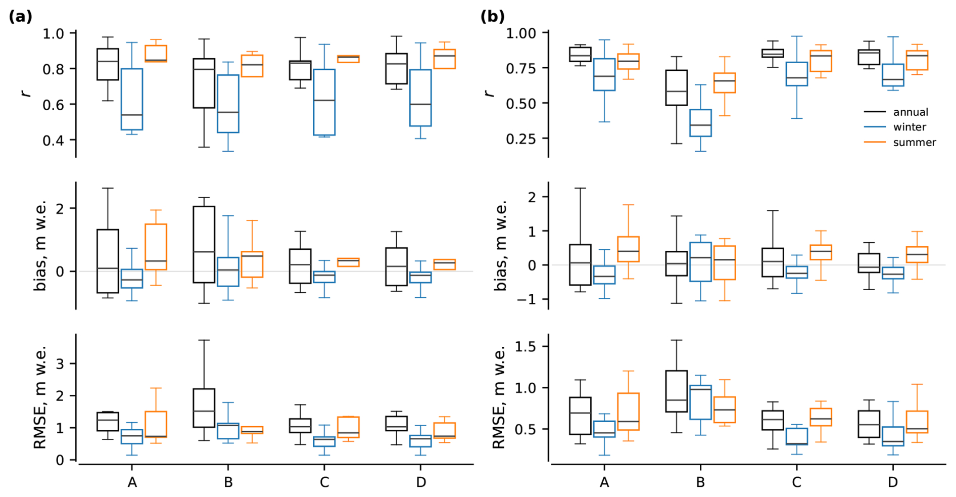
Figure 5 Per-glacier performance of the SMB models on the test glaciers: for (a) point measurements and for (b) glacier-wide estimates. A, B, C and D correspond to the different models (see Table 2).

5.1 Point-level performance

Figure 3 summarises point-level performance of the models. For each observation, the modelled SMB is aggregated over the exact measurement period reported in the dataset, and compared to the corresponding reference value. Model A achieves an annual correlation of r=0.854 (n=793), with $\text{RMSE}=\mathrm{1.707}\mathrm{m}\mathrm{w}.\mathrm{e}.$ and mean $\text{bias}=+\mathrm{0.298}\mathrm{m}\mathrm{w}.\mathrm{e}.$. Model B shows a lower correlation (r=0.798) and a higher RMSE (2.066 m w.e.), with $\text{bias}=+\mathrm{0.522}\mathrm{m}\mathrm{w}.\mathrm{e}.$ Notably, both Models A and B demonstrate a noticeable tail of underestimated melt as the reference SMB values decrease. The GlaUnTI models improve substantially over both baselines. Model C reaches r=0.933, $\text{RMSE}=\mathrm{1.095}\mathrm{m}\mathrm{w}.\mathrm{e}.$ and $\text{bias}=+\mathrm{0.074}\mathrm{m}\mathrm{w}.\mathrm{e}.$ Model D yields r=0.940, $\text{RMSE}=\mathrm{1.068}\mathrm{m}\mathrm{w}.\mathrm{e}.$ and $\text{bias}=+\mathrm{0.009}\mathrm{m}\mathrm{w}.\mathrm{e}.$ Relative to Model A, Model C and Model D reduce the annual point-level RMSE by approximately 0.61 (35.9 %) and 0.64 m w.e. (37.4 %), respectively. Summer and winter performance generally follows the same ranking across models, with Models C and D consistently reducing the RMSE and absolute bias relative to Models A and B, with the only exception of the winter bias that remains the lowest for Model B. Figure 3g–i indicate that Model D maintains a near-zero mean bias over time. For the subset of glaciers and years where glacier facies maps are available (n=32 annual point measurements), Models C and D retain high annual correlations (r=0.940 and 0.948), yet without convincing improvements from including glacier facies maps, especially given the limited set of seasonal point measurements.

5.2 Glacier-wide performance

At the glacier-wide scale (Fig. 4), Model A achieves an annual correlation of r=0.606 (n=312), with $\text{RMSE}=\mathrm{0.805}\mathrm{m}\mathrm{w}.\mathrm{e}.$ and $\text{bias}=\mathrm{0.084}\mathrm{m}\mathrm{w}.\mathrm{e}.$ Model B exhibits substantially weaker annual correlation (r=0.331) and a higher RMSE (1.009 m w.e.), while maintaining near-zero mean biases. Models C and D improve glacier-wide performance relative to both baselines. Model C achieves r=0.684 with $\text{RMSE}=\mathrm{0.651}\mathrm{m}\mathrm{w}.\mathrm{e}.$ and $\text{bias}=+\mathrm{0.110}\mathrm{m}\mathrm{w}.\mathrm{e}.$ Model D yields the best overall glacier-wide performance with r=0.700, $\text{RMSE}=\mathrm{0.627}\mathrm{m}\mathrm{w}.\mathrm{e}.$ and $\text{bias}=-\mathrm{0.005}\mathrm{m}\mathrm{w}.\mathrm{e}.$ Relative to Model A, Model D reduces the annual glacier-wide RMSE by approximately 0.18 m w.e. (22.1 %). Model D also maintains a near-zero mean bias over time, yet with a higher tendency to underestimate both glacier melt in summer and accumulation in winter (Fig. 4g–i). Seasonal glacier-wide performance shows consistent improvements for Models C and D relative to Models A and B across the summer and winter subsets. For the facies-available subset (n=27 annual estimates), Model D further reduces the RMSE (from 0.718 to 0.639 m w.e.) and absolute bias (from 0.561 to 0.467 m w.e.) relative to Model C for summer and, hence, annual estimates.

5.3 Per-glacier performance

Resolving performance by glacier, Fig. 5 shows per-glacier performance across the 13 spatially independent test glaciers in terms of distributions of correlation, bias and RMSE evaluated separately for point-level measurements and glacier-wide SMB estimates. For both evaluation scales, Models C and D consistently reduce the per-glacier RMSE relative to Models A and B annually and in winter. In particular, the median per-glacier RMSEs are lower and the interquartile ranges are narrower for Models C and D, indicating that the improvements observed in the aggregate metrics are robust across the test glaciers. Model B exhibits the largest inter-glacier variability, with wide spreads in all metrics. Seasonal differences are evident at the glacier scale, with winter performance showing lower correlations and higher variability than summer performance for all models; however, Models C and D generally outperform Models A and B in both seasons. Overall, the GlaUnTI models (C and D) generalise robustly to spatially independent glaciers and their performance gains are systematic.

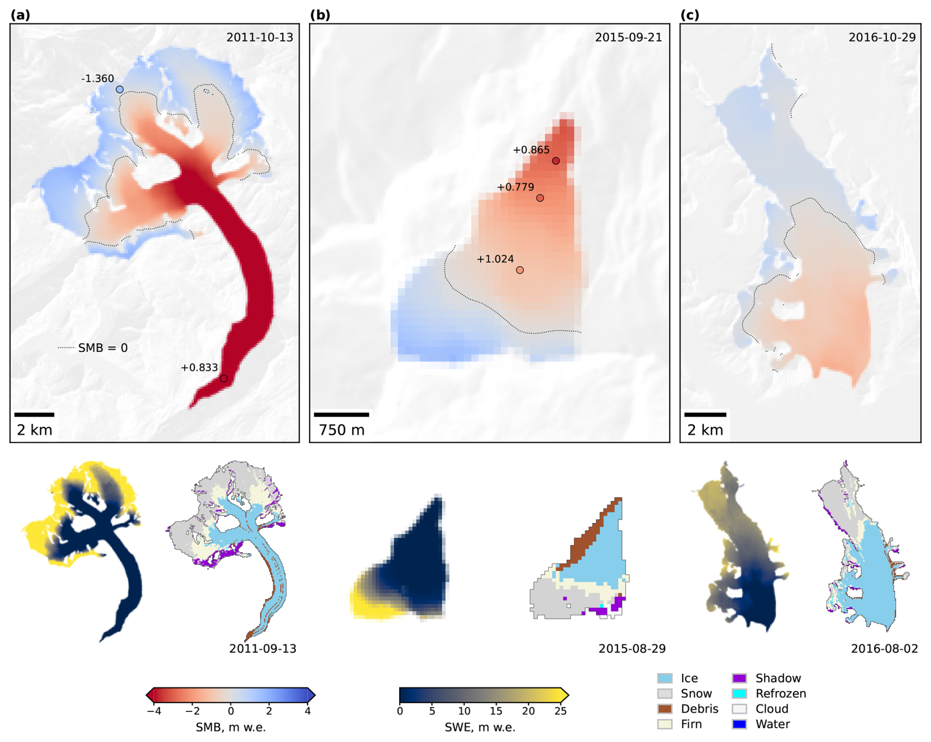
Figure 6 Annual SMB maps produced by Model D for: (a) Grosser Aletsch in 2011, (b) Schwarzberg in 2015 and (c) Hansbreen in 2016. Each panel shows the predicted annual SMB field (top), SWE (bottom left) and a glacier facies map derived from optical satellite imagery acquired near the end of the ablation season (bottom right). Dates in the SMB panels indicate the end date of the annual SMB measurement period, while dates in the facies maps indicate the acquisition dates of the corresponding satellite images. Point markers show available in-situ SMB measurements. Labels next to the points show point-level prediction errors in m w.e., calculated as predicted SMB minus measured SMB.

5.4 Qualitative assessment of modelled SMB

Figure 6 provides qualitative examples of the spatial structure of annual SMB fields predicted by Model D for three glaciers from the test subset. The modelled SMB patterns are spatially coherent and follow the expected elevation-dependent structure, with negative SMB over lower ablation areas and positive SMB over upper accumulation areas. The modelled equilibrium line positions (indicated by the SMB=0 contour) are also broadly consistent with the glacier facies maps acquired near the end of the ablation season: snow tends to occur above or near the modelled equilibrium line. The accompanying SWE fields provide an additional consistency check. The largest end-of-period snow storage is generally located in the upper accumulation areas and decreases towards the ablation zones. The point-level errors shown in the SMB panels indicate that the spatially distributed fields are locally consistent with available in-situ measurements, although individual deviations remain. An important nuance is that the SMB/SWE states and facies maps are not always perfectly co-temporal. This temporal mismatch is particularly visible for Hansbreen (Fig. 6c), where the facies map precedes the SMB end date by almost three months, meaning that subsequent late-season accumulation can affect the SMB and SWE states without being represented in the facies map.

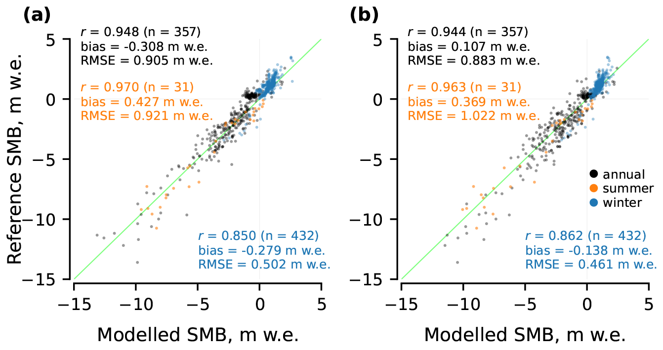
Figure 7 Point-level performance over the independent 2019–2024 evaluation period of (a) Model A finetuned separately for each test glacier and (b) the original Model D without glacier-specific finetuning.

5.5 Comparison with glacier-specific TI calibration

To separate the benefit of spatial transferability from the performance achievable through local calibration, we additionally finetuned Model A independently for each of the 13 test glaciers. For each glacier, all available point measurements and glacier-wide SMB estimates from 1995–2012 were used for finetuning, while observations from 2013–2018 were used as the validation subset. The period 2019–2024 was kept completely independent and used only for performance evaluation. Model D was not finetuned in this experiment and was used directly with the parameters obtained from the original spatial training, i.e. without using any observations from the test glaciers. This setup deliberately favours Model A, since its parameters can adapt to earlier observations from the same glacier on which it is subsequently evaluated. Nevertheless, Model D remains highly competitive over the independent 2019–2024 period (Fig. 7). For annual point SMB, the per-glacier finetuned Model A reaches r=0.948, $\text{bias}=-\mathrm{0.308}\mathrm{m}\mathrm{w}.\mathrm{e}.$ and $\text{RMSE}=\mathrm{0.905}\mathrm{m}\mathrm{w}.\mathrm{e}.$, compared with r=0.944, $\text{bias}=+\mathrm{0.107}\mathrm{m}\mathrm{w}.\mathrm{e}.$ and $\text{RMSE}=\mathrm{0.883}\mathrm{m}\mathrm{w}.\mathrm{e}.$ for Model D. The same pattern is observed seasonally. Model D has a lower absolute bias in both winter and summer and comparable RMSEs, with slightly lower winter and slightly higher summer RMSE. Hence, GlaUnTI approaches the performance of glacier-specific TI calibration while retaining transferability to glaciers without local calibration data.

6 Discussion

Overall, our results show that combining a TI backbone with a learnable, spatially distributed correction improves the ability of the model to generalise to spatially independent glaciers. Across the held-out test set spanning five heterogeneous European regions, the hybrid models reduce the annual point-scale RMSE from 1.707 m w.e. (Model A) to 1.068 m w.e. (Model D, 37.4 %) and annual glacier-wide RMSE from 0.805 to 0.627 m w.e. (22.1 %), while maintaining near-zero mean bias at both scales. This reduction is consistent with the core hypothesis that a physically structured TI formulation imposes a strong inductive bias, and that the neural corrector is then forced to spend its capacity primarily on persistent, glacier-specific or climate-specific residual errors rather than relearning the full accumulation and ablation mappings from scratch.

A quantitative comparison with recent SMB modelling studies highlights both the competitiveness of our results and the importance of the evaluation scope. In the French Alps, a deep learning SMB model reaches a glacier-wide RMSE of 0.51 m w.e. under a leave-one-glacier-out validation (Bolibar et al., 2020), which is comparable to our glacier-wide RMSE of 0.627 m w.e. obtained from a spatially independent suite of glaciers. In Switzerland, an XGBoost-based approach achieves a point-scale RMSE of 0.604 m w.e. (versus 0.687 m w.e. for a TI baseline), representing a 13.7 % improvement (van der Meer et al., 2025). These results, however, reflect a single-country domain with relatively homogeneous conditions. In the European Alps, a machine learning model reports an annual point RMSE of 1.071 m w.e. (Anilkumar et al., 2023), close to our 1.068 m w.e. despite our use of spatially independent glaciers for evaluation. In Norway, an XGBoost model attains an annual point RMSE of 1.00 m w.e. (0.35–1.37 m w.e. per glacier) and a glacier-wide RMSE of 0.54 m w.e. (Sjursen et al., 2025). Our corresponding values of 1.068 m w.e. (0.469–1.51 m w.e. per glacier) and 0.627 m w.e. fall within the same performance range. In the same study and under the same experimental protocol (Sjursen et al., 2025), established glacier evolution models – OGGM (Maussion et al., 2019), GloGEM (Huss and Hock, 2015) and PyGEM (Rounce et al., 2023) – yield annual point RMSEs of 0.9–1.1 m w.e., indicating that GlaUnTI performs on par with process-based approaches. For Svalbard, CryoGrid simulations achieve substantially lower point-scale errors of 0.33 m w.e. (Schmidt et al., 2023), though these results lack a spatial hold-out evaluation and benefit from higher-quality regional forcing, limiting comparability. Hence, absolute RMSE values must be interpreted jointly with domain heterogeneity, forcing quality and evaluation protocols. Our key result is the consistent improvement from Models A and B to Models C and D across glaciers and seasons.

The poor transfer performance of the purely data-driven GRU baseline (Model B), particularly at the glacier-wide scale (annual r=0.331), highlights the need for a strong structural prior in geoscientific applications with sparse and diverse observational networks. A model with flexible state dynamics can fit local idiosyncrasies in the training glaciers yet fails to generalise to new geometries and climate regimes. In contrast, the TI backbone acts as a structural regulariser. It enforces physically interpretable monotonic responses (temperature-driven melt and precipitation-driven accumulation), preserves a meaningful internal state and implicitly constrains extrapolation under domain shifts. The neural corrector of GlaUnTI then learns where and when those simplified assumptions fail systematically, e.g. persistent precipitation underestimation, elevation-dependent temperature biases, spatial patterns tied to shading and facies-related albedo and water retention effects, while remaining anchored to the physics-informed backbone.

The deviation tail visible for Models A and B at strongly negative SMB (underestimated melt at large ablation magnitudes) likely indicates missing or underrepresented processes. Plausible candidates are debris-enhanced melt or melt-albedo feedbacks not captured by the FSC proxy and not sufficiently expressed through temperature alone. Heterogeneous debris patterns and rugged terrain can produce localised high melt and strong representativeness errors at stake locations (Bisset et al., 2020). More broadly, during extreme melt seasons, enhanced and highly variable radiative forcing (and associated energy-balance shifts) can weaken the empirical link between air temperature and melt energy, challenging the “temperature as proxy” assumption (Litt et al., 2019). This interpretation is consistent with the observation that the hybrid corrector reduces the tail, while the predictive variance remains large (Fig. 3c, d). The corrector can compensate for systematic bias correlated with geometry and climate aggregates, but it cannot perfectly reconstruct process variability that is not identifiable from the chosen predictors. In a related way, point measurements themselves are not necessarily representative of the mean SMB of a 100 m grid cell resolution, particularly on large, topographically complex glaciers with strong microclimate gradients, wind redistribution and variable shading. The signal at the point scale mixes true process mismatch with unresolved subgrid variability and measurement representativeness. Another unresolved process is the absence of explicit advection of the SWE state. SWE is not transported with glacier flow, so coupling GlaUnTI to an ice dynamics model would be required for long-term projections or fast flowing glaciers. Similarly, uncertainty in surface elevation propagates into the temperature forcing, introducing additional errors at the point scale. This matters for both training and evaluation. The consistent improvement at the glacier-wide scale is therefore an important addition as aggregation averages out local noise, while Models C and D generally reduce the glacier-wide RMSE and increase correlations, indicating that GlaUnTI is not merely overfitting, but is also capturing coherent biases relevant to integrated mass balance.

Inclusion of the glacier facies maps into GlaUnTI yields moderate improvement in predicting summer glacier-wide SMB, yet the benefits for other target variables remain marginal. Facies products likely act as surrogate indicators for multiple unresolved processes simultaneously, including late-summer albedo history, firn retention capacity, debris cover, exposure of bare ice and the position of the snowline region, rather than facies being a causal driver per se. This is physically motivated because accumulation area extent and snowline position are closely linked to SMB (Rabatel et al., 2017, 2005; Hock et al., 2007; Drolon et al., 2016), while the facies classes also provide an observational proxy for surface-albedo contrasts between snow, firn, bare ice and debris. This reframes facies assimilation as a pragmatic way to inject remote sensing constraints on the state of the surface into an SMB model when direct energy balance forcing is unavailable. Moreover, because GlaUnTI propagates SWE through time, facies-based corrections can affect subsequent snow storage, melt partitioning and SMB beyond the exact years in which facies maps are available. This is consistent with the improvement of Model D over Model C in summer SMB even for years without directly available facies maps. The weak statistical separation between Models C and D here is also affected by the limited sample size (n=32 annual point measurements, n=27 annual glacier-wide estimates), limiting the ability to resolve modest but potentially real gains. Alternative remote sensing products might play similar roles, potentially with better temporal coverage than the end-of-summer facies maps, e.g., transient snowline altitude, bare-ice exposure duration or SAR melt intensity time series (as in Scher et al., 2021). Future extensions could also include more direct energy balance predictors, such as shortwave radiation, thermal infrared information and wind, but doing so would move the present TI model closer to a complete surface energy balance formulation.

Uncertainty in climate forcing explains a large portion of the modelled SMB error and remains a dominant constraint on SMB performance at large scales. The differentiable setup makes this limitation explicit. The aleatoric uncertainty propagation example (Appendix A3) illustrates how temporally correlated forcing discrepancies can generate uncertainty envelopes comparable to the observed model–reference mismatch for cumulative trajectories, emphasising that model performance should not be interpreted independently of the forcing uncertainties. This also has methodological implications. As models become more flexible (e.g., by introducing complex machine learning correctors), they can effectively compensate for biases in the climate forcing, improving agreement with observations. Without explicitly modelling forcing uncertainty, however, such corrections may combine the effects of forcing errors and structural model deficiencies in a way that complicates physical attribution. In practice, this suggests that future work should explicitly model and propagate uncertainties in climate forcing rather than treating them as unstructured residual noise, particularly when SMB is integrated into long-term projections where small daily errors accumulate.

The relationship between glaciological glacier-wide SMB estimates and geodetic mass change motivates a careful use of geodetic data to better constrain SMB models and to exploit the full range of available observations. Geodetic observations provide a valuable, spatially comprehensive constraint on glacier mass change, particularly where in situ SMB measurements are absent and, hence, represent a natural complement to the glaciological in situ data. Global geodetic products provide robust and internally consistent signals at regional to global scales, but their uncertainty at the individual glacier scale can be substantial for small glaciers and steep terrains (Hugonnet et al., 2021). In contrast, regional geodetic surveys, which often rely on higher resolution elevation models and region-specific processing, typically achieve lower uncertainties and are more suitable for constraining glacier-wide mass changes over decadal periods (Geissler et al., 2021; Van Tricht et al., 2023). Importantly, geodetic mass change is not strictly equivalent to surface mass balance. It integrates additional processes such as dynamic thinning, frontal ablation for calving glaciers and basal melt. Also, uncertainty in the effective density of elevation changes introduces a non-negligible source of error in geodetic mass balance estimates (Huss, 2013), further complicating their direct use as annual SMB targets. A promising path forward is therefore to use high-quality regional geodetic surveys as weak but informative constraints over sufficiently long time periods. For land-terminating glaciers, such constraints can act as upper bounds on cumulative SMB trajectories, helping to prevent long-term drift. This strategy would enable an SMB model to leverage as much useful information as possible from geodetic observations, while respecting the misalignment between the definitions of SMB and geodetic mass balance.

Finally, the autodiff-friendly formulation expands the role of the SMB models beyond the traditional task of predicting mass balances. Differentiability enables seamless coupling of surface processes with ice dynamics within a unified framework, in which gradients can propagate consistently from atmospheric forcing through SMB into ice flow and thickness change. This directly facilitates integration with differentiable ice-flow frameworks such as the Instructed Glacier Model (IGM; Jouvet et al., 2022) and the Open global glacier model + DIfferential equation Neural Networks (ODINN.jl; Bolibar et al., 2023), opening a way towards joint SMB–dynamics modelling systems in which surface and dynamic processes are treated as interacting components rather than as sequential modules. Such coupled frameworks are particularly valuable for investigating short-term or sustained atmospheric forcing anomalies that influence ice dynamics, including changes in basal sliding, velocity variability and surge behaviour, as documented in observational and modelling studies linking climate forcing to dynamic glacier response (Burgess et al., 2013; Flowers et al., 2016). Such a framework would allow these interactions to be explored in a consistent and computationally efficient manner. Beyond methodological advances, this capability has direct relevance for policy applications. The inverse modelling example (Appendix A1) demonstrates how gradient-based optimisation can be used to infer effective forcing perturbations required to stabilise glacier-wide SMB over a target period. Because the full modelling chain is GPU-driven, such analyses can, in principle, be efficiently scaled to regional or continental scales, enabling systematic evaluation of climate sensitivities and stabilisation thresholds. These results provide a basis for translating climate forcing scenarios into regionally aggregated targets, with potential relevance for assessments reported in IPCC frameworks and for the formulation of climate change mitigation strategies explicitly focused on glacier preservation.

7 Conclusions

In this study, we introduced GlaUnTI, a hybrid SMB modelling framework that couples an autodiff-friendly TI backbone with a lightweight convolutional corrector that learns glacier- and cell-specific adjustments to the key TI parameters while preserving the physical model structure. Across a spatially independent pan-European test set spanning 1995–2024, several contrasting glacier regions and 13 glaciers, GlaUnTI reduced annual point SMB error by 37.4 % and annual glacier-wide error by 22.1 % relative to the baseline TI model, while maintaining near-zero bias and improving robustness across individual glaciers and seasons. These results support the central premise that a physics-informed backbone provides a strong inductive bias for out-of-sample generalisation, while the learned corrector primarily expends capacity on systematic residual errors associated with regional forcing biases, topographic effects and simplified melt and accumulation assumptions. The proposed framework is intended to be extensible toward additional observational constraints. A wide class of remote sensing proxies, such as albedo products, transient snowline altitude or SAR melt indicators, can provide information on processes that are poorly represented by temperature and precipitation alone and may therefore help correct systematic structural error. End-to-end differentiability enables efficient calibration, transfer learning, inverse optimisation, attribution with respect to atmospheric forcing and first-order propagation of forcing uncertainty (Appendix A), and it provides a natural route to incorporate geodetic mass change products as weak, multi-annual constraints that reduce long-term drift of predicted SMB. Finally, the same design facilitates coupling to differentiable ice flow frameworks, enabling consistent sensitivity analyses from climate forcing through SMB into ice dynamics and supporting scenario- and mitigation-relevant questions such as estimating stabilisation thresholds in terms of effective forcing perturbations on regional scales.

Appendix A: Illustrative applications of differentiability

In this appendix, we demonstrate additional benefits of the autodiff-friendly TI formulation. Specifically, we illustrate three case studies enabled by differentiability of the full TI forward model – (i) gradient-based inverse modelling, (ii) model explainability through input attribution and (iii) first-order propagation of forcing-driven aleatoric uncertainty. In all examples, we take a glacier from the test subset and finetune Model A on all available point measurements and glacier-wide estimates from 1995–2012, using 2013–2018 as the validation subset for early stopping. Model performance is reported for a temporally independent test period (2019–2024) in order to avoid inflation of results due to temporal leakage. We deliberately use the lowest-complexity model due to the limited amount of single-glacier training data and the methodological focus of these demonstrations rather than the pursuit of the best predictive accuracy. Jointly, these three examples illustrate how differentiability transforms the TI model from a purely predictive tool into a flexible framework for scientific analysis and interpretation with modest programming efforts and computational requirements.

A1 Inverse modelling

We first demonstrate the use of the autodiff-friendly TI formulation for gradient-based inverse modelling by estimating an effective temperature perturbation required to balance the annual glacier-wide SMB over a recent period. The example illustrates how sensitivities of cumulative SMB with respect to climate forcing can be exploited to adjust forcing trajectories to meet the constraints imposed on the modelled SMB.

Similarly to the differentiation w.r.t. model parameters during calibration, it is possible to differentiate the model w.r.t. its inputs or latent perturbations attached to them and solve a constrained optimisation problem for the forcing. In this particular case, we shift the temperature time series by a scalar offset ΔT_2015…2024 in 2015–2024 and then minimise the following objective:

$$\begin{array}{}\text{(A1)}& L={\left({\displaystyle \frac{\mathrm{1}}{\mathrm{5}}}\sum _{y=\mathrm{2020}}^{\mathrm{2024}}{\widehat{\text{SMB}}}_y^{\mathrm{total}}\right)}^{\mathrm{2}}+\mathit{ϵ}\mathrm{\Delta }{T}_{\mathrm{2015}\mathrm{\dots }\mathrm{2024}}^{\mathrm{2}},\end{array}$$

where $\mathit{ϵ}=\mathrm{1}{e}^{-\mathrm{4}}$ is a small regularisation term that slightly improves convergence. Minimising L w.r.t. ΔT_2015…2024 then answers the question: “What temperature change during 2015–2024 is required to bring the modelled glacier-wide SMB into equilibrium with the mean climate state over 2020–2024?” This setup should be interpreted as a deliberately reduced inverse experiment rather than a complete climate-change scenario. In a more complete setting, the joint distribution of temperature and precipitation would need to be modified, including changes in precipitation amount and frequency.

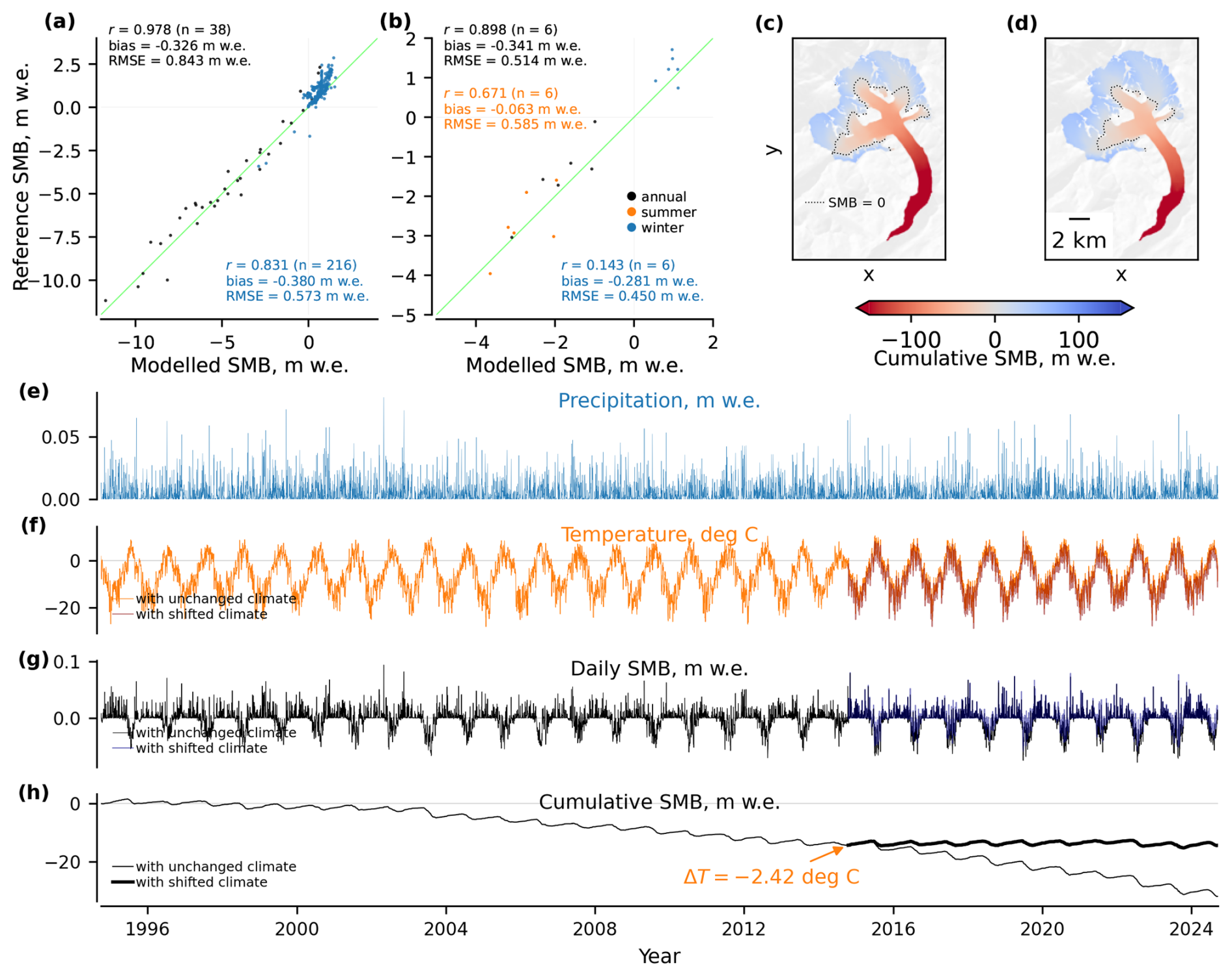
Figure A1 Inverse modelling case study for Grosser Aletsch: (a) point-level performance in 2019–2024 of the finetuned model, (b) glacier-wide performance, (c) cumulative SMB over 1995–2024 with unchanged ERA5-Land forcing, (d) cumulative SMB with shifted temperature time series, (e) precipitation time series, (f) temperature time series, (g) predicted daily SMB, and (h) cumulative glacier-wide SMB trajectory for original ERA5-Land forcing and with the forcing adjusted after inverse modelling.

We apply this procedure to Grosser Aletsch in the Swiss Alps and hold the glacier geometry fixed over the inversion period (i.e., the model is run with static outlines and elevation) to isolate the effect of forcing perturbations. Figure A1 summarises both the model performance and the inversion outcome. Over the temporally independent evaluation period, the finetuned model exhibits good glacier-wide annual performance (Fig. A1b), while the point-scale errors are larger (Fig. A1a), as expected given unresolved local processes and representativeness limitations for a large glacier with several variably oriented tributaries. The optimisation yields an effective temperature offset of $\mathrm{\Delta }{T}_{\mathrm{2015}\mathrm{\dots }\mathrm{2024}}=-\mathrm{2.42}$ °C (Fig. A1h), which increases the modelled glacier-wide cumulative SMB over the recent decade and brings the average annual glacier-wide SMB in 2020–2024 to zero by construction. This inferred ΔT_2015…2024 should be interpreted as an effective forcing perturbation within the TI modelling system, i.e. it compensates for both climatic forcing discrepancies and residual model biases remaining after finetuning (including the reported negative annual glacier-wide bias of $-\mathrm{0.343}\mathrm{m}\mathrm{w}.\mathrm{e}.$), yet the former dominates.

A2 Model explainability

We next illustrate how the autodiff-friendly TI formulation enables attribution of glacier-wide SMB to specific components of the climate forcing using integrated gradients (Sundararajan et al., 2017). This analysis provides insight into the relative contributions of temperature and precipitation anomalies at different times of the year to interannual variations in glacier-wide SMB.

Integrated gradients are an explainable artificial intelligence method that is commonly used to evaluate the influence of particular inputs on the outputs in deep learning models. In practice, it works with any differentiable non-linear model, as in our case. Given an input trajectory X_y (e.g., the forcing sequence for year y) and a baseline trajectory X^′, integrated gradients attribute the difference in the model output between X_y and X^′ to individual input dimensions by integrating input gradients along the straight line path connecting the baseline to the input (Sundararajan et al., 2017):

$$\begin{array}{}\text{(A2)}& \mathrm{\text{IG}}\left({\mathbf{X}}_y\right)=\left({\mathbf{X}}_y-{\mathbf{X}}^{\prime }\right)\odot \underset{\mathit{\alpha }=\mathrm{0}}{\overset{\mathrm{1}}{\int }}{\mathbf{\nabla }}_{{\mathbf{X}}_y}f\left({\mathbf{X}}^{\prime }+\mathit{\alpha }\left[{\mathbf{X}}_y-{\mathbf{X}}^{\prime }\right]\right)\mathrm{d}\mathit{\alpha }.\end{array}$$

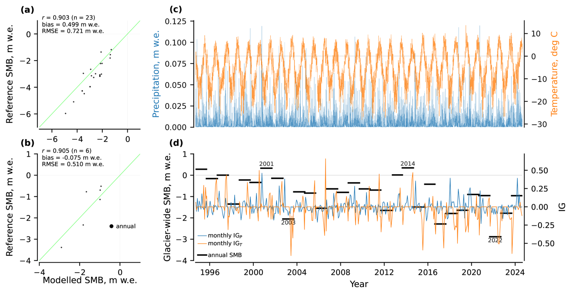
Figure A2 Model explainability case study for Schwarzberg: (a) point-level performance in 2019–2024 of the finetuned model, (b) glacier-wide performance, (c) ERA5-Land forcing, and (d) annual glacier-wide SMB with monthly aggregated values of integrated gradients for precipitation and temperature overlayed. The positive (negative) values of integrated gradients indicate a positive (negative) contribution to SMB as compared to the baseline climate over 1995–2024.

We apply this method to Schwarzberg in the Swiss Alps. As baseline forcing, we use the monthly climatology over 1995–2024, and we compute integrated gradients for each year relative to this baseline. Figure A2 summarises the evaluation and attribution results. Over the temporally independent evaluation period, the model shows adequate annual glacier-wide performance (Fig. A2b), supporting interpretation of annual attribution patterns at the glacier-wide scale. Point-scale errors are larger (Fig. A2a), similar to the previous case. The integrated-gradient time series in Fig. A2d provides an interpretable decomposition of annual glacier-wide SMB anomalies into temperature- and precipitation-associated contributions relative to the baseline. Positive (negative) integrated-gradient values indicate a positive (negative) contribution to SMB compared to baseline climate, enabling identification of years in which anomalously warm conditions (temperature contributions) or anomalous accumulation (precipitation contributions) dominate the SMB anomaly. The integrated-gradient attribution highlights physically consistent responses of glacier-wide SMB to anomalous climate conditions in individual years, yet does so in a formal and objective manner. For instance, Fig. A2d shows that the strongly negative SMB anomaly in 2003 is dominated by a large negative temperature contribution, reflecting the exceptionally warm summer conditions that affected large parts of central Europe during that year. Similarly, the pronounced negative SMB in 2022 is primarily associated with sustained positive temperature anomalies extending over a long melt season, consistent with widespread reports of extreme summer warmth and enhanced ablation. In contrast, the positive SMB anomaly in 2001 is associated with a strong positive precipitation contribution, indicating above-average snowfall during the accumulation season. The year 2014 exhibits a positive SMB anomaly despite near-average precipitation, which is instead attributed to a cooler-than-average summer and reduced melt.

A3 First-order aleatoric uncertainty quantification

Finally, we demonstrate first-order propagation of climate forcing uncertainty through the TI model using automatic differentiation to quantify forcing-driven aleatoric uncertainty in cumulative glacier-wide SMB. The example highlights how temporally correlated errors in temperature and precipitation translate into aleatoric uncertainty envelopes for long-term mass balance trajectories.

A common first-order approximation for uncertainty propagation through a general differentiable model f is obtained through linearisation around the mean input (also known as the delta method):

$$\begin{array}{}\text{(A3)}& \begin{array}{rl}{\displaystyle }& {\displaystyle }{\mathrm{\Sigma }}_y=\mathbb{E}\left[\left(Y-{\mathit{\mu }}_y\right){\left(Y-{\mathit{\mu }}_y\right)}^{\top }\right],\\ {\displaystyle }& {\displaystyle }Y-{\mathit{\mu }}_y\approx f\left({\mathit{\mu }}_x\right)+J\left(X-{\mathit{\mu }}_x\right)-{\mathit{\mu }}_y\approx J\left(X-{\mathit{\mu }}_x\right),\\ {\displaystyle }& {\displaystyle }{\mathrm{\Sigma }}_y\approx \mathbb{E}\left[J\left(X-{\mathit{\mu }}_x\right){\left(X-{\mathit{\mu }}_x\right)}^{\top }{J}^{\top }\right]=J{\mathrm{\Sigma }}_x{J}^{\top },\end{array}\end{array}$$

where $J={\left.\frac{\partial f}{\partial X}\right|}_{X={\mathit{\mu }}_x}$, X and Y stand for input and output variables of f, and Σ_x and Σ_y are covariance matrices of X and Y.

In our case, we represent forcing uncertainty through a latent perturbation vector z:

$$\begin{array}{}\text{(A4)}& z\in {\mathbb{R}}^{\mathrm{2}K},z\sim \mathcal{N}\left(\mathrm{0},\mathbf{I}\right),\end{array}$$

and generate perturbed physical forcing fields as a deterministic transformation:

$$\begin{array}{}\text{(A5)}& X=g\left(z\right),\end{array}$$

where g applies the following transformations to the temperature (T) and precipitation (P) time series:

$$\begin{array}{}\text{(A6)}& g_t^T\left(z\right)=T_t+{\mathit{\sigma }}_T{z}_{b\left(t\right)}^T,g_t^P\left(z\right)=P_t\exp \left({\mathit{\sigma }}_{\log P}{z}_{b\left(t\right)}^P\right),\end{array}$$

with $b\left(t\right)\in \left\{\mathrm{0},\mathrm{\dots },K-\mathrm{1}\right\}$ assigning each day t to one of K temporal blocks, σ_T denoting the standard deviation of additive temperature errors, and σ_log P standing for the standard deviation of multiplicative precipitation errors in logarithmic space. The perturbations are assumed to be spatially coherent over the glacier domain, consistent with the spatial resolution of the ERA5-Land data for small glaciers. The full SMB cumulative trajectory is therefore:

$$\begin{array}{}\text{(A7)}& y\left(z\right)=f\left(g\left(z\right)\right)\in {\mathbb{R}}^L,z=\left[z^T,z^P\right],\end{array}$$

where f is the model yielding a cumulative SMB trajectory, L is the number of daily time steps in the trajectory.

Finally, the variance of the cumulative glacier-wide SMB is evaluated as:

$$\begin{array}{}\text{(A8)}& \mathrm{Var}\left[y_t\right]={\left({\mathrm{\Sigma }}_y\right)}_{tt}\approx \sum _{j=\mathrm{1}}^{\mathrm{2}K}{\left(J_z\right)}_{tj}^{\mathrm{2}},J_z={\left.{\displaystyle \frac{\partial y}{\partial z}}\right|}_{z=\mathrm{0}}\end{array}$$

In practice, this summation is evaluated using Jacobian-vector products (J_ze_j) in chunks without explicit construction of Σ_y or J_z due to the memory constraints for large L.

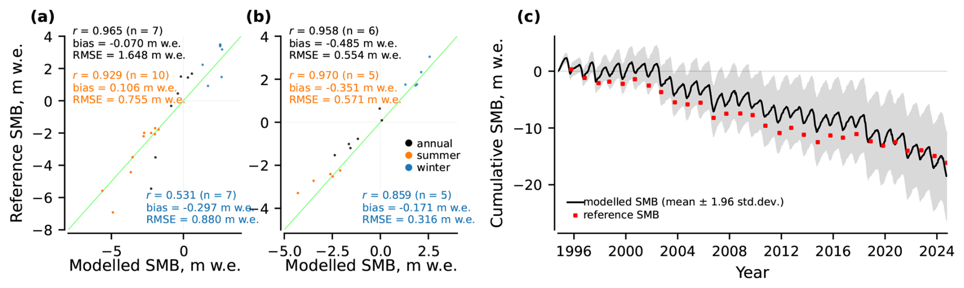
Figure A3 Aleatoric uncertainty propagation case study for Rembesdalskaaka: (a) point-level performance in 2019–2024 of the finetuned model, (b) glacier-wide performance, and (c) cumulative glacier-wide SMB trajectory. The shaded envelope represents forcing-driven aleatoric uncertainty obtained by propagating ERA5-Land forcing discrepancies through the SMB model using first-order automatic differentiation.

We demonstrate this procedure for Rembesdalskaaka in Southern Norway. Figure A3 reports both forward-model performance and the resulting uncertainty envelope. While point-scale SMB exhibits larger errors due to unresolved local processes (Fig. A3a), the model performs substantially better for glacier-wide SMB (Fig. A3b), which is the relevant scale for the cumulative trajectory and this uncertainty analysis. We calibrate σ_T, σ_log P and the block structure K by analysing residuals between ERA5-Land and E-OBS (Cornes et al., 2018) temperature and precipitation over the glacier domain and their temporal autocorrelation. For this case study, the selected block configuration corresponds to weekly blocks (approximately 7 d per block) and is chosen based on temperature as the more conservative estimate. For the presented example, we obtain σ_T=1.59 and σ_log P=0.96, which are also consistent with similar estimates reported in other studies (Prein and Gobiet, 2017; Delhasse et al., 2020; Dalla Torre et al., 2024). The shaded envelope in Fig. A3c represents forcing-driven aleatoric uncertainty only and does not include observational uncertainty in reference SMB values, parameter uncertainty or structural model error. Nevertheless, the magnitude of the forcing-driven envelope is comparable to the observed model–reference mismatch in this case study (all annual reference points lie within the displayed 1.96σ envelope), indicating that uncertainty in climate forcing is generally a major contributor to SMB uncertainty in modelling studies.

Appendix B: Data-driven imputation of elevation voids

This appendix describes the data-driven imputation procedure used to fill missing values in the surface elevation time series (Hugonnet et al., 2021). The objective is to infer plausible elevation values in the original voids, as evaluated on withheld data with known elevations, while preserving realistic uncertainty estimates.

First, we constructed a library of 223 void patterns by extracting all connected void regions from the full elevation dataset. For each glacier, synthetic voids were generated by randomly selecting void patterns from this library, applying random rotations and translations, and placing them on non-void elevation cells while ensuring that they did not overlap with any existing voids. These synthetic voids temporarily hide cells with known elevations and serve as validation masks, i.e. the imputation accuracy can be evaluated in these areas. Synthetic void patterns were added iteratively until the total glacier-wide void fraction matched the maximum void coverage observed across all glaciers (4.69 %), providing a realistic validation scenario. This procedure was repeated five times for each glacier, providing five independent synthetic void realisations that are treated as validation sets.

Next, we calibrated regression void-filling models that predict elevation from the following predictors – horizontal coordinates of each grid cell, Copernicus GLO-30 DEM features (elevation, slope and aspect) and acquisition year of the elevation raster being imputed. For each synthetic void realisation, the models were calibrated per glacier using non-void cells and evaluated against the withheld synthetic voids. Non-linear relationships between the predictors (x) and the Hugonnet et al. (2021) data were modelled using random Fourier features (sklearn.kernel_approximation.RBFSampler; Rahimi and Recht, 2008) followed by Bayesian ridge regression, which also provides posterior uncertainty estimates. A predictor vector x was first mapped into a D-dimensional random Fourier feature space:

$$\begin{array}{}\text{(B1)}& \mathit{\varphi }\left(\mathit{x}\right)=\sqrt{{\displaystyle \frac{\mathrm{2}}{D}}}\left[\cos \left({\mathit{w}}_{\mathrm{1}}^{\top }\mathit{x}+b_{\mathrm{1}}\right),\mathrm{\dots },\cos \left({\mathit{w}}_D^{\top }\mathit{x}+b_D\right)\right],\end{array}$$

where ${\mathit{w}}_i\sim \mathcal{N}\left(\mathrm{0},\mathrm{2}\mathit{\gamma }\mathbf{I}\right)$, $b_i\sim \mathcal{U}\left[\mathrm{0},\mathrm{2}\mathit{\pi }\right]$, and D, γ are hyperparameters. In this feature space, the imputed elevation $\widehat{y}$ was modelled as:

$$\begin{array}{}\text{(B2)}& \widehat{y}\left(\mathit{x}\right)=\mathit{\varphi }(\mathit{x}{)}^{\top }\mathit{\beta }+{\mathit{\beta }}_{\mathrm{0}},\end{array}$$

where β and β₀ are learnable parameters estimated via the procedure implemented in sklearn.linear_model.BayesianRidge. These methods were chosen as a computationally efficient approximation to kernel regression, avoiding poor scalability for the large number of grid cells and repeated fits required here.

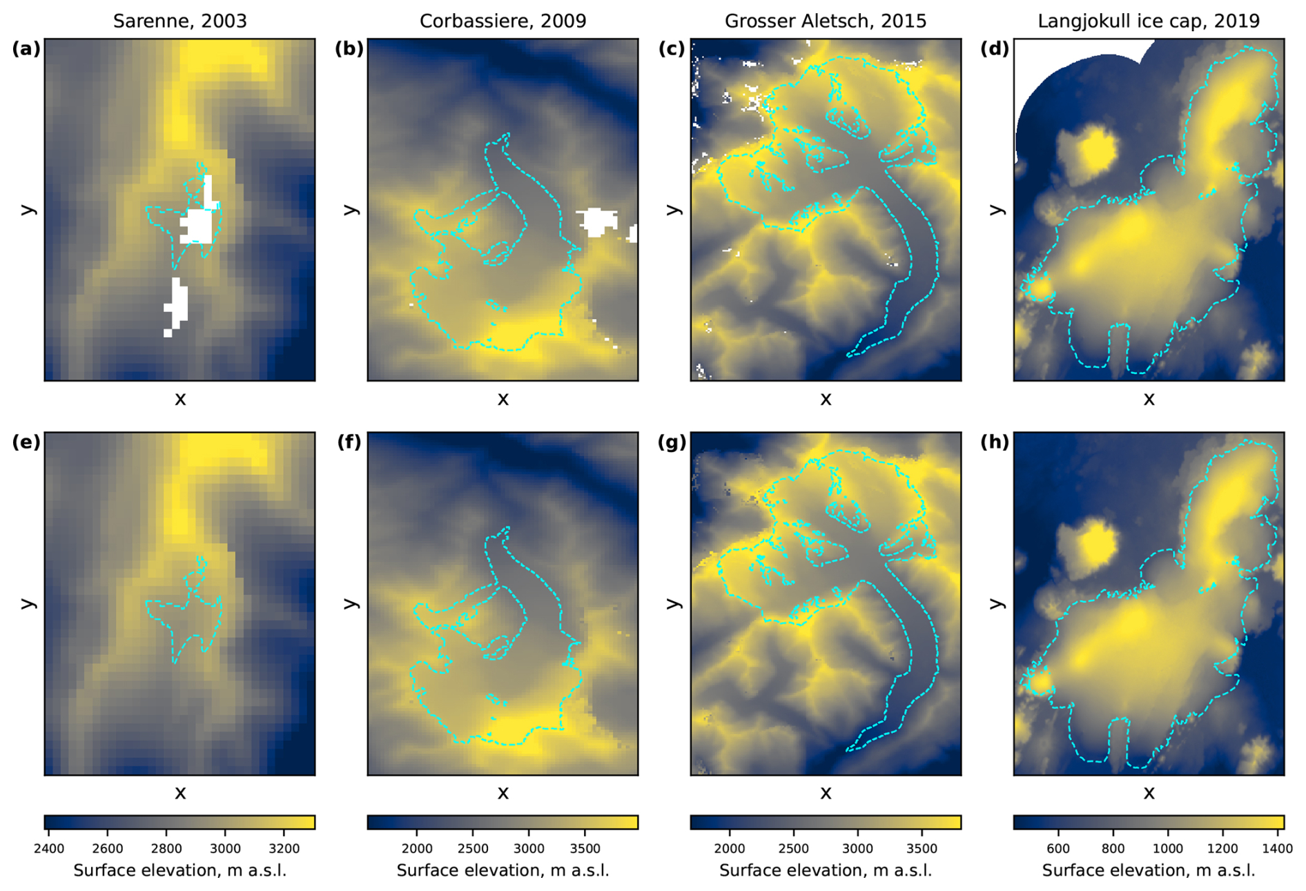
Figure B1 Results of the elevation void imputation: (a–d) original elevation rasters from Hugonnet et al. (2021), and (e–h) the same data with imputed voids. Void regions are shown in white. Glacier outlines are taken from RGI7.0 (RGI Consortium, 2023).

The model hyperparameters (γ, D) were optimised using Bayesian optimisation by minimising the mean RMSE between the modelled and the Hugonnet et al. (2021) data across the five synthetic void realisations and all glaciers. Across all glaciers, this procedure yielded a mean imputation RMSE of 14.8 m, comparable to the reported uncertainties of global elevation products (Podgórski et al., 2019; Chen et al., 2022). It is also consistent with the mean pixel-wise uncertainty of 10 m assumed in the Hugonnet et al. (2021) data themselves. After finding the optimal hyperparameters, the regression models were retrained using all available non-void elevation data (i.e. without synthetic voids) and subsequently applied to impute the original voids. Examples of the imputed elevation data are provided in Fig. B1. The posterior standard deviation from Bayesian ridge regression was retained as an estimate of elevation 1σ uncertainty associated with the imputed values.

Appendix C: Comparison with a classical non-smooth TI formulation

To verify that the smooth approximations introduced to make Model A compatible with automatic differentiation do not degrade the performance of the TI backbone, we implemented an otherwise comparable non-smooth TI formulation. The daily SMB is given by:

$$\begin{array}{}\text{(C1)}& {\displaystyle }{\widehat{\text{SMB}}}_{ijd}={\mathit{\beta }}_{\mathrm{1}}{P}_{ijd}^{\mathrm{solid}}-{\mathit{\beta }}_{\mathrm{2}}\left(T_{ijd}^{+,\text{snow}}+\mathit{\kappa }{T}_{ijd}^{+,\text{ice}}\right),\text{(C2)}& {\displaystyle }{P}_{ijd}^{\mathrm{solid}}=\left\{\begin{array}{ll}{P}_{ijd},& T_{ijd}\le T_{\mathrm{left}}\\ P_{ijd}\cdot {\displaystyle \frac{T_{\mathrm{left}}+L_{\mathrm{sr}}-T_{ijd}}{L_{\mathrm{sr}}}},& T_{\mathrm{left}}<T_{ijd}<T_{\mathrm{left}}+L_{\mathrm{sr}}\\ \mathrm{0},& T_{ijd}\ge T_{\mathrm{left}}+L_{\mathrm{sr}}\end{array}\right.,\text{(C3)}& {\displaystyle }{T}_{ijd}^{+,\text{snow}}={\text{FSC}}_{ijd}\cdot T_{ijd}^{+},\text{(C4)}& {\displaystyle }{T}_{ijd}^{+,\text{ice}}=\left(\mathrm{1}-{\text{FSC}}_{ijd}\right)\cdot T_{ijd}^{+},\text{(C5)}& {\displaystyle }{T}_{ijd}^{+}=max\left(\mathrm{0},T_{ijd}\right),\text{(C6)}& {\displaystyle }{\text{FSC}}_{ijd}=\left\{\begin{array}{ll}\mathrm{0},& {\text{SWE}}_{ijd-\mathrm{1}}<{\mathit{\tau }}_{\mathrm{FSC},\mathrm{c}}\\ \mathrm{1},& {\text{SWE}}_{ijd-\mathrm{1}}\ge {\mathit{\tau }}_{\mathrm{FSC},\mathrm{c}}\end{array}\right.,\text{(C7)}& {\displaystyle }{\mathrm{\text{SWE}}}_{ijd}=max\left(\mathrm{0},{\text{SWE}}_{ijd-\mathrm{1}}+{\mathit{\beta }}_{\mathrm{1}}{P}_{ijd}^{\mathrm{solid}}-{\mathit{\beta }}_{\mathrm{2}}{T}_{ijd}^{+,\text{snow}}\right),\end{array}$$

where ${\left[{\mathit{\beta }}_{\mathrm{1}},{\mathit{\beta }}_{\mathrm{2}},\mathit{\kappa },T_{\mathrm{left}},L_{\mathrm{sr}},{\mathit{\tau }}_{\mathrm{FSC},\mathrm{c}}\right]}^{\top }$ are the model parameters. T_left defines the temperature below which all precipitation is treated as solid, while L_sr defines the width of the linear snow-to-rain transition. The remaining parameters correspond directly to those of Model A. Compared with Eqs. (7)–(10), this formulation therefore replaces the smooth snow-to-rain transition, positive-temperature and SWE approximations, and fractional snow-cover transition by piecewise or threshold-based analogies.

We calibrated the classical formulation on the combined training and validation glacier subsets, while retaining the 13 test glaciers as a spatially independent evaluation set. Calibration was performed with an iterative grid search consisting of three refinement iterations. The first iteration explored broad parameter ranges, after which the ranges were progressively narrowed around the best-performing parameter set in the second and third iterations. Within each refinement, the accumulation-related parameters $\left({\mathit{\beta }}_{\mathrm{1}},T_{\mathrm{left}},L_{\mathrm{sr}}\right)$ and the ablation-related parameters $\left({\mathit{\beta }}_{\mathrm{2}},\mathit{\kappa },{\mathit{\tau }}_{\mathrm{FSC},\mathrm{c}}\right)$ were fitted in separate grid-search steps to keep the calibration computationally tractable. For a controlled comparison, we also recalibrated the autodiff-friendly formulation on the same combined training and validation glacier subsets. This calibration was run for 150 epochs, corresponding to approximately 36 h, i.e., a computational budget comparable to the classical grid search described above. The literature-prior regularisation was removed by setting λ₂=0, and the learning rate was increased to 0.1, allowing the gradient-based optimisation to explore the parameter space more freely. This was done because the classical calibration converged towards an effectively one-DDF solution, with ${\mathit{\tau }}_{\mathrm{FSC},\mathrm{c}}=\mathrm{0}$ and κ=1, which is far from the literature-based initial parameterisation used for Model A.

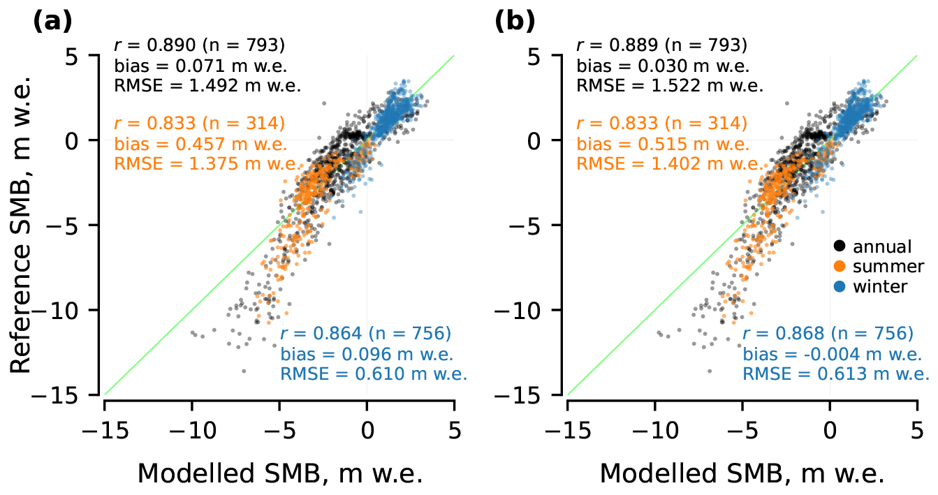
Figure C1 Point-level performance of (a) the classical non-smooth TI formulation and (b) the autodiff-friendly TI formulation on test glaciers.

In this setup, the two formulations show nearly identical point-level performance on the held-out test glaciers (Fig. C1). For annual SMB, the classical formulation reaches r=0.890, $\text{bias}=+\mathrm{0.071}\mathrm{m}\mathrm{w}.\mathrm{e}.$ and $\text{RMSE}=\mathrm{1.492}\mathrm{m}\mathrm{w}.\mathrm{e}.$, compared with r=0.889, $\text{bias}=+\mathrm{0.030}\mathrm{m}\mathrm{w}.\mathrm{e}.$ and $\text{RMSE}=\mathrm{1.522}\mathrm{m}\mathrm{w}.\mathrm{e}.$ for the autodiff-friendly formulation. The differences remain small seasonally. The corresponding winter RMSEs are 0.610 and $\mathrm{0.613}\mathrm{m}\mathrm{w}.\mathrm{e}.$, and the summer RMSEs are 1.375 and $\mathrm{1.402}\mathrm{m}\mathrm{w}.\mathrm{e}.$, respectively. Thus, replacing the classical threshold-based operations by the smooth approximations required for automatic differentiation does not materially affect the predictive performance of the TI backbone.