Introducing a new normalized cryospheric index (NCI) to categorize sub-watersheds on arid environments

This study examines sub-watersheds in the arid northern region of Chile (26°41^′–28°24^′ S), situated within the broader Copiapó watershed. The primary water source for this watershed originates from cryospheric landforms. The region exhibits pronounced physiographic and climatic diversity, with its northern sector situated within the South American Arid Diagonal (SAAD), where cryospheric features display greater spatial isolation. The aim of this study is to quantify the water volume contributed by distinct cryospheric landforms to regional watersheds. This study employs a classification methodology to categorize cryospheric landforms within sub-watersheds, integrating an inventory of cryospheric landforms, historical snow permanence derived from satellite imagery, published ice content and depth measurements (ERT and GPR). The Normalized Cryospheric Index (NCI) is calculated for varying hydrological conditions and provides a means to compare potential water volumes across sub-watersheds. The relative weight of ice and snow in the index is derived from the observed relationship between September snow cover and melt-season streamflow (ice weight w=0.43 on average, 0.27 in wet years and 0.62 in dry years). The analysis reveals significant spatial variability in cryospheric landforms and their strategic hydrological significance. Under average and low-precipitation conditions, the southern sub-watersheds of the Copiapó watershed show the greatest water storage potential. The Montosa River (NCI = 0.72 ± 0.12), Estero Come Caballos (NCI = 0.62 ± 0.23), Del Potro River (NCI = 0.61 ± 0.18), Manflas River (NCI = 0.59 ± 0.17), and Figueroa River (NCI = 0.50 ± 0.21) sub-watersheds have been identified as strategic priority areas within the region for sustaining surface runoff and safeguarding water availability. During high-snowfall periods, northern sub-watersheds in the Copiapo watershed, such as Estero Come Caballos, show elevated NCI values despite their limited cryospheric landforms. In contrast, the Montosa, Manflas, and Del Potro sub-watersheds contain the most extensive cryospheric landforms and rank among the top of the sub-watersheds with the highest NCI scores.

1 Introduction

Anthropogenic climate change impacts water availability, particularly in regions dependent on high-altitude water sources within mountain systems (Beniston and Stoffel, 2014; Beniston et al., 2018). Changes in the cryosphere that will occur within the next century include a change from solid to liquid precipitation, declining volumes of cryospheric landforms, snow lines moving to higher altitudes, and shorter snow seasons. With these changes, the predictions are that water resources in mountain areas will become increasingly scarce. In the arid zones of the Chilean Atacama Desert glaciers continue to shrink (Masiokas et al., 2020) and centennial reconstructions of rainfall patterns on the scale of hundreds of years, show a decline in rainfall in the Central Zone and the “Norte Chico” natural regions of Chile (Le Quesne et al., 2006; Minvielle and Garreaud, 2011; Morales et al., 2012; Bozkurt et al., 2017). In addition, the occurrence of mega droughts has intensified since 2010 (Garreaud et al., 2020).

Within this climatic context, the Copiapó River exhibits a mixed hydrological regime with very low discharges, typically ranging between ∼ 1.49 and 1.82 m³ s⁻¹ at the La Puerta gauging station, and strongly modulated by contributions from its main tributaries, the Manflas, Jorquera and Pulido Rivers, whose headwaters originate in high-altitude cryospheric environments. Long-term analyses indicate that mean annual flows rarely exceed 2 m³ s⁻¹ , and the watershed shows recurrent years of negative water balance, leading to progressive aquifer depletion (Suárez et al., 2014). These persistently low flows and the strong dependence on upstream snow and ice melt highlight the structural vulnerability of the runoff of the Copiapó River to changes in the cryosphere.

Because of the high altitude of the Andean cryosphere, precipitation is captured from air masses, predominantly in the form of snow. Generally, snow precipitation occurs during the winter (June-September), although the northern parts also receive snow during summer due to the Tropical Monsoon (i.e. Bolivian winter), which takes place from December to February (Valdivieso et al., 2022). In high-altitude Andean environments, snowfall does not directly translate into liquid runoff but may be preserved over different timescales through distinct cryospheric processes. Under favorable mass-balance conditions, repeated snow accumulation and firnification lead to the formation of debris-free glaciers. Where glacier ice becomes mantled by rockfall or talus material, debris-covered glaciers can develop, reducing ablation rates and enhancing ice preservation. In parallel, a significant fraction of snowfall infiltrates coarse debris slopes, where it refreezes and is preserved as ground ice within ice-rich permafrost landforms such as rock glaciers, protalus lobes, and gelifluction taluses. The melting of these cryospheric systems generates a sustained discharge of water, even during snow-free dry seasons. Given the extremely limited rainfall in the Andes, streamflow in the Copiapó River is strongly dependent on snowmelt and cryospheric water storage. (Masiokas et al., 2019). However, the contribution of cryospheric water storage to runoff varies substantially among cryospheric landforms types and occurs over contrasting temporal scales. Debris-free glaciers represent the most direct and dynamic cryospheric contribution to river discharge, responding seasonally to atmospheric forcing and sustaining spring–summer runoff through glacier melt. Debris-covered glaciers may also contribute meltwater, but their hydrological response is attenuated and delayed due to the insulating effect of supraglacial debris, which reduces melt rates per unit area. The interannual variability of this meltwater contribution is strongly modulated by debris cover thickness and continuity, which can substantially alter glacier hydrological response across seasons and years (Burger et al., 2019).

In contrast, ice-rich permafrost landforms, such as rock glaciers, protalus lobes, and gelifluction taluses, function predominantly as long-term cryospheric water reserves rather than active meltwater sources. Recent studies in the Central Andes indicate that many rock glaciers exhibit near-zero mass loss over recent decades, suggesting that internal ice melt currently contributes only marginally to river runoff (Ferri et al., 2020). Their primary hydrological significance therefore lies in their capacity to store frozen water over decadal to centennial timescales, potentially buffering future water availability under continued climatic warming. Multi-decadal photogrammetric reconstructions using aerial, satellite, and UAV data have further revealed significant kinematic variability in rock glaciers of the Dry Andes, highlighting their dynamic nature and importance as cryospheric components (Vivero et al., 2021). In addition, future megadrought projections for the Southern Andes suggest that glacier meltwater contributions may decline markedly, underscoring the critical need to understand and protect all cryospheric water reserves, including periglacial landforms (Ayala et al., 2025).

Seasonal snow represents a distinct cryospheric component with a rapid hydrological response. During wet years, snowmelt dominates river discharge, whereas during dry years runoff becomes increasingly dependent on long-term cryospheric storage at high elevations (Ohlanders et al., 2013). Although snow sublimation losses in the Andes can reach up to ∼ 70 % of the seasonal snowpack (Jara et al., 2021), the remaining snowmelt still exerts a first-order control on interannual streamflow variability.

The source of water in the watersheds of the Atacama Desert originate thus predominantly from the volumes of ice that are kept in cryospheric landforms, but the potential volumes of water that are present in these cryospheric landforms are highly variable and depend on both the type and the spatial distribution. We hypothesize that the hydrological relevance of arid sub-watersheds can be quantified by integrating long-term ice storage and seasonal snow permanence into a single normalized index, and that the resulting sub-watershed ranking remains robust under realistic measurement and modelling uncertainty. Testing this hypothesis requires (a) a complete cryospheric inventory at the watershed scale, (b) physics-based ice-volume estimates for both glacial and ice-rich permafrost landforms, and (c) explicit propagation of uncertainty through the index calculation. General methodologies to classify and prioritize watersheds are based on morphometric analysis (Rahaman et al., 2015), watershed hydrology (Wolfe et al., 2019) and ecological and water quality factors. There are also numerous studies covering watershed health in which protection frameworks have been developed based on ecological and hydrological parameters providing approaches on watershed prioritization (Jaiswal et al., 2015; Ahn and Kim, 2017; Sriyana, 2019; Basuki et al., 2022). Few studies incorporate all cryospheric components into watershed management or conservation strategies. Peng et al. (2022) developed an integrated index to evaluate cryospheric changes across the Northern Hemisphere, emphasizing the influence of cryospheric dynamics on regional hydrology. Nonetheless, there is currently a lack of research addressing cryospheric landforms and snow within arid watershed contexts.

To address this gap, this study delivers three integrated outputs for the Copiapó watershed: (i) an updated, GIS-ready inventory of 1862 cryospheric landforms covering glaciers, debris-covered glaciers, rock glaciers, gelifluction taluses, and protalus lobes; (ii) a unified physics-based framework for estimating ice volume across glacial and ice-rich permafrost landforms, combining the Farinotti et al. (2019) consensus product with viscoplastic creep inversion (Cicoira et al., 2021) constrained by Sentinel-1 DInSAR velocities; and (iii) a Normalized Cryospheric Index (NCI) that ranks sub-watersheds by their combined long-term ice storage and seasonal snow contribution, with Monte Carlo propagation of uncertainty to ensure ranking robustness. We apply this framework to the 12 cryospheric sub-watersheds of the Copiapó watershed and identify those whose protection is critical for sustaining downstream water availability under continued climatic warming.

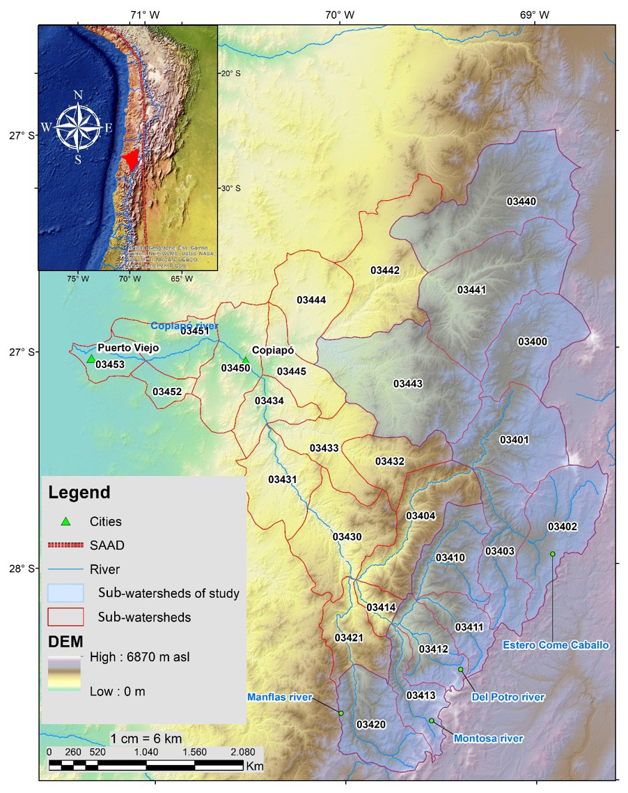
Figure 1 Location map of the Copiapó watershed and the different sub-watersheds (Zone 19S). The codes in each sub-watershed represent the official numbering that the General Water Directorate assigns to each sub-watershed. Basemap: Esri, Maxar, Earthstar Geographics, and the GIS User Community | Powered by Esri.

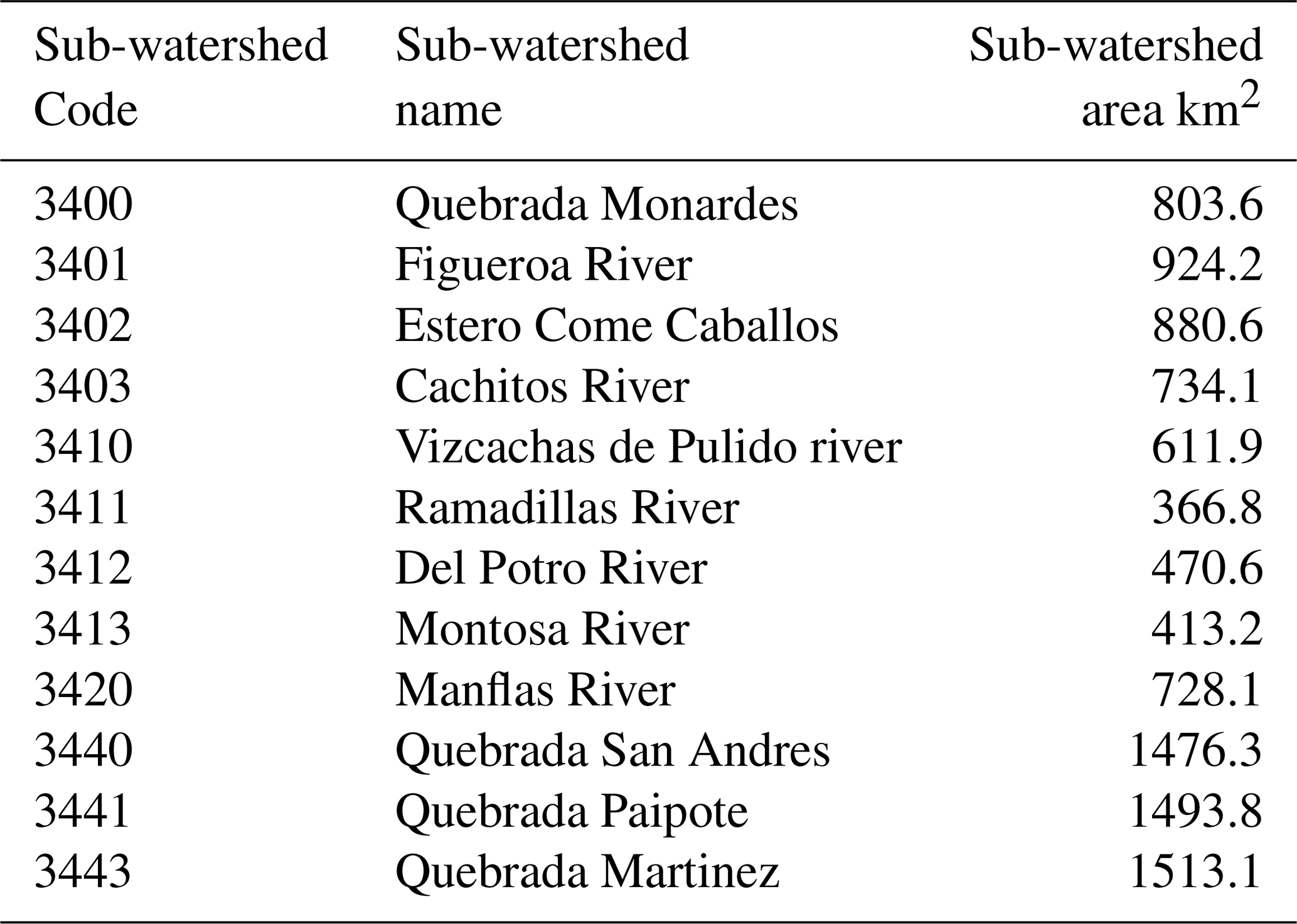
Table 1 List of sub-watersheds with cryospheric components in the study area.

2 Regional setting

2.1 Study Area

The Copiapó watershed is composed of 27 sub-watersheds, distributed along the high mountain belt that forms the headwaters. A sub-watershed is defined here as a watershed unit with a lower Strahler stream order than the main watershed. In our research area, the Copiapó watershed corresponds to the main watershed and contains rivers with a maximum Strahler stream order of nine. Within this hierarchy, sub-watersheds draining from the headwaters typically initiate with Strahler orders of one to three and progress downstream until they merge into larger tributaries with stream orders of up to nine. By distinguishing among sub-watersheds and their associated cryospheric landforms, we can perform both quantitative and qualitative assessments of the current potential water volumes stored within cryospheric environments.

To classify a sub-watershed as a cryospheric watershed, we applied objective and reproducible criteria based on its cryospheric components. A sub-watershed is considered cryospheric only when it fulfilled two conditions: (i) the presence of at least one active cryospheric landforms (debris-free glacier, debris-covered glacier, rock glacier, protalus lobe, or gelifluction taluses) mapped in the regional inventory of glaciers and the periglacial environment of the Atacama Desert (García et al., 2017); and (ii) measurable seasonal snow, expressed as long-term snow permanence derived from MODIS fractional snow cover (Rittger et al., 2013). Sub-watersheds fulfilling both requirements (≥1 cryospheric landforms + snow permanence) were classified as cryospheric.

Applying these criteria resulted in 12 sub-watersheds being identified as cryospheric watersheds (Fig. 1; Table 1). These sub-watersheds are located entirely within high-elevation sectors of the Copiapó watershed (mean elevation 3617 m a.s.l.), coincide with areas of high permafrost probability in the global permafrost model of Gruber (2012), and contain 97 % of the cryospheric landforms mapped in the Copiapó watershed. This classification is therefore geomorphologically justified, reproducible, and consistent with independent permafrost modelling and regional cryospheric inventories.

The Copiapó watershed (Fig. 1) is located in the southern limit of the Atacama Desert, the driest desert of the world (Clarke, 2006), near to the South American Arid Diagonal or SAAD (Zech et al., 2008). The annual precipitation in Copiapó from 1795 to the present has an annual mean of 22.5 mm (Izquierdo et al., 2024). Among the arid watersheds in northern Chile, the Copiapó watershed is regarded as one of the most vulnerable (Suárez et al., 2014). Because of the limited availability of freshwater and the overexploitation of superficial water and groundwater, the deepening of the water table is accelerating and cryospheric landforms and snow are reducing (Casassa et al., 2007; Vuille et al., 2008). Despite this very limited liquid precipitation in the lower areas, e.g. around the city of Copiapó, there is a flow of water in the rivers of the Copiapó watershed year round. This water comes from the Andean cryosphere that is known to host and store large amounts of fresh water (Bolch and Marchenko, 2009; Bórquez et al., 2006; Azócar and Brenning, 2010; Schaffer et al., 2019).

The glacial and periglacial inventory of the Copiapó watershed indicates a transition from areas that are dominated by glacial environments in the south, to areas that are dominated by periglacial environments in the north (García et al., 2017). In the Copiapó watershed, the occurrence of snow begins above 3500 m of altitude. In these extreme environments, the water budget is significantly influenced by snow sublimation. From 2001 to 2016, approximately 70 % of the snow balance was lost to sublimation, effectively reducing the available water volume (Jara et al., 2021). In semi-arid regions of Chile and Argentina, snow accumulation and subsequent melt processes contribute substantially to surface runoff in numerous Andean River Watersheds (Masiokas et al., 2006; Favier et al., 2009).

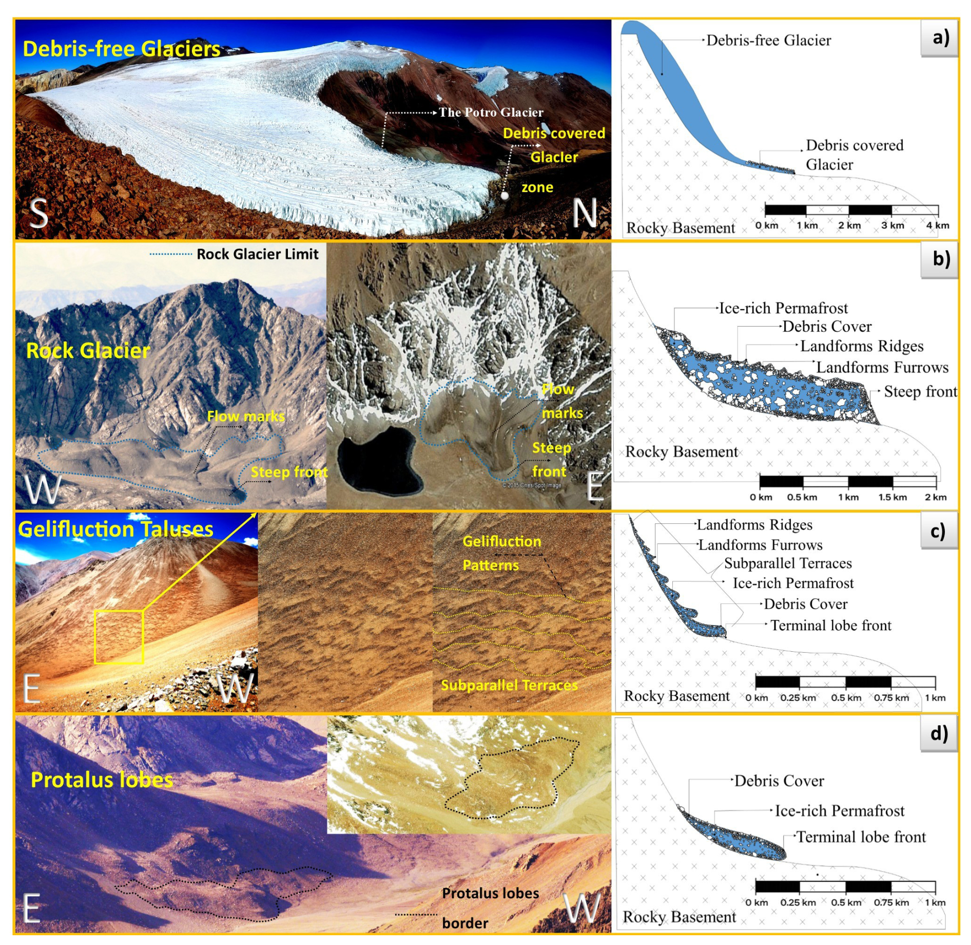
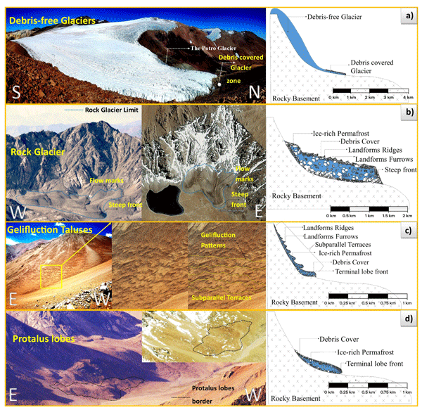
Figure 2 Main cryospheric landforms. Field photographs from the Copiapó Watershed on the left, with a schematic interpretation on the right of. (a) Debris-free glacier and debris-glaciers, (b) Rock glaciers of the Del Potro River Sub-watershed. (c) Gelifluction taluses of Montosa River Sub-watershed, (d) Protalus lobes of the La Laguna Sub-watershed in Vizcachas de Pulido Sub-watershed. Basemap in panels (b) and (d): Esri, Maxar, Earthstar Geographics, and the GIS User Community | Powered by Esri.

2.2 Hydrological background of the cryosphere and conceptual framework for ice-volume estimation

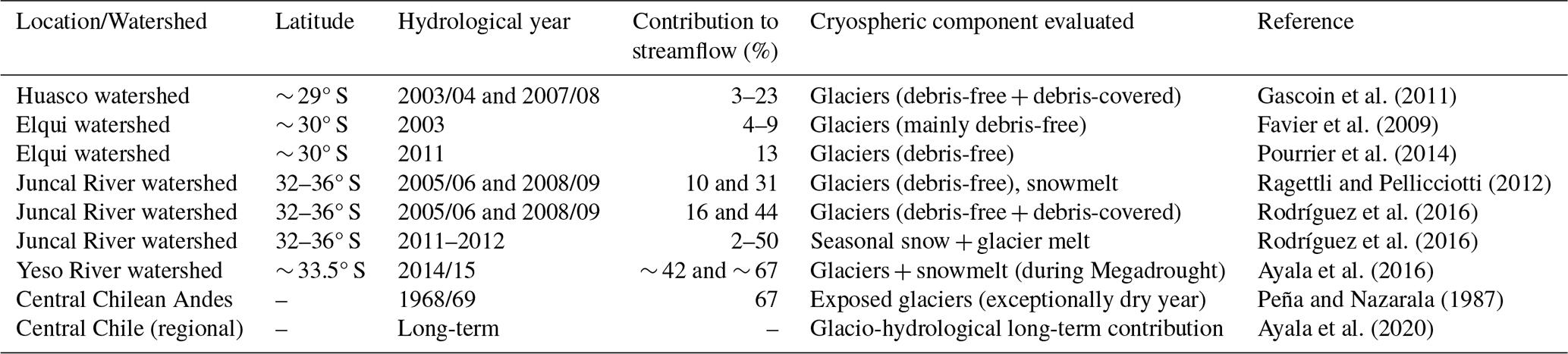
The hydrology of arid Andean Watersheds is dominated by cryospheric processes. In the Copiapó watershed, year-round streamflow persists despite minimal precipitation at mid- to low elevations, indicating that meltwater from snow, glaciers, and ice-rich permafrost constitutes the primary source sustaining discharge. Long-term records from the Dirección General de Aguas (DGA) hydrometric network show a pronounced summer peak in river flow, when rainfall is nearly zero, together with a high baseflow index, confirming a melt-dominated regime and the central hydrological role of the cryosphere in this region. These patterns are consistent with previous studies across the semi-arid Andes (Favier et al., 2009; Gascoin et al., 2011; Ayala et al., 2016), where snow and frozen water bodies act as short- and long-term ice storage modulating runoff during dry years (Table 2).

Cryospheric contributions, however, operate over markedly different response times. Seasonal snow responds at sub-seasonal scales, controlling the onset and magnitude of spring–summer discharge. Debris-free and debris-covered glaciers respond at seasonal to multiannual scales, providing sustained meltwater even in years of limited snowfall. Ice-rich permafrost landforms, including rock glaciers, protalus lobes, and gelifluction taluses, contribute at decadal to centennial scales and represent the most climatically buffered ice storage in the watershed. Capturing these contrasted response times requires not only quantifying the spatial distribution of cryospheric landforms but also applying a coherent conceptual framework for estimating their ice volumes.

The classification of debris-covered glaciers adopted in this study follows Kirkbride (2011), who defines them as glaciers whose ablation zone is largely or entirely covered by supraglacial debris across its full width. This distinction is important in the study area, where debris-covered glaciers occur in close spatial association with rock glaciers but represent fundamentally different cryospheric processes: debris-covered glaciers are dynamic ice bodies in which the supraglacial covered modulates ablation, whereas rock glaciers are permafrost landforms whose movement is driven by internal ice deformation in an ice-rich debris matrix.

Table 2 Contribution to streamflow (%) indicates the proportion of total river discharge supplied by cryospheric meltwater (glaciers and/or seasonal snow), as quantified in each study. Modified from Schaffer et al. (2019).

Estimating ice volume in mountain cryospheric systems relies on methodological approaches that vary in complexity, physical basis, and data requirements. Traditionally, regional and global assessments have applied empirical area–volume or area–thickness relationships (e.g., Bahr et al., 1997; Jones et al., 2018). These models provide valuable first-order estimates and remain particularly useful in data-sparse regions. However, by construction, they do not explicitly account for glacier geometry, internal deformation, thermal regime, or spatially variable creep rates, which are processes that exert strong control on ice thickness in both glacial and periglacial landforms.

More recent advances have increasingly emphasized physically based approaches that better represent the mechanics of glacier flow and permafrost creep. For debris-free glaciers, inversion techniques such as the model designed by Farinotti et al. (2017) combine mass conservation, surface slope, and Glen's flow law to derive spatially distributed ice thicknesses (Fig. 3), and form the basis of the global consensus thickness product of Farinotti et al. (2019). At continental scales, Millan et al. (2022) further demonstrated the value of integrating satellite-derived surface velocities into ice-flow inversion, substantially refining glacier thickness estimates and highlighting the importance of kinematic constraints.

In parallel, physically informed modelling has also progressed for ice-rich permafrost landforms. Viscoplastic formulations, such as those proposed by Cicoira et al. (2021), explicitly link surface velocity, basal shear stress, rheology, and thermal conditions to estimate the thickness of ice-rich layers in rock glaciers. Building on these concepts, Hu et al. (2023) applied deformation-based approaches to regional rock-glacier inventories, illustrating the feasibility of estimating ice content in permafrost landforms using remote sensing–derived kinematics. These developments reflect a broader methodological shift toward deformation-based, physically constrained estimates of ice volume across both glacial and periglacial environments.

In the Andes, the applicability of these physically based approaches is reinforced by the growing availability of satellite-derived deformation data. For example, Villarroel et al. (2018) used Sentinel-1 DInSAR to map surface displacement of more than 2100 rock glaciers in the Dry Andes, while Vidal-Páez et al. (2024) applied PAZ-SAR SBAS-DInSAR to detect millimetric rock-glacier motion in the Chilean Andes. Together, these studies demonstrate that interferometric and feature-tracking techniques enable the detection of low-magnitude deformation, allowing thickness estimation even in low-creep permafrost landforms such as protalus lobes and gelifluction taluses.

In this study, we adopt an integrated conceptual framework that applies:

1. the physically based Farinotti model to debris-free glaciers;

2. a geometry-consistent approach for debris-covered glaciers using thickness gradients from Farinotti et al. (2019); and

3. a unified viscoplastic formulation (Cicoira et al., 2021) to all permafrost cryospheric landforms including rock glaciers, protalus lobes, and gelifluction taluses supported by DInSAR-derived velocities.

This unified framework ensures physical consistency across cryospheric landforms with contrasting dynamics and provides the conceptual foundation required for robust estimation of cryospheric ice volumes prior to their integration into the Normalized Cryospheric Index (NCI).

2.3 Glacier and Periglacial Environment

The Copiapó watershed hosts a diverse assemblage of cryospheric landforms (Fig. 2), including debris-free glaciers, debris-covered glaciers, rock glaciers, gelifluction taluses, and protalus lobes, as documented in the regional inventory of García et al. (2017). These landforms exhibit a marked spatial variability across the watershed, reflecting strong controls by elevation and topography.

Based on the regional inventory of García et al. (2017), a total of 1862 cryospheric landforms have been mapped within the Copiapó watershed: 62 debris-free glaciers, 16 debris-covered glaciers, 173 rock glaciers, 848 gelifluction taluses, and 763 protalus lobes. Gelifluction taluses (46 %) and protalus lobes (41 %) thus dominate the cryospheric assemblage of the watershed, while debris-free and debris-covered glaciers together account for less than 4 % of the inventoried landforms. This numerical distribution reinforces the periglacial character of the Copiapó cryosphere and underscores the relevance of ice-rich permafrost landforms for ice-volume estimations at the watershed scale. This inventory was not originally developed under the Randolph Glacier Inventory (RGI) framework, as it predates the standardization of global glacier datasets in the study region. Instead, the inventory provides a detailed regional mapping of cryospheric landforms, including not only glaciers but also ice-rich permafrost features such as rock glaciers, gelifluction taluses, and protalus lobes. This distinction is particularly relevant because global glacier inventories, such as RGI, are primarily focused on glacier ice bodies and typically do not include periglacial landforms, which are rarely mapped in a systematic manner. As a result, the regional inventory used here captures a broader spectrum of cryospheric components that are especially significant in arid mountain environments, where non-glacial frozen water storage may play an important hydrological role.

In general, cryospheric landforms are distributed discontinuously along the high Andes, with notable differences between northern and southern sectors. In areas such as Nevado Jotabeche and Los Tronquitos, landforms are predominantly located on high-elevation ridges and peaks, whereas in the Del Potro region they are more commonly confined to valley bottoms between steep slopes.

Gelifluction taluses represent one of the most widespread landforms in the study area and are typically associated with high-elevation environments. In the southern sector, they frequently occur in close proximity to debris-free glaciers, forming coupled glacial–periglacial systems. In contrast, in the northern sector, gelifluction features tend to appear as smaller and more isolated landforms.

Rock glaciers are mainly distributed along steep valley flanks at intermediate to high elevations, often occupying topographic depressions or confined valley settings. Debris-free glaciers are generally restricted to the highest elevations and, particularly in the southern sector, are commonly associated with adjacent periglacial landforms.

Protalus lobes are especially abundant in some northern areas, where they develop on slopes of varying gradients and exhibit a range of sizes and morphologies. Debris-covered glaciers are comparatively scarce and are typically found in the southern sector, occurring as small bodies located downslope of debris-free glaciers.

Overall, the distribution of cryospheric landforms in the Copiapó watershed reflects a transition from glacial-dominated systems in the south to predominantly periglacial environments in the north, consistent with regional climatic and topographic gradients (Fig. 4).

The regional inventory of García et al. (2017) predates the RGIK (Rock Glacier Inventories and Kinematics; IPA Action Group) guidelines, but its mapping workflow multi-source satellite photo-interpretation supported by field reconnaissance, identification of active rock glaciers from diagnostic geomorphological criteria (frontal ramp, furrows and ridges), and a GLIMS-compatible attribute database is methodologically consistent with the principles later codified by RGIK. The inventory extends this scope to include gelifluction taluses and protalus lobes, two ice-rich permafrost landforms that dominate the arid Atacama cryosphere but fall outside the RGIK rock-glacier framework.

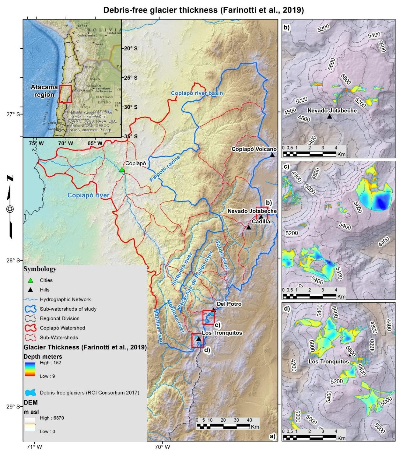
Figure 3 (a) Distribution map of the debris-free glacier thickness from Farinotti et al. (2019). (b) Jotabeche Volcano cryospheric landforms distribution (c) The Del Potro Hill cryospheric landforms distribution (d) The Tronquitos Hill cryospheric landforms distribution. Basemap: Esri, Maxar, Earthstar Geographics, and the GIS User Community | Powered by Esri.

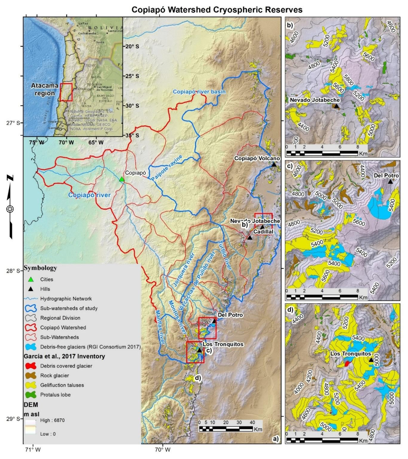
Figure 4 (a) Distribution map of the cryospheric landforms inventoried in the Atacama region from García et al. (2017). (b) Jotabeche Volcano cryospheric landforms distribution (c) The Del Potro Hill cryospheric landforms distribution (d) The Tronquitos Hill cryospheric landforms distribution. Basemap: Esri, Maxar, Earthstar Geographics, and the GIS User Community | Powered by Esri.

3 Methodology

3.1 Survey of cryospheric landforms

To quantify the ice volume in the Copiapó watershed, we used existing cryospheric inventories without performing new delineations. The regional inventory of glaciers and periglacial landforms of the Atacama Desert (García et al., 2017) was employed directly to extract polygons of debris-covered glaciers, rock glaciers, protalus lobes, and gelifluction taluses. This inventory represents the only comprehensive and validated dataset that explicitly identifies periglacial cryospheric landforms in northern Chile, and its polygons were incorporated without modification into our analysis.

Debris-free glaciers were obtained exclusively from the Randolph Glacier Inventory (RGI) v6.0 (RGI Consortium, 2017). For these glaciers, we did not compute ice thickness ourselves. Instead, we used the pre-computed global ice-thickness product of Farinotti et al. (2019), which is physics-based and already calibrated on RGI glacier outlines (Fig. 3). Because the Farinotti model requires RGI geometry as input, the use of RGI v6.0 ensures direct compatibility with the global thickness dataset. Ice volumes for debris-free glaciers were therefore calculated solely by spatially integrating the published Farinotti et al. (2019) thickness values over the RGI glacier polygons within the Copiapó watershed. This approach avoids any reinterpretation of glacier geometry or re-estimation of ice thickness, ensuring methodological transparency and consistency with the global consensus product.

The joint use of the inventory developed by García et al. (2017) and RGI v6.0 glacier inventory is thus complementary. RGI provides standardized glacier boundaries and their associated Farinotti-derived thickness fields for debris-free glaciers, whereas García et al. (2017) provides the spatially explicit identification of debris-covered glaciers and periglacial landforms that are not represented in global glacier datasets. By relying directly on these inventories and on the published model outputs of Farinotti et al. (2019), our workflow remains fully reproducible and avoids introducing new mapping or thickness-estimation steps.

Mapping uncertainty for all polygons was propagated using the one-pixel boundary buffer method of Paul et al. (2013), ensuring consistent treatment of spatial uncertainty across glacial and periglacial cryospheric landforms.

3.2 Survey of snow cover: MODIS-derived snow permanence

The MOD10A1 Fractional Snow Cover (FSC) product from NASA was used to characterize snow based on long-term patterns of snow permanence. Each MOD10A1 image provides, for every 500 × 500 m pixel, a value representing the fractional snow cover within that pixel (from 0 to 1), derived through a spectral unmixing algorithm (Rittger et al., 2013). This sub-pixel representation allows a more accurate depiction of discontinuous or patchy snow, which is common in high-elevation arid regions. Instead of relying on isolated scenes, we processed the complete daily MODIS time series (2000–2022) to obtain both the instantaneous snow-covered area and the frequency of snow permanence at the sub-watershed scale. Although cloud contamination can introduce occasional misclassifications, the product maintains approximately 90 % accuracy under ideal conditions (Hall et al., 2002; Pan et al., 2024), and is suitable for long-term characterization of snow permanence.

From the daily FSC series, each MODIS image provides the fractional snow cover for every 500 × 500 m pixel. Using this long-term record, fractional snow cover (FSC) was used as the core variable to represent the proportion of snow within each pixel in each scene. In addition, we calculated snow permanence as the fraction of days during the 23-year period in which each pixel exhibited snow-covered conditions according to its FSC value. Snow permanence is therefore not an independent MODIS layer, but a temporal aggregation derived directly from the daily FSC maps, summarizing the frequency and recurrence of snow presence across the watershed.

In this framework, FSC was used as the primary input for constructing long-term mean FSC maps. For each pixel, the daily FSC values were averaged over the full 2000–2022 record to obtain a time-mean fractional snow cover. This per-pixel mean FSC was then multiplied by the pixel area (0.25 km² for the 500 × 500 m MODIS grid) and summed across all pixels within each sub-watershed to yield a mean snow-covered area in km². It is this spatially integrated snow-covered area (km²) that is incorporated into the Normalized Cryospheric Index (NCI) as the indicator of short-term cryospheric water resources, ensuring that both the fractional snow signal at the pixel level and the spatial extent of the sub-watershed are accounted for in the index.

3.3 Field work for ground truthing

Since the mapping workflow is primarily based on remote sensing, satellite imagery, and existing cryospheric inventories, we incorporated targeted field observations and independent geophysical datasets to validate both the identification of cryospheric landforms and the ice-thickness values used in this study. Fieldwork was carried out in the Montosa (03413) and Del Potro (03412) sub-watersheds, which together represent approximately 10 % of the Copiapó watershed and contain accessible examples of the main cryospheric landforms present in the region.

During these campaigns, photographic and geomorphological observations were conducted to verify the surface expression of mapped cryospheric landforms, including gelifluction taluses, protalus lobes, and rock glaciers. These observations allowed us to assess the representativeness of the polygons obtained from existing inventories.

Beyond surface verification, independent geophysical datasets were used to constrain and validate ice-thickness estimates. For debris-free glaciers, ice thickness values from the Farinotti et al. (2019) global product were compared against airborne ground-penetrating radar (GPR) profiles collected by the Dirección General de Aguas (DGA, 2014) over the Del Potro and Tronquitos glaciers.

For ice-rich permafrost landforms, Electrical Resistivity Tomography (ERT) measurements were conducted on a representative gelifluction taluses and on an active rock glacier within the Montosa sub-watershed. These ERT profiles constrain the depth and continuity of ice-rich layers and support the thickness ranges adopted for periglacial cryospheric landforms in the modelling framework.

Together, these field observations and geophysical datasets provide independent validation for both the spatial delineation and the subsurface characteristics of cryospheric landforms within the Copiapó watershed, strengthening the robustness of the ice-volume estimates applied in this study.

3.3.1 Geophysical survey on gelifluction taluses and rock glaciers

Electrical Resistivity Tomography (ERT) was employed to characterize subsurface ice-rich layers in selected periglacial landforms and to provide observational constraints for the ice-thickness values used in the modelling framework. ERT is a multi-electrode resistivity method that generates 2-D vertical sections of the subsurface by injecting electrical current into the ground and measuring the resulting potential differences across electrode arrays. The field configuration used in this study (Table 3) consisted of 36 electrodes operated with Wenner, Schlumberger, and Dipole–Dipole arrays.

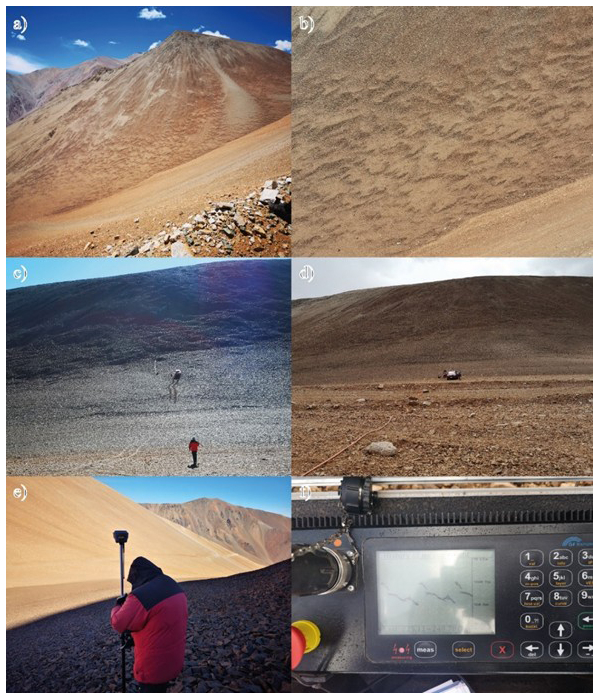
Figure 5 Photography of the fieldwork. (a) And (b) the Lobulated morphology of studied gelifluction taluses, which are not covered in snow; (c) and (d) the geoelectric line cable; (e) and (f) the used equipment, differential GPS and resistivity meter ARES II measuring a resistivity point diagram distribution.

Fieldwork focused on two representative cryospheric landforms within the Montosa sub-watershed: a gelifluction taluses and an active rock glacier (Figs. 5 and 6). These sites were selected because they exhibit clear geomorphological indicators of ice-rich permafrost and provide suitable access for geophysical surveys. The ERT profiles allowed direct identification of high-resistivity zones (>20–50 kΩ ⋅ m), characteristic of massive or highly saturated ice-rich permafrost bodies.

Table 3 Used geophysical equipment for fieldwork of this study.

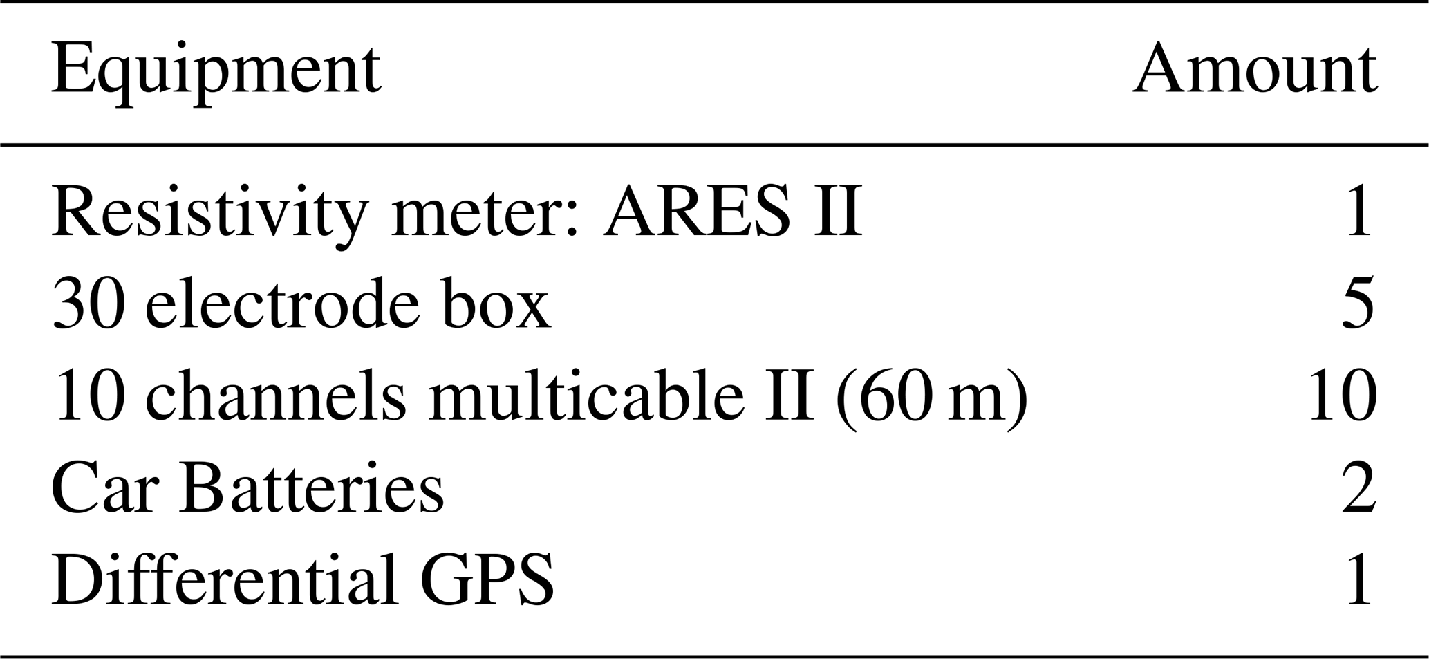
The survey layout required a 600 m profile organized through multicables arranged at 90° angles. A high-precision differential GPS (“South Galaxy”) was used to set the start and end points of each line, ensuring alignment and minimizing installation error. Electrode spacing was fixed at 5 m, with position control verified using a combination of GPS and measured markers at 30 m intervals. All electrodes were tested prior to each acquisition, and any with unacceptable standard deviation values were repositioned.

These ERT measurements provide direct ground validation of subsurface ice for both gelifluction taluses and rock glaciers, supporting the thickness ranges applied to ice-rich permafrost cryospheric landforms in our volume estimations and complementing the GPR-based glacier-thickness validation described in Sect. 3.3.

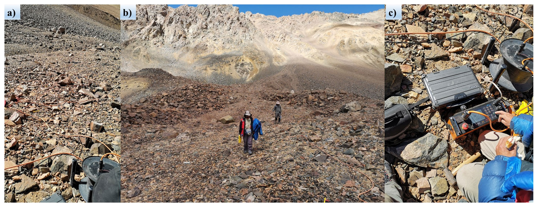
Figure 6 Photography of the fieldwork rock-glacier surface. (a) Intelligent multi-electrode cable reel used for deploying the ERT array across the periglacial terrain. (b) Installation of the 600 m geoelectric line. (c) Operation of the ARES II resistivity meter during data acquisition.

Before every measurement, all electrodes were tested to detect electrodes with high standard deviation in resistivity. If the deviation exceeded acceptable limits, the electrodes were repositioned until the deviation fell within an acceptable range to ensure measurement accuracy.

3.4 DInSAR kinematic analysis for periglacial cryospheric landforms

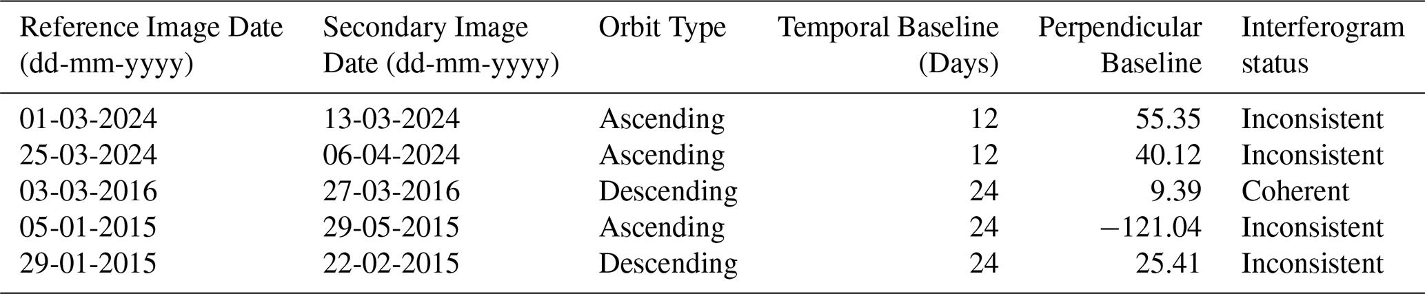
To characterize surface deformation across glacial and periglacial cryospheric landforms and to provide kinematic constraints for ice-thickness modelling, we processed Sentinel-1 IW Single Look Complex (SLC) images using the ESA SNAP v9.0 toolbox. Interferometric pairs were selected based on perpendicular baselines <150 m and temporal baselines <24 d to ensure coherence in high-altitude terrain (Table 4).

Table 4 Sentinel-1 interferometric image pairs and associated temporal and perpendicular baselines tested.

SLC scenes were co-registered using the TOPS burst co-registration workflow. Interferograms were generated, filtered using a Goldstein filter (α = 0.8), and corrected for topographic phase using the 30 m SRTM DEM. Phase unwrapping was performed with SNAPHU in external mode. Line-of-sight (LOS) displacement was obtained from the unwrapped phase:

$$\begin{array}{}\text{(1)}& d_{\mathrm{LOS}}={\displaystyle \frac{\mathit{\lambda }}{\mathrm{4}\mathit{\pi }}}\mathrm{\Delta }\mathit{\varphi }\end{array}$$

Mean surface velocities were extracted for each cryospheric landforms polygon (debris-free glaciers, debris-covered glaciers, rock glaciers, protalus lobes, gelifluction taluses). These DInSAR-derived velocities were incorporated as dynamic constraints for the viscoplastic modelling of permafrost cryospheric landforms and as supplementary kinematic information in glacier-thickness interpretation.

3.4.1 Velocity uncertainty

Uncertainty in DInSAR-derived surface velocity was incorporated by explicitly estimating the phase noise associated with interferometric coherence and temporal baseline. Following Hanssen (2001), the standard deviation of the interferometric phase for a multilooked interferogram is:

$$\begin{array}{}\text{(2)}& {\mathit{\sigma }}_{\mathit{\varphi }}\approx \sqrt{{\displaystyle \frac{\mathrm{1}-{\mathit{\gamma }}^{\mathrm{2}}}{{\mathit{\gamma }}^{\mathrm{2}}L}}}\end{array}$$

Where γ is the interferometric coherence and L the number of equivalent looks. For Sentinel-1 SLC data used in this study, the typical modeled coherence is γ≈0.97, the temporal baseline is Δt = 24 d, and the radar wavelength is λ=0.0555 m.

Phase noise is converted to line-of-sight displacement noise using:

$$\begin{array}{}\text{(3)}& {\mathit{\sigma }}_{\mathit{\varphi }}={\displaystyle \frac{\mathit{\lambda }}{\mathrm{4}\mathit{\pi }}}{\mathit{\sigma }}_{\mathit{\varphi }}\end{array}$$

And subsequently velocity uncertainty:

$$\begin{array}{}\text{(4)}& {\mathit{\sigma }}_{\mathit{\upsilon }}={\displaystyle \frac{{\mathit{\sigma }}_d}{{\mathrm{\Delta }}_t}}={\displaystyle \frac{\mathit{\lambda }}{\mathrm{4}\mathit{\pi }\mathrm{\Delta }t}}\sqrt{{\displaystyle \frac{\mathrm{1}-{\mathit{\gamma }}^{\mathrm{2}}}{{\mathit{\gamma }}^{\mathrm{2}}L}}}\end{array}$$

For a representative multilooking a factor of L=20 was applied. The resulting uncertainties are:

$$\begin{array}{c}{\displaystyle }{\mathit{\sigma }}_{\mathit{\varphi }}\approx \mathrm{0.056}\mathrm{rad},{\mathit{\sigma }}_d\approx \mathrm{2.5}\times {\mathrm{10}}^{-\mathrm{4}}\mathrm{m}=\mathrm{0.25}\mathrm{mm},\\ {\displaystyle }{\mathit{\sigma }}_d\approx \mathrm{1.0}\times {\mathrm{10}}^{-\mathrm{5}}\mathrm{m}{\mathrm{d}}^{-\mathrm{1}}=\mathrm{0.01}\mathrm{mm}{\mathrm{d}}^{-\mathrm{1}}\approx \mathrm{3}\text{–}\mathrm{4}\mathrm{mm}{\mathrm{yr}}^{-\mathrm{1}}\end{array}$$

This value (σ_d=0.01 mm d⁻¹) was thus adopted as the 1σ uncertainty of DInSAR velocity measurements.

3.5 Calculation of the ice volume and uncertainty

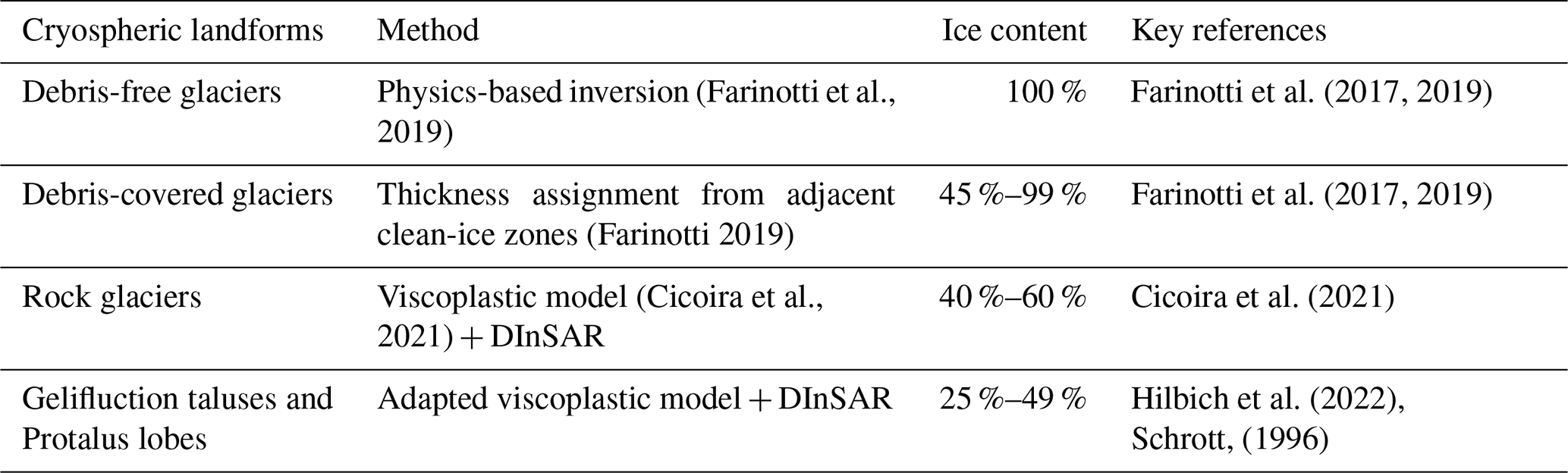
To quantify the total ice volume stored in glacial and periglacial cryospheric landforms, we applied cryospheric landforms-specific physics-based models according to their mechanics, morphology, and available input data (Table 5). The method applied and associated uncertainties are detailed below.

3.5.1 Debris-free glaciers

Ice thickness for debris-free glaciers was obtained from the global consensus ice-thickness dataset of Farinotti et al. (2019), which integrates multiple physics-based inversion models (Farinotti et al., 2017). Glacier volumes were computed by spatially integrating the consensus ice-thickness rasters over the RGI v6.0 glacier polygons within the Copiapó watershed. A relative uncertainty of ±26 % was applied following the uncertainty assessment reported in Farinotti et al. (2017, 2019).

3.5.2 Debris-covered glaciers

Mean ice thickness for debris-covered glaciers was derived by sampling the Farinotti et al. (2019) consensus ice-thickness field in the clean-ice frontal zones immediately adjacent to each debris-covered area. These representative values were then assigned to the corresponding debris-covered glacier polygons, ensuring consistency with the local glacier geometry and thickness gradients. Ice volumes were calculated by multiplying the assigned mean thickness by the mapped debris-covered glacier area. Due to the inherently greater spatial variability and additional uncertainties associated with debris cover (e.g., variations in debris thickness, thermal properties, and remote-sensing–derived thickness estimates), published studies of debris-covered glacier thickness consistently report substantially larger differences between modeled and in situ measurements compared to debris-free glaciers (e.g. ∼ 40 % uncertainty for certain debris-covered glaciers; see Pieczonka et al., 2018). Hence, a conservative uncertainty of ±35 % was adopted for debris-covered glacier volume estimates to account for these factors.

3.5.3 Rock glaciers

Rock-glacier thickness was estimated using a viscoplastic creep inversion following Cicoira et al. (2021), where basal shear stress is constrained by observed surface velocity. For each rock glacier, mean slope-parallel surface velocities (v) and their standard deviation (σ_v) were derived from Sentinel-1 DInSAR measurements (Sect. 3.4.1) and expressed in m yr⁻¹. The basal shear stress τ was inverted using the 1-D viscoplastic formulation with Glen-type exponent n=3 and a temperature-dependent rate factor (T).

To explicitly represent uncertainty in the thermal state of ice-rich permafrost in the Central Andes, we treated ice temperature as a normal distribution:

$$\begin{array}{}\text{(5)}& T\sim N(-\mathrm{3},\mathrm{3}\mathrm{°}\mathrm{C})\end{array}$$

This choice is consistent with reported near-isothermal to moderately cold permafrost conditions in the Central Andes, including rock-glacier settings, and with the strong temperature sensitivity of creep close to 0 °C described in constitutive studies (e.g. Koenig et al., 2025; Monnier and Kinnard, 2013).

Using τ, mean thickness was computed as:

$$\begin{array}{}\text{(6)}& H={\displaystyle \frac{\mathit{\tau }}{\mathit{\rho }\cdot g\cdot \sin \left(\mathit{\alpha }\right)}}\end{array}$$

where α is the mean surface slope, ρ is ice density, and g is gravitational acceleration. Total landform volume was computed as:

$$\begin{array}{}\text{(7)}& V=A\cdot H\end{array}$$

where A is the mapped planimetric area.

Ice volume was obtained by applying an ice-content fraction C_I? to the landform volume:

$$\begin{array}{}\text{(8)}& V_{\mathrm{ice}}=V\times C_{\mathrm{I}}\end{array}$$

For rock glaciers, C_I was represented as a bounded range consistent with reported values for these type of ice-rich permafrost landforms (Cicoira et al., 2021):

$$\begin{array}{}\text{(9)}& C_{\mathrm{I}}=\mathrm{0.5}\pm \mathrm{0.10}\end{array}$$

Ice mass (in Gt) was then computed as:

$$\begin{array}{}\text{(10)}& M_{\mathrm{Gt}}={\displaystyle \frac{V_{\mathrm{ice}}\mathit{\rho }}{{\mathrm{10}}^{\mathrm{12}}}}\end{array}$$

with $\mathit{\rho }=\mathrm{900}\pm \mathrm{20}$ kg m⁻³. Uncertainties in H and M_Gt were propagated from σ_v, σ_T, slope uncertainty, mapping uncertainty in area, ice-content uncertainty, and density uncertainty using quadratic propagation of relative errors (Sect. 3.5.5).

3.5.4 Protalus lobes and gelifluction taluses

Protalus lobes and gelifluction taluses were modelled using the same viscoplastic inversion framework originally developed for rock glaciers (Cicoira et al., 2021), exploiting low but measurable DInSAR-derived surface deformation to constrain basal shear stress and thickness. For each mapped polygon, mean slope-parallel surface velocity and its associated uncertainty (v, σ_v) were used to invert basal shear stress and compute thickness H through Eq. (6). Thermal uncertainty was represented using the same Central Andes temperature prior described in Eq. (5).

However, in contrast to rock glaciers, protalus lobes and gelifluction taluses are characterized by lower ice contents, higher debris fractions, and a dominance of seasonal or shallow permafrost deformation mechanisms. To account for these rheological differences, we modified the Glen-type flow exponent n used in the inversion. While rock glaciers were modelled assuming n=3, consistent with creep-dominated ice–debris mixtures (Cicoira et al., 2021), protalus lobes and gelifluction taluses were modelled using a reduced exponent (n=2), reflecting more linear, frictionally controlled deformation regimes typical of ice-poor frozen debris slopes. This adjustment reduces the sensitivity of inferred thickness to surface velocity and avoids unrealistically thick solutions for low-velocity landforms.

Because ice contents in these landforms are generally lower and more heterogeneous than in rock glaciers, ice-content fraction was prescribed following Eq. (11) as a bounded prior range rather than a fixed value. This range represents plausible ground-ice fractions for ice-rich permafrost slopes in the Central Andes and is supported by field-calibrated ERT observations showing strong spatial variability in ground-ice content within Andean permafrost landforms (Hilbich et al., 2022), as well as early empirical constraints for frozen debris slopes in arid mountain environments (Schrott, 1996). The ice-content prior was therefore implemented to represent structural uncertainty rather than a deterministic parameter.

$$\begin{array}{}\text{(11)}& C_{\mathrm{I}}=\mathrm{0.37}\pm \mathrm{0.12}\end{array}$$

Following thickness estimation, landform volume was computed using Eq. (7), ice volume using Eq. (8), and ice mass using Eq. (10).

3.5.5 Uncertainty propagation framework for ice-rich permafrost cryospheric landforms

For rock glaciers, gelifluction taluses, and protalus lobes, uncertainties in ice thickness and ice mass were propagated deterministically using quadratic propagation of relative errors for multiplicative quantities. First, the uncertainty in mapped area was estimated following Paul et al. (2013), assuming boundary errors occur within ±0.5 pixels and using:

$$\begin{array}{}\text{(12)}& u_{A_i}={\displaystyle \frac{\mathrm{1}}{\mathrm{2}}}{P}_i\times \mathit{\lambda }\times \mathit{\sigma }\end{array}$$

where P_i is the polygon perimeter, λ is the spatial resolution of the imagery used for delineation, and σ≈0.6872 is a correction factor corresponding to the standard deviation of a Gaussian distribution with most errors confined within ±0.5 pixels.

Ice volume was computed using the Eq. (7), and ice mass as $M_{\mathrm{Gt}}\propto A\times H\times C_{\mathrm{I}}\times \mathit{\rho }$. Therefore, the relative uncertainty in ice mass was calculated as:

$$\begin{array}{}\text{(13)}& {\left({\displaystyle \frac{{\mathit{\sigma }}_M}{M}}\right)}^{\mathrm{2}}={\left({\displaystyle \frac{{\mathit{\sigma }}_A}{A}}\right)}^{\mathrm{2}}+{\left({\displaystyle \frac{{\mathit{\sigma }}_H}{H}}\right)}^{\mathrm{2}}+{\left({\displaystyle \frac{{\mathit{\sigma }}_{C_{\mathrm{I}}}}{C_{\mathrm{I}}}}\right)}^{\mathrm{2}}+{\left({\displaystyle \frac{{\mathit{\sigma }}_{\mathit{\rho }}}{\mathit{\rho }}}\right)}^{\mathrm{2}}\end{array}$$

and the absolute uncertainty as ${\mathit{\sigma }}_M=M\times \left(\frac{{\mathit{\sigma }}_M}{M}\right)$. Watershed totals were obtained by summing masses across polygons, while total uncertainty was aggregated assuming independence using:

$$\begin{array}{}\text{(14)}& {\mathit{\sigma }}_{\mathrm{tot}}=\sqrt{{\sum }_i^n{\mathit{\sigma }}_{M_i}^{\mathrm{2}}}\end{array}$$

This framework ensures consistent uncertainty propagation across all ice-rich permafrost cryospheric landforms while preserving the physically based dependence of thickness on surface velocity and temperature.

Table 5 Key references used as input for the calculation of ice volumes of cryospheric landforms.

3.6 Cryospheric landforms and snow index and data integration

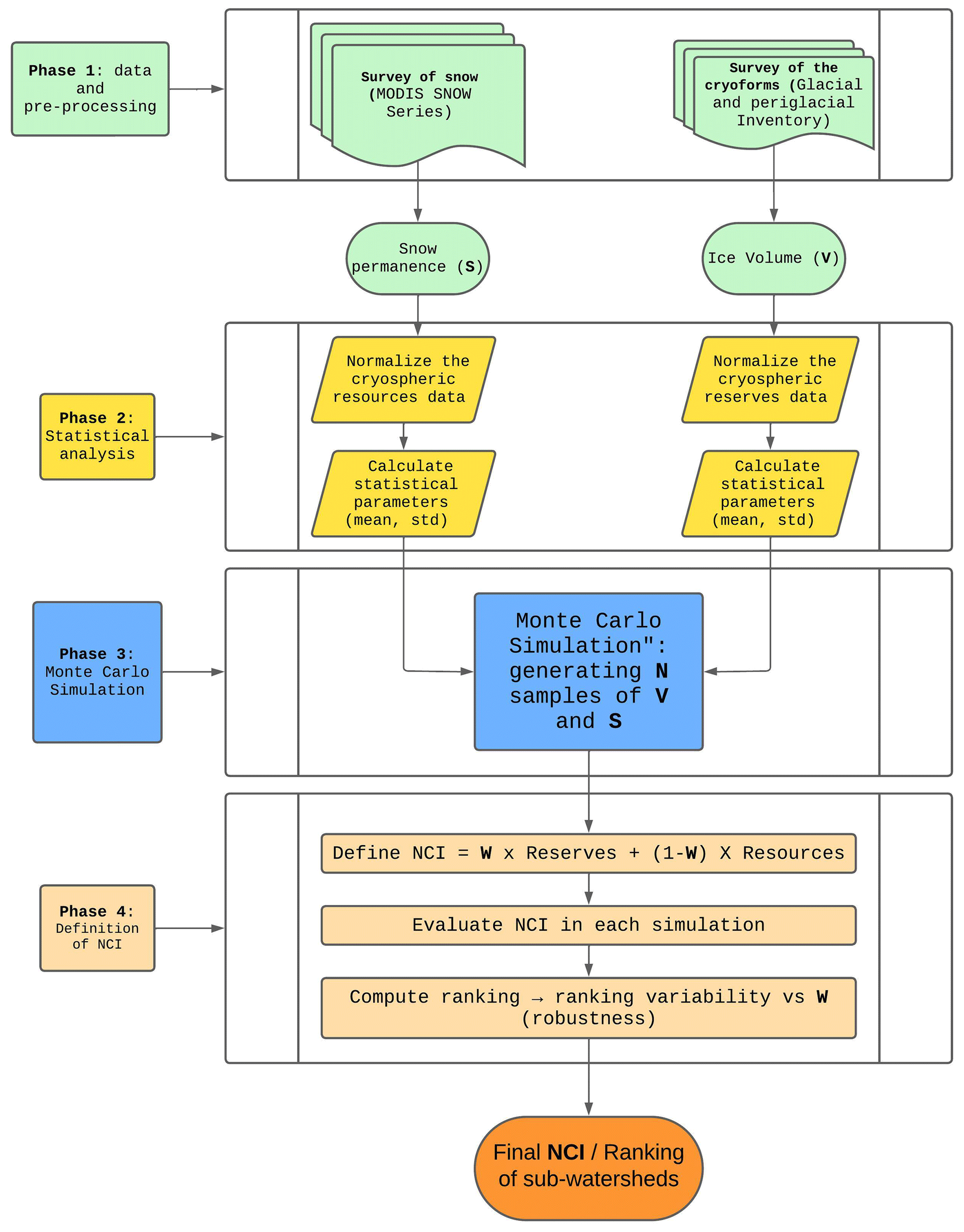
To develop a classification system that categorizes the capacity to store ice as a strategic water reserve in desert areas of sub-watersheds, we followed a workflow that consists of four phases (Fig. 7). We developed the classification system using cryospheric landforms (expressed in gigatons (Gt), equivalent to 1000 million metric tons of ice) and snow (quantified in km² of snow-cover extent), integrating both into the methodological framework. The strategic Normalized Cryospheric Index (NCI) captures the relative significance of each sub-watershed, considering both its ability to store water as ice (cryospheric landforms) and its potential to regenerate water resources through snowfall. The NCI needs to be adapted to each specific case. For the Copiapó watershed, the active cryospheric landforms present until 2024 have been used. Those cryospheric landforms include debris-free glaciers, debris-covered glaciers, rock glaciers, gelifluction talus and protalus lobes. Depending on the types of cryospheric landforms available in a specific region, the number of cryospheric landforms included may vary.

The methodological framework for computing the NCI index integrates Monte Carlo simulation with a robustness assessment of a composite indicator that incorporates ice volume (V) and snow permanence (S), adhering to the uncertainty propagation principles in simulation-based methodologies outlined by Rubinstein and Kroese (2016). First, each watershed has a mean value (e.g., $\stackrel{\mathrm{‾}}{V_i}$ and $\stackrel{\mathrm{‾}}{S_i}$) and an estimate of its dispersion (ΔV_i and ΔS_i), usually understood as standard deviation. On the basis that both V and S follow normal distributions $N(\stackrel{\mathrm{‾}}{V_i},\mathit{\sigma }\mathrm{2}v)$ and $N(\stackrel{\mathrm{‾}}{S_i},\mathit{\sigma }\mathrm{2}s)$, N replicates of each variable are generated for each watershed, thus obtaining “clouds of values” representing the uncertainty of each datum. Subsequently, a normalization is performed (using min-max) in order to avoid that one variable dominates the other only by differences in magnitude.

Once the simulated values are generated, a weighted index is defined whose objective is to combine both variables (Eq. 15):

$$\begin{array}{}\text{(15)}& {\mathrm{NCI}}_{i,k}\left(\mathit{\omega }\right)=\mathit{\omega }-V_{i,k}+\left(\mathrm{1}-\mathit{\omega }\right)-S_{i,k}\end{array}$$

Where $\mathit{\omega }\in [\mathrm{0},\mathrm{1}]$.

Where ω is a parameter that determines the relative relevance of ice volume versus snow permanence. For each sample k (among the N simulations), the values of that index in all the watersheds are obtained and ordered from highest to lowest, giving rise to a specific ranking of each run. In this way, each watershed “i” gets a “position” (1 for the watershed with the highest index, 2 for the next one and so on).

The ranking variability function (Eq. 16) relies on the stability of the ranking under uncertainty, in accordance with the sensitivity analysis framework outlined by Saltelli et al. (2008). Specifically, for each watershed, the standard deviation of its position over the N runs is measured, and this measure of dispersion is summed (or averaged) for all watersheds. A smaller value of this sum indicates greater stability or robustness in the ranking. Formally, if σ_i denotes the standard deviation of the position of watershed under a weight ω, the objective function results:

$$\begin{array}{}\text{(16)}& f\left(\mathit{\omega }\right)={\sum }_{i=\mathrm{1}}^n[{\mathit{\sigma }}_i\cdot (\mathit{\omega }\left)\right]\end{array}$$

Where lower values indicate a more stable ranking. A sweep over [0,1] is performed to evaluate how ranking stability depends on ω. Because ω represents the relative contribution of long-term ice storage versus seasonal snow to runoff, its value is constrained hydrologically rather than statistically: for each hydrological year, ω was estimated as the fraction of October–March discharge at Pastillo not explained by September snow cover, i.e. the intercept of the snow–discharge regression (Fig. 10) divided by the observed mean discharge of that year. This yields an empirical distribution of ω for 2001–2022 (mean 0.43; 0.27 and 0.62 for the wettest and driest tercile of snow years), which is sampled in each Monte Carlo replicate, so that the integrated NCI reflects the observed frequency of wet and dry regimes, while the two terciles define wet-year and dry-year scenarios.

Finally, plots are generated to analyze the resulting average ranking and the probability that certain watersheds occupy the first place in various simulations. In this way, a picture is obtained of how uncertainty in ice volume and snow permanence affects the prioritization of watersheds.

Although the NCI has a simple formulation, the variables it combines are affected by substantial uncertainty. Ice volumes integrate multiple sources of error related to thickness modelling, ice content, density, and mapped area, while snow is represented by long-term snow permanence derived from MODIS, which captures both the spatial extent and temporal recurrence of snow. Monte Carlo simulation is therefore applied not to increase index complexity, but to propagate uncertainty in ice volume and snow permanence into watershed ranking and to evaluate ranking robustness across the hydrologically observed range of the weighting factor. This stochastic framework avoids arbitrary parameterization and ensures a stable, transparent, and reproducible classification of cryospheric sub-watersheds.

Figure 7 Flow chart of the methodology used to calculate the NCI.

4 Results

4.1 Snow permanence results

By integrating all MODIS fractional snow cover images and computing their long-term mean over the period 2000–2022, we derived a snow permanence metric, defined as the probability of snow presence at each pixel. The resulting raster represents the spatial distribution of snow permanence across the Copiapó watershed (Fig. 8). At the regional scale, snow permanence shows limited spatial variability at high elevations, remaining consistently high above approximately 5500 m a.s.l. These regions are located close to the Argentinean border. In the central area between Caserones Hill and Cadillal Hill, no cryospheric landforms were identified, which coincides with the lowest snow permanence values in the study area, with snow present only around 30 % of the time. In contrast, the highest snow permanence values are observed in the southern sector of the study area. In the central area of the Copiapó watershed the snow permanence is concentrated around the Nevado Jotabeche Hill area. The northern part of the watershed does not show concentrated major snowfall anomalies. Snow permanence has persisted approximately 30 %–50 % of the time exclusively at high-elevation zones (>4500 m a.s.l.) near the Argentinian border, contrasting sharply with lower altitudes starting at 2000 m a.s.l.

The calculated probability of the occurrence for the investigated watersheds shows that the snow permanence watershed varies, with higher snow permanence for the southern watersheds compared to the central and northern watersheds. The watershed with the highest resource index is the Montosa River watershed (03413) with 0.18 probability of being covered in snow. The Vizcachas de Pulido River (03410), which is located at the lowest altitude, has the lowest probability of 0.07 to have snow permanence. These per-pixel snow permanence values, when multiplied by the pixel area (0.25 km²) and integrated across each sub-watershed, yield the mean snow-covered area in km² reported in Table 6 and used as the snow variable S in the NCI calculation.

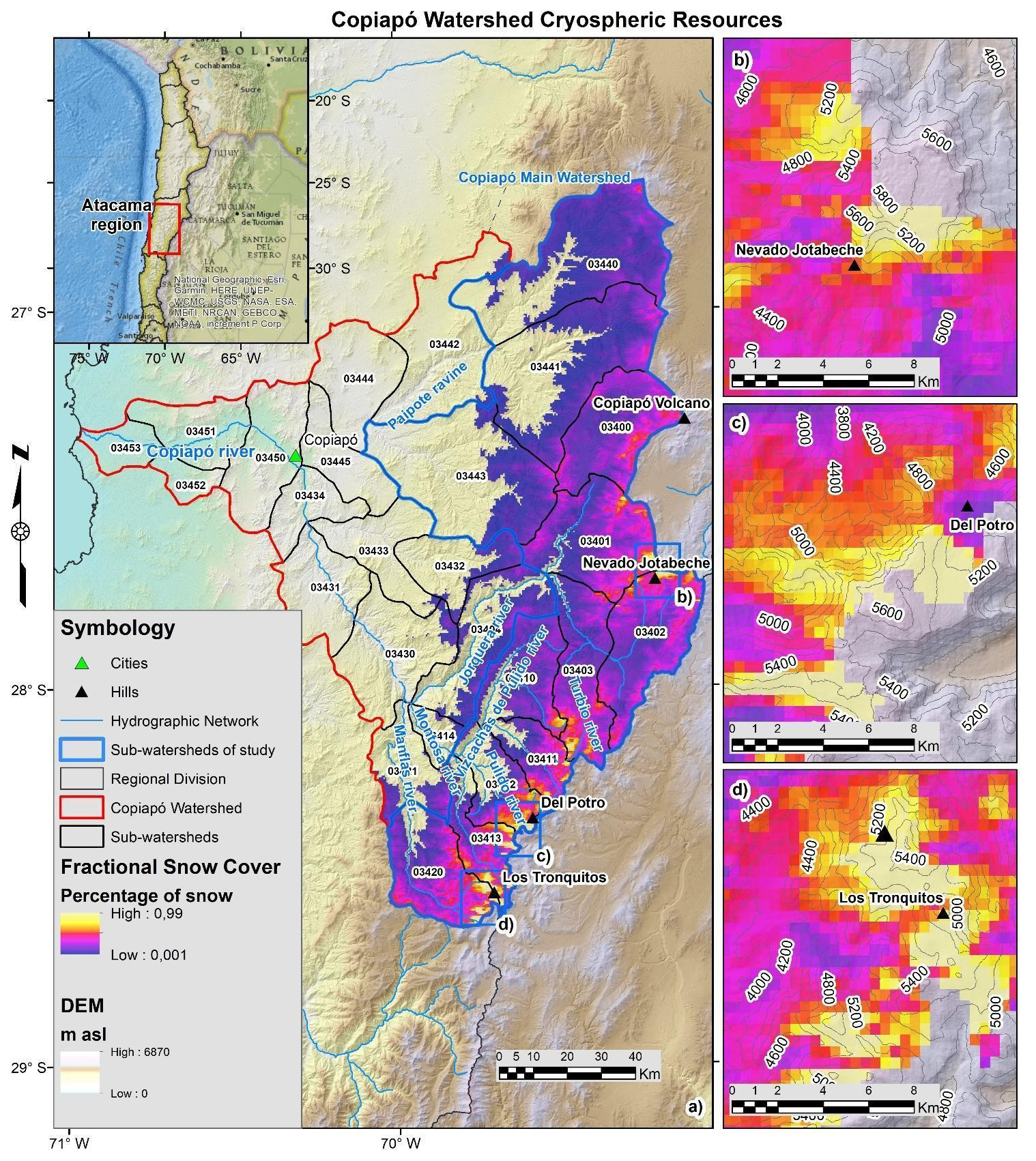
Figure 8 (a) Distribution map of the snow in the Copiapó watershed. (b) Jotabeche volcano snow permanence (c) The Potro hill snow permanence (d) The Tronquitos hill snow permanence. Basemap: Esri, Maxar, Earthstar Geographics, and the GIS User Community | Powered by Esri.

4.2 Analysis of runoff

Before incorporating snow permanence as a core variable of the NCI, we tested empirically whether MODIS-derived snow cover translates into a hydrological signal at the watershed scale. To do this, we contrasted streamflow behaviour during representative wet and dry years and quantified the statistical relationship between September snow extent and October–March mean discharge at the Copiapó River at Pastillo gauging station. Daily mean streamflow records at the Copiapó River at Pastillo station (Fig. 9) reveal distinct seasonal patterns between wet and dry years. During the wet year (October 2017–March 2018), streamflow exhibits a sustained increase from October to December, peaking at 5.7 m³ s⁻¹ in December, followed by a gradual decline through January and a secondary pulse in February (5.3 m³ s⁻¹). In contrast, the dry year (October 2013–March 2014) shows substantially lower spring flows, with mean streamflow averaging only 1.0 m³ s⁻¹ during October-November, and the most significant increases concentrated in December (1.3 m³ s⁻¹) and February (2.2 m³ s⁻¹). Overall, the wet year delivered 3.4 times more water than the dry year, with the greatest relative differences occurring in November (+471 %) and December (+343 %).

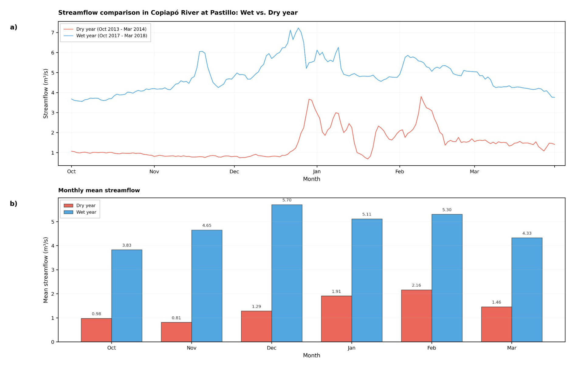
Figure 9 Daily (a) and monthly mean (b) streamflow at Copiapó River at Pastillo for wet (2017–2018, blue) and dry (2013–2014, red) years. Data Source: Dirección General de Aguas, Chile.

These contrasting patterns between individual years reflect broader interannual variability in snowpack accumulation, ice bodies and melt dynamics. To quantify this relationship at the watershed scale, we incorporated a new analysis linking MODIS-derived snow permanence in September, at the onset of the melt season, with mean river discharge observed between October and March (Fig. 10). This relationship shows a robust correlation (R²=0.58; r=0.76; N=22), confirming that seasonal snow permanence acts as a dominant short-term cryospheric water resource in the Copiapó watershed. The regression intercept (0.55 m³ s⁻¹) represents the melt-season discharge sustained independently of the current year’s snow, i.e. by longer-residence cryospheric storage. Its ratio to the observed discharge of each year, which ranges from 0.08 (2017–18) to 0.90 with a mean of 0.43 (0.27 and 0.62 for the wettest and driest tercile of snow years, respectively), is adopted as the ice weighting factor w of the NCI (Sect. 3.6; Fig. 19). However, the unexplained variance (42 %) suggests that other cryospheric components, such as rock glaciers, debris-covered ice, and possibly permafrost, may contribute to streamflow, particularly during low-snow years or late in the melt season when these longer-residence-time ice storage become more significant. The integration of these empirical hydrological results into the NCI framework validates that sub-watersheds with higher NCI values not only exhibit stronger cryospheric signatures in their topography but also display measurable hydrological responses consistent with multiple meltwater sources operating at different temporal scales.

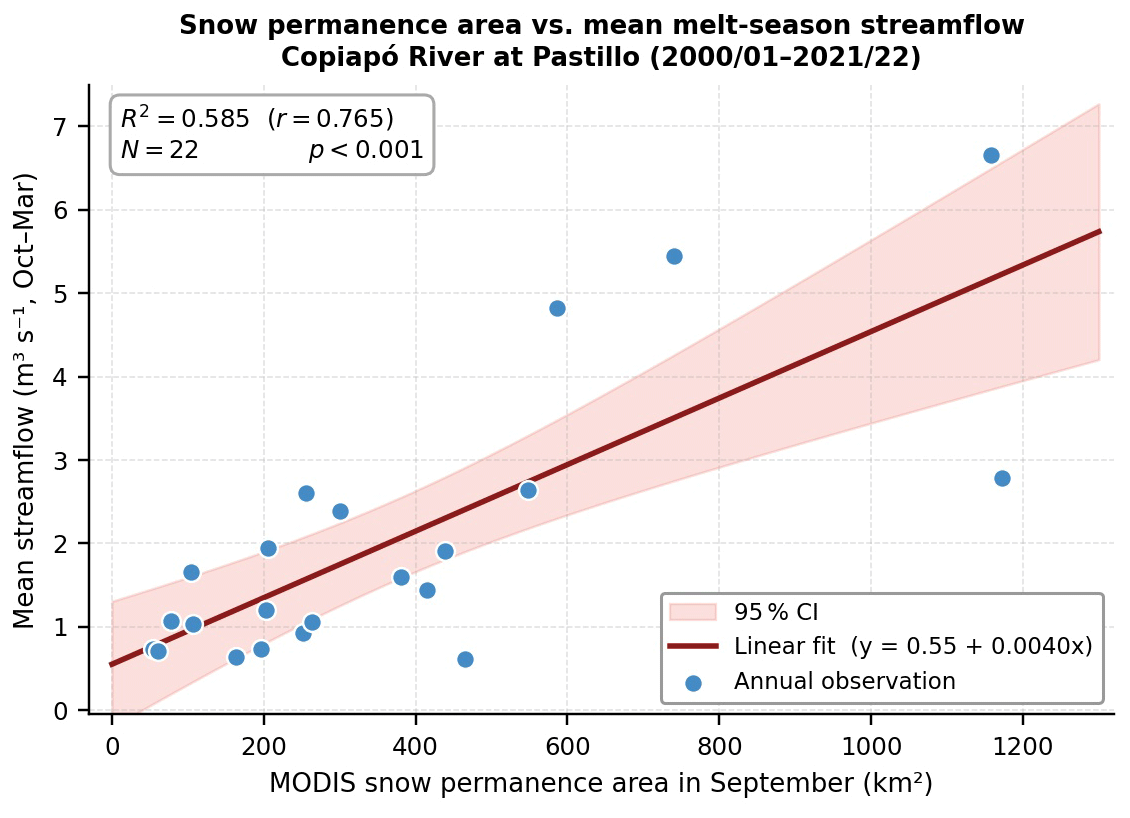
Figure 10 September snow-covered area vs. October–March mean discharge at Copiapó River at Pastillo (2000–2021, N=22). Linear regression (red line) with 95 % confidence interval (shaded). R²=0.58; r=0.76; p<0.001. Sources: MODIS MOD10A1 and DGA, Chile.

4.3 Field survey observations of cryospheric landforms

The fieldwork has yielded observations of cryospheric landforms in the Del Potro and Montosa River sub-watersheds (Figs. 11 and 12). The Del Potro Glacier (Fig. 12d) and the surrounding periglacial environment of the Del Potro river sub-watershed (03412; Fig. 11) were clearly identified during field surveys. In the Montosa River sub-watershed, the Maranceles Glacier (Fig. 12c) was also observed. Additional field observations confirmed the presence of well-developed rock glaciers, gelifluction taluses, and protalus lobes in the Del Potro river watershed (03412) (Fig. 11c–g).

Glacial landforms are preferentially distributed on south-facing slopes, as indicated by their aspect, which are generally associated with reduced incoming solar radiation. In contrast, periglacial cryospheric landforms such as protalus lobes and gelifluction taluses are more frequently found on exposed slopes with steeper gradients and variable aspects, reflecting differences in topographic setting rather than direct measurements of snow accumulation or thermal conditions. Debris-free and debris-covered glaciers are primarily located in topographic depressions and high-elevation headwaters. In contrast, protalus lobes and gelifluction taluses are predominantly distributed on steep slopes and debris-covered sectors. Overall, periglacial cryospheric landforms display a wider spatial distribution across the watershed than glaciers.

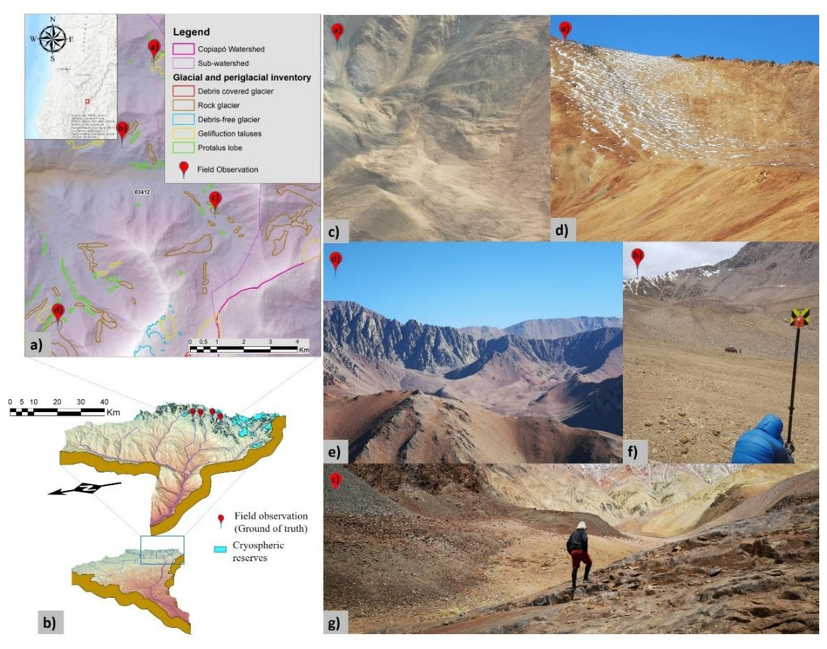
Figure 11 Field observations of cryospheric landforms as the ground truthing. (a) Map of cryospheric landforms distribution, (b) 3D view of the watershed, (c) Rock glacier of the Del Potro River (03412); (d) Gelifluction taluses of the Del Potro River (03412); (e) Rock glacier of the Del Potro River (03412); (f) Rock glacier of the Del Potro River (03412); (g) Panorama of different periglacial cryospheric landforms of the Del Potro River (03412). Basemap: Esri, Maxar, Earthstar Geographics, and the GIS User Community | Powered by Esri.

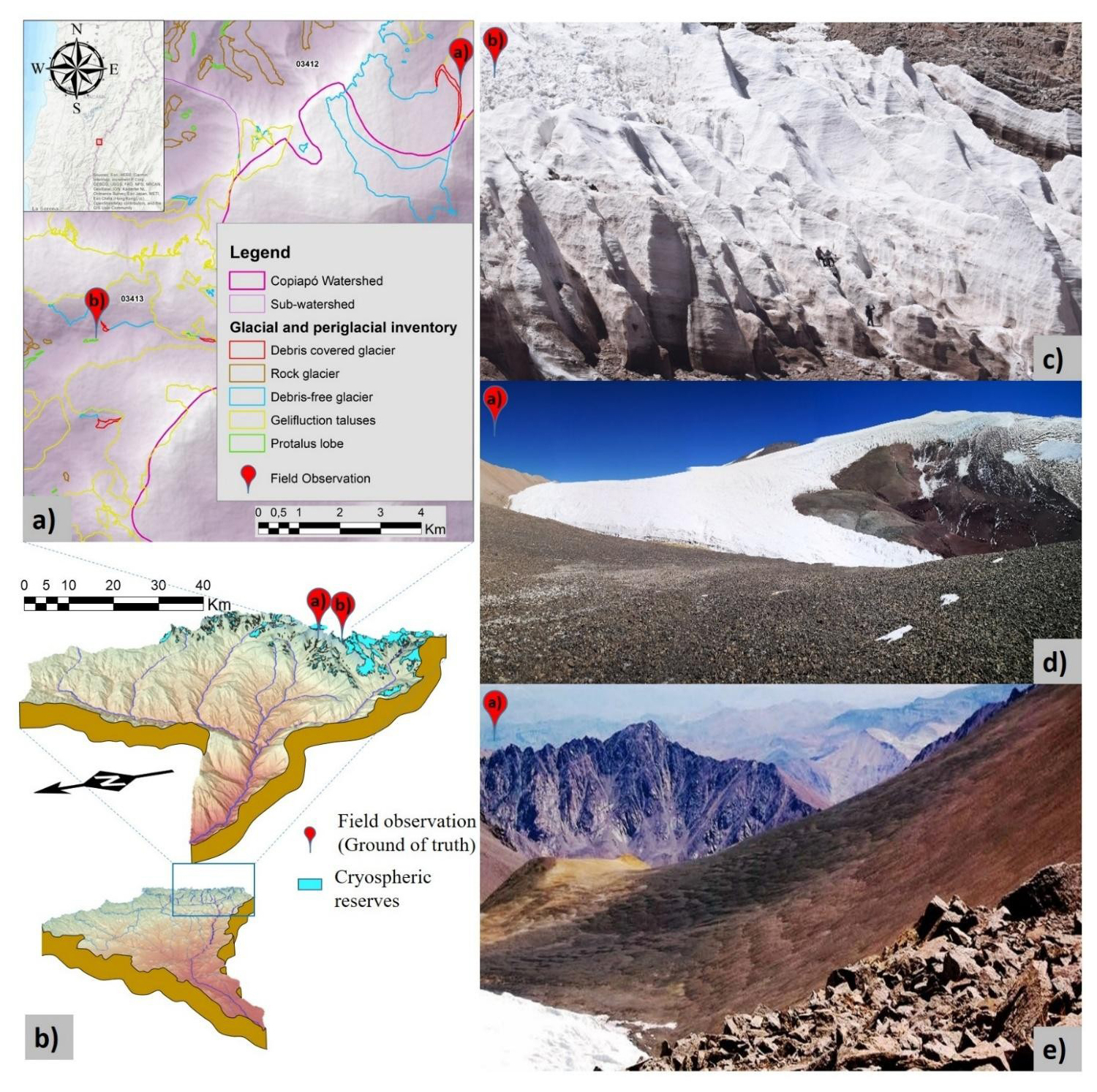
Figure 12 Field observations of cryospheric landforms as the ground truthing. (a) Map of cryospheric landforms distribution, (b) 3D view of the watershed, (c) Del Potro debris-free glacier of the Del Potro River (03412), (d) Maranceles glacier of the Montosa River (03413), (e) Gelifluction taluses of the periglacial environment of the Del Potro River (03412). Basemap: Esri, Maxar, Earthstar Geographics, and the GIS User Community | Powered by Esri.

4.4 Geophysical results

4.4.1 Gelifluction Taluses

Electrical resistivity tomography (ERT) results (Fig. 13) provides the basis for interpreting the internal structure of the gelifluction taluses. The lobate surface morphology characteristic of this cryospheric landform (Fig. 5a, b), together with the location and orientation of the tomographic profile (Fig. 5c, d), is clearly reflected in the geophysical response. The ERT profile extends over 295 m and crosses a sector of the landform displaying a well-developed pattern of freeze–thaw-related lobulations, starting at 4430 m a.s.l. in the upstream sector of the Montosa sub-watershed. This geomorphological pattern coincides with a high-resistivity zone (HRZ), with resistivity values ranging from approximately 1000 to 8000 Ωm. According to comprehensive reviews and field studies on mountain permafrost, such resistivity values are typical of ice-rich frozen ground, where pore water is largely transformed into electrically resistive ice (Hauck and Kneisel, 2008). Electrical resistivity is known to increase by several orders of magnitude upon freezing, particularly in coarse-grained periglacial materials, making ERT a robust tool for detecting ice-bearing permafrost bodies.

The HRZ delineates an ice-rich permafrost body with an estimated two-dimensional horizontal extension of approximately 20 m² within the tomographic section. Comparable resistivity ranges and internal structures have been documented in ice-rich permafrost landforms investigated with ERT, including rock glaciers, talus slopes and other periglacial slope systems (Kneisel et al., 2008; Hilbich et al., 2009). The association between lobate slope morphology and underlying frozen ground with significant ice content is consistent with the established understanding of gelifluction as a process operating on seasonally thawed active layers overlying permafrost, where ice lenses and frozen substrates exert a first-order control on deformation patterns (Matsuoka, 2001).

Downstream of 4430 m a.s.l., the HRZ terminates abruptly at the frontal sector of the last lobulations. From this point, a low-resistivity zone (LRZ) dominates, with resistivity values between 50 and 200 Ωm. This sharp contrast is interpreted as the transition from frozen ground to unfrozen, water-saturated sediments. Similar resistivity ranges have been reported for unfrozen debris, taliks and shallow groundwater zones underlying permafrost terrain, where electrolytic conduction through liquid water strongly reduces bulk resistivity (Hauck and Kneisel, 2008).

The spatial juxtaposition of the HRZ and LRZ suggests a direct subsurface connection between the ice-rich permafrost body and an underlying groundwater system. Studies combining ERT and seismic methods demonstrate that such resistivity contrasts commonly mark permafrost boundaries and zones of hydrological interaction, where water infiltration and ice loss can be detected geophysically (Hauck et al., 2008; Mewes et al., 2017). In particular, combined geophysical monitoring has shown that increases in liquid water content beneath or adjacent to frozen ground produce a pronounced decrease in resistivity, even when ice loss is spatially limited. Based on the vertical extent of the HRZ, the ERT data allow for the estimation of an average ice-rich core thickness of approximately 15 m (Fig. 13). This thickness falls within the range reported for ice-bearing periglacial slope landforms investigated using geophysical methods, where frozen layers commonly extend several tens of meters below the surface depending on material properties and thermal conditions (Kneisel et al., 2008; Hauck and Kneisel, 2008).

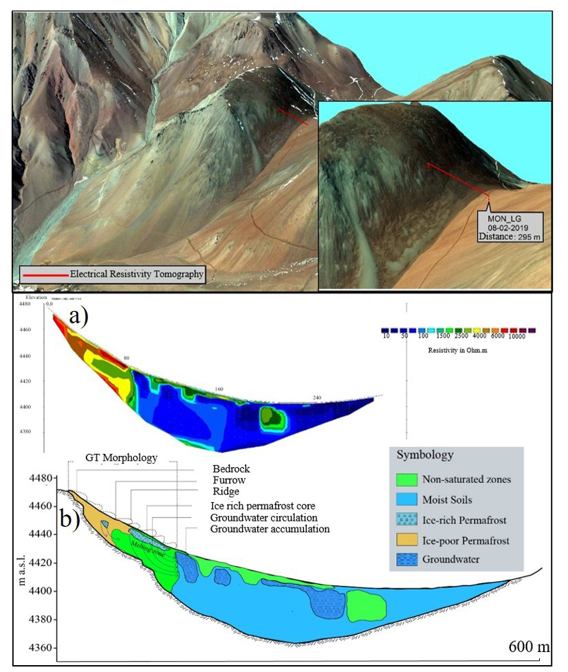
Figure 13 Results of the electrical resistivity tomography (ERT) over the gelifluction taluses cryospheric landforms in the Montosa Sub-watershed. (a) Electrical resistivity tomography, (b) Subsurface interpretation of resistivity test. Basemap: Esri, Maxar, Earthstar Geographics, and the GIS User Community | Powered by Esri.

4.4.2 Rock Glacier

A second ERT survey was conducted across a representative active rock glacier in the Montosa sub-watershed (Fig. 14). The tomographic sections reveal a complex internal structure characterized by laterally continuous high-resistivity zones (HRZ), which are interpreted as ice-rich permafrost bodies embedded within a coarse debris matrix, a configuration commonly reported for active rock glaciers worldwide (Kneisel et al., 2008).

Resistivity values exceeding approximately 4–10 kΩ ⋅ m dominate the central and frontal sectors of the landform, indicating the presence of massive or highly ice-saturated material. Comparable resistivity ranges have been documented in ice-rich rock glaciers in the Andes and other high-mountain regions, where electrical resistivity contrasts are primarily controlled by ground-ice content rather than lithological variability (Kneisel et al., 2008; Pavoni et al., 2021). These high-resistivity anomalies are spatially coherent with the surface morphology of the rock glacier, including its lobate structure and well-defined frontal slope, supporting a close correspondence between geomorphological expression and subsurface ice distribution.

Beneath the HRZ, lower-resistivity zones (LRZ; <1–5 kΩ ⋅ m) are observed, which are interpreted as unfrozen or partially saturated debris layers and/or underlying bedrock. The relatively sharp transition between high- and low-resistivity domains suggests a distinct boundary between ice-rich permafrost and unfrozen substrate, a feature widely reported in ERT studies of active rock glaciers (Kneisel et al., 2008).

The ERT-derived geometry indicates an average ice-rich layer thickness on the order of 20–30 m, with local maxima exceeding 35 m in the central part of the rock glacier body. These thicknesses fall within the range reported for active rock glaciers in the dry Andes based on geophysical surveys and regional assessments (Brenning, 2005; Azócar and Brenning, 2010; Halla et al., 2021). The observed thickness values provide an independent observational constraint for the thickness estimates derived from the viscoplastic creep inversion (Cicoira et al., 2021) based on DInSAR surface velocities.

Importantly, the spatial extent of the HRZ aligns closely with the mapped rock glacier polygon, reinforcing the validity of the inventory-based delineation and confirming that the geophysically detected ice body corresponds to the geomorphological unit considered in the volume calculations. The ERT results therefore serve as ground-based validation for both the presence of ice-rich permafrost and the order of magnitude of the modeled thicknesses applied to rock glaciers within the Copiapó watershed, consistent with previous multi-method approaches combining geomorphology, geophysics, and kinematic observations.

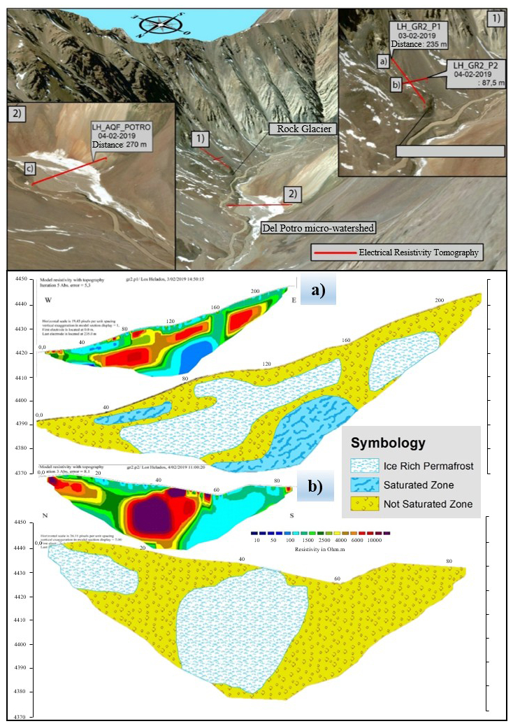
Figure 14 Results of the electrical resistivity tomography (ERT) over rock glacier cryospheric landforms in the Del Potro Sub-watershed, (a) Longitudinal tomography, (b) Cross-sectional tomography. Basemap: Esri, Maxar, Earthstar Geographics, and the GIS User Community | Powered by Esri.

4.5 Thickness estimations on periglacial landforms

Surface displacement maps (Fig. 15) of a representative rock glacier in the Copiapó watershed show a coherent downslope motion that is clearly confined to the rock glacier body, while surrounding terrain remains stable, supporting the reliability of both the cryosphere inventory and the DInSAR processing. These surface velocities provide a direct kinematic constraint for the viscoplastic thickness modelling of ice-rich permafrost landforms used in this study.

The modeled ice-rich layer thicknesses for the main periglacial cryospheric landforms (rock glaciers, protalus lobes, and gelifluction taluses) and their relationship with DInSAR-derived surface velocities (Fig. 16) show that rock glaciers exhibit the largest modeled thicknesses, with median values on the order of ∼ 25–30 m and a wide interquartile range, reflecting both their higher surface velocities and the greater mechanical efficiency of creep in these landforms. In contrast, protalus lobes show intermediate thicknesses, typically below ∼ 15 m, while gelifluction taluses are characterized by consistently thinner ice-rich layers, generally <10 m. The scatter plot highlights a positive relationship between mean surface velocity and modeled thickness across all periglacial cryospheric landforms, consistent with the viscoplastic framework in which higher deformation rates require larger ice thicknesses to sustain basal shear stress under comparable slope conditions.

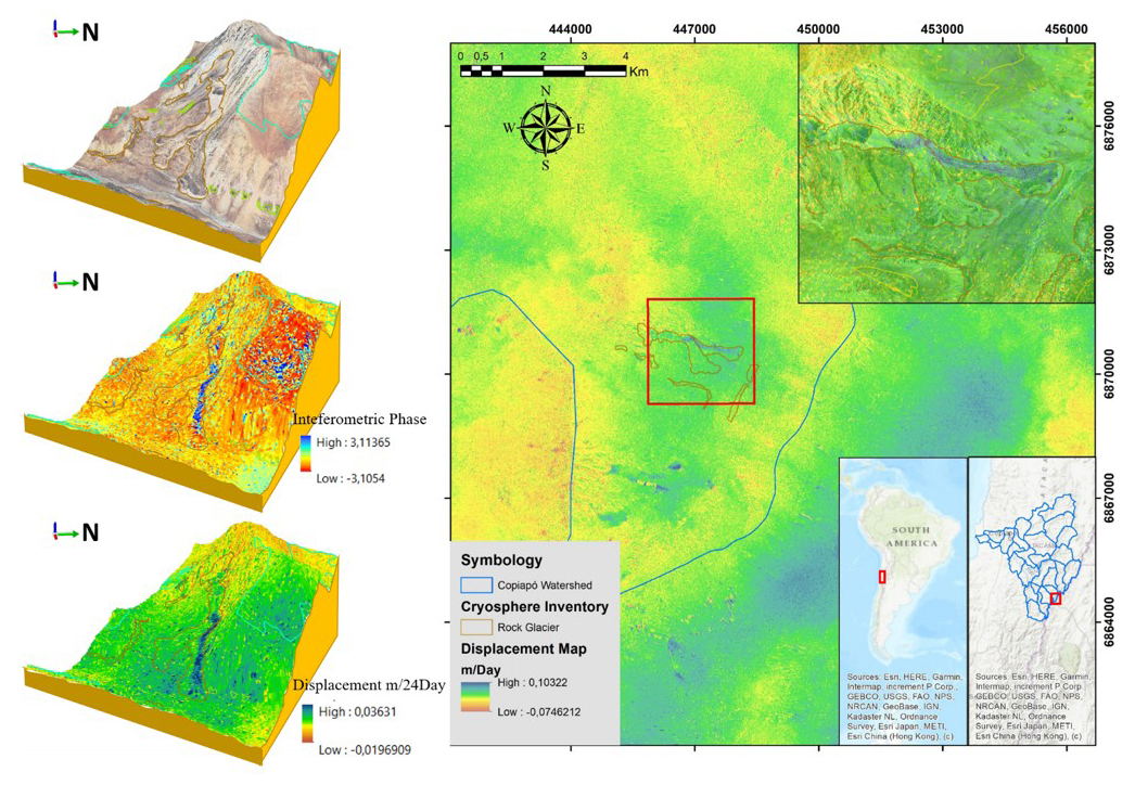
Figure 15 Example of DInSAR-derived surface displacement of a rock glacier in the Copiapó Watershed. Basemap: Esri, Maxar, Earthstar Geographics, and the GIS User Community | Powered by Esri.

Rock glaciers cluster at higher velocities and thicknesses, whereas protalus lobes and gelifluction taluses occupy lower-velocity regimes, with substantial overlap reflecting variability in slope, thermal state, and internal ice content. Despite this overlap, the three cryospheric landforms groups remain clearly distinguishable in thickness–velocity space, supporting the application of a unified viscoplastic model while preserving cryospheric landforms-specific structural differences. These results confirm that surface kinematics derived from DInSAR provide a physically meaningful constraint on subsurface ice thickness and justify their use for estimating ice volumes in ice-rich permafrost landforms across the Copiapó watershed. These thickness estimates are further contextualized by multi-decadal kinematic records from the Dry Andes showing that rock glaciers exhibit marked interannual velocity variability (Vivero et al., 2021), and by debris-covered glacier studies demonstrating that supraglacial debris exerts a strong control on the hydrological behavior of ice bodies in high-elevation Andean catchments (Burger et al., 2019). The long-term hydrological relevance of these landforms is reinforced by projections indicating reduced glacier meltwater contributions under future megadrought scenarios (Ayala et al., 2025), which elevate the importance of accurately quantifying periglacial ice reserves such as those estimated here.

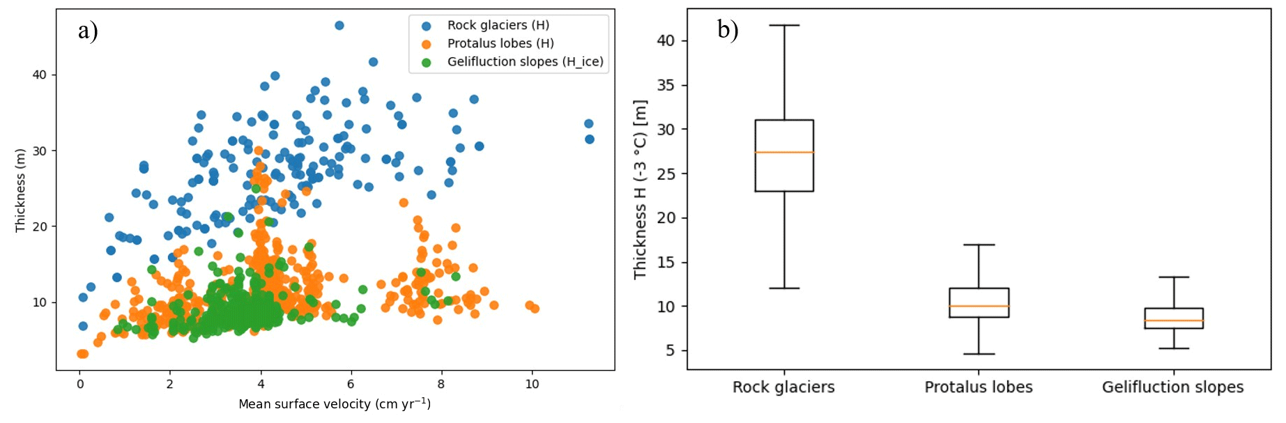
Figure 16 Modeled thickness–velocity relationship for periglacial cryospheric landforms of Copiapó Watershed.

4.6 Ice volumes, snow area and NCI for sub-watershed

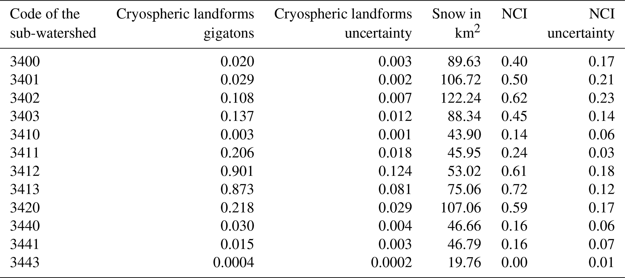
The ice volumes, snow area and the NCI for each of the sub-watersheds that constitute the cryospheric landforms of the Copiapó River watershed have been calculated (Table 6). The watershed with the largest ice masses is the Del Potro River watershed (03412), with 0.901 Gt, followed by the Montosa River watershed (03413) with 0.873 Gt and thirdly the southernmost watershed, the Manflas River watershed (03420) with 0.218 Gt of ice. In terms of volume, the largest ice volumes in the entire watershed are found in debris-free glaciers, gelifluction taluses and rock glaciers (Fig. 17).

Following the mapping of snow, we observe that the surface area distribution of snow cover is uneven, with a higher density in the southern part and the northern end of the watershed. In the south, the watersheds with the largest snow permanence are the Manflas River (03420), with 107.06 km² of mean snow cover (2000–2024), the Montosa River (03413) with 75.06 km² and the Del Potro River (03412) with 53 km². In the north, the most important rivers are the Estero Come Caballos (03402) with 122.24 km², Figueroa River (03401) with 106.72 km², Quebrada Monardes (03400) with 89.63 km² and the Cachitos River (03403) with 88.34 km² (Table 6).

Figure 17 Total ice mass of the Copiapó Watershed.

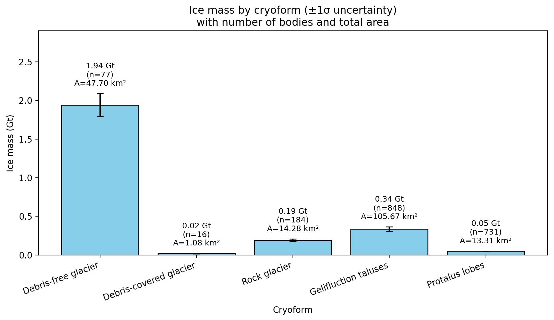
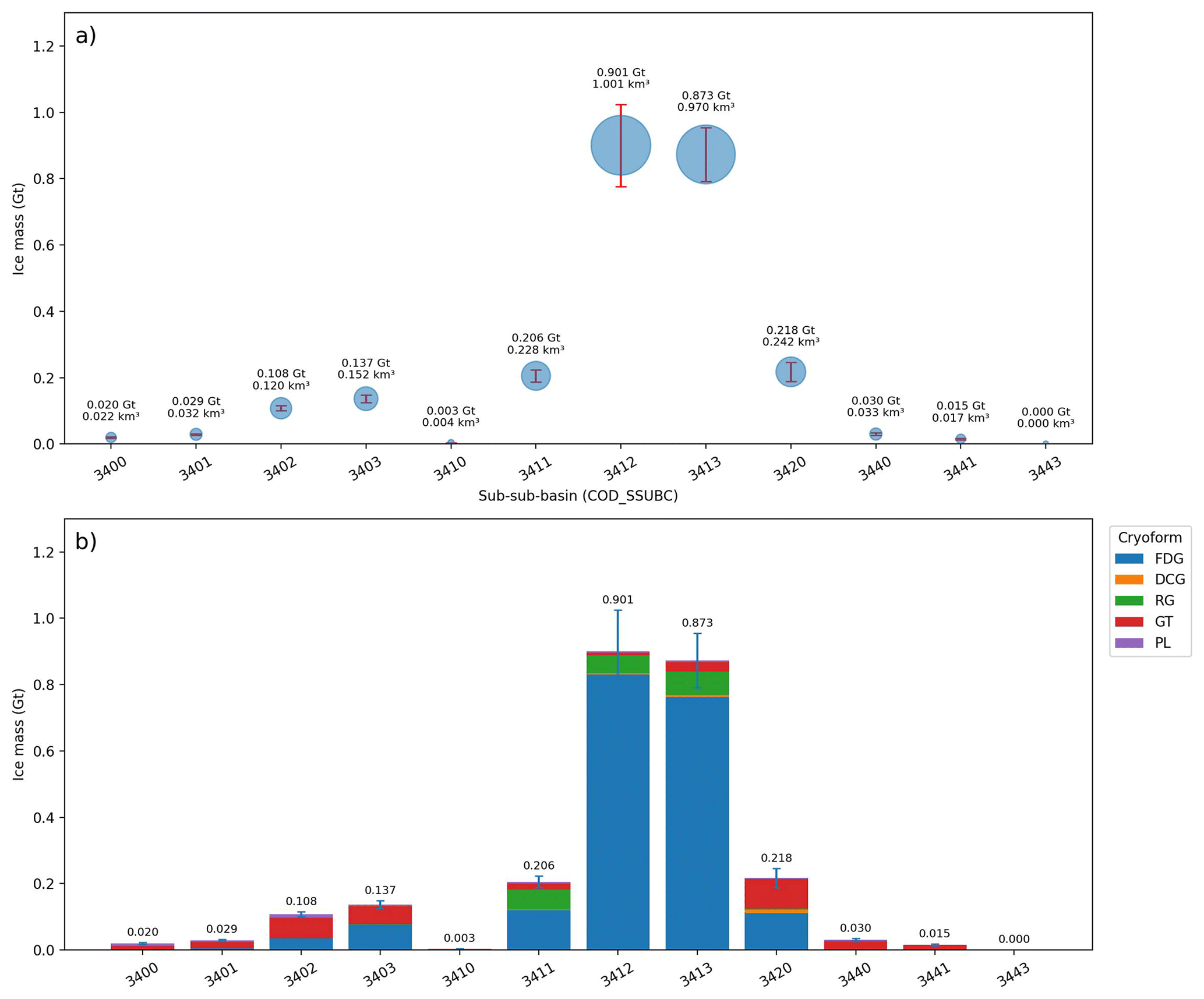
Figure 18 Total ice volumes of the Copiapó Watershed expressed both as (a) total ice mass with associated uncertainty and (b) as stacked contributions by cryospheric landforms.

The distribution of ice mass across cryospheric sub-watersheds of the Copiapó watershed (Fig. 18), reveal a highly heterogeneous spatial distribution of cryospheric landforms, with a small number of sub-watersheds concentrating the majority of the total ice mass.

The largest ice masses are found in the Montosa (COD_SSUBC 3413) and Del Potro (3412) sub-watersheds, each storing approximately ∼ 0.9 Gt of ice. These watersheds clearly dominate the cryospheric landforms of the watershed and are characterized by the combined presence of debris-free glaciers, rock glaciers, and extensive ice-rich permafrost landforms. In contrast, several sub-watersheds exhibit ice masses below 0.1 Gt, reflecting either limited cryospheric landforms extent or the dominance of thin periglacial landforms.

The stacked representation highlights that debris-free glaciers constitute the principal contribution to ice mass in the largest ice storage, whereas ice-rich permafrost cryospheric landforms, particularly rock glaciers and gelifluction taluses, represent a substantial fraction of the total ice mass in intermediate and smaller sub-watersheds. Protalus lobes contribute minor but non-negligible volumes in selected sub-watersheds, emphasizing their cumulative importance at the watershed scale.

Uncertainty ranges are largest in sub-watersheds dominated by periglacial cryospheric landforms, reflecting the combined effects of variability in surface velocity, thermal state, ice content, and mapped area. Nevertheless, the relative ranking of sub-watersheds by total ice mass remains robust, with Montosa and Del Potro consistently emerging as the primary cryospheric landforms within the Copiapó watershed.

Overall, these results demonstrate that cryospheric ice mass is strongly concentrated in a limited number of sub-watersheds, while many others contain comparatively small but non-negligible ice volumes distributed among different cryospheric landforms. However, ice mass alone does not fully capture the hydrological relevance of a watershed, as it does not account for the capacity to regenerate water resources through snowfall. This motivates the integration of cryospheric landforms (ice mass) and snow (Permanence) into a unified metric, introduced in the following section as the Normalized Cryospheric Index (NCI).

The Normalized Cryospheric Index (NCI) behavior in relation to the relative weighting of ice volume (V) and snow occurrence (S), along with the stability of sub-watershed rankings under uncertainty (Fig. 19) shows how the choice of weight (w) influences the mean value of the NCI and, ultimately, the final ranking of the sub-watersheds.

The evolution of the mean NCI value of each sub-watershed as w varies from zero to one (Fig. 19a). Each line represents a different sub-watershed, so that the slopes and crosses between lines allow us to appreciate which sub-watershed are favored by a greater relevance of ice volume V (when w tends to 1) or snow cover S (when w tends to 0). This preliminary behavior shows, on the one hand, the sensitivity of each subwatershed to weighting and, on the other hand, the possible dominance of one variable over the other in certain w zones.

The position in the ranking that each subwatershed occupies for each w value (Fig. 19b) shows that the horizontal lines extend from the first position (1) to the last. It highlights consistently privileged-ranked subwatersheds regardless of w, in contrast to unstably ranked subwatersheds. This early insight into the stability of the ranking compellingly underscores the urgency of undertaking a rigorous robustness analysis.

The ranking variability function, defined as the sum (or average) of the standard deviations of the position of each sub-watershed in the different simulations (Fig. 19c) quantifies the overall stability of the ranking for each w. The function decreases steadily from the snow-dominated (w≈0.2) towards the ice-dominated (w≈0.9) end, indicating that the ranking becomes less sensitive to data uncertainty as more weight is given to ice mass, whose differences between sub-watersheds are larger relative to their uncertainty than those of snow. Within the hydrologically observed range of w (vertical lines in Fig. 19c: 0.27 in wet years, 0.43 on average and 0.62 in dry years), the function drops from about 11 to 6, i.e. the dry-year ranking is roughly twice as stable as the wet-year ranking.

The mean NCI (with its error bars) for each watershed obtained by sampling w from its observed 2001–2022 distribution in each Monte Carlo replicate (mean w=0.43; Fig. 19d) shows that the vertical axis reflects the average magnitude of the index, while the error bars indicate the standard deviation derived from the Monte Carlo simulations. Thus, the visualization offers a clear identification of the watersheds with the highest NCI values, while simultaneously exposing the degree of uncertainty surrounding these estimates. The error bars therefore include both data uncertainty and the variability of the hydrological regime, and provide a detailed view of the dispersion of each watershed.

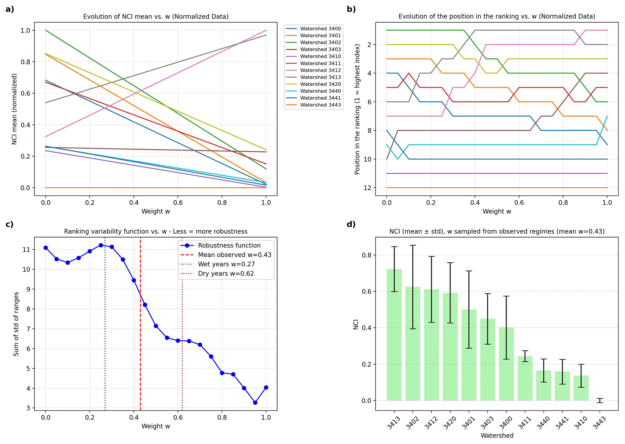
Figure 19 Analysis of NCI and robustness of the ranking as a function of w weighting (a) Evolution of the mean NCI for each sub-watershed as w varies between 0 and 1 (b) Position in the ranking of each sub-watershed as a function of w (c) Ranking variability function (sum of the standard deviations of the positions), with vertical lines marking the observed mean w (0.43) and the wet-year (0.27) and dry-year (0.62) values (d) Mean NCI ± standard deviation with w sampled from its observed 2001–2022 distribution, evidencing the magnitude and dispersion of the index in each sub-watershed.

The calculated NCI, demonstrated that the sub-watershed with the highest NCI was the Montosa River watershed (03413) (NCI = 0.72 ± 0.12), followed by the Estero Come Caballos watershed (03402) (NCI = 0.62 ± 0.23), the Del Potro River watershed (03412) (NCI = 0.61 ± 0.18), the Manflas River watershed (03420) (NCI = 0.59 ± 0.17) and the Figueroa River watershed (03401) (NCI = 0.50 ± 0.21). The ranking depends on the hydrological regime: under dry-year conditions (w=0.62) Montosa and Del Potro occupy the first two positions in practically all simulations (probability of ranking among the top three ≈1.0), followed by Manflas (0.62), whereas under wet-year conditions (w=0.27) Estero Come Caballos (0.94), Manflas (0.80) and Montosa (0.69) lead the ranking and Del Potro falls to the sixth position. Montosa is thus the only sub-watershed that ranks among the top three under all regimes, Del Potro is the key reserve for dry years, and in the northern region the Estero Come Caballos sub-watershed is highlighted by the index in wet and average years, primarily attributed to its persistent snow cover.

Table 6 Summary of results by sub-watershed of cryospheric landforms in Gt, snow in km² and NCI index.

5 Discussion

5.1 Cryospheric landforms and snow permanence in the Copiapó watershed

From the cryospheric landforms and snow occurrence mapping exercises (Figs. 4 and 8), we observed that the cryospheric landforms of the Copiapó watershed are predominantly located at altitudes above 4500 m. This compares well with other regions in which snowfall has been identified to be controlled by altitude (Saydi and Ding, 2020). We also observed that cryospheric landforms occur in smaller, isolated regions (<0.25 km² in width) in the northern part of our research area. This corresponds with our own field observations, where most cryospheric landforms occur in smaller bodies (Fig. 4). This resulted in smaller, separated cryospheric landforms and surrounding the highest point (Fig. 4b and c). They host smaller cryospheric landforms, for example near the Cadillal and the Nevado Jotabeche, compared to the southern part of our study area. Because those northern cryospheric landforms are located in or in proximity of the SAAD (Abraham et al., 2020), snowfall and permanent snow occurrences are limited, leading to isolated cryospheric landforms (Fig. 4). The potential volume of water that is captured in cryospheric landforms in the sub-watersheds of the Copiapó watershed (Fig. 1) is thus strongly influenced by the South American Arid Diagonal (SAAD) that controls the distribution of the different types of cryospheric landforms (García et al., 2017). In our case, the proximity of the Copiapó watershed to the SAAD limits the occurrence of debris-free glaciers in the watershed north of 28.1° S latitude and limits the continuity of the cryosphere that is mainly attributed to cryospheric landforms associated with ice-rich permafrost, such as small rock glaciers, protalus lobes and predominantly gelifluction taluses.

In the more central domain in between Cadillal and Caserones no cryospheric landforms occur. This can be explained by the mechanical forcing of the South American low-level jet and the topographic blocking of the Andes (Insel et al., 2009). In the central sector, Mount Pissis exhibits greater elevation on the Argentinian side. Consequently, the prevailing northeasterly winds transporting moisture from the Pacific Ocean are obstructed by the Argentine portion of the mountain. This orographic interception results in localized snowfall on its Argentinian slopes, rather than allowing precipitation to be deflected by the comparatively lower-elevation Chilean topography. The topography north of Cadillal and south of Caserones is high enough to block these winds on the Chilean side, leading to snowfall and eventual cryospheric landforms in the southern regions in our research area. A last negative spatial correlation between the snowfall and the cryospheric landforms is the large snowfall anomaly in the northern area. The permanent snow occurrence is high, while not many cryospheric landforms are produced. The reason for this is the location of this region in the SAAD, resulting in melting or sublimation of the snow that does arrive in this area (Réveillet et al., 2020), meaning that the snow does not end up in cryospheric landforms.

From the different cryospheric landforms, we see that gelifluction taluses cover the largest surface area in the Copiapó watershed compared to other cryospheric landforms in our research areas (García et al., 2017). Field observations also confirm that gelifluction taluses extend across significantly broader areas compared to other cryospheric landforms (Fig. 12). The limited understanding of gelifluction taluses has led to their exclusion from global cryospheric reserve inventories. Nevertheless, in assessing watershed ice volume, these taluses emerge as the second most important ice store after debris-free glaciers (0.34 Gt), surpassing rock glaciers and protalus lobes (Fig. 17). Furthermore, the ERT-derived thickness measurements across the gelifluction lobe reveal a minimum detectable thickness of 15 m, which markedly contrasts with the range of 1 to 5 m reported by Hilbich et al. (2022).

On a more regional scale, we observe that in the south of the watershed, debris-free glaciers are always in contact with gelifluction taluses. This is confirmed in the field (Fig. 12). In the north of the Copiapó watershed, gelifluction taluses occur more as isolated bodies. The topography of the northern area is controlled by Tertiary volcanoes (Kay et al., 1994). In general, these volcanoes exhibit gentler slopes than those of the Principal Cordillera (Harrington, 1961) and largely shape the topography of our southern research area. Given that gelifluction taluses require steep slopes to form (Fig. 2), they are more likely to develop in the southern sector, where the terrain is dominated by the steep relief of the Principal Cordillera unlike in the north, where this feature is absent. Moreover, in the Central Cordillera glacial cirques are abundantly present (Evans, 2006). Glacial cirques provide sheltered environments that shield snow from extreme weather conditions, facilitating its recrystallization into exposed glaciers and other cryospheric landforms. The distribution of rock glaciers and protalus lobes is likewise influenced by the presence of glacial cirques (Palacios et al., 2020), resulting in their predominant occurrence in the southern portion of our study area. In contrast, no exposed glaciers are found north of Copiapó Hill (Fig. 4). Instead, gelifluction taluses and protalus lobes allow the continuity of the cryospheric fringe of the watershed. The absence of debris-free glaciers in this region is directly related to the South American low-level jet and the topographic blocking of the Andes (Insel et al., 2009).

These DGA (2014) volumes were used to provide a magnitude check. At the Del Potro Glacier, the modeled volume is ∼ 24 % larger than the GPR-based estimate; at the Tronquitos Glacier, the difference is larger (∼ 70 %). This spread is within the expected uncertainty range for individual glacier inversion products in Farinotti et al. (2019), particularly for small glaciers with limited thickness constraints. The DInSAR-derived surface velocities of rock glaciers in the Copiapó watershed are systematically lower than those reported for rock glaciers at comparable elevations further south in the Dry Andes. Vivero et al. (2021) documented mean surface velocities of 0.26 m yr⁻¹ during 1956–1978 and up to 1.25–1.80 m yr⁻¹ during 2014–2019 for the Tapado, Las Tolas, and El Cachito rock glaciers at 30° S in the Coquimbo Region. In contrast, the rock glaciers of the Copiapó watershed (26°41^′–28°24^′ S), as detected by Sentinel-1 DInSAR, exhibit velocities on the order of a few millimetres per year, one to two orders of magnitude slower. Two complementary factors explain this systematic difference. First, the Copiapó watershed lies within or immediately adjacent to the South American Arid Diagonal (SAAD), where extremely limited precipitation results in drier, colder permafrost conditions and reduced ground-ice temperatures relative to sites further south. Lower permafrost temperatures translate directly into higher ice viscosity and reduced creep rates under equivalent basal shear stresses, consistent with the strong temperature dependence of the Glen-type flow law applied in this study (Cicoira et al., 2021; Koenig et al., 2025). Second, the cryospheric landform genesis differs fundamentally between the two sites. The Tapado complex studied by Vivero et al. (2021) comprises glacigenic rock glaciers, landforms that originated from or remain connected to glacier ice and push moraines, and which therefore tend to be ice-richer and more dynamically active. The rock glaciers inventoried in the Copiapó watershed are predominantly cryogenic in origin, having developed through progressive freezing of talus and debris-slope material under permafrost conditions, without a direct glacial ice source. Cryogenic rock glaciers characteristically exhibit lower ice contents, more heterogeneous debris-ice matrices, and slower creep rates than glacigenic forms (Monnier and Kinnard, 2015). The slower kinematics observed in the Copiapó watershed are therefore physically consistent with both the arid thermal regime imposed by proximity to the SAAD and the cryogenic origin of the inventoried rock glaciers, and do not reflect anomalous model behaviour in the viscoplastic thickness inversion.

The DGA (2014) GPR-derived ice volume estimates were used as an independent benchmark to evaluate the magnitude of the modeled glacier volumes (Table 7). For Del Potro Glacier, the modeled volume (0.362 km³) exceeds the GPR-based estimate (0.293 km³) by approximately 24 %. In the case of Tronquitos Glacier, the discrepancy is larger, with the modeled volume (0.157 km³) being about 70 % higher than the GPR-derived value (0.092 km³).

Despite these differences, the observed spread is consistent with the uncertainty ranges reported for individual glacier ice-thickness inversion products in Farinotti et al. (2019). This is particularly relevant for small glaciers, where limited field-based thickness constraints and complex geometries tend to amplify relative errors in volume estimates. Therefore, while the discrepancies, especially for Tronquitos, are non-negligible, they remain within the expected variability for regional-scale glacier volume modeling.

A relevant consideration regarding the ice volume estimates for debris-free glaciers in the Copiapó watershed concerns the difference in glacier area between the two inventories used. The regional inventory of García et al. (2017) maps a total of 1907 ha of uncovered glaciers within the Copiapó watershed, whereas the Randolph Glacier Inventory (RGI) v6.0, which forms the basis for the Farinotti et al. (2019) thickness product used in this study, encompasses a larger glacier area for the same watershed. Because the Farinotti et al. (2019) volumes are computed over the RGI glacier polygons, which are more extensive than those delineated by García et al. (2017), the total ice volume attributed to debris-free glaciers in this study may overestimate the volume that would be obtained if the García et al. (2017) glacier boundaries were used instead. This discrepancy arises from methodological differences in glacier delineation, inventory date, and mapping criteria between the two datasets, and represents an inherent source of uncertainty in the volume estimates reported here. Future work should aim to reconcile these inventories and assess the sensitivity of the modeled ice volumes to the choice of glacier outlines, particularly for small and fragmented glacier bodies in the northern sector of the watershed.

Table 7 Comparison between modeled glacier ice volumes from Farinotti et al. (2019) and GPR-derived ice volumes reported by DGA (2014) for Del Potro and Tronquitos glaciers.

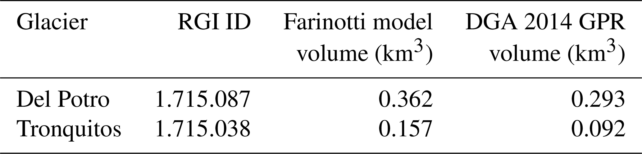
The watershed with the best balance between cryospheric landforms and snow permanence is the Montosa River watershed (03413) (Fig. 20), which contains high quantities of both cryospheric landforms and snow permanence. The field observations of geomorphological features that are indicative of active cryospheric landforms, such as the subparallel terraces (Fig. 12e), fit well with the mapped cryospheric landforms from our workflow. The mapped surface area and thickness are supported by the observed surface area and thickness in the field. Lastly, debris-covered glaciers occur predominantly in areas with a relatively continuous cryosphere (García et al., 2017). This is consistent with our findings that debris-covered glaciers are exclusively located in the southern region of the study area, a zone characterized by a more extensive and contiguous cryospheric distribution relative to the fragmented northern sectors. The interannual variability in glacier meltwater contribution in high-elevation Andean catchments is strongly modulated by the insulating effect of supraglacial debris, which attenuates ablation rates and delays the hydrological response of debris-covered glaciers relative to their clean-ice counterparts (Burger et al., 2019). Complementing this, multi-decadal monitoring using aerial and satellite photogrammetry and UAV surveys has demonstrated that rock glaciers in the Dry Andes exhibit significant kinematic variability, underscoring their dynamic role in the cryospheric system of the region (Vivero et al., 2021).

5.2 Classifying and prioritizing sub-watersheds in the Copiapó watershed

Unlike rainfall-dominated catchments, the upper Copiapó watershed is strongly influenced by cryospheric processes, with its headwaters characterized by the widespread presence of glaciers, rock glaciers, and ice-rich permafrost landforms. Cryospheric elements are concentrated in the high-altitude sub-watersheds, where water storage and seasonal runoff generation are controlled primarily by snow accumulation, snow persistence, and long-term ice storage rather than by direct rainfall inputs.

The Normalized Cryospheric Index (NCI) identifies three main sub-watersheds with a dominant cryospheric influence on the hydrological functioning of the Copiapó system, based on the combined contribution of ice mass and long-term snow persistence. The spatial distribution of cryospheric landforms shows a 97 % overlap with high-probability permafrost zones predicted by the global permafrost model of Gruber (2012), providing independent support for the relevance of ice-rich permafrost as a key component of water storage in the watershed. Together, these observations justify classifying the upper Copiapó as a cryosphere-influenced watershed, in which cryospheric processes exert a first-order control on water availability. The critical sub-watersheds include: the Montosa River (03413), Del Potro River (03412) and Manflas River (03420) (Table 6). Their spatial distribution corresponds to zones of maximum snow permanence and the most extensive cryospheric continuity within the Copiapó watershed (Figs. 6 and 8). These high indexes thus directly correlate with the cryospheric landforms and snowfall occurrences. For example, enhanced snowfall is concentrated in the Cerro del Potro sub-watershed (03412), where the largest debris-free glacier of the Copiapó watershed is located (Fig. 8c). This area hosts El Potro Glacier, the most extensive binational glacier in northern Chile (García et al., 2017), indicating a strong coupling between snow accumulation, glacier development, and long-term ice storage. As a result, the Cerro del Potro sub-watershed ranks among the highest NCI values, reflecting the combined importance of snow (permanence) and cryospheric landforms (ice mass). This combination has the potential to control the presence of water resources downstream when global temperatures continue to rise (Flores et al., 2018). Notably, recent projections for the Southern Andes indicate that glacier meltwater contributions may decline substantially during future megadrought conditions (Ayala et al., 2025), reinforcing the urgency of identifying and protecting cryospheric sub-watersheds such as those ranked highest by the NCI. With this study, we detected the sub-watersheds that should be prioritized. In wet years, snow controls the watershed hydrology in the northern part of the Copiapó watershed. This means that in these locations infrastructure needs to be put in place to capture the larger amounts of run-off that will arrive with increasing warmer temperatures, such as the Estero Come Caballos sub-watershed (03402), with the second place of the NCI. In times of water scarcity, we identified that the sub-watersheds of the Montosa River (03413), Del Potro River (03412), and Manflas River watershed (03420) will contribute most of the flow to the Copiapó River.

Given the observed relationship between snowfall and cryospheric landforms distribution, prioritizing the Copiapó watershed is essential to safeguard its water resources. We propose a systematic framework to evaluate and rank sub-watersheds according to preliminary assessments of cryospheric landforms and resource availability. From this ranking (Table 6), the main target, with the highest NCI is the sub-watershed of Montosa River (03413). The second and third targets for dry years are located towards the south, the Del Potro River (03412) and the Manflas River watershed (03420), and finally the last targets are Estero come Caballos (03402) and Figueroa River (03401) watersheds, which lead the ranking in wet years (Table 6). These five sub-watersheds constitute the basis for continuous water production in the Copiapó watershed during dry years, because they host 83.8 % of the cryospheric landforms ice volume of the Copiapó watershed. From these four sub-watersheds, the Montosa River watershed (03413) maintains the best balance between snow and cryospheric landforms (Fig. 20). We have shown that with this hydrological approach, the NCI allows us to infer that the sub-watershed with the highest hydrological importance is the Montosa River watershed (03413). This index also allowed us to observe that the watersheds of the northern region are high in snow cover but are less enriched in cryospheric landforms. During years of substantial snowfall, management efforts should prioritize northern sub-watersheds, such as the Estero Come Caballos Sub-watershed (03402). This suggests that northern watersheds exhibit a limited ability to develop cryogenic niches, as snow in these areas is primarily lost through melting or sublimation. A potential explanation for the lack of cryospheric landforms in northern watersheds lies in their geomorphological characteristics, which may hinder the accumulation and preservation of ice.

Based on the calculation of the NCI, we have been able to identify that the Estero Come Caballos watershed (03402) is the most strategic for snow accumulation, even surpassing the watersheds in the southern part of the Copiapó watershed in terms of snow permanence (Fig. 20).

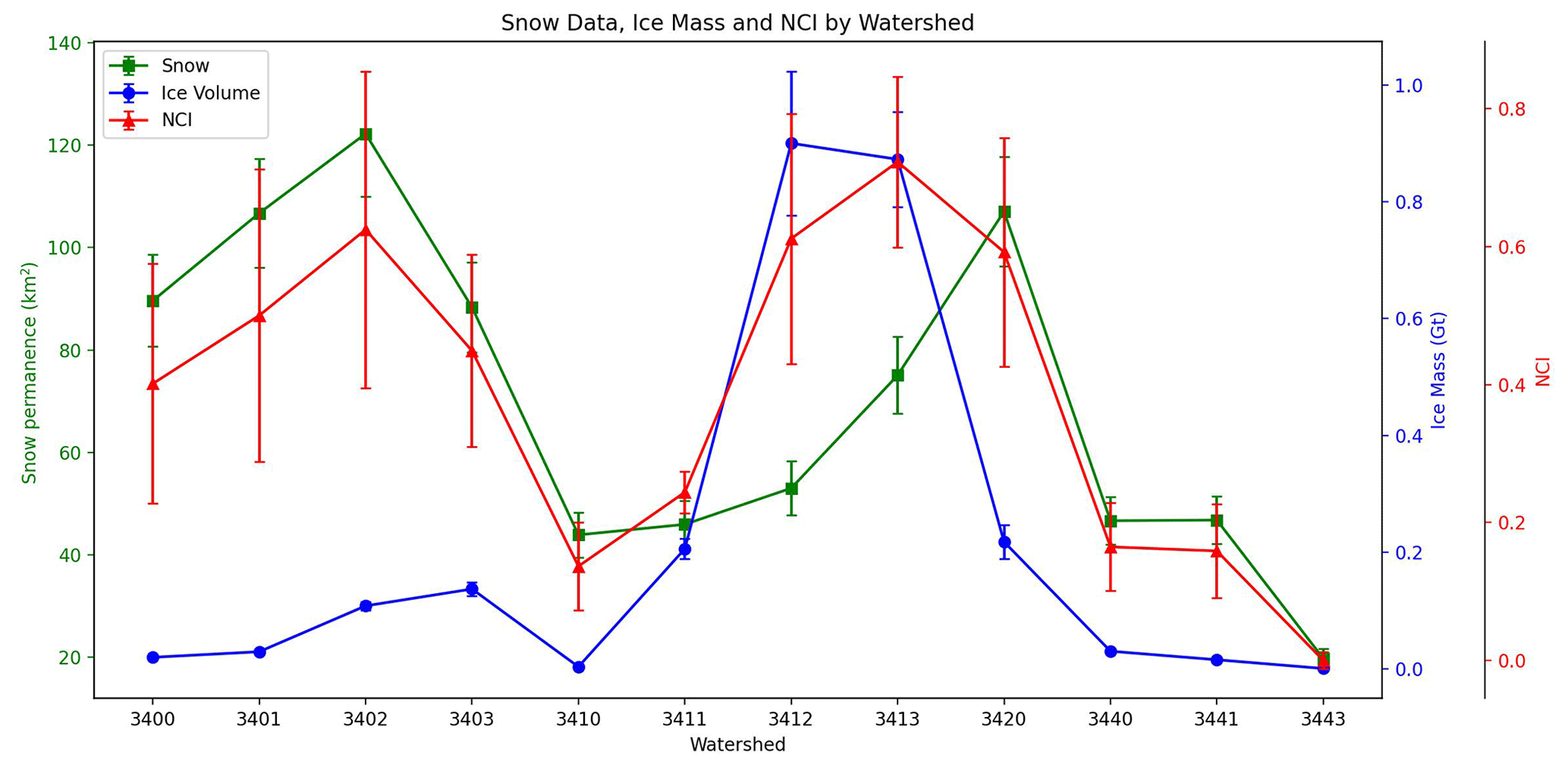
Figure 20 Summary graph of the normalized indexes for snow, cryospheric landforms and the cryosphere for each sub-watershed of the Copiapó River watershed.

5.3 Impact on watershed management

We have analyzed 12 cryospheric sub-watersheds in the Copiapó watershed and showed that there are some that should be prioritized in watershed management strategy. The methodological framework developed and presented in this study can be extended to assess the comprehensive hydrological potential of arid watersheds in high-elevation Andean regions of Chile and other globally distributed arid zones with a focus on cryospheric contributions. In addition, this novel sub-watershed indexing method is fundamental to identify those watersheds with an important snow, glacial and periglacial component that are suitable for inclusion in the watershed protection frameworks that are implemented in the water management strategies of each watershed in Chile. Given the persistent progression of climate change, it is imperative to integrate water reserves sourced from cryospheric watersheds into comprehensive policy-making frameworks governing hydrological regulation.

Implementing and integrating such cryosphere inventories will also allow other regions to preserve their water resources. Currently, the Chilean national cryospheric inventories distinguish between glacier and periglacial landforms. Debris-free and debris-covered glaciers are comprehensively included in the National Glacier Inventory of Chile, whereas within the periglacial environment, only rock glaciers are systematically inventoried. As a result, ice volumes potentially stored in other ice-rich periglacial landforms, such as protalus lobes and gelifluction taluses, are not explicitly accounted for in existing national inventories, despite being addressed in this study. Increasing the variety of cryospheric landforms would facilitate more accurate estimations of the volumes of ice in each sub-watershed, especially in northern Chile where the gelifluction taluses and protalus lobes dominate the cryospheric landforms.

Identifying the strategic position of these sub-watersheds does not imply guaranteeing constant runoff, but rather highlights those sub-watersheds with a higher potential to sustain streamflow under low-snowfall or dry-year conditions. The runoff analysis shows that, during dry years, discharge is strongly reduced but not suppressed, and remains seasonally coupled to melt processes originating in high-elevation cryospheric environments. Sub-watersheds ranked as strategic by the NCI concentrate larger cryospheric landforms and higher snow permanence, which together contribute to buffering runoff variability and maintaining baseflow during periods of limited snowfall. The extraction of precious metals has consumed large quantities of water that was stored in cryospheric landforms (Brenning, 2008). A lack of comprehensive understanding regarding the spatial distribution and volumetric potential of cryospheric water reserves has contributed to the degradation of cryospheric landforms critical for supplying freshwater to downstream populations residing at lower elevations. These sub-watersheds are predominantly cryospheric rather than pluvial in character, indicating that their hydrological regime is mainly influenced by meltwater processes associated with glaciers, ice-rich periglacial landforms, and seasonal snow permanence, particularly during the melt season. When the potential volume of water in each sub-watershed is understood, policy and infrastructure can be adapted to maintain those cryospheric components. Prioritizing the extraction of water from cryospheric landforms and implementing snow capture techniques is essential to ensure the sustainable development and enhanced productivity of the examined region, as well as the arid northern regions of Chile. These sub-watersheds may therefore play an important role in the prevention of water disasters greater than those already known in Chile. The methodological basis developed in this study can be a key-tool for developing a law to protect Chile's cryosphere and its associated water resources when adopted in future water management strategy plans.

6 Conclusions

6.1 Main findings of the paper

We developed a reproducible workflow that maps glacial and periglacial cryospheric landforms and seasonal snow, estimates their ice volumes with a unified physics-based framework, and integrates both into a Normalized Cryospheric Index (NCI) that ranks sub-watersheds with explicit Monte Carlo uncertainty propagation. Applied to the Copiapó watershed, the workflow classified 12 of 27 sub-watersheds as cryospheric; these contain 97 % of the inventoried landforms and overlap 97 % with high-probability permafrost predicted by Gruber (2012), providing independent support for the classification.

The empirical link between September snow extent and October–March discharge at Copiapó River at Pastillo (R²=0.58; r=0.76; N=22) confirms that snow permanence exerts a first-order control on seasonal runoff. The 42 % of unexplained variance is consistent with longer-residence cryospheric storage (rock glaciers, debris-covered ice, ice-rich permafrost) sustaining baseflow during low-snow years, which is precisely the contribution the NCI is designed to capture.

Ice mass is strongly concentrated: the Del Potro (03412; 0.90 Gt) and Montosa (03413; 0.87 Gt) sub-watersheds alone dominate the basin’s cryospheric storage, with Manflas (03420; 0.22 Gt) third. Debris-free glaciers are the principal contributor in these top reservoirs, whereas ice-rich permafrost landforms, particularly gelifluction taluses and rock glaciers, account for a substantial and, at the basin scale, cumulatively important fraction, especially in intermediate and smaller sub-watersheds. Debris-free glaciers are the principal contributor in these top reservoirs, whereas ice-rich permafrost landforms – particularly gelifluction taluses and rock glaciers – account for a substantial and, at the basin scale, cumulatively important fraction, especially in intermediate and smaller sub-watersheds.

The NCI, integrated over the observed 2001–2022 distribution of the ice–snow weighting factor (mean w=0.43), ranks Montosa first (0.72 ± 0.12) and, under dry-year conditions (w=0.62), consistently places Montosa, Del Potro and Manflas as the primary priority sub-watersheds, which together concentrate ∼ 78 % of the ice mass inventoried across the 12 cryospheric sub-watersheds (Table 6). These three are the basins most likely to sustain runoff during droughts and should be prioritized in the national water-resources strategy. Estero Come Caballos (03402; NCI = 0.62 ± 0.23) and Figueroa (03401; NCI = 0.50 ± 0.21) emerge as snow-driven basins that lead the ranking in wet years (w=0.27): in high-snowfall years their hydrological productivity rises, so management there should focus on capturing increased runoff rather than on protecting long-term ice. Adding these two raises the prioritized share of inventoried ice mass to ∼ 84 %. This dual behaviour – southern, ice-rich basins safeguarding dry-year baseflow versus northern, snow-rich basins driving wet-year runoff – is the central management insight of the index.

6.2 Relevant topics detected

Three findings have implications beyond the Copiapó basin. First, gelifluction taluses and protalus lobes – which dominate the arid Atacama cryosphere by extent and store non-negligible ice – are currently excluded from Chile's national periglacial inventory, which systematizes only rock glaciers. Their omission means national ice-storage assessments likely underestimate the periglacial reserve in northern Chile. Second, our ERT surveys returned ice-rich cores ∼ 15 m thick in a gelifluction talus and 20–35 m in an active rock glacier, an order of magnitude greater than thicknesses assumed for analogous landforms in parts of the literature, reinforcing that periglacial ice is being undercounted and warranting targeted geophysical campaigns. Third, the very low DInSAR surface velocities (mm yr⁻¹), one to two orders of magnitude slower than rock glaciers further south in the Dry Andes, are physically consistent with the colder, drier permafrost imposed by proximity to the South American Arid Diagonal and with the predominantly cryogenic (rather than glacigenic) origin of these landforms; this constrains how kinematic models should be transferred across the Andes.

6.3 Limitations and outlook

The NCI is calibrated for the Copiapó watershed and requires complete resource and reserve data to be transferred elsewhere. The main quantified uncertainty in the snow term is the assumed ∼ 10 % accuracy of the MODIS fractional-snow-cover product under ideal conditions; deriving a spatially explicit FSC uncertainty for high-mountain terrain is the priority next step to refine the index. Likewise, the weighting factor w was derived from the 2001–2022 record; under the ongoing megadrought the ice contribution to runoff is expected to increase, so dry-year scenarios should gain weight in future applications of the index. Given projections of reduced glacier meltwater under future Southern Andes megadroughts (Ayala et al., 2025), identifying and protecting high-NCI cryospheric sub-watersheds is increasingly urgent. The framework provides technical, objective input for the DGA, water-monitoring boards and groundwater communities, and offers a methodological basis for integrating glacial and periglacial reserves into watershed-protection policy – and potentially into a legal instrument to protect Chile's cryosphere and its associated water resources.