Impact of blowing snow on the surface radiation balance near the western margin of the Greenland Ice Sheet

Blowing snow sublimation is a key boundary-layer process on the Greenland Ice Sheet that removes and redistributes snow and thereby influences the surface energy balance. However, the direct radiative impacts of blowing snow are often not included in (regional) climate models. This study investigates the influence of blowing snow on the surface radiation balance at observational site S10 near the western margin of the Greenland Ice Sheet using the regional climate model RACMO2.4p1. The radiative properties of the blowing snow layer are described as a low-level ice cloud using the blowing snow mixing ratio, effective radius, and blowing snow cloud fraction, which are taken from the blowing snow routine. Model experiments, both including and excluding blowing snow in the forcing of the stand-alone radiation scheme, are compared to quantify the impact of blowing snow on the surface radiation balance and evaluated against observational data. Our results indicate that blowing snow enhances longwave emissivity and reduces shortwave transmissivity of the near-surface atmosphere, leading to a mean increase of 5.8 W m⁻² in downwelling longwave radiation and a mean decrease of 1.2 W m⁻² in downwelling shortwave radiation at the surface during blowing snow events. Including blowing snow in the radiation scheme improves the simulated surface radiation balance in RACMO2.4p1. The blowing snow routine underestimates peak horizontal transport fluxes by 69 % to 79 % during the short observational period in summer. We recommend coupling blowing snow and radiation schemes in climate models to account for the influence of blowing snow on the local climate and the surface mass balance of the Greenland Ice Sheet.

1 Introduction

The Greenland Ice Sheet (GrIS) has been losing mass in recent decades and has become a major contributor to global mean sea level rise (Horwath et al., 2022; The IMBIE Team et al., 2020; Van den Broeke et al., 2016). Accurately representing the surface mass balance (SMB) in climate models is required to improve projections of the contribution of the GrIS to sea level rise under global warming scenarios (Agosta et al., 2019). While the spatiotemporal variability of the SMB of the GrIS is mainly determined by precipitation and runoff, blowing snow sublimation and erosion are the only processes that remove mass from the ice sheet interior (Lenaerts et al., 2012). This mass removal occurs when strong winds pick up snow from the surface and redistribute it across the GrIS. When this so-called drifting snow is lifted 1.8 m above the surface and is suspended in the atmospheric boundary layer, it is referred to as blowing snow (Serreze and Barry, 2014). Suspended snow is prone to sublimation when the atmospheric boundary layer is undersaturated, which is enhanced by the turbulent flow of air around the particles (Schmidt, 1972). In this study, we use the term “blowing snow” to refer to the combination of both drifting and blowing snow.

Besides its effects on SMB, blowing snow sublimation also influences the local climate by impacting the surface energy balance (SEB). The process of sublimation modifies the temperature and humidity profiles of the lower atmosphere through energy uptake and moisture release (Déry et al., 1998), which in turn affects the surface turbulent heat fluxes (Pomeroy and Essery, 1999; Lenaerts et al., 2010). Yamanouchi and Kawaguchi (1985) have shown that blowing snow also directly influences the surface radiation balance (SRB) at Mizuho Station (Antarctica) through a decrease in the net longwave cooling and downwelling global solar radiation flux at the surface. Moreover, Lesins et al. (2009) observed that downwelling longwave fluxes at the surface increase up to 36 W m⁻² during blowing snow events over rough topography, and Yang et al. (2014) found that upwelling longwave radiation increases at the top of the atmosphere over the East Antarctic Ice Sheet during blowing snow events in winter months.

The impact of blowing snow on the SRB and climatology can be studied on a continental scale using regional climate models (RCMs). Hofer et al. (2021) found that accounting for the radiative effects of blowing snow in the Modèle Atmosphérique Régional (MAR) increases the SRB of the Antarctic Ice sheet. A case study over the Antarctic Peninsula using the snow/ice enhanced Weather Research and Forecasting (WRF-ice) model found that the surface radiation fluxes are the dominant component of the SEB influenced by blowing snow (Luo et al., 2021). An intermediate-complexity parametrisation of blowing snow in the ICOLMDZ atmospheric general circulation model suggests that the increase in SRB due to blowing snow is partly offset by a decrease in the turbulent sensible heat flux (Vignon et al., 2026).

In this study, we use the Regional Atmospheric Climate Model (RACMO2.4p1) of which the blowing snow and cloud schemes have recently been revised (van Dalum et al., 2024; van Dalum et al., 2025). The updated blowing snow routine affects the SMB through blowing snow sublimation and erosion, and influences the SEB through moisture release and energy uptake during sublimation (Gadde and Van De Berg, 2024). However, the direct radiative effects of blowing snow are currently not included in the model. While the revised blowing snow scheme has been evaluated against in situ measurements and satellite observations over Antarctica (Gadde and Van De Berg, 2024), such an evaluation has not yet been performed for Greenland. In addition, the revised cloud scheme of RACMO2.4p1, ecRad-1.4.1 (Hogan and Bozzo, 2018), distinguishes between liquid and ice water content, enabling investigation of the radiative effects of blowing snow by representing it as a low-level ice cloud. The frequent occurrence of blowing snow and availability of both measurements of horizontal blowing snow transport and surface radiation fluxes make observational site S10, which is located in the lower accumulation zone of the GrIS and is part of the Kangerlussuaq (K) transect (inset of Fig. 1; Lenaerts et al., 2014), well-suited for evaluating both the blowing snow routine and the simulated radiative effects of blowing snow over the GrIS.

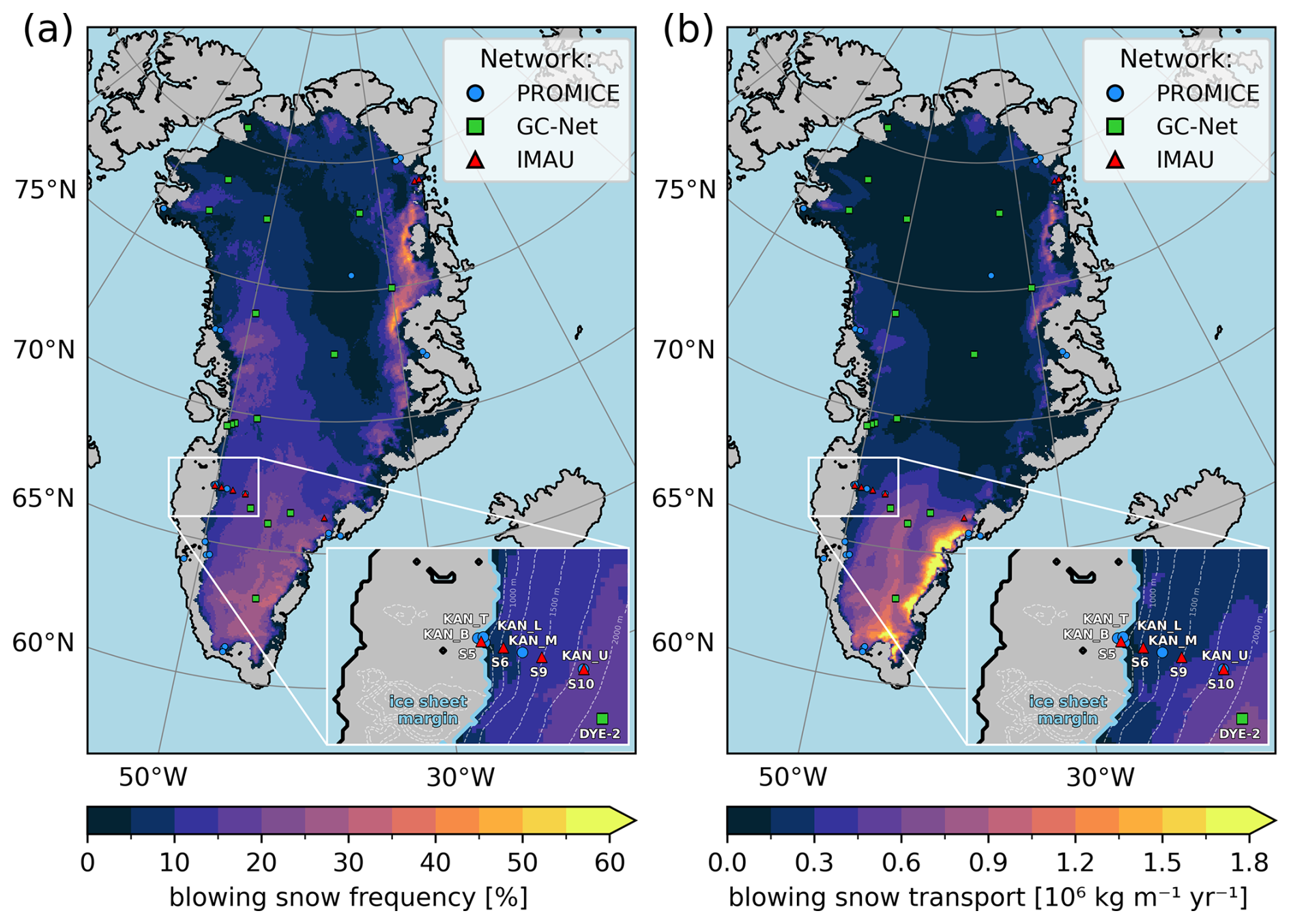
Figure 1 Blowing snow variables simulated by RACMO2.4p1 for the year 2012 across the glaciated regions of Greenland and surroundings: (a) percentage of days with blowing snow (daily mean $Q_{\mathrm{T}}>{\mathrm{10}}^{-\mathrm{3}}$ $\mathrm{kg}{\mathrm{m}}^{-\mathrm{1}}{\mathrm{s}}^{-\mathrm{1}}$), (b) total vertically integrated horizontal blowing snow transport Q_T [$\mathrm{kg}{\mathrm{m}}^{-\mathrm{1}}{\mathrm{yr}}^{-\mathrm{1}}$]. Maps show the locations of the automatic weather stations of the Programme for Monitoring of the Greenland Ice Sheet (PROMICE; blue circles), the Greenland Climate Network (GC-Net; green squares), and the Institute for Marine and Atmospheric Research Utrecht (IMAU; red triangles), and an inset of the Kangerlussuaq (K) transect including the location of S10 and KAN_U, the ice sheet margin (light blue line), and topography (white dashed lines).

This study aims to establish one-way offline coupling between the blowing snow and radiation routines of RACMO2.4p1. The impact of blowing snow on the surface radiation balance is investigated at S10 by comparing experiments including and excluding the radiative effects of blowing snow. Observations of horizontal blowing snow transport and surface radiation fluxes are used to evaluate the performance of RACMO2.4p1 and the experiments with and without the one-way offline coupling between the blowing snow and radiation scheme. The models, their forcing and the experimental data are introduced in Sect. 2. Section 3 highlights the impact and evaluation of forcing the radiation scheme with blowing snow during a case study and for a longer period between 2010 and 2016. The interpretation, implications, and limitations of this work are discussed in Sect. 4, and conclusions and final remarks are made in Sect. 5.

2 Methods and data

2.1 Description of the observations

The observations were obtained in the lower accumulation zone of the GrIS and consist of data from a comprehensive blowing snow experiment run by the IMAU between 6 September 2012 and 7 October 2012 to measure atmospheric profiles and blowing snow transport fluxes (Lenaerts et al., 2014), and from two simultaneously operated automatic weather stations (AWSs) at the same location, i.e. S10 and KAN_U, operated by the IMAU (Smeets et al., 2018) and the Programme for Monitoring of the Greenland Ice Sheet (PROMICE; Fausto et al., 2021). The instruments installed at S10 and KAN_U that are used in this study are listed in Table A1. The stations are located in very close proximity to each other at 67.00° N and 47.02° W, at an elevation of 1850 m, approximately 140 km from the western margin of the GrIS, in its lower accumulation zone (inset of Fig. 1a, b). This site is chosen because of the relatively frequent occurrence of blowing snow and the availability of blowing snow and surface radiation measurements.

Blowing snow occurs across the entire GrIS (Fig. 1a), with the highest frequencies (percentage of days with a daily mean blowing snow transport $Q_{\mathrm{T}}>{\mathrm{10}}^{-\mathrm{3}}$ $\mathrm{kg}{\mathrm{m}}^{-\mathrm{1}}{\mathrm{s}}^{-\mathrm{1}}$) near the ice sheet margins in the northeast (up to 60 % of days), south (up to 40 % of days), and west (up to 30 % of days). The total horizontal blowing snow transport ranges from 0.02×10⁶ $\mathrm{kg}{\mathrm{m}}^{-\mathrm{1}}{\mathrm{yr}}^{-\mathrm{1}}$ on the ice sheet plateau, which is characterized by relatively calm conditions, to more than 2.5×10⁶ $\mathrm{kg}{\mathrm{m}}^{-\mathrm{1}}{\mathrm{yr}}^{-\mathrm{1}}$ near southeastern margins (Fig. 1b), where wind speeds are higher and the surface snow density is relatively low (Lenaerts et al., 2012). Blowing snow occurs on 16 % of days at S10 and KAN_U with a total horizontal snow transport of 0.4×10⁶ $\mathrm{kg}{\mathrm{m}}^{-\mathrm{1}}{\mathrm{yr}}^{-\mathrm{1}}$, making this observational site representative of the blowing snow climate of the entire GrIS in terms of total transport.

2.1.1 Blowing snow experiment

We rely on blowing snow mass flux and friction velocity measurements obtained by Lenaerts et al. (2014) from 6 September 2012 to 7 October 2012 to evaluate the blowing snow routine at S10. A snow particle counter (SPC; Sato et al., 1993) was kept at approximately 1.00±0.15 m above the surface using a vertically adjustable frame connected to an SR50 snow height sensor (Table A1; Lenaerts et al., 2014). To save energy, the SPC was turned off at wind speeds below 5 m s⁻¹, when blowing snow is not expected to occur (Li and Pomeroy, 1997). The set-up also included an 8 m high profile tower equipped with a CSAT3 sonic anemometer (Table A1) at approximately 5 m height, which was used to derive the observed friction velocity.

The SPC is self-steering using a wind vane and measures horizontal particle number fluxes for 64 radius classes with a super-luminescent diode sensor, ranging from 18 to 245 µm (Sugiura et al., 2009). As blowing snow particles approach perfect ice spheres more closely than other forms of snow (Pomeroy and Male, 1988), we assume that the blowing snow particles are perfectly rounded. Therefore, the integrated horizontal mass flux q [$\mathrm{kg}{\mathrm{m}}^{-\mathrm{2}}{\mathrm{s}}^{-\mathrm{1}}$] is given by:

$$\begin{array}{}\text{(1)}& q=\sum _{c_{\mathrm{r}}=\mathrm{1}}^{\mathrm{64}}{q}_{\mathrm{r}}=\sum _{c_{\mathrm{r}}=\mathrm{1}}^{\mathrm{64}}{n}_{\mathrm{r}}{\displaystyle \frac{\mathrm{4}}{\mathrm{3}}}\mathit{\pi }{r}^{\mathrm{3}}{\mathit{\rho }}_{\mathrm{ice}},\end{array}$$

where q_r is the mass flux per radius class [$\mathrm{kg}{\mathrm{m}}^{-\mathrm{2}}{\mathrm{s}}^{-\mathrm{1}}$], c_r is the index of the 64 particle radius classes with median radius r [m], n_r is the measured number flux [${\mathrm{m}}^{-\mathrm{2}}{\mathrm{s}}^{-\mathrm{1}}$], and ρ_ice=917 kg m⁻³ is the density of ice.

The mass flux from the SPC includes the effect of snowfall as the instrument counts particles from both blowing snow transport and snowfall (Sugiura et al., 2009). Because RACMO2.4p1 modelled concurrent snowfall during all major blowing snow events within the measurement period, the method of Naaim-Bouvet et al. (2014) is used to identify and exclude the events in which the measured mass fluxes were severely impacted by snowfall. For blowing snow events without concurrent snowfall, it is known from theory that: (i) blowing snow transport fluxes exhibit a power law with windspeed (Radok, 1977), (ii) observed particle sizes increase with windspeed (Budd et al., 1966), and (iii) snow particle size follows a gamma distribution (Budd et al., 1966; Schmidt, 1981).

The SPC detected 15 blowing snow events in various weather conditions during its operational period (Lenaerts et al., 2014), of which we label the largest five events from A–E during our analysis. Events C and D are excluded from analysis (15 % of datapoints) based on visual inspection of the snowfall detection method of Naaim-Bouvet et al. (2014). The measured snow particle size distributions during the five largest blowing snow events are approximately gamma distributed, as expected from theory (Budd et al., 1966; Schmidt, 1981), except for an anomalous peak in the largest particle radius class (245 µm, not shown). This particle radius class therefore makes a major contribution to the total blowing snow mass transport flux (up to 76 %), whereas contributions from other large particle radius classes were generally below 1 % during blowing snow events without concurrent snowfall. As we could not identify an alternative physical explanation for this observed peak, we surmise that these large particles are precipitating snow and exclude this largest particle radius class from the analysis, following Sugiura et al. (1998).

2.1.2 Automatic weather station observations

We use measurements of the four broadband radiation components from S10 and KAN_U to evaluate modelled radiative fluxes between 18 August 2010 and 22 January 2016, the period of available SRB data from the AWS operated by the IMAU. The downwelling shortwave radiation (SW_↓) measurements from S10 and KAN_U have been corrected for tilt (Smeets et al., 2018; Fausto et al., 2021), and the longwave radiation measurements of S10 have been corrected for the window heating effect due to the absorption of shortwave radiation. The temperature and relative humidity observations of S10, which have been corrected for radiation heating effects (Smeets et al., 2018), are used to evaluate RACMO2.4p1. Both datasets are averaged to an hourly resolution and linearly interpolated to the model output timestamps.

2.2 Description of the models

2.2.1 Regional climate model RACMO2.4p1

We use stand-alone versions of the blowing snow and radiation subroutines from the Regional Atmospheric Climate Model RACMO2.4p1 (hereafter R24). The polar version (“p”) of this hydrostatic model is developed and maintained at the IMAU (van Dalum et al., 2024) and combines the atmospheric dynamics package of the High Resolution Limited Area Model (HIRLAM) version 5.0.3 (Undén et al., 2002) and the physical processes representation of the Integrated Forecast System (IFS) cycle 47r1 of the European Centre for Medium-Range Weather Forecasts (ECMWF, 2020). ERA5 data (Hersbach et al., 2020) are used every three hours to force the model at the lateral boundaries and to nudge the model at the upper boundary (van de Berg and Medley, 2016). R24 was run on the Greenland domain on a 5.5×5.5 km² horizontal resolution with 40 atmospheric levels and a variable model time step of one to five minutes depending on a numerical stability criterion (van Dalum et al., 2024).

2.2.2 Blowing snow model PIEKTUK-D

The blowing snow scheme of R24 is based on the double-moment bulk version of the PIEKTUK-model (hereafter PIEKTUK-D; Déry and Yau, 2001). The model calculates horizontal blowing snow transport fluxes and sublimation from horizontal wind speed, temperature, and humidity profiles (Gadde and Van De Berg, 2024). Blowing snow is simulated when the friction velocity u_* [m s⁻¹] exceeds the threshold friction velocity u_*t [m s⁻¹], which depends on characteristics of the upper snow layer such as density, grain size, dendricity, and sphericity (Gallée et al., 2001). In R24, dendricity and sphericity are not explicitly modelled and are instead prescribed as constant values of 0.5 (Gadde and Van De Berg, 2024). The snow mixing ratio in the saltation layer q_salt [kg kg⁻¹] is calculated using a parametrisation by Pomeroy (1989):

$$\begin{array}{}\text{(2)}& q_{\mathrm{salt}}={\displaystyle \frac{e_{\mathrm{salt}}}{g{h}_{\mathrm{salt}}}}(u_{*}^{\mathrm{2}}-u_{*\mathrm{t}}^{\mathrm{2}}),\end{array}$$

in which $e_{\mathrm{salt}}=\mathrm{1}/\left(\mathrm{3.25}{u}_{*}\right)$ is the dimensionless saltation efficiency which is derived emperically (Pomeroy, 1989), g=9.81 m s⁻² is the gravitational acceleration, and $h_{\mathrm{salt}}=\mathrm{0.08436}{u}_{*}^{\mathrm{1.27}}$ is the height of the saltation layer [m].

The distribution of blowing snow particles in the saltation layer is described by a two-parameter gamma function (Schmidt, 1981):

$$\begin{array}{}\text{(3)}& F\left(r\right)={\displaystyle \frac{N{r}^{(\mathit{\alpha }-\mathrm{1})}{e}^{(-r/\mathit{\beta })}}{{\mathit{\beta }}^{\mathit{\alpha }}\mathrm{\Gamma }\left(\mathit{\alpha }\right)}},\end{array}$$

in which N is the number concentration of snow particles [m⁻³], α=4 and $\mathit{\beta }=\mathrm{100}/\mathit{\alpha }$ [µm] are the shape and scale parameters of the gamma distribution, and $\mathrm{\Gamma }\left(\mathit{\alpha }\right)=(\mathit{\alpha }-\mathrm{1})\mathrm{!}$ is the gamma function. A relation between the bulk (i.e. integrated over the particle size distribution) blowing snow mixing ratio q_b [kg kg⁻¹], snow number concentration N, and mean particle radius r_m [m] is found by assuming that blowing snow particles are perfectly spherical (Déry and Yau, 2001):

$$\begin{array}{}\text{(4)}& r_{\mathrm{m}}=\mathit{\alpha }[{\displaystyle \frac{\mathrm{3}\mathit{\rho }{q}_{\mathrm{b}}\mathrm{\Gamma }\left(\mathit{\alpha }\right)}{\mathrm{4}\mathit{\pi }{\mathit{\rho }}_{\mathrm{ice}}\mathrm{\Gamma }(\mathit{\alpha }+\mathrm{3})N}}{]}^{\mathrm{1}/\mathrm{3}},\end{array}$$

where ρ is the density of air [kg m⁻³]. The distribution of snow particles can be calculated from the snow mixing ratio q_b and number concentration N due to the assumption that α=4 is constant in PIEKTUK-D.

The evolution of q_b and N is governed by eddy diffusivity, settling velocity, and sublimation (Déry and Yau, 2001):

$$\begin{array}{}\text{(5)}& {\displaystyle \frac{\partial q_{\mathrm{b}}}{\partial t}}={\displaystyle \frac{\partial }{\partial z}}(K_{\mathrm{b}}{\displaystyle \frac{\partial q_{\mathrm{b}}}{\partial z}}+v_{\mathrm{b}}{q}_{\mathrm{b}})+S_{\mathrm{b}}\text{(6)}& {\displaystyle \frac{\partial N}{\partial t}}={\displaystyle \frac{\partial }{\partial z}}(K_N{\displaystyle \frac{\partial N}{\partial z}}+v_N{q}_N)+S_N,\end{array}$$

in which z is height above the surface [m] and $K_{\mathrm{b}},K_N=K_{\mathrm{m}}=u_{*}l$ are the eddy diffusivities for q_b and N respectively [m² s⁻¹]. Mixing length $l=(\mathrm{1}/(\mathit{\kappa }\cdot (z+z_{\mathrm{0}\mathrm{m}}))+\mathrm{1}/l_{\max }{)}^{-\mathrm{1}}$ [m] is given by κ(z+z_0m) close to the surface and converges to a maximum of l_max=20 m at increasing heights. v_b and v_N are the bulk settling velocities weighted by the third and first moment respectively [m s⁻¹], and S_b and S_N are the rate of change in the snow mixing ratio [$\mathrm{kg}{\mathrm{kg}}^{-\mathrm{1}}{\mathrm{s}}^{-\mathrm{1}}$] and number concentration [${\mathrm{m}}^{-\mathrm{3}}{\mathrm{s}}^{-\mathrm{1}}$] due to sublimation.

The sublimation mass change is given by the formulation of Thorpe and Mason (1966):

$$\begin{array}{}\text{(7)}& \begin{array}{rl}{\displaystyle \frac{\mathrm{d}m}{\mathrm{d}t}}=& (\mathrm{2}\mathit{\pi }r\mathit{\sigma }-{\displaystyle \frac{Q_{\mathrm{r}}}{K{N}_{\mathrm{Nu}}{T}_{\mathrm{a}}}}[{\displaystyle \frac{L_{\mathrm{s}}}{R_{\mathrm{v}}{T}_{\mathrm{a}}}}-\mathrm{1}\left]\right)/\\ & \left({\displaystyle \frac{L_{\mathrm{s}}}{K{N}_{\mathrm{Nu}}{T}_{\mathrm{a}}}}\right[{\displaystyle \frac{L_{\mathrm{s}}}{R_{\mathrm{v}}{T}_{\mathrm{a}}}}-\mathrm{1}]+{\displaystyle \frac{R_{\mathrm{v}}{T}_{\mathrm{a}}}{N_{\mathrm{Sh}}D{e}_{\mathrm{i}}}}),\end{array}\end{array}$$

in which σ is the water vapour deficit over ice, T_a is the air temperature [K], K is the thermal conductivity of air [$\mathrm{W}{\mathrm{m}}^{-\mathrm{1}}{\mathrm{K}}^{-\mathrm{1}}$], L_s is the latent heat of sublimation [$\mathrm{J}{\mathrm{kg}}^{-\mathrm{1}}{\mathrm{K}}^{-\mathrm{1}}$], R_v is the gas constant for water vapour [$\mathrm{J}{\mathrm{kg}}^{-\mathrm{1}}{\mathrm{K}}^{-\mathrm{1}}$], D is the molecular diffusivity of water vapour through air [m² s⁻¹], Q_r is the net radiation transferred to the ice particles [W], e_i is the vapour saturation pressure over ice [Pa], and N_Nu and N_Sh are the Nusselt and Sherwood numbers.

Steady-state profiles of blowing snow transport and sublimation are computed by convergence of Eqs. (5), (6), and (7) with the mixing ratio and particle concentration in the saltation layer as boundary conditions. Finally, the sublimation rate (−S_b) and latent heat from blowing snow sublimation ($L_{\mathrm{s}}{S}_{\mathrm{b}}/c_p$) are added in the prognostic equations of R24 of atmospheric water vapour and temperature.

2.2.3 Radiation scheme ecRad-1.4.1

EcRad-1.4.1 is the stand-alone version of the IFS radiation scheme (Hogan and Bozzo, 2018), which is incorporated in R24 to calculate radiation fluxes every hour (van Dalum et al., 2024). The scheme uses the Rapid Radiative Transfer Model for Global Climate Models (RRTM-G; Mlawer et al., 1997) to estimate gas optical properties. The IFS cycle 47r1 includes updated greenhouse gas and aerosol concentrations that vary each month but not between years. The 3-D aerosol data are derived from the Copernicus Atmospheric Monitoring Service (CAMS) reanalysis (Bozzo et al., 2020) and trace gases from the Global Environmental Monitoring System (GEMS) and the Monitoring Atmospheric Composition and Climate (MACC) reanalysis (Inness et al., 2013). The optical properties of liquid clouds are calculated using the Suite Of Community RAdiative Transfer codes based on Edwards and Slingo (SOCRATES; Edwards and Slingo, 1996), and the optical properties of ice clouds by Baran et al. (2016). The shortwave and longwave radiation fluxes are computed with the RRTM scheme and are embedded within the Monte Carlo Independent Column Approximation (McICA) framework using an exponential-exponential cloud overlap scheme to calculate the cloud-radiation interactions.

2.3 Coupling the blowing snow and radiation models

We establish one-way offline coupling of PIEKTUK-D with the radiation scheme described above by representing the blowing snow layer as a low-level ice cloud in ecRad-1.4.1. The radiation scheme computes the radiative properties of ice clouds using: (i) ice mixing ratio, (ii) ice cloud effective radius, and (iii) cloud fraction (ECMWF, 2020). Although the effective radius is not used in the current ice optics model of R24 (Baran et al., 2016), other optics models do require this as an input, so we still provide it here. To this end, these three variables are computed from PIEKTUK-D output and passed on to the radiation scheme.

The total ice cloud mass mixing ratio q_total,ice [kg kg⁻¹] is obtained by adding up the specific cloud ice content q_ice and the specific cloud snow content q_snow from R24, and the bulk blowing snow mixing ratio q_blsn from PIEKTUK-D:

$$\begin{array}{}\text{(8)}& q_{\mathrm{total},\mathrm{ice}}=q_{\mathrm{ice}}+q_{\mathrm{snow}}+q_{\mathrm{blsn}}\end{array}$$

The effective radius of the blowing snow particles $r_{\mathrm{e}}^{\mathrm{blsn}}$ [m] is calculated for each model level by combining the definition used in ecRad-1.4.1 (Hogan and Illingworth, 2000) with the assumption that blowing snow particles are perfectly spherical:

$$\begin{array}{}\text{(9)}& r_{\mathrm{e}}^{\mathrm{blsn}}={\displaystyle \frac{\mathrm{3}}{\mathrm{4}}}{\displaystyle \frac{V}{A}}={\displaystyle \frac{\mathrm{3}}{\mathrm{4}}}{\displaystyle \frac{\frac{\mathrm{4}}{\mathrm{3}}\mathit{\pi }{\int }_{\mathrm{0}}^{\mathrm{\infty }}{r}^{\mathrm{3}}n\left(r\right)\mathrm{d}r}{\mathit{\pi }{\int }_{\mathrm{0}}^{\mathrm{\infty }}{r}^{\mathrm{2}}n\left(r\right)\mathrm{d}r}}={\displaystyle \frac{{\int }_{\mathrm{0}}^{\mathrm{\infty }}{r}^{\mathrm{3}}n\left(r\right)\mathrm{d}r}{{\int }_{\mathrm{0}}^{\mathrm{\infty }}{r}^{\mathrm{2}}n\left(r\right)\mathrm{d}r}},\end{array}$$

in which V is the total layer integrated volume of the blowing snow particles [m³], A is the total layer integrated projected area of the blowing snow particles [m²], and n(r) is the spectral number concentration [${\mathrm{m}}^{-\mathrm{3}}{\mathrm{m}}^{-\mathrm{1}}$]. The spectral number concentration is obtained from the particle concentration N, the mean particle radius r_m, and the assumption that the blowing snow particles are gamma distributed with α=4 (Eq. 3).

We combine the effective radius of ice and snow clouds $r_{\mathrm{e}}^{\mathrm{ice},\mathrm{snow}}$ from R24 with the effective radius of the blowing snow layer $r_{\mathrm{e}}^{\mathrm{blsn}}$ from PIEKTUK-D using a mass-weighted mean:

$$\begin{array}{}\text{(10)}& r_{\mathrm{e}}^{\mathrm{total},\mathrm{ice}}=(q_{\mathrm{ice}}+q_{\mathrm{snow}}+q_{\mathrm{blsn}})/({\displaystyle \frac{q_{\mathrm{ice}}+q_{\mathrm{snow}}}{r_{\mathrm{e}}^{\mathrm{ice},\mathrm{snow}}}}+{\displaystyle \frac{q_{\mathrm{blsn}}}{r_{\mathrm{e}}^{\mathrm{blsn}}}})\end{array}$$

Lastly, the cloud fraction of the blowing snow layer a_blsn is set to one when the blowing snow mixing ratio q_blsn is above 10⁻⁶ kg kg⁻¹, and equal to zero when q_blsn is below 10⁻⁶ kg kg⁻¹. This threshold is chosen arbitrarily and differs from the approach of Vignon et al. (2026), who assume blowing snow cloud fraction linearly increases with blowing snow mixing ratio and is equal to one for $q_{\mathrm{blsn}}={\mathrm{10}}^{-\mathrm{3}}$ kg kg⁻¹.

The total cloud fraction a_total is computed by combining the liquid, ice and mixed-phase cloud fraction a_liquid,ice from R24 and the cloud fraction of the blowing snow layer a_blsn from PIEKTUK-D:

$$\begin{array}{}\text{(11)}& a_{\mathrm{total}}=\mathrm{1}-(\mathrm{1}-a_{\mathrm{liquid},\mathrm{ice}})(\mathrm{1}-a_{\mathrm{blsn}})\end{array}$$

As a result, the total cloud fraction a_total is equal to one during blowing snow events where $q_{\mathrm{blsn}}>{\mathrm{10}}^{-\mathrm{6}}$ kg kg⁻¹, and a_total is equal to a_liquid,ice otherwhise.

2.4 Simulation setup and model forcing

We force the stand-alone versions of PIEKTUK-D and ecRad-1.4.1 with instantaneous R24 output of the grid cell closest to the coordinates of S10 and KAN_U. We use an hourly resolution from 6 September 2012 until 7 October 2012 to evaluate the blowing snow scheme with the SPC measurements and to investigate the radiative effects of blowing snow in a case study. Additionally, we use 3-hourly data from 18 August 2010 until 22 January 2016, the period with continuous SRB observations at S10, to evaluate ecRad-1.4.1 for a longer time.

PIEKTUK-D requires a fine vertical resolution to accurately model the sublimation of blowing snow, as horizontal snow transport peaks near the surface and vertical gradients of snow mixing ratios are typically steepest there (Déry and Yau, 1999). Therefore, we interpolate horizontal wind speed, temperature, and humidity profiles of R24 to a log-linear blowing snow grid of 8 levels between 0.1 m and the lowest atmospheric model level of R24 (∼10 m). This interpolation is also performed internally in R24 and uses the stability functions of Holtslag and De Bruin (1988) for stable conditions and Dyer (1974) for unstable conditions. The Monin-Obukhov length L [m] is recomputed from the turbulent surface fluxes, as it is not available in the R24 output. PIEKTUK-D uses several substeps to converge the blowing snow mixing ratio, number concentration, and sublimation profiles (Eqs. 5, 6 and 7) to a steady state (Gadde and Van De Berg, 2024). We use 15 substeps in the offline simulations instead of 5 in R24 due to the higher temporal resolution of the forcing. The offline version of PIEKTUK-D includes two bug fixes compared to R24: (i) the blowing snow grid was not correctly aligned to the RACMO vertical levels, and (ii) Eq. (4) was implemented with α=2 instead of the correct value α=4.

EcRad-1.4.1 is directly forced with skin temperature, solar zenith angle, specific humidity, and cloud composition from R24 output. Within R24, cloud composition is differentiated into liquid, rain, ice, and snow water content, and distinct parametrisations are used to calculate liquid and ice effective radii. While the solar irradience has been updated to a variable number around 1361 W m⁻² in R24, it has been set to 1366 W m⁻² for the R24 Greenland run, which is used throughout this study (van Dalum et al., 2024). Therefore, we keep the downwelling solar radiation at the top of the atmosphere constant at 1366 W m⁻², use the broadband albedo of R24 instead of the spectral albedo, and set the surface emissivity to 0.98, the value used in R24 over ice sheets. Downwelling longwave radiation (LW_↓) is increased by 1 %, following R24 (van Dalum et al., 2024) and the half-level temperature is derived from full levels using pressure-weighted interpolation following ECMWF (2020). The aerosol mass mixing ratios and trace gas volume mixing ratios are interpolated to the R24 full-model levels using linear interpolation. The cloud overlap parameter α_c is calculated with the definition of Hogan and Illingworth (2000):

$$\begin{array}{}\text{(12)}& {\mathit{\alpha }}_{\mathrm{c}}=\exp (-{\displaystyle \frac{\mathrm{\Delta }z}{\mathrm{\Delta }{z}_{\mathrm{0}}}}),\end{array}$$

in which Δz is the model level separation [m] and $\mathrm{\Delta }{z}_{\mathrm{0}}=\mathrm{0.75}+\mathrm{2.149}\cos \mathit{\varphi }$ is the decorrelation distance [m] calculated using the latitude ϕ. When α_c=0, the overlap between clouds is completely random and when α_c=1, the overlap between clouds is maximally correlated (Hogan and Illingworth, 2000).

EcRad-1.4.1 provides the downwelling and upwelling shortwave and longwave radiation fluxes at half levels, which are used to calculate net radiation and heating profiles:

$$\begin{array}{}\text{(13)}& {\displaystyle \frac{\partial T}{\partial t}}=-{\displaystyle \frac{g}{c_p}}{\displaystyle \frac{\partial F}{\partial p}},\end{array}$$

where $\frac{\partial T}{\partial t}$ is the heating rate [K s⁻¹], c_p=1004 $\mathrm{J}{\mathrm{kg}}^{-\mathrm{1}}{\mathrm{K}}^{-\mathrm{1}}$ is the specific heat of dry air at constant pressure, F is the net radiation flux [W m⁻²], and p is the pressure [Pa].

We perform three experiments with varying levels of one-way coupling of PIEKTUK-D and ecRad-1.4.1 to investigate the impact of blowing snow on the SRB (Fig. 2). In the baseline experiment (BL), the radiation model is only forced with R24 output. This is the current state of R24, meaning that the impact of blowing snow on radiation is not included. In the RACMO grid experiment (RG), ecRad-1.4.1 is forced with a combination of the output of R24 and PIEKTUK-D at the 40 full atmospheric levels of R24. This means that the effects of blowing snow are neglected beneath the lowest model layer of R24 (∼ 10 m), where blowing snow mixing ratios are highest. Finally, in the integrated grid experiment (IG), blowing snow is included at the atmospheric model levels of R24, and the lowest level of R24 incorporates the integrated mixing ratio and effective radius of the blowing snow grid levels between the surface and the lowest R24 level. Hence, this experiment accounts for the radiative effects of blowing snow close to the surface without introducing additional model levels.

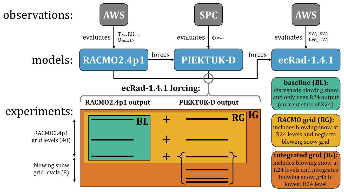
Figure 2 Schematic overview of the methods with the used observations and models, and the three conducted experiments.

3 Results

3.1 Model evaluation

3.1.1 Evaluation of RACMO2.4p1

We first assess the ability of R24 to simulate the relevant input variables of the blowing snow routine at S10. Figure B1 shows the observed and simulated hourly average 2 m temperature, 2 m relative humidity, 10 m horizontal wind speed, and friction velocity during the operational period of the SPC from 6 September 2012 to 7 October 2012. R24 simulates 2 m temperature and 10 m horizontal wind speed with high R² scores of 0.78 and 0.73, and low biases of −1.38 °C and −0.68 m s⁻¹, respectively (Fig. B1a, c). van Dalum et al. (2024) report lower biases of −0.63 °C for 2 m temperature and −0.39 m s⁻¹ for 10 m wind speeds when evaluating R24 against multiple IMAU and PROMICE AWSs for a longer observational period. The observed variability of 2 m relative humidity and friction velocity is captured less well by R24 at S10, with lower R² scores of 0.42 and 0.55, respectively (Fig. B1b, d).

3.1.2 Evaluation of blowing snow model PIEKTUK-D

The stand-alone version of PIEKTUK-D accurately replicates the integrated horizontal blowing snow transport fluxes and sublimation rates of R24, with high R² scores of 0.97 and 0.99, and low biases of 0.35 $\mathrm{g}{\mathrm{m}}^{-\mathrm{2}}{\mathrm{s}}^{-\mathrm{1}}$ and −0.02 mm d⁻¹, respectively (Fig. C1a, b). Figure 3a shows the measured and simulated horizontal blowing snow mass transport fluxes at S10. Most blowing snow events are accompanied by concurrent snowfall rates above 10⁻⁴ $\mathrm{kg}{\mathrm{m}}^{-\mathrm{2}}{\mathrm{h}}^{-\mathrm{1}}$ in R24. During events C and D, observations do neither exhibit a power law between horizontal blowing snow transport and wind speed (Fig. 3b), nor a linear relation between mean particle radius and wind speed (Fig. 3c). The snowfall detection method of Naaim-Bouvet et al. (2014) therefore indicates that the SPC measurements of events C and D are severely impacted by snowfall, whereas the influence of snowfall during events A, B, and E is modest. During these blowing snow events (A, B, and E), the peak simulated horizontal mass transport fluxes are underestimated by 69 % to 79 % compared to observed transport fluxes, consistent with the findings of Gadde and Van De Berg (2024) during austral summer using the same model over Antarctica. Moreover, the blowing snow scheme overestimates horizontal transport fluxes during the onset of events B, D and E, resulting in an R² score of 0.50 and a bias of −0.53 $\mathrm{g}{\mathrm{m}}^{-\mathrm{2}}{\mathrm{s}}^{-\mathrm{1}}$ (Fig. C1c) even though the model captures the timing of the blowing snow events well.

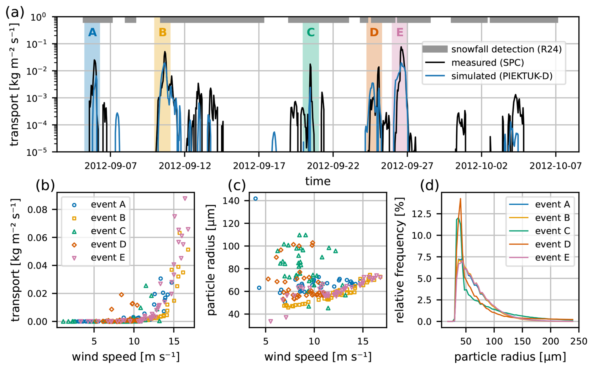
Figure 3 SPC measurements at S10 from 6 September 2012 to 7 October 2012 (the operational period of the SPC) with the five largest blowing snow events highlighted by different colors: (a) comparison of measured (black) and simulated (blue) horizontal blowing snow transport fluxes [$\mathrm{kg}{\mathrm{m}}^{-\mathrm{2}}{\mathrm{s}}^{-\mathrm{1}}$] with simulated snowfall rates above 10⁻⁴ $\mathrm{kg}{\mathrm{m}}^{-\mathrm{2}}{\mathrm{h}}^{-\mathrm{1}}$ indicated by the grey bar at the top, (b) variations of measured horizontal blowing snow transport with measured 1 m wind speed [m s⁻¹], (c) variations of measured mean snow particle radius [µm] with measured 1 m wind speed, and (d) measured blowing snow particle size distributions.

3.1.3 Evaluation of radiation scheme ecRad-1.4.1

The baseline experiment (BL) of the offline ecRad-1.4.1 version, which does not include the radiative effects of blowing snow, correctly replicates the surface radiation fluxes of R24, with high R² scores of 1.00 for shortwave fluxes and 0.99 for longwave fluxes, and biases below 1.5 W m⁻² (Fig. D1). Figure 4 shows the performance of the BL experiment compared to observations at S10 when blowing snow is and is not simulated by PIEKTUK-D, using a threshold of $Q_{\mathrm{T}}={\mathrm{10}}^{-\mathrm{3}}$ $\mathrm{kg}{\mathrm{m}}^{-\mathrm{1}}{\mathrm{s}}^{-\mathrm{1}}$. The BL experiment simulates SW_↓ well, with high R²=0.97 in both cases and low biases of −0.4 W m⁻² without and -3.2 W m⁻² with blowing snow (Fig. 4a, b). On the other hand, the BL experiment underestimates LW_↓ with lower R² scores of 0.45 and 0.38 and larger model biases of −22.9 and −22.6 W m⁻² without and with blowing snow, respectively (Fig. 4c, d), which is a well-known deficiency of R24 (van Dalum et al., 2024).

Figure 4 Density scatter plots of the simulated and observed surface radiation fluxes for the baseline experiment at site S10 without ($Q_{\mathrm{T}}<{\mathrm{10}}^{-\mathrm{3}}$ $\mathrm{kg}{\mathrm{m}}^{-\mathrm{1}}{\mathrm{s}}^{-\mathrm{1}}$) and with blowing snow ($Q_{\mathrm{T}}>{\mathrm{10}}^{-\mathrm{3}}$ $\mathrm{kg}{\mathrm{m}}^{-\mathrm{1}}{\mathrm{s}}^{-\mathrm{1}}$) between 2010 and 2016: (a, b) downwelling surface shortwave radiation flux SW_↓ without and with blowing snow [W m⁻²], (c, d) downwelling surface longwave radiation flux LW_↓ without and with blowing snow [W m⁻²]. Dashed lines represent the 1:1 line, solid lines represent the linear regression line, and the colours represent the normalised point density from low (0.0, dark blue) to high (1.0, red).

3.2 Impact of blowing snow on radiation

3.2.1 Case study: blowing snow during clear-sky conditions

Next, we show the impact of forcing ecRad-1.4.1 with PIEKTUK-D output using a case study from 12 October 2012 to 17 October 2012. This event was selected due to the large vertically integrated horizontal blowing snow transport fluxes, reaching up to 0.4 $\mathrm{kg}{\mathrm{m}}^{-\mathrm{1}}{\mathrm{s}}^{-\mathrm{1}}$, and small background liquid and ice water paths (LWP, IWP) from simulated clouds in R24. The impact of blowing snow on the SRB is more pronounced during clear-sky conditions when SW↓ is large and atmospheric emissivity is near its lower limit, allowing blowing snow to both substantially lower SW↓ and increase LW↓. Figure 5 shows hourly input (panels a–c) and output (panels d–g) of ecRad-1.4.1 during this blowing snow event. The largest background LWP and IWP are observed during short episodes of snowfall in the afternoon of 14 October 2012 and the morning of 15 October 2012 (Fig. 5b). The BL experiment simulates SW_↓ fluxes accurately during the overcast and snowfall conditions, but underestimates SW_↓ during clear-sky conditions on 12 October 2012, 13 October 2012, and 16 October 2012 (Fig. 5d). Moreover, the BL experiment consistently underestimates LW_↓ (Fig. 5f), which is in line with Fig. 4c and d, and findings of van Dalum et al. (2024).

Figure 5 Timeseries of hourly input and output of ecRad-1.4.1 at S10 during a blowing snow event from 12 October 2012 until 17 October 2012 for the baseline (BL, green), RACMO grid (RG, yellow), and integrated grid (IG, orange) experiments: (a) vertically integrated horizontal blowing snow transport flux Q_T [$\mathrm{kg}{\mathrm{m}}^{-\mathrm{1}}{\mathrm{s}}^{-\mathrm{1}}$] simulated by PIEKTUK-D, (b) BL liquid- and ice water path LWP & IWP [kg m⁻²] simulated by RACMO2.4p1, (c) difference in IWP due to blowing snow compared to BL [kg m⁻²], (d, f) downwelling surface shortwave and longwave radiation fluxes SW_↓ and LW_↓ [W m⁻²], (e, g) difference in SW_↓ and LW_↓ due to blowing snow compared to BL [W m⁻²].

Including blowing snow in the forcing of ecRad-1.4.1 decreases SW_↓ and increases LW_↓ at the surface (Fig. 5e, g), with exceptions of SW_↓ on 14 October 2012 at 16:00 UTC and LW_↓ on 13 October 2012 at 20:00 UTC. The increase in IWP due to blowing snow particles during this case study is proportional to the vertically integrated horizontal blowing snow transport Q_T for both the RG and IG experiment, and an order of magnitude smaller than the background LWP and IWP from clouds and snowfall (Fig. 5a, b, c). Therefore, the impact of blowing snow on surface radiation fluxes is best observed during the evening of 12 October 2012 or the morning of 14 October 2012, when background LWP and IWP are smallest.

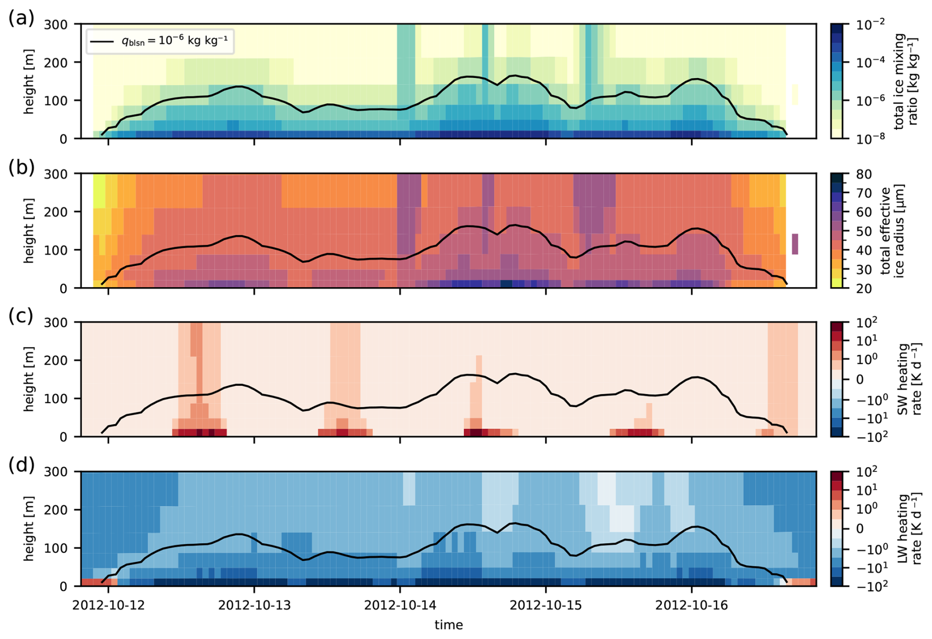
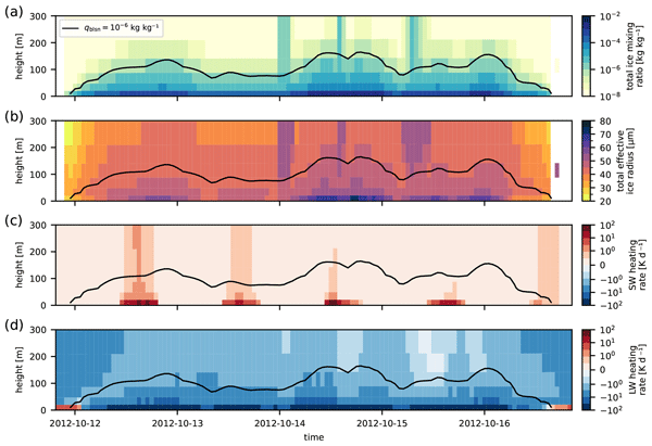
Figure 6 Timeseries of hourly input and output profiles of ecRad-1.4.1 for the integrated grid (IG) experiment during a blowing snow event at S10 from 12 October 2012 until 17 October 2012: (a) total ice mixing ratio (including blowing snow) q_total,ice [kg kg⁻¹], b) total effective radius of ice particles $r_{\mathrm{e}}^{\mathrm{total},\mathrm{ice}}$ [µm], (c, d) net shortwave and longwave heating rates [K d⁻¹]. The black line represents the height at which the blowing snow mixing ratio $q_{\mathrm{blsn}}={\mathrm{10}}^{-\mathrm{6}}$ kg kg⁻¹, indicating the approximate height of the top of the blowing snow layer.

The hourly input and output profiles of the IG experiment during the case study are shown in Fig. 6. The blowing snow layer ($q_{\mathrm{blsn}}>{\mathrm{10}}^{-\mathrm{6}}$ kg kg⁻¹) extends up to ∼ 175 m, and blowing snow mixing ratios and effective radii are largest near the surface, and decrease with height (Fig. 6a, b). The total ice mixing ratio and ice effective radii increase above the blowing snow layer during the three episodes of snowfall. Blowing snow increases the shortwave heating rates of the atmospheric layer near the surface from ∼ 1 K d⁻¹ in BL (not shown) up to 35 K d⁻¹ in IG due to the absorption of shortwave radiation, and decreases the longwave cooling rates from ∼ 1 K d⁻¹ in BL (not shown) up to 150 K d⁻¹ in IG due to increased atmospheric emissivity (Fig. 6c, d).

3.2.2 Total impact between 2010–2016

The RACMO grid (RG) and integrated grid (IG) experiments are compared to observations at S10 during blowing snow events ($Q_{\mathrm{T}}>{\mathrm{10}}^{-\mathrm{3}}$ $\mathrm{kg}{\mathrm{m}}^{-\mathrm{1}}{\mathrm{s}}^{-\mathrm{1}}$) during the AWS operational period from 2012 and 2016 (Fig. 7). Forcing ecRad-1.4.1 with blowing snow in the IG experiment results in an average decrease in SW_↓ of 1.2 W m⁻² and an average increase in LW↓ of 5.8 W m⁻² during blowing snow events compared to the BL experiment. Differences between the RG and BL experiments are smaller (ΔSW${}_{\downarrow }=-\mathrm{0.5}$ W m⁻², ΔLW${}_{\downarrow }=+\mathrm{2.4}$ W m⁻²) because the blowing snow grid levels close to the surface, which contain the largest blowing snow mixing ratios, are neglected in this experiment (Fig. 2). For SW_↓, the RG and IG experiments perform similarly to the BL experiment, with R²=0.97 and slightly higher biases of −3.7 and −4.6 W m⁻², respectively (Fig. 7a, b). The performance in simulating LW_↓ improves for both the RG and IG experiments with larger R² scores, smaller root mean square error (RMSE), and smaller biases (Fig. 7c, d), where the IG performs best with an R²=0.5 and a LW_↓ bias of −16.7 W m⁻². Overall, the SRB improves most in the IG experiment, with a 3.4 W m⁻² reduction in RMSE and a 4.6 W m⁻² reduction in bias during blowing snow events compared to the BL experiment, as the improvement in LW_↓ exceeds the deterioration in SW_↓.

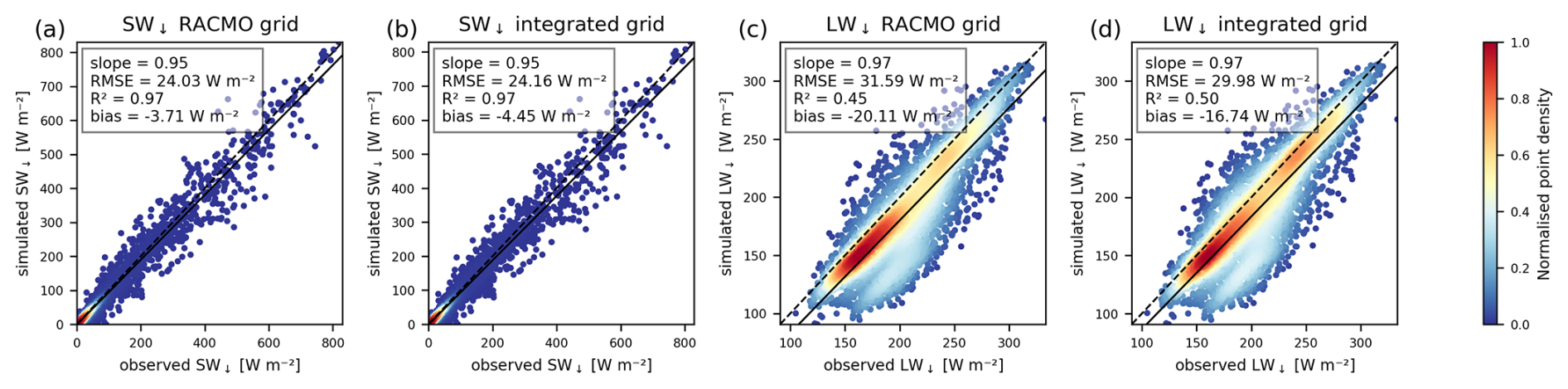
Figure 7 Density scatter plots of the simulated and observed surface radiation fluxes at site S10 during blowing snow events ($Q_{\mathrm{T}}>{\mathrm{10}}^{-\mathrm{3}}$ $\mathrm{kg}{\mathrm{m}}^{-\mathrm{1}}{\mathrm{s}}^{-\mathrm{1}}$) between 2010 and 2016 for the RACMO grid (RG) and integrated grid (IG) experiments: (a, b) downwelling surface shortwave radiation flux SW_↓ of the RG and IG experiments [W m⁻²], (c, d) downwelling surface longwave radiation flux LW_↓ from the RG and IG experiments [W m⁻²]. Dashed lines represent the 1:1 line, solid lines represent the linear regression line, and the colours represent the normalised point density from low (0.0, dark blue) to high (1.0, red).

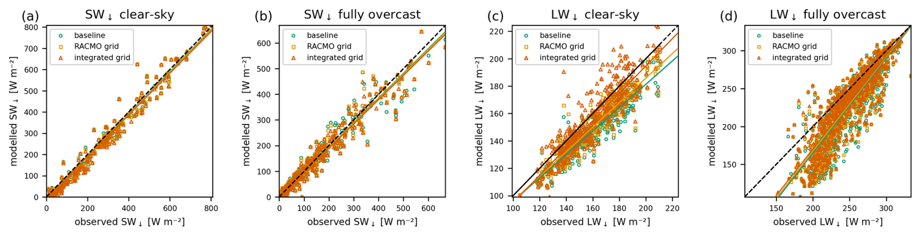
Figure 8 Scatter plots of the simulated and observed surface radiation fluxes at site S10 during blowing snow events between 2010 and 2016 ($Q_{\mathrm{T}}>{\mathrm{10}}^{-\mathrm{3}}$ $\mathrm{kg}{\mathrm{m}}^{-\mathrm{2}}{\mathrm{s}}^{-\mathrm{1}}$) for clear-sky (cloud fraction < 0.2) and fully overcast conditions (cloud fraction > 0.8) following the method of Van Den Broeke et al. (2006) and Kuipers Munneke et al. (2011): (a, b) downwelling surface shortwave radiation flux SW_↓ [W m⁻²], (c, d) downwelling surface longwave radiation flux LW_↓ [W m⁻²]. Dashed lines represent the 1:1 line, solid lines represent the best-fit line, and the colours represent the experiments: baseline (BL, green), RACMO grid (RG, yellow), and integrated grid (IG, red).

The simulated radiation fluxes of the BL, RG, and IG experiments are compared to observations at S10 in Fig. 8 during blowing snow events when R24 correctly simulates little to no clouds or fully overcast conditions. Datapoints are selected when both the simulated cloud fraction of R24 and the observed cloud fraction are below 0.2 for clear-sky conditions and above 0.8 for the fully overcast conditions. The cloud fraction is estimated from observations following the method of Van Den Broeke et al. (2006) and Kuipers Munneke et al. (2011). The method assumes that the clear-sky (cloud fraction = 0) and fully overcast (cloud fraction = 1) conditions are represented by a second-order polynomial fitted to the 5th and 95th percentile levels of LW_↓ plotted against 2 m temperature. Cloud fractions in between these lower and upper bounds are obtained by a linear interpolation between the fitted polynomials. Note that the resulting estimates are subject to uncertainty. Again, forcing ecRad-1.4.1 with PIEKTUK-D output decreases SW_↓ and increases LW_↓ during both experiments, but the impact of coupling is most clearly visible in LW_↓ during clear-sky conditions (Fig. 8c), as discussed above.

4 Discussion

R24 simulates Greenland Ice Sheet (GrIS) near-surface temperature and horizontal wind speed well, and relative humidity and friction velocity with acceptable performance during the observational period of the SPC (6 September 2012 to 7 October 2012) at AWS location S10, which is deemed representative of blowing snow events on the GrIS. The blowing snow model PIEKTUK-D forced by R24 underestimates peak horizontal blowing snow transport fluxes compared to SPC measurements, while the timing of blowing snow events is captured well. We find that blowing snow increases the SRB at S10 by suppressing longwave radiative cooling of the surface, which is only partly offset by a decrease in downwelling shortwave radiation. Within the blowing snow layer, the atmospheric emissivity increases while the shortwave transmissivity decreases, leading to a net cooling of the near-surface atmosphere. Representing blowing snow as a low-level ice cloud in the forcing of ecRad-1.4.1 improves agreement between the simulated and observed downwelling longwave radiation fluxes at S10 but slightly deteriorates the performance of modelled downwelling shortwave radiation fluxes.

The underestimation of simulated peak horizontal blowing snow transport fluxes by PIEKTUK-D during summer is also reported by Gadde and Van De Berg (2024), who evaluate the same model using data from acoustic blowing snow sensors over Antarctica (Amory, 2020). Note that the difference between the horizontal blowing snow transport fluxes of the SPC at S10 in this study and those reported by Lenaerts et al. (2014) could not be explained. While this underestimation can be partially explained by the underestimation of horizontal wind speeds at S10, it could also be related to an underestimated availability of loose surface snow due to inaccuracies in the surface snow compaction model (Gadde and Van De Berg, 2024). For example, overly rapid surface snow compaction in summer could reduce the availability of loose snow and consequently increase the threshold friction velocity (Gallée et al., 2001). Also, R24 does not resolve direct interactions between precipitation and blowing snow, such as precipitating snow acting as an additional source of blowing snow before it reaches the ground (Gadde and Van De Berg, 2024). The modelled blowing snow transport flux is highly sensitive to the surface snow density and particle size distribution within the saltation layer (Lenaerts et al., 2014; Gadde and Van De Berg, 2024). Therefore, future research should focus on improving the spatiotemporal variability of the modelled characteristics of surface snow in R24, such as density, dendricity, and sphericity, and on constraining the particle size distribution across Greenland using in situ measurements. Additional observations, both at other locations and over longer time periods, are required to evaluate PIEKTUK-D's ability to capture the spatial and seasonal dynamics of blowing snow transport and sublimation over the GrIS.

We find that representing a blowing snow layer as a near-surface ice cloud improves the simulated SRB on the GrIS. The simulated impacts of blowing snow on the SRB are consistent with previous observations (Yamanouchi and Kawaguchi, 1985; Lesins et al., 2009; Yang et al., 2014) and modelling studies (Hofer et al., 2021; Le Toumelin et al., 2021; Luo et al., 2021; Vignon et al., 2026). Including the radiative effects of blowing snow reduces biases in downwelling longwave radiation in R24, particularly under clear-sky conditions, as well as in other RCMs (Hofer et al., 2021; Le Toumelin et al., 2021). Part of the residual bias in R24 might be related to deficiencies in cloud representation, such as an underestimated occurence of thin, high-altitude clouds, an underestimation of cloud mixing ratios, and biases in cloud phase partitioning (Feenstra et al., 2026). The underestimation of downwelling shortwave fluxes at S10 during blowing snow events in the baseline experiment could not be explained. Although the absence of direct observations makes it difficult to assess how physically realistic the simulated radiative heating rates in the blowing snow layer are, their order of magnitude appears coherent with the steep gradients in blowing snow mixing ratio in the shallow model layer near the surface. It is therefore realistic that the simulated values are larger than typical cloud heating rates and even exceed the maximum cloud-top cooling rates of −120 K d⁻¹ observed in single-layer low-level liquid clouds using tethered balloon measurements over Svalbard (Lonardi et al., 2024). While ice mixing ratios are higher than normal cloud mixing ratios over the GrIS (Feenstra et al., 2026), the blowing snow layer is much thinner. Therefore, the increase in IWP due to blowing snow is modest, consistent with findings of Hofer et al. (2021). As a result, the impact of blowing snow on downwelling shortwave and longwave radiation fluxes is smaller than the typical influence of clouds (Cawkwell and Bamber, 2002).

The validity of using the ice optics model of R24 to simulate the impact of blowing snow on the SRB remains an assumption, as this parametrisation was specifically developed for cirrus clouds and not blowing snow (Baran et al., 2016). Even though studies suggest that the effective emissivity of the blowing snow layer is similar to that of cirrus clouds, which are composed of ice particles that resemble blowing snow (Yamanouchi and Kawaguchi, 1985), the performance of this ice optics model in simulating the radiative effects of blowing snow should be investigated in more detail. Furthermore, future research should constrain the value or parameterisation of the selected mixing ratio threshold used to determine the cloud fraction of the blowing snow layer (Vignon et al., 2026) and investigate more sophisticated formulations of the effective radius of blowing snow particles, for example, depending on snow properties such as snow age.

The one-way offline coupling between PIEKTUK-D and ecRad-1.4.1 does not incorporate feedbacks between the direct radiative effects of blowing snow, other SEB components, and blowing snow sublimation. For example, radiative cooling of the near-surface atmosphere affects sensible heat fluxes (Vignon et al., 2026) and sublimation rates of blowing snow. Furthermore, blowing snow alters the surface albedo by spectrally modifying incoming radiation, although this influence appears to be limited (Yamanouchi and Kawaguchi, 1985). Lastly, blowing snow not only enhances cloud formation by increasing atmospheric humidity through sublimation, but blowing snow particles can also potentially act as ice-nucleating particles (Hofer et al., 2021). To quantify the impact of blowing snow on the SRB and SMB for the entire GrIS, full coupling should be established between the blowing snow and radiation routines in climate models such as R24. While the increase in SRB is unlikely to considerably increase melt at S10 due to the high elevation and low temperatures, the effect is expected to be larger near the margins of the GrIS and could improve SMB estimates. In coastal Greenland, the direct radiative impacts of blowing snow will likely be less pronounced due to more frequent cloudy conditions. Secondary radiative effects could potentially be amplified due to the interactions between blowing snow and (low-level) clouds discussed above. Moreover, the impacts of blowing snow on the SRB are presumably greater over Antarctica due to a thicker blowing snow layer that can extend hundreds of kilometres horizontally (Hofer et al., 2021).

5 Conclusions

This paper describes a one-way offline coupling between the blowing snow and radiation schemes of the Regional Atmospheric Climate Model RACMO2.4p1 by representing blowing snow as a low-level ice cloud. The radiative properties of this blowing snow cloud are described by the blowing snow mixing ratio, effective radius, and blowing snow cloud fraction, which are computed from the stand-alone blowing snow model PIEKTUK-D, and then given to the radiation model ecRad-1.4.1. The impact of blowing snow on the surface radiation budget is quantified and evaluated at the observational site S10 near the western margin of the Greenland Ice Sheet using three model experiments, including and excluding the direct radiative effects of blowing snow.

We find that blowing snow increases the surface radiation budget at S10 by enhancing downwelling longwave radiation on average with 5.8 and up to 50 W m⁻² during blowing snow events, which is only partly offset by a mean decrease of 1.2 W m⁻² in downwelling shortwave radiation. Including the direct radiative effects of blowing snow improves the agreement with the observed surface radiation balance, particularly for downwelling longwave radiation. While the blowing snow routine captures the timing of the blowing snow events well, peak horizontal transport fluxes are underestimated by 69 % to 79 % during a short observational period in summer, highlighting the importance of further model improvement and evaluation over Greenland. Based on our study, we recommend coupling the blowing snow and radiation schemes in climate models to incorporate the direct radiative effects of blowing snow. This will allow the further investigation of the impact of blowing snow on the local climate and surface mass balance across the Greenland Ice Sheet.

Appendix A: Overview of the instruments used in this study

Table A1 List of instruments installed at S10 and KAN_U and used in this study.

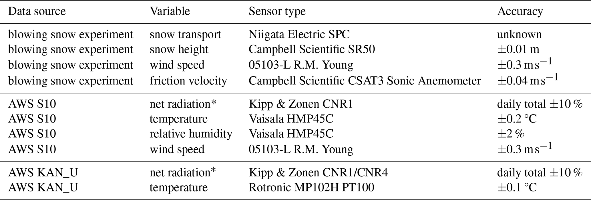
^* The sensor separately measures the upwelling and downwelling shortwave and longwave radiation fluxes.

Appendix B: Evaluation of the Regional Atmospheric Climate Model RACMO2.4p1

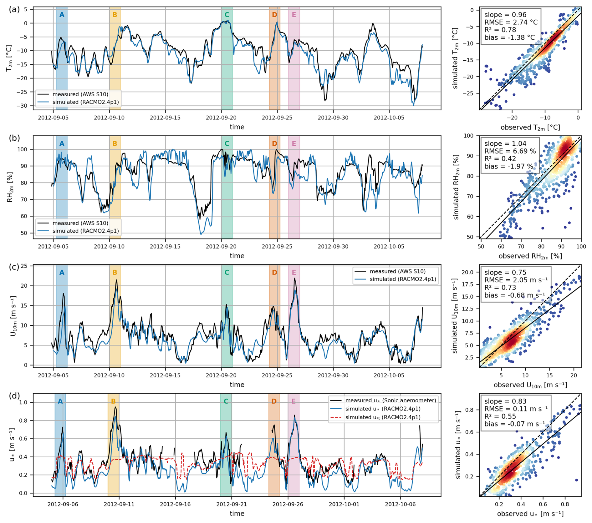
Figure B1 Timeseries and scatter plots of measured and simulated input variables of PIEKTUK-D from RACMO2.4p1 at site S10 from 7 September 2012 until 6 October 2012: (a) 2 m temperature T_2 m [°C], (b) 2 m relative humidity RH_2 m [%], (c) 10 m horizontal wind speed U_10 m [m s⁻¹], (d) friction velocity u_* [m s⁻¹] including the simulated threshold friction velocity u_*t [m s⁻¹] in red. Dashed lines represent the 1:1 line, solid lines represent the best-fit line, and the colours represent the normalised point density from low (0.0, dark blue) to high (1.0, red).

Appendix C: Evaluation of the blowing snow model PIEKTUK-D

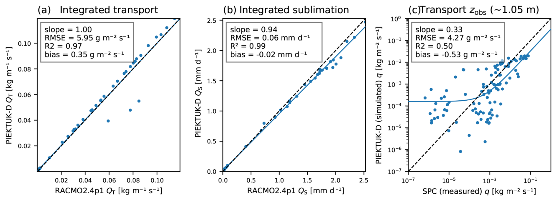
Figure C1 Scatter plots of the measured and simulated horizontal blowing snow transport fluxes and sublimation rates at site S10 from 7 September 2012 until 6 October 2012 for RACMO2.4p1 and the offline PIEKTUK-D model: (a, b) vertically integrated horizontal blowing snow transport flux Q_T [$\mathrm{kg}{\mathrm{m}}^{-\mathrm{1}}{\mathrm{s}}^{-\mathrm{1}}$] and vertically integrated sublimation rate Q_S [mm d⁻¹] of RACMO2.4p1 and PIEKTUK-D (including blowing snow grid and mean radius bugs), and c) measured and simulated horizontal blowing snow transport fluxes q [$\mathrm{kg}{\mathrm{m}}^{-\mathrm{2}}{\mathrm{s}}^{-\mathrm{1}}$] of the SPC and PIEKTUK-D at the observation height above the surface z_obs (without bugs). Dashed lines represent the 1:1 line, solid lines represent the best-fit line, and the colours represent the normalised point density from low (0.0, dark blue) to high (1.0, red).

Appendix D: Evaluation of the radiation model ecRad-1.4.1

Figure D1 Density scatter plots of the simulated surface radiation fluxes at site S10 for RACMO2.4p1 and the offline baseline model: (a) downwelling surface shortwave radiation flux SW_↓ [W m⁻²], (b) upwelling surface shortwave radiation flux SW_↑ [W m⁻²], (c) downwelling surface longwave radiation flux LW_↓ [W m⁻²], and (d) upwelling surface longwave radiation flux LW_↑ [W m⁻²]. Dashed lines represent the 1:1 line, solid lines represent the best-fit line, and the colours represent the normalised point density from low (0.0, dark blue) to high (1.0, red).