Relationships between Arctic sea-ice concentration, temperature, and specific humidity in the lower troposphere during 1980–2021

Understanding of the local effects of sea-ice concentration (SIC) variations on the Arctic atmosphere is a prerequisite for assessing the role of Arctic sea-ice decline in the climate system, including its influence on mid-latitudes. In this study, we analysed the relationships between SIC and both temperature and specific humidity at the surface and 2 m level, as well as at 950, 850, 750, and 600 hPa across the circumpolar Arctic. The role of wind speed and direction in the relationships between SIC and both temperature and specific humidity is discussed. We applied linear ordinary-least-square-regression analysis to detrended anomalies of monthly means of data from the NCEP/CFSR atmospheric reanalysis for 1980–2021. The results show the strongest correlations between SIC and temperature, as well as between SIC and specific humidity, in the marginal ice zone during the cold seasons (November–April) with the coefficient of determination (R²) around 0.6 at the surface and near-surface levels and around 0.3 at 950 and 850 hPa. We interpret the statistical results for these cold seasons so that SIC affects air temperature and specific humidity, while the effects of air temperature variations are limited. SIC correlates somewhat better with specific humidity than with temperature, which can be attributed to the exponential dependence of saturation specific humidity on temperature. In the Central Arctic, physical conditions are favourable for high R² values, but low variability in SIC reduces the correlations. In contrast, in regions such as the northern Barents Sea, increased November–April SIC variability from 1980–2000 to 2001–2021 strengthens the correlations, even though previous studies showed that surface heat and moisture fluxes become less sensitive to SIC in a warming climate. This finding suggests that statistical effects can outweigh the physical sensitivity in shaping observed relationships. During the warm seasons (May–October), high enough air temperatures reduce SIC via melting, while the effect of SIC on air temperature and specific humidity cannot be large, as the surface temperature of the sea ice is very close to that of the open ocean. The relationships between SIC and both temperature and specific humidity are generally weaker during these warm seasons with R² at the surface and near-surface levels around 0.4 over the marginal ice zone during May–July and across the entire sea-ice zone during August–October.

1 Introduction

Dynamic and thermodynamic interactions among the ocean, sea ice, snow cover, and atmosphere are fundamental to the Arctic climate system and its ongoing change (Serreze and Barry, 2011; Haapala et al., 2026). The ocean stores a vast amount of heat, but over much of the Arctic Ocean and adjacent seas, this reservoir is largely insulated from the atmosphere by sea ice and the overlying snow pack. Because both sea ice and, in particular, snow have low thermal conductivity, the conductive heat flux from the ocean through the ice–snow column to the surface is generally small, typically on the order of only a few to a few tens of W m⁻² (Persson et al., 2002). Consequently, leads, polynyas, and other areas of reduced sea-ice concentration (SIC) provide important pathways for oceanic heat and moisture to be transferred to the atmosphere, influencing atmospheric stability, temperature, humidity, and cloud formation. Conversely, atmospheric forcing of sea-ice drift and deformation by winds is a primary mechanism for the formation and evolution of leads and other regions of reduced SIC (Valkonen et al., 2021; Aue et al., 2022).

For most of the year, the near-surface air over the ice-covered Arctic Ocean and adjacent seas is much colder than the open leads, which have surface temperatures very close to the freezing point of seawater (−1.6 to −1.8 °C, Wang et al., 2022). During the summer melt season, the open sea, sea ice, and air are close to isothermal. Hence, outside of the melting season, large upward surface fluxes of sensible and latent heat are observed over leads (Andreas et al., 1979). The magnitude of the fluxes depends on (1) the vertical gradients of potential temperature and specific humidity over the leads, (2) the near-surface wind speed, (3) the surface roughness lengths for momentum, heat, and moisture (Andreas, 1987; Gryschka et al., 2023, the latter including effects of flow edges), and (4) stratification of the near-surface air (e.g. Michaelis et al., 2021).

The upward fluxes of sensible and latent heat cause warming and moistening of the near-surface air. The local effects over individual leads have been addressed by observations (Andreas and Cash, 1999) and large-eddy simulations (Weinbrecht and Raasch, 2001; Zulauf and Krueger, 2003). A lead with a width of approximately 0.5 km typically increases the 2 m temperature of the overflying air by 0.5–2 K (Ruffieux et al., 1995; Pinto et al., 2003). Considering the key processes, the temperature increase in a certain air layer over the lead surface depends on the net effect of vertical convergence of sensible heat flux within the air layer and the horizontal cold-air advection from the ice-covered region, acting against the temperature increase. The vertical distribution of heat depends on the magnitude of sensible heat flux and the stratification against which the heat plume must work over the lead (Lüpkes et al., 2012). The situation is analogous for the air specific humidity, except that the increase driven by surface evaporation is usually partly compensated by condensation to sea smoke droplets, typically occurring over winter leads.

Regional effects of SIC on air temperature and specific humidity are more complex, as airmasses experience alternation of warming over leads and cooling over downwind sea ice. Considering processes affecting the vertical distribution of heat and moisture, decrease in SIC reduces the regional stratification (Jun et al., 2016; Gryschka et al., 2023) and typically increases the near-surface wind speed (Mioduszewski et al., 2018; Jakobson et al., 2019), both enhancing vertical mixing. The regional effects of SIC have been studied on the basis of observations using a research aircraft (Brümmer and Thiemann, 2002; Michaelis et al., 2022), a helicopter-borne measuring system Helipod (Bange et al., 2002), vertical profile data from upwind and downwind sides of the study area (Raddatz et al., 2013), as well as satellite remote sensing and atmospheric reanalysis products (Tetzlaff et al., 2013). Further, the regional effects of SIC have been modelled via idealised experiments (Vihma, 1995), large-eddy simulations (Glendening and Burk, 1992; Gryschka et al., 2023), regional high-resolution numerical weather prediction models (Parker et al., 2022), and regional atmospheric climate models (Rinke et al., 2006; Screen and Simmonds, 2013; Liang et al., 2021).

However, except for climate model experiments (e.g. Kay et al., 2011; Naakka et al., 2025), only a few decadal-scale circumpolar studies have explicitly examined how SIC affects Arctic surface and air temperature and specific humidity. This is a knowledge gap, as understanding of the regional effects of SIC variations on the Arctic atmosphere is a prerequisite for assessing the role of Arctic sea-ice decline in the climate system (Döscher et al., 2014; Holland and Hunke, 2022; Taylor et al., 2018), including its influence on mid-latitudes (e.g. Petoukhov and Semenov, 2010; Francis and Vavrus, 2012; Screen and Simmonds, 2013; Vihma, 2014; Yu et al., 2024). Additional knowledge gaps include the following: (1) seasonal and regional differences in the air temperature and specific humidity responses to changes in SIC have not been systematically studied, (2) previous studies on the vertical profile of the response of air temperature and specific humidity to changes in SIC have so far been limited to the atmospheric boundary layer, and (3) although it is well known that the effects of SIC on air temperature and specific humidity are closely associated (Kim et al., 2016), we are not aware of studies quantitatively comparing the sensitivity of air temperature and specific humidity to SIC. The knowledge gaps are topical, as evaporation from the Arctic Ocean and adjacent seas is increasing in response to sea-ice loss (Boisvert and Stroeve, 2015; Boisvert et al., 2015; Boisvert et al., 2023), which further increases the water vapor feedback and cloud cover.

In this study we contribute to filling the above-mentioned knowledge gaps by analysing the relationships between SIC and temperature as well as SIC and specific humidity in the circumpolar Arctic based on reanalysis data from 1980 to 2021. Attention is paid to the relationships at the surface and 2 m level, as well as the levels of 950, 850, 750, and 600 hPa. The analyses build on Uhlíková et al. (2024), which focused on the effects of SIC on sensible and latent heat fluxes, which are a prerequisite for the effects on air temperature and humidity. The analyses cover the effects of decadal changes and, based on detrended data, month-to-month variations in four seasons. The statistical findings are interpreted in the light of physical processes.

2 Material and Methods

In remote regions with sparse observation network, such as our study region in the marine Arctic, atmospheric reanalyses are widely regarded as providing the best available estimate of past states of the atmosphere. Reanalyses combine observations with short-range weather forecasts through a consistent data assimilation framework, using a fixed model configuration and analysis system over multi-decadal periods.

However, atmospheric reanalyses are not free of errors and weaknesses. Under stably-stratified conditions, models often mix the lowermost troposphere too strongly, underestimating near-surface temperature inversions. Hence, under weak winds, reanalyses often produce warm biases near the surface. In addition to challenges in representation of the stable boundary layer, biases are often related to poorly presented or entirely lacking snow pack on top of sea ice (Zampieri et al., 2023). The turbulent and radiative surface fluxes also include uncertainties, reflected for example in a large scatter in their sensitivities to SIC among various reanalyses (Uhlíková et al., 2024, Uhlíková et al., 2025). Furthermore, problems are often related to cloud cover and radiative properties (Huang et al., 2017). SIC, mostly based on assimilation of satellite passive microwave data, also includes uncertainties (Valkonen et al., 2008), and there may be inconsistencies between atmospheric and oceanic variables.

Despite of the errors and uncertainties, reanalyses provide benefits that are not provided by any observational-only dataset, namely spatially complete and temporally continuous fields at regular time intervals and near-uniform spatial resolution across the globe. These characteristics make them particularly well suited for investigating large-scale atmospheric variability and long-term climatological changes, as in our study.

In the present study, we utilised data from one of the major and commonly used atmospheric reanalysis provided by the National Center for Environmental Prediction (NCEP) – Climate Forecast System Reanalysis (CFSR) (Saha et al., 2010, Saha et al., 2011). The term “NCEP/CFSR” in this study refers to data from both NCEP CFSR (covering the period until 2010) and NCEP Climate Forecast System Version 2 (CFSv2; covering the period 2011 onwards). The model updates in CFSv2 compared to previous CFSR primarily affected cloud processes, radiative transfer, and the land surface model (Saha et al., 2014). Changes to the land surface model are not expected to influence our results. While modifications to cloud and radiative transfer parameterizations have potential to affect snow and ice surface temperatures, and therefore the temperature contrast between open water and sea ice, our analyses indicate that their impact is minimal in the marine Arctic, as no systematic differences were detected across the pre- and post-2011 periods (Figs. 2, S1–S3). NCEP/CFSR appears to be the most realistic reanalysis in terms of physical processes of air-sea-ice interactions due to its modelled sea-ice thickness and snow on top of sea ice (Uhlíková et al., 2024) and performed the best in the comparisons against observations with respect to near-surface variables over ice-covered oceans (Jakobson et al., 2012; Tastula et al., 2013; Lindsay et al., 2014). Although CFSR and CFSv2 are not free of biases, they remain well suited for studies where SIC and sea-ice thickness, as well as near-surface air temperature and specific humidity, are critical. Alternatives such as MERRA-2 and ERA5 exhibit important shortcomings, including unphysical features (Sedlar et al., 2012) and warm biases over sea ice (Batrak and Müller, 2019). Although ERA5 has shown superior performance in some regions (Graham et al., 2019), comparative studies have not demonstrated an overall advantage over CFSR and CFSv2 for representing SIC-related processes (Kong et al., 2022). Given our focus on SIC effects, we therefore selected CFSR and CFSv2 for the analyses in this study.

We worked on data with spatial resolution of 0.5° × 0.5° at which both CFSR and CFSv2 outputs are available. We used data from the era of satellite measurements (after 1979) as, compared to previous years, they provide more reliable and consistent information on the concentration of Arctic sea ice, as well as on the vertical profiles of air temperature and specific humidity (Groves and Francis, 2002). In addition to the direct benefits of satellite data assimilation on the profiles, their accuracy close to the sea surface is also improved by better data on SIC. We divided the past 42 years into two 21-year study periods: 1980–2000 and 2001–2021, with the second period representing warmer climate. Furthermore, we divided each year into four seasons with regard to the annual cycle of the Arctic sea ice: (1) November–December–January, (2) February–March–April, (3) May–June–July, (4) August–September–October, where February–March–April represented months preceding and following the maximum sea-ice extent in March, August–September–October months surrounding the month of minimum sea-ice extent in September, and November–December–January and May–June–July represented the transitional seasons.

We used the following variables from NCEP/CFSR: sea-ice concentration (SIC), air temperature at the height of 2 m (T2m) and at the pressure levels of 950, 850, 750, and 600 hPa (T950, T850, T750, and T600) as well as air specific humidity at the height of 2 m (Q2m) and at the pressure levels of 950, 850, 750, and 600 hPa (Q950, Q850, Q750, and Q600). Furthermore, we utilised the snow/ice/ocean surface temperature (Ts) to compute the specific humidity at the (saturated) surface (Qs) according to Launiainen and Vihma (1990). We applied daily means of data calculated from the original temporal resolution of 6 h.

Using the above-listed variables, we studied bilateral relationships between SIC and temperature as well as SIC and specific humidity through coefficients of determination (R²) from ordinary-least-squares-regression analyses (OLSR). For these analyses, we removed intraseasonal and decadal trends and worked with detrended anomalies of SIC, temperature, and specific humidity. Because all variables in reanalyses include uncertainties and this method assumes no uncertainty in the independent variable (in our case SIC), orthogonal-distance regression (ODR; Boggs et al., 1988) appears as more optimal method for the analyses. However, we performed a comparison study of bilateral ODR and OLSR outputs using data from NCEP/CFSR and noted that, while the values of slopes of the regression line varied considerably between the methods, the coefficients of determination were nearly identical (at least to five decimal points). Based on these findings, we decided to utilise OLSR analyses when only studying R², as this regression method requires much less computing resources to perform. We used linear model for the OLSR as we evaluated it as the most applicable for our purposes primarily following from the finding that typically the first order i.e. linear term dominates over higher order ones when describing the relationship between two variables with the Taylor series. To test statistical significance of the coefficients of determination for the fields, we used p-value < 0.05 adjusted by α_FDR=0.10 (false discovery rate, according to Wilks, 2016) to test the null-hypothesis that the time series are independent.

3 Results

3.1 Spatial and temporal variations and trends in sea-ice concentration, temperature, and specific humidity

To illustrate the interannual variability in SIC, surface and air temperature as well as surface and air specific humidity during 1980–2021, we divided the daily means of data into four seasons and calculated annual mean values from this data within each season (hereafter referred to as “seasonal means”) spatially averaged across eight Arctic basins (displayed in Fig. 1). To obtain decadal trends in SIC, temperature, and specific humidity over these Arctic basins during each season, we calculated slopes of OLSR lines of the area-averaged variables using time as an independent variable. Furthermore, also using OLSR and removing the trends within the period 1980–2021, we calculated coefficients of determination between SIC and temperature as well as SIC and specific humidity at the surface, and atmospheric levels of 2 m, 950, 850, 750, and 600 hPa. For all the above-mentioned analyses, we utilised the NCEP/CFSR land-sea mask and only considered grid cells completely covered by the sea.

As displayed in Tables 1, S1, S3, and S5, we found a decreasing decadal trend in SIC over the period 1980–2021 in most Arctic basins in all seasons. During November–July, the decline was the fastest in the the Kara and Barents seas (around −0.03 per decade), and during August–September–October in the East Siberian and Laptev seas (−0.1 per decade). On the contrary, we found increasing decadal trends in surface and near-surface temperatures and specific humidity over all Arctic basins in all seasons: during November–July the trends were strongest over the Kara and Barents seas (with an exception of February–March–April in regards to temperature, which was rising fastest over the Central Arctic), and during August–September–October they were strongest over the East Siberian and Laptev seas. Though the areas of fastest sea-ice decline and fastest surface and near-surface warming and moistening coincided, some areas have warmed considerably, even though the decadal changes in SIC were not large. This was for example the case of the Central Arctic during November–April, which only lost about 0.001 SIC per decade, while the surface and near-surface temperatures increased by more than 1 K per decade during the cold seasons. Therefore, the warming was not driven by surface processes and did not lead to ice melt. This is consistent with the fact that, even after a rapid decadal-scale warming, near-surface air temperatures in the Central Arctic during November–April remain well below freezing for most of the time. The smallest decadal changes in surface and near-surface variables occurred during May–June–July for temperature, and February–March–April for specific humidity.

The speed of the warming and moistening of the Arctic atmosphere during 1980–2021 generally decreased with height (Tables 1, S1, S3, and S5), however, the surface temperature was not always warming the fastest (in relation to SIC decline). For example, over the Greenland Sea, temperatures at 950 and 850 hPa were rising faster than surface and near-surface temperatures during all seasons (accompanied by the same pattern in specific humidity during May–October), likely related to circulation changes, potentially with respect to Greenland blocking (Hanna et al., 2022) and cyclone activity (Zhang et al., 2023). The interannual variability of temperature and specific humidity generally decreased with height over all Arctic basins and seasons (see standard errors in Tables 1, S1, S3, S5).

The strength of the relationship (coefficient of determination, R²) between detrended seasonal means of SIC, temperature, and specific humidity over the eight Arctic basins is shown in Tables 2, S2, S4, and S6. During November–April (Tables 2, S2), R² values between SIC and both surface and near-surface temperature and specific humidity were the largest over the Kara and Barents seas (around 0.8), while during August–September–October (Table S6), the values were the largest over the East Siberian and Laptev seas (around 0.8) and during May–June–July (Table S4) over the Hudson Bay (around 0.6). Across all seasons and throughout the Arctic, the values of R² between SIC and surface and air temperature and specific humidity generally decreased with height.

The seasonal means of SIC, temperature, and specific humidity between the surface and 600 hPa over the eight Arctic basins are shown in Figs. 2 and S1–S3, where panel (a) depicts values of temperature (and SIC) and panel (b) specific humidity (and SIC). Next to the typical values of these variables, these figures include information on typical air temperature and specific humidity profiles over the Arctic basins in each season as follows. During November–April (panel a in Figs. 2 and S1) over the Central Arctic, Beaufort, East Siberian, Laptev, and partly Chukchi seas, seasonal means of surface and near-surface temperatures (Ts, T2m) were consistently lower than temperatures at 950, 850, and in most cases also at 750 hPa (with temperature maxima at 850 hPa), indicating prevailing inversion conditions in these regions. Over the Kara, Barents, and Greenland seas and Baffin and Hudson bays, however, the seasonal means of temperatures generally decreased with height during these cold seasons.

The above-described patterns of temperature stratification during months November–December–January were to a large extent followed by the stratification of specific humidity (panel b in Fig. 2), which relates to the dependency of specific humidity on temperature via the saturation water vapor pressure. Though, the patterns in (all) seasonal means of specific humidity were not identical to those of temperature because of the different air mass origins and evolution before reaching each basin, including for example warm but dry air masses from over the continents or loss of moisture via precipitation on the way (Naakka et al., 2019). Over the Beaufort, East Siberian, and Laptev seas, the seasonal means of specific humidity from the surface up to the 750 hPa level were very similar to each other during February–March–April (panel b in Fig. S1) as they were all very low (around 0.5 g kg⁻¹).

The May–June–July seasonal means of temperature at 950 hPa were the highest over most of Arctic basins (panel a in Fig. S2), reflecting the effect of still mostly high SIC, which decreased the surface and near-surface temperatures. During late summer (August–September–October, panel a in Fig. S3), surface and near-surface temperatures were the highest and temperatures aloft further decreased with height. The above-mentioned pattern for the warm seasons, however, was not seen in seasonal means of specific humidity, which decreased with height over all Arctic basins during both May–June–July and August–September–October (panel b in Figs. S2, S3).

Figures 2 and S1–S3 further depict the coexistence of opposite interannual anomalies in SIC and temperature or specific humidity, which agreed with the strength of the above-described coefficients of determination between the variables. Among the most striking interannual anomalies were, for example, those during August–September–October 2007 over the Chukchi, East Siberian, and Laptev seas (Fig. S3), with positive interannual anomalies in temperature and specific humidity (around +4.5 K for Ts and T2m and around +1 g kg⁻¹ in Qs and Q2m) accompanied by negative interannual anomalies in SIC (around −0.3). The positive anomalies in temperature and specific humidity decreased with height during August–September-October, while during the preceding season of May–June–July (Fig. S2), we found the maximum values of positive interannual anomalies at 850 hPa (around +2.5 K and +0.5 g kg⁻¹, reflected in −0.1 anomalies in SIC).

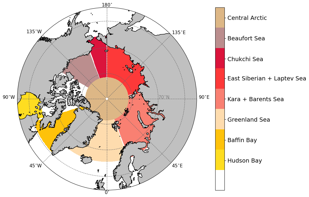
Figure 1 Arctic basins used for calculating areal seasonal means of sea-ice concentration, temperature, and specific humidity, their decadal trends, and correlation coefficients in Tables 1, 2, S1–S6, and Figs. 2 and S1–S3.

Table 1 Change per 10 years during November–December–January in sea-ice concentration (SIC), temperature at the surface and the levels of 2 m, 950, 850, 750, and 600 hPa (Ts, T2m, T950, T850, T750, T600), and specific humidity at the same levels (Qs, Q2m, Q950, Q850, Q750, Q600) over the eight Arctic basins (as shown in Fig. 1). Changes were calculated from area-averaged annual means (of daily means in November–December–January) during 1980–2021 as slopes of ordinary-least-square-regression line using time as an independent variable. Units of temperature and specific humidity changes are K per 10 years and g kg⁻¹ per 10 years, respectively. Statistically significant results at the confidence level p<0.05 are marked in bold. Standard errors of the slopes are marked in italics.

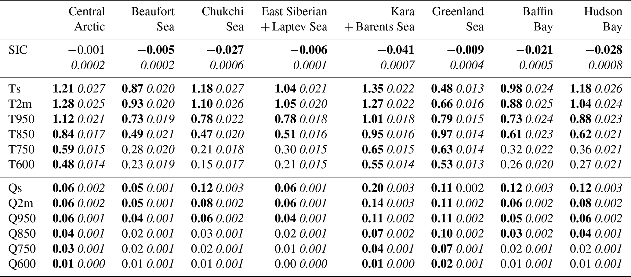
Table 2 Coefficient of determination (R²) between detrended seasonal means (calculated from daily means) of sea-ice concentration (SIC) and temperature at the surface and the levels of 2 m, 950, 850, 750, and 600 hPa (Ts, T2m, T950, T850, T750, T600), and specific humidity at the same levels (Qs, Q2m, Q950, Q850, Q750, Q600) over the areas of eight Arctic basins (as shown in Fig. 1) for November–December–January during 1980–2021. Statistically significant results at the confidence level p<0.05 are marked in bold.

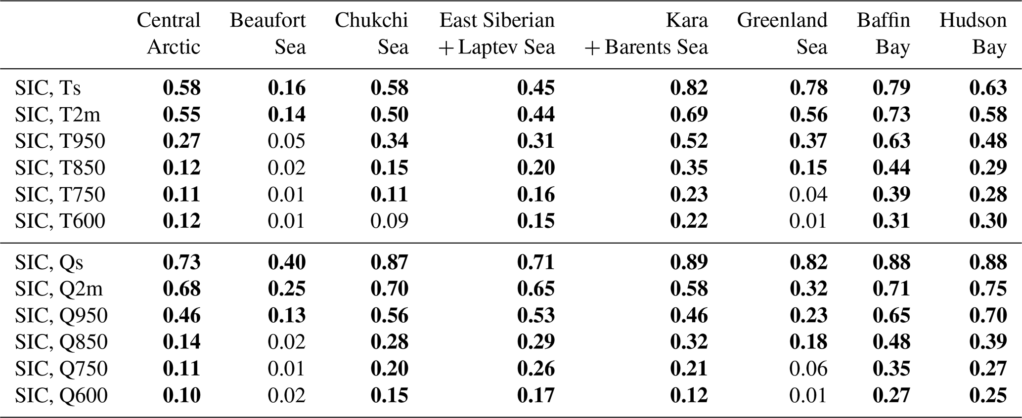
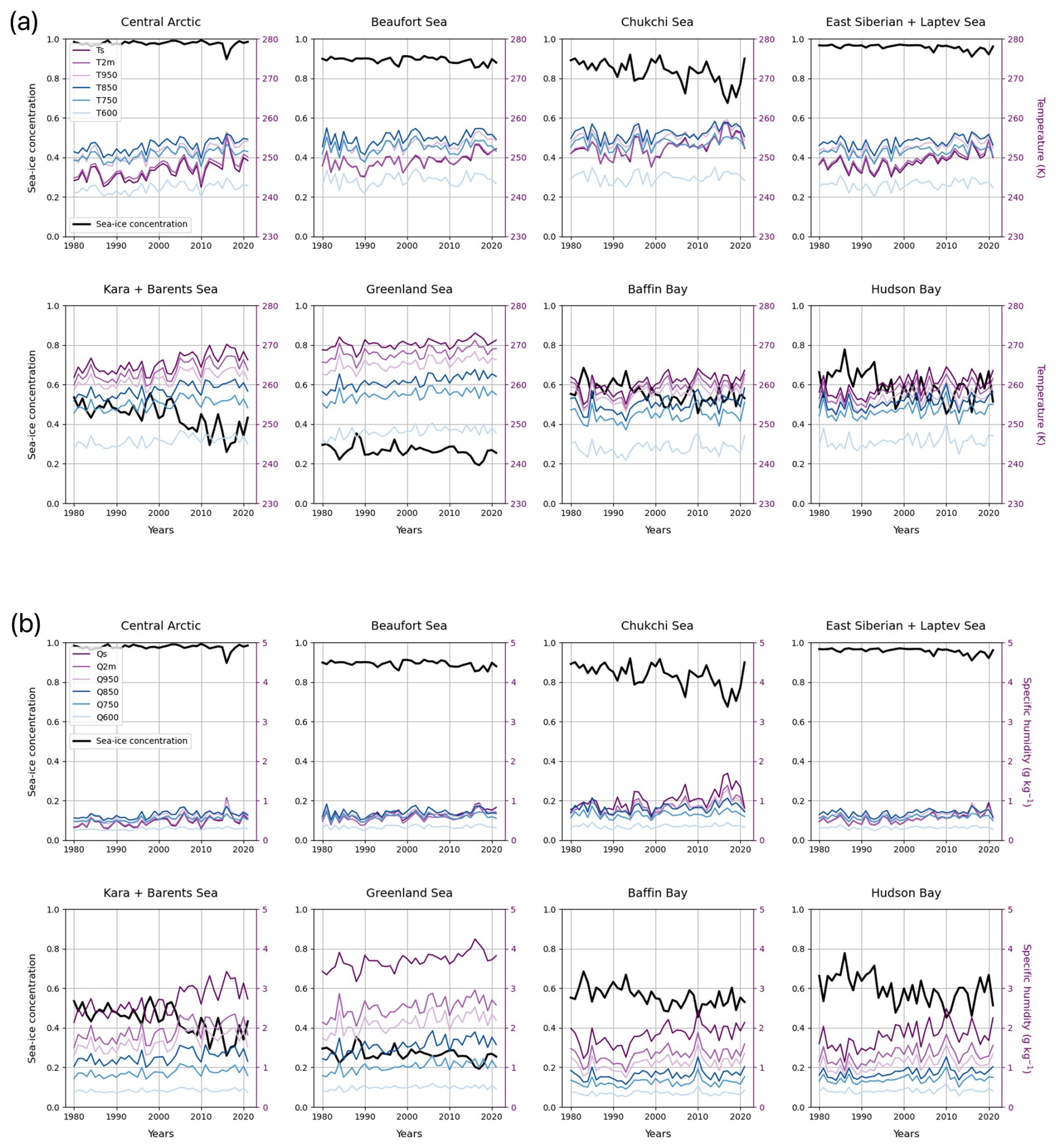
Figure 2 Seasonal means calculated from daily means in November–December–January (months within the same year) during years 1980–2021 averaged over the areas of eight Arctic basins (as shown in Fig. 1). (a) Sea-ice concentration and temperature at the surface and the levels of 2 m, 950, 850, 750, and 600 hPa (Ts, T2m, T950, T850, T750, T600). (b) Same as (a) but for the surface and air specific humidities. Only grid cells fully covered by the sea were considered in this analysis.

3.2 Relationships of sea-ice concentration, temperature, and specific humidity

When examining mean seasonal and decadal values of SIC, temperature, and specific humidity, a substantial amount of information about their true variability is lost. On the other hand, using daily mean values includes a lot of synoptic-scale variability in air temperature and humidity, not driven by SIC but by weather events.

Hence, in this subsection, we base the analyses on monthly mean data (calculated from daily means), and perform linear bilateral OLSR analyses of SIC and temperature as well as SIC and specific humidity at the surface and the levels of 2 m, 950, and 850 hPa. For these analyses, we removed the intraseasonal and decadal trends (within each month and the study periods 1980–2000 and 2001–2021).

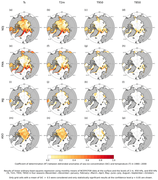
Coefficients of determination between monthly SIC and temperature in all seasons during 1980–2000 are depicted in Fig. 3. We observed the strongest relationship between SIC and surface and near-surface temperature during November–April (R² around 0.3 over the inner ice pack and around 0.6 over the marginal ice zones; panels a, b, e, f in Fig. 3) and during August–October (around 0.4 throughout the ice pack, panels m, n in Fig. 3). The drivers and strength of the relationships between SIC and temperature or vice versa depend on season and region and in the above-mentioned seasons with the strongest relationships between the variables are the following: (1) In early winter (November–December–January), positive anomalies in near-surface temperature may have a large effect on the sea ice over most of the Arctic through reduction of the freezing rate. At the same time, leads and polynyas in the sea-ice pack created by divergent ice drift or anomalous oceanic heat flux contribute to raising the air temperature by releasing heat from the underlying ocean. (2) The sea ice is the thickest during late winter (February–March–April) and the near-surface temperatures are usually below zero. Hence, in general, even positive anomalies in near-surface temperatures do not decrease SIC during this season, however, they favour slower refreezing of open leads (and eventual polynyas). At the same time, SIC in the inner ice pack is very high and does not vary much, so the strength of the relationship with air temperature in these areas is limited (panels e, f of Fig. 3). (3) During late summer (August–September–October) on average, there is just a small difference between the temperature of the ocean at seawater freezing point (−1.6 to −1.8 °C) and ice surface temperature at about the snow/ice melting point (0 °C), so the presence or absence of sea ice cannot have much effect on surface and near-surface temperature (Lüpkes et al., 2010). On the contrary, positive monthly anomalies in surface and near-surface temperatures have potential for detectable effects and are indeed associated with negative anomalies in SIC. Panels (m), (n) of Fig. 3 depicting the late summer conditions include October, when the air is already colder than the water, but the nearly isothermal conditions in August and September probably dominate the plots. Elevated air temperatures are associated with low SIC also during May–June–July, however, we observed the effect mostly over coastal seas (panels i, j of Fig. 3). This can be explained as the air over the continents nearby is already warm, especially during June and July, and when advected over the sea ice, it causes negative SIC anomalies. However, air masses cool with fetch over the ice, and air masses originating from over the ocean or Greenland ice sheet are considerably colder than those originating from continents in summer.

As expected, in all seasons, the coefficients of determination between SIC and temperature weakened with height. During the cold seasons November–April, the R² values between SIC and air temperature over the marginal ice zones were around 0.3 at the 950 hPa level and around 0.2 over limited areas at the 850 hPa level, while we found no significant relationship at these levels over the inner ice pack (panels c, d, g, h of Fig. 3). This may be connected to the atmospheric stratification that is stable or very stable over the areas of high SIC (as shown e.g. in Persson et al., 2002), which usually prevents the warming and moistening effects of open leads from reaching high altitudes (Michaelis et al., 2022). Accordingly, large-scale circulation has a more dominating effect on temperature and specific humidity aloft, because the surface forcing, that may either support or oppose the large-scale forcing, does not reach these higher altitudes during the cold seasons.

The relationship between SIC and specific humidity generally followed similar patterns to that between SIC and temperature, but with consistently higher coefficients of determination by about 0.1–0.2 across all seasons and most altitudes (Fig. 4). We examined whether this difference can be explained by the exponential dependence of saturation specific humidity on temperature. Hudson Bay stood out as one of the regions where the R² between SIC and Q2m was markedly higher than that between SIC and T2m during November–December–January 1980–2000 (panel b of Figs. 3, 4). Monthly mean values of SIC and T2m, and SIC and Q2m from a grid cell nearest to 60° N and 90° W from this season and study period are shown in panels (a), (b) of Fig. 5. The SIC, Q2m relationship (R²=0.91) is closer to linear than the SIC, T2m relationship (R²=0.85). In the latter, T2m declines sharply as SIC approaches unity. This reflects the fact that, due to the strong insulation by ice and snow, a compact winter ice cover is typically associated with very low near-surface air temperatures. When small leads open, even a slight reduction in SIC (e.g., from 1.00 to 0.99) can produce intense fluxes of sensible and latent heat from the open water (Uhlíková et al., 2024), causing T2m and Q2m to respond strongly. This behaviour for near-surface air temperature was demonstrated in model experiments by Lüpkes et al. (2008), whose results closely match our panel (a) in Fig. 5, showing a concave-down SIC, T2m dependence (see also their Fig. 4). Less attention has been paid on the Q2m response to SIC changes. However, although the latent heat fluxes over leads are typically smaller than the sensible heat fluxes, particularly in cold seasons, also the former are very sensitive to SIC (Uhlíková et al., 2024). This is at least partly due to the fact that the surface saturation specific humidity increases exponentially with temperature and, accordingly, in cold seasons the relative difference in surface saturation specific humidity between open leads and sea ice is larger than that in surface temperature.

According to Andreas et al. (2002), the near-surface air over polar sea ice is always close to saturation with respect to ice. Assuming this holds for the Hudson Bay, we used T2m data from NCEP/CFSR to calculate ice-saturated water vapour pressure E_s according to Buck (1981):

$$\begin{array}{}\text{(1)}& E_{\mathrm{s}}=\left(\mathrm{1.0003}+\mathrm{4.18}\times {\mathrm{10}}^{-\mathrm{6}}p\right)\mathrm{6.115}{\mathrm{e}}^{\frac{\mathrm{22.452}T\mathrm{2}m}{\mathrm{272.55}+T\mathrm{2}m}}\end{array}$$

where p is the mean-sea-level pressure (in hPa) and T2m is in degrees Celsius. Then the ice-saturated 2 m specific humidity (Q2m_SAT) was calculated as:

$$\begin{array}{}\text{(2)}& \mathrm{Q}\mathrm{2}{\mathrm{m}}_{\mathrm{SAT}}={\displaystyle \frac{\mathrm{0.622}{E}_{\mathrm{s}}}{p-\mathrm{0.378}{E}_{\mathrm{s}}}}\end{array}$$

The dependence of Q2m_SAT on SIC is nearly perfectly linear, with R² of 0.94 (panel c of Fig. 5). This arises because Q2m_SAT increases exponentially with T2m, which in turn is inversely related to SIC; thus, the concave-down SIC, T2m relationship transforms into an almost straight line for the dependence of Q2m_SAT on SIC. The actual SIC, Q2m relationship in the NCEP/CFSR data (panel b of Fig. 5) lies between those of T2m and Q2m_SAT indicating that Q2m in the reanalysis is not always fully saturated with respect to ice. In summary, the exponential dependence of saturation specific humidity on temperature explains why SIC correlates more strongly with Q2m than with T2m. This can be visualised using the original (real) data, as the saturation specific humidity depends on the real air temperature instead of the detrended anomalies.

However, the results presented in Figs. 3 and 4 are based on detrended anomalies of SIC, temperature, and specific humidity, hence, the analyses for the Hudson Bay location must be repeated using these time series. The results (panels d–f in Fig. 5) naturally show much smaller R² values (equal to those in panel b of Figs. 3 and 4) because the data do not include intraseasonal and decadal trends (see Sect. 2). However, the differences between the R² values for SIC and T2m, Q2m, or Q2m_SAT are even larger than those based on the original data (panels a–c in Fig. 5). This suggests that the conclusions made based on the original data remain valid, although the exponential dependence of Q2m_SAT on T2m and the co-occurrence of high SIC and low T2m are not visualized when showing the detrended anomalies of data (panels d–f in Fig. 5).

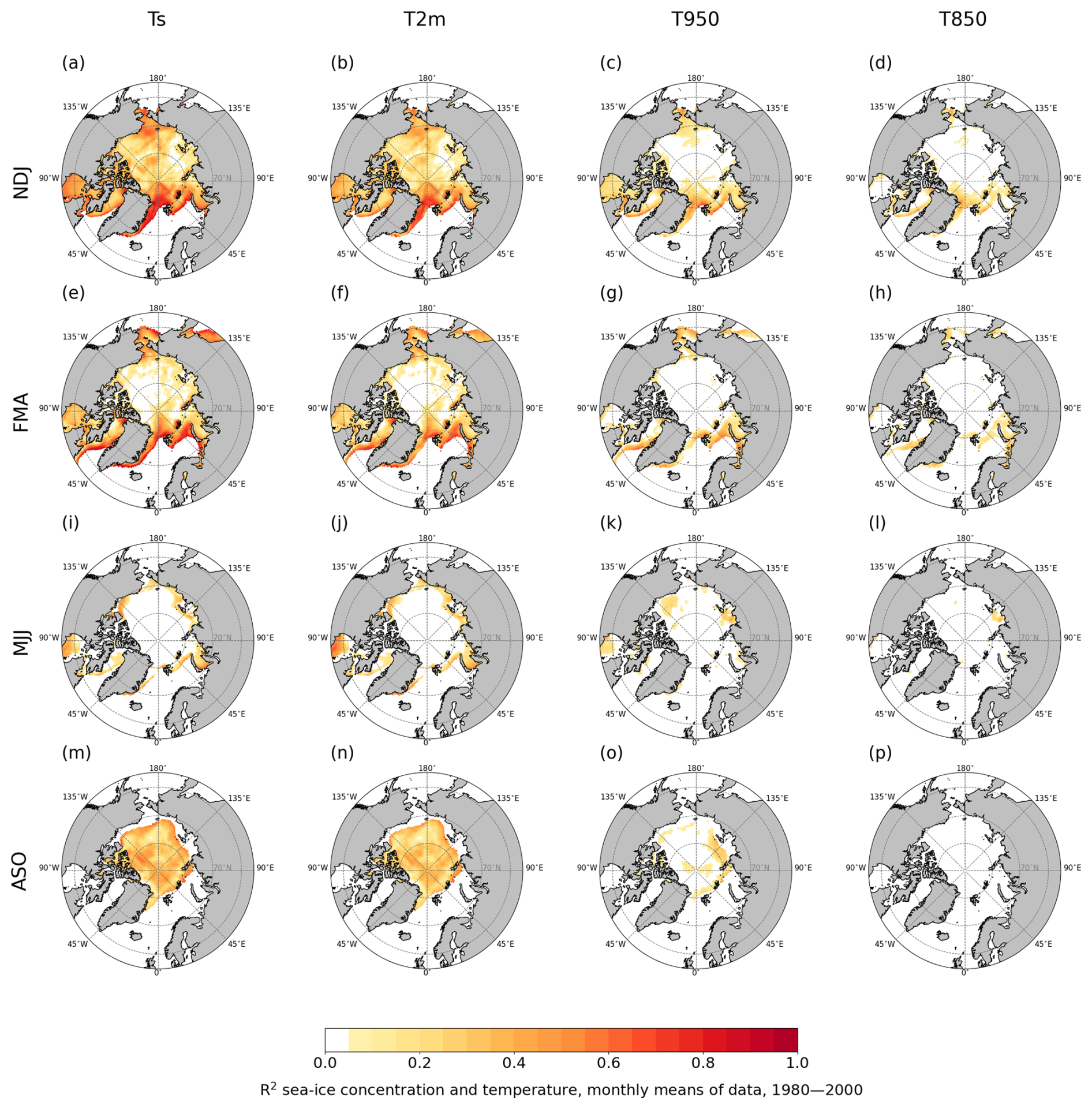
Figure 3 Coefficient of determination (R²) between detrended anomalies of sea-ice concentration and temperature at the surface and the levels of 2 m, 950, and 850 hPa (Ts, T2m, T950, T850) in four seasons (November–December–January, February–March–April, May–June–July, August–September–October) in 1980–2000. The results are based on linear ordinary-least-squares-regression model using monthly means of NCEP/CFSR data. Only grid cells with a mean of SIC > 0.5 were considered and only statistically significant results at the confidence level p<0.05 are shown (insignificant ones are masked in white).

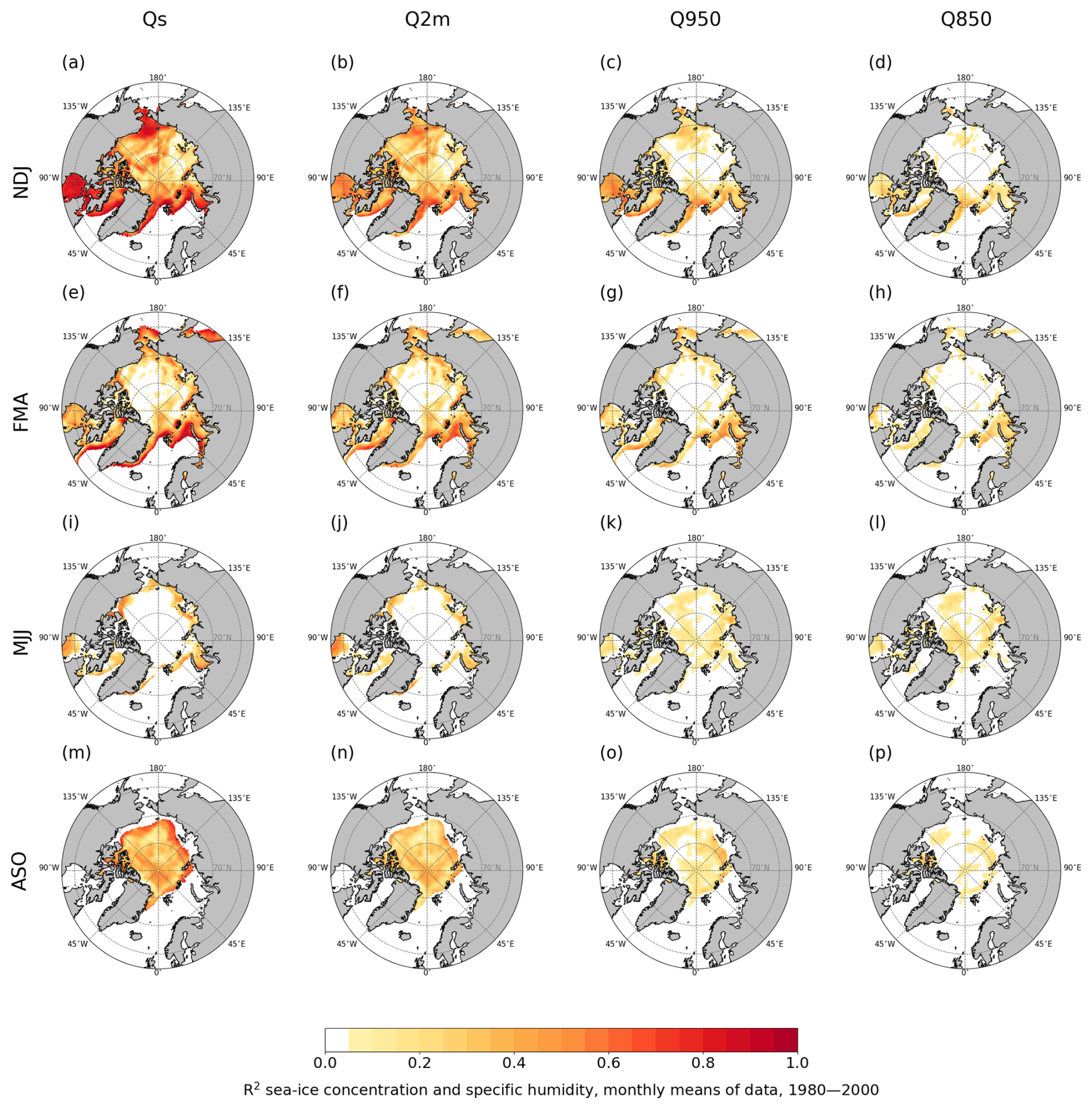
Figure 4 Coefficient of determination (R²) between detrended anomalies of sea-ice concentration and specific humidity at the surface and the levels of 2 m, 950, and 850 hPa (Qs, Q2m, Q950, Q850) in four seasons (November–December–January, February–March–April, May–June–July, August–September–October) in 1980–2000. The results are based on linear ordinary-least-squares-regression model using monthly means of NCEP/CFSR data. Only grid cells with a mean of SIC > 0.5 were considered and only statistically significant results at the confidence level p<0.05 are shown (insignificant ones are masked in white).

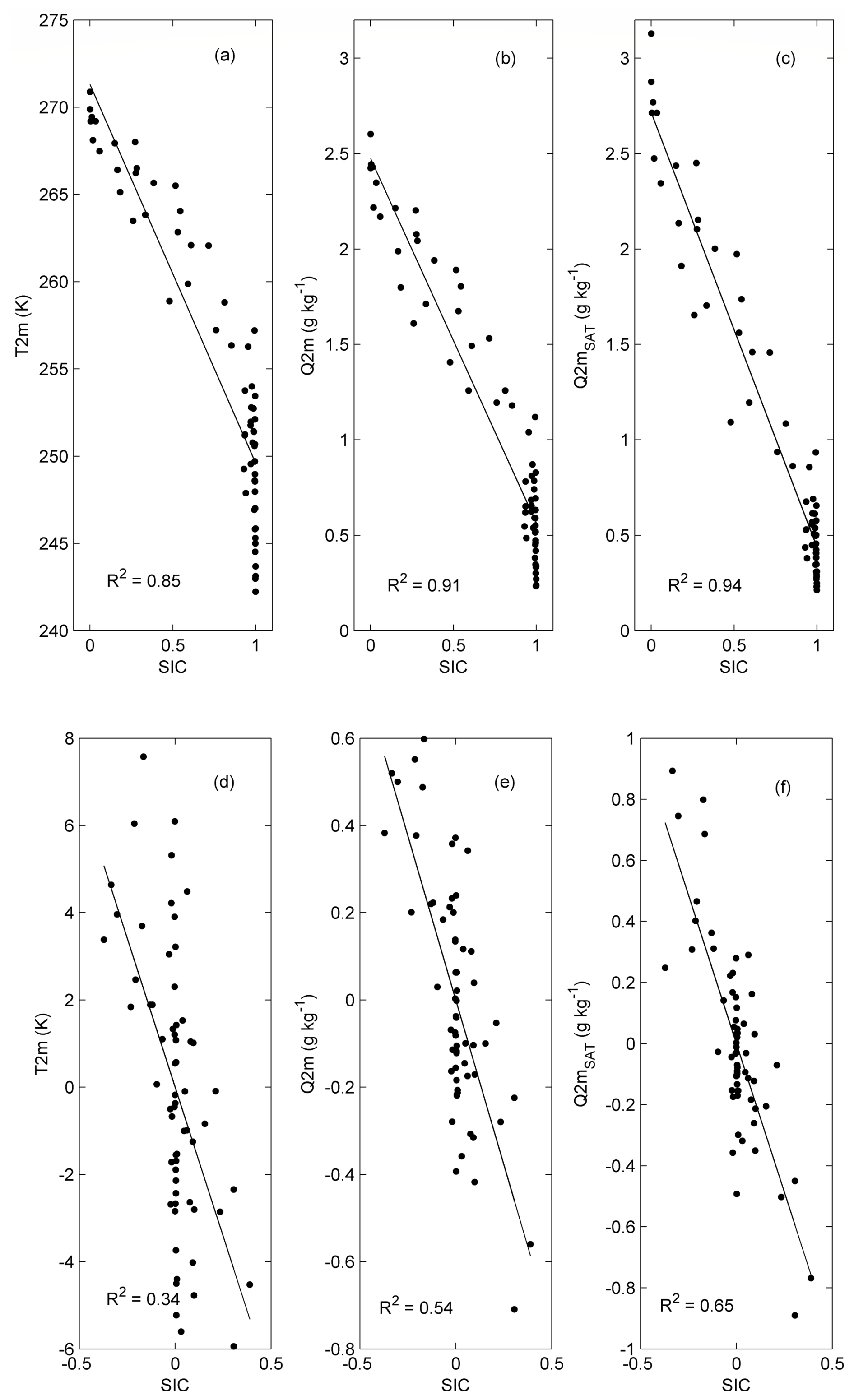
Figure 5 Dependence of (a) 2 m air temperature (T2m), (b) 2 m specific humidity (Q2m), and (c) 2 m saturated specific humidity (Q2m_SAT) on sea-ice concentration (SIC) in the Hudson Bay calculated using Eqs. (1) and (2). Monthly means of NCEP/CFSR data in a grid cell nearest to 60° N and 90° W during November-December-January in 1980–2000. Panels (d), (e), (f) show same as panels (a), (b), (c) but for detrended anomalies of the data.

3.3 Decadal changes in the relationships of sea-ice concentration, temperature, and specific humidity

The values of R² considering detrended anomalies of monthly means of SIC, temperature, and specific humidity at the surface and the levels of 2 m, 950 and 850 hPa during 2001–2021 are depicted in Figs. S4 and S5. Furthermore, the differences in these R² values between the two study periods (1980–2000 and 2001–2021) for SIC and temperature are presented in Fig. 6. We found the highest values and largest areas of the decadal changes in the strength of the relationship between SIC and surface and near-surface temperatures during November–December–January and August–September–October (panels a, b, m, n in Fig. 6). During November–December–January, R² of SIC and temperature decreased over the western part of Fram Strait (Points 1, 4, 7, 10 in Fig. 6), western part of the Central Arctic, and the Beaufort Sea and increased over the northern part of Barents Sea (Points 2, 5, 8, 11 in Fig. 6), Kara and Laptev seas, and eastern part of the Central Arctic (Points 3, 6, 9, 12 in Fig. 6). During August–September–October, the relationship of SIC and temperature weakened over most of the Central Arctic and northern Beaufort Sea (Points 13, 15, 17, 19 in Fig. 6), and strengthened over the northern part of the East Siberian Sea (Points 14, 16, 18, 20 in Fig. 6).

To explore individual monthly values of detrended anomalies of SIC and temperatures (Ts to T850) in the above-indicated areas of interest, where R² decreased or increased considerably between the study periods, we analysed these values over five locations in Fig. 7. Over the western part of Fram Strait, during November–December–January (first column of panel a in Fig. 7), we observed that at all considered atmospheric levels (and at the surface), the variability of temperature remained rather similar in both study periods, while the variability of SIC somewhat decreased in the second study period, causing lower sensitivity of temperature to SIC. The situation over the northern Barents Sea (second column of panel a in Fig. 7) seemed to be opposite from the point of view of SIC, whose variability increased considerably between the study periods, while that of temperatures increased only slightly, still ensuing larger R² between the variables. Over the eastern part of the Central Arctic, during the first study period (black dots in the third column of panel a in Fig. 7), the variability of SIC was very low throughout November–December–January months and therefore the relationships of SIC and temperatures were weak. During the second study period (red dots in the third column of panel a in Fig. 7), there were three months (two Novembers and one January) with higher negative SIC anomalies accompanied by strong positive temperatures anomalies, which increased the R² between the variables.

In August–September–October during 1980–2000, the variability of detrended anomalies of both SIC and temperatures were small over the northern parts of Beaufort and East Siberian seas (black dots in panel b of Fig. 7). In comparison, during 2001–2021 in the northern Beaufort Sea (blue dots in the first column of panel b in Fig. 7), we noted more negative anomalies in SIC, however, these were accompanied by temperature anomalies of a very low magnitude, leading to lower values of coefficients of determination in the second study period. On the contrary, in the northern East Siberian Sea (red dots in the second column of panel b in Fig. 7), the increase in the magnitude of positive temperature anomalies was reflected in a rather strong increase in the magnitude of negative SIC anomalies, rising R² of the variables in the area.

Similarly to the absolute values of R² between SIC and temperature compared to SIC and specific humidity, the decadal differences in R² of specific humidity were qualitatively similar to those of temperature, only about 0.1–0.2 higher (Fig. S6).

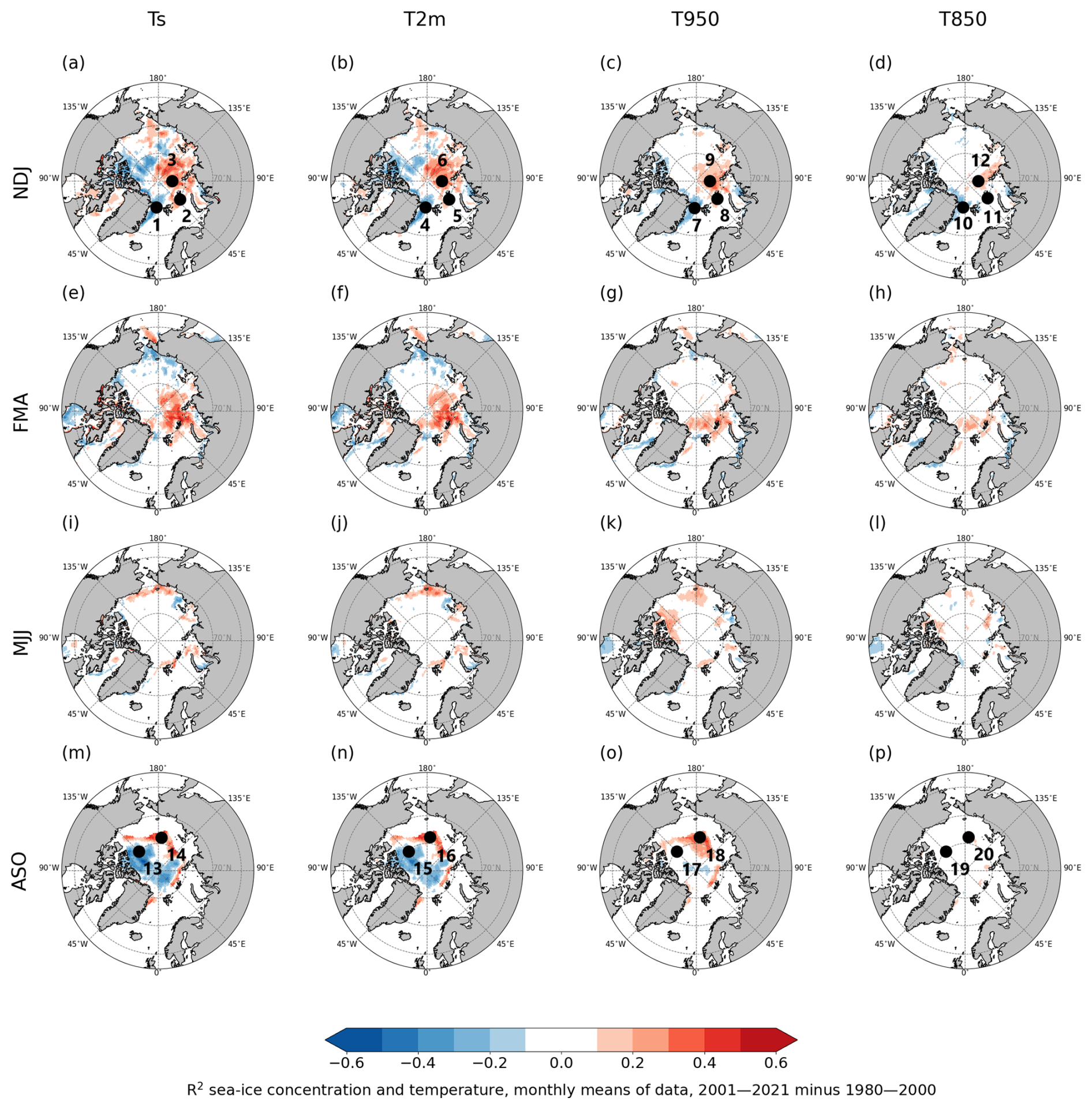
Figure 6 Difference in coefficients of determination (R²) for detrended anomalies of sea-ice concentration and temperature at the surface and the levels of 2 m, 950, and 850 hPa (Ts, T2m, T950, T850) between 1980–2000 and 2001–2021. The results are based on linear ordinary-least-squares-regression model using monthly means of NCEP/CFSR data. Only grid cells with a mean of SIC > 0.5 were considered. Points 1–20 (in black) from panels (a)–(d) and (m)–(p) are further analysed in Fig. 7.

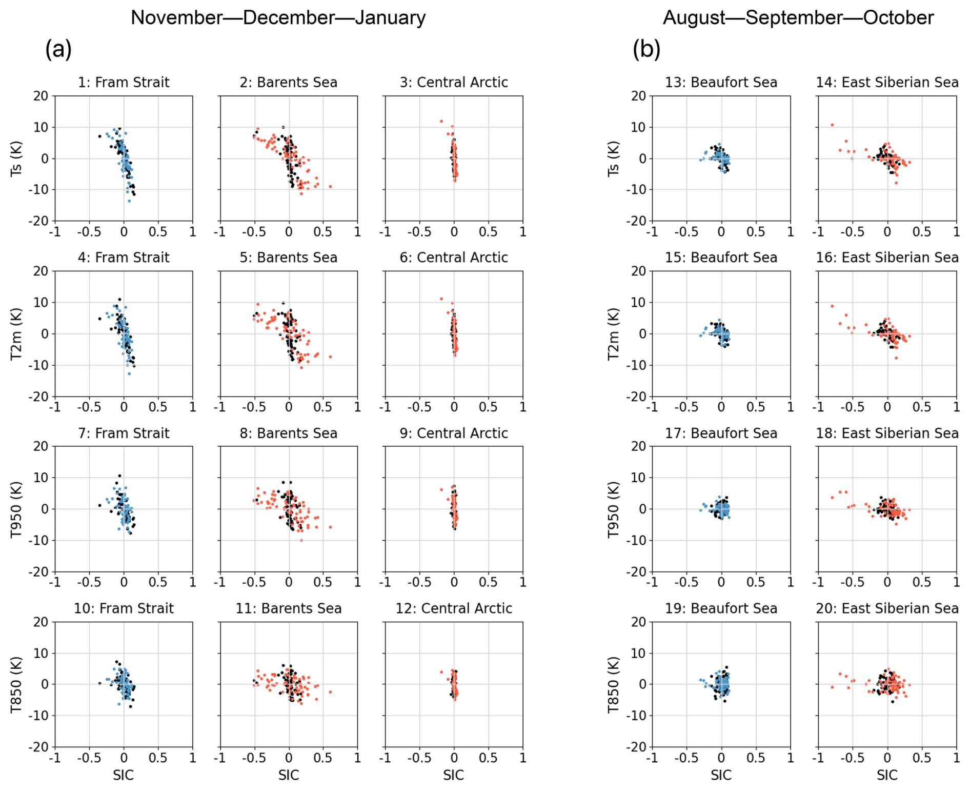
Figure 7 Monthly detrended anomalies of sea-ice concentration (SIC) and temperature at the surface and the levels of 2 m, 950, and 850 hPa (Ts, T2m, T950, T850) in selected grid cells from Fram Strait, Barents Sea, Central Arctic, and Beaufort and East Siberian seas. Data from NCEP/CFSR in months November–December–January are shown in panel (a), and in August–September–October in panel (b). Grid cells 1–20 are indicated in Fig. 6 in panels (a)–(d) and (m)–(p). Values from 1980–2000 are depicted in black. Values from 2001–2021 are depicted in blue in cases when R² between the variables decreased between the study periods, and in red in cases when R² increased.

4 Discussion

4.1 Decadal changes in the variability of sea-ice concentration and temperature

In the Fram Strait during November–December–January, we observed decadal decrease in monthly SIC variability (Points 1, 4, 7, 10 in Figs. 6 and 7) resulting in lower R² between SIC and temperature anomalies in the second study period (2001–2021).

In this region and season, a decadal increase in SIC to almost 1 was seen in atmospheric reanalyses ERA5, MERRA-2, and NCEP/CFSR (Uhlíková et al., 2025). Higher SIC then increased the compactness of the ice field and reduced SIC variability in this season, which logically explains our NCEP/CFSR-based findings. However, combining satellite remote sensing and reanalysis data, Schmitt and Lüpkes (2023) detected predominantly decreasing SIC in the Fram Strait for the winters of 1992 to 2022, while increasing SIC was only observed locally. Such discrepancies may arise from the different processing algorithms applied to derive SIC from satellite passive microwave data (Valkonen et al., 2008).

In the northern Barents Sea during November–December–January (Points 2, 5, 8, 11 in Figs. 6 and 7), the decadal increase of interannual variability of SIC and temperature anomalies (favouring the increase of their coefficient of determination) was likely related to the location becoming part of more dynamic marginal ice zone in the second study period due to general sea-ice decline in the Barents Sea (Onarheim et al., 2018). The possible generation mechanisms of positive and negative SIC anomalies were then described for example in Årthun et al. (2012), who showed the connection of SIC variability in the area to Atlantic heat transport, or Efstathiou et al. (2022), who described the import of sea ice to the area from the north through the gateways of Franz Josef Land–Novaya Zemlya or Svalbard–Franz Josef Land, predominantly driven by northerly and easterly winds. Increased variability in air temperature in the northern Barents Sea during November–December–January may be attributed to two factors: (1) cyclone tracks having become more meridional in the region, with increased cyclone activity in the northern Barents Sea and decreased one in the southeastern Barents Sea (Wickström et al., 2020) and (2) increased SIC variability in the northern Barents Sea as described above.

Similarly to the northern Barents Sea during November–December–January, R² between temperature and SIC anomalies increased during August–September–October over the northern East Siberian Sea in the second study period (Points 14, 16, 18, 20 in Figs. 6 and 7), due to higher variability in both temperature and SIC. This shift likely happened because of the area's transition from the predominantly high SIC conditions towards the marginal ice zone as indicated by Onarheim et al. (2018), who showed that the largest Arctic sea-ice loss since 1979 during September took place in the East Siberian Sea. Additionally, the cyclone activity increased over the northern East Siberian Sea (Kruglova and Myslenkov, 2024), which may have been another driver of the increased temperature variability besides the increased SIC variability.

4.2 Physical and statistical factors

We found somewhat stronger linear relationship between SIC and specific humidity than between SIC and air temperature (Figs. 3, 4, S4, S5). However, this mostly arises from the fact that the sensitivity of air temperature to SIC is strongest when SIC is large and air is cold, making the relationship nonlinear. The exponential dependence of saturation specific humidity compensates for this nonlinearity, yielding a higher linear correlation between SIC and specific humidity. However, the physical linkage is not stronger for specific humidity. Effects of SIC on both air temperature and specific humidity are highly important, as they together control cloud formation and associated effects and feedbacks related to solar (shortwave) and thermal (longwave) radiation in the Arctic climate system.

The dependence of air temperature and specific humidity on SIC is affected by both physical and statistical factors. From the physical point of view, the dependence of T2m and Q2m of SIC is expected to be strong when (1) the air is cold and dry, (2) the lateral advection of heat and moisture is weak, and (3) the atmospheric-boundary-layer stratification is strong. Combination of these conditions allows large turbulent fluxes of sensible and latent heat over leads, which dominate over the advective effects and, due to the strong stratification, heat and moisture originating from leads remains in the atmospheric boundary layer. However, this does not guarantee that SIC has a high R² value with T2m and Q2m. In the Central Arctic during the cold seasons November–April, all three conditions (1 to 3 above) are typically met, but the R² values are generally smaller than further south (panels b, f in Figs. 3, 4). According to our interpretation, this is largely due to a statistical factor: in the Central Arctic during the cold seasons, the variability of SIC is very small (as shown e.g. in panel a of Fig. 7) and therefore the effect of SIC variations on T2m and Q2m is too small to dominate over the variations generated by other factors, the most important ones being the cloud cover, scalar wind speed, and horizontal advection of heat and moisture (Walsh and Chapman, 1998; Vihma and Pirazzini, 2005). These seem to dominate, although during the cold seasons, the sensitivity of near-surface temperature to SIC is highest when SIC is large, i.e. for a 1 percentage point change in SIC, the change of air temperature is largest when SIC is close to 1 (Lüpkes et al., 2008).

The role of statistical factors is evident also via the fact that over certain regions (such as the eastern Central Arctic during November–December–January), R² between SIC and the atmospheric variables increased on a decadal time scale (due to increased SIC variability, panel a in Fig. 7), although the physical factors favoured a decrease. The latter is because during the cold seasons, the surface temperature difference between leads and sea ice decrease with climate warming (the snow/ice surface becomes warmer, but the lead surface remains at −1.6 to −1.8 °C), reducing the sensitivity of sensible and latent heat flux (Uhlíková et al., 2024) and further air temperature and specific humidity to SIC.

4.3 Role of temperature inversions and wind

The occurrence and strength of temperature inversions are very important factors in suppressing the transmission of the surface forcings aloft (mostly during the cold seasons) or preventing the effect of advected warm and moist air masses in reaching the surface. Although events of penetration of heat plumes into mid-troposphere have been observed in the Arctic (Schnell et al., 1989), our results were qualitatively in line with Serreze et al. (1992), who concluded that a deep penetration is a rare event, requiring atypical combination of conditions (leads or polynyas at least 10 km wide, weak surface winds, low surface temperature, and a weak temperature inversion). As in Screen and Simmonds (2010), we found that the direct effects of SIC on the air temperature strongly declined with altitude.

It should be noted that stratification is not the only factor affecting the vertical profile of R² between SIC and air temperature or specific humidity. Another factor is the vertical profile of heat and moisture transport to the Arctic. Northward moisture transport peaks at 900–950 hPa level and the net moisture transport at 800–850 hPa level (Naakka et al., 2019). Hence, the strong role of moisture transport on these levels tends to reduce the correlation between SIC and air moisture at the same levels. In any case, there is a need for more research to quantify the factors controlling the vertical profiles of the relationship of SIC and air temperature or specific humidity.

In the marginal ice zones, wind speed and direction may in some cases simultaneously affect both the SIC, air temperature and specific humidity. Air masses coming from the southerly directions are often warmer and moister than those over the sea ice, and may push the sea ice away from a region – causing decrease of SIC and increase of air temperature and specific humidity. Vice versa, air masses from northerly directions are often colder and drier and may bring the sea ice into a region – causing both SIC increase and temperature and specific humidity decrease. In addition to wind effects related to heat and moisture advection, also the scalar wind speed affects near-surface air temperature and specific humidity due to mixing of the inversion layer (Walsh and Chapman, 1998). Further research is needed on the effects of wind on the relationships between SIC, air temperature, and air humidity.

4.4 Role of sea surface temperature

In regions of high SIC, the sea surface temperature (SST) remains close to the freezing point, and variability in surface temperature is governed primarily by SIC and variations in the ice/snow surface temperature (except during the melt season, when the ice/snow surface temperature is also constrained to remain close to the melting point). However, SST anomalies become increasingly important in regions of low SIC during summer, where SST can rise well above the freezing point (Steele et al., 2008) and contribute substantially to surface temperature variability. A consistent quantitative assessment of surface-temperature effects would require a parallel analysis of SST and ice/snow surface temperature, both of which contribute to the surface temperature field and, consequently, influence the sensible and latent heat fluxes (Uhlíková et al., 2024), and further near-surface air temperature and specific humidity. We expect the relative importance of these contributions to vary with season and sea-ice conditions, but such analyses were not included in the present study.

5 Conclusions

Our results revealed the highest correlation coefficients in the marginal ice zone during the cold seasons of November–April (R² around 0.6 for SIC and surface and near-surface temperature and specific humidity, and around 0.3 for SIC and temperature and specific humidity at 950 and 850 hPa levels). The statistical results, interpreted in the context of underlying physical processes, suggest that during the cold seasons, SIC is the primary driver of variations in air temperature and specific humidity. In contrast, during the warmer months (May–October), elevated air temperatures lead to reduced SIC, while its influence on temperature and specific humidity becomes minimal as the ice surface temperature is close to that of the open ocean. We found the relationship between SIC, temperature, and specific humidity generally weaker during May–October (R² at the surface and near-surface levels around 0.4 over the marginal ice zone during May–July and across the entire sea-ice zone during August–October).

In the Central Arctic during November–April, physical conditions favourable for high R² coexist with high SIC, but low variability in SIC reduces R² values. In contrast, increased November–April SIC variability from 1980–2000 to 2001–2021 in some regions (e.g. in the northern Barents Sea) strengthened the correlations, even though surface heat and moisture fluxes become less sensitive to SIC in a warming climate. This demonstrates that statistical effects can outweigh physical sensitivity in shaping observed relationships. High R² values may also reflect common drivers (such as southerly winds in the marginal ice zone) rather than causality between SIC and air temperature and specific humidity.

Regional contrasts underline the dynamic nature of SIC–atmosphere coupling. In the Fram Strait during November–December–January, reduced SIC variability on a decadal time scale weakened correlations, consistent with enhanced sea-ice export in the reanalysis data. In the northern East Siberian Sea during August–September–October, the transition towards marginal ice zone increased the variability of SIC as well as surface and near-surface temperatures, and therefore strengthened correlations. Overall, SIC–atmosphere coupling is neither uniform nor straightforward but reflects the superposition of local fluxes, SIC variability, and large-scale transports of heat and moisture, underscoring the need for multiscale approaches in process studies of the Arctic climate system.

We consider that the results presented here advance the understanding of (1) seasonal and regional variations in the relationships between Arctic SIC and air temperature and specific humidity, (2) the vertical structure of these relationships, (3) the influence of background SIC on their strength and character, and (4) their decadal-scale evolution, which is expected to continue under the ongoing Arctic climate change. We further argue that a more quantitative understanding of the links between SIC and local vertical atmospheric temperature and specific humidity profiles provides an important foundation for studies of the remote impacts of Arctic sea-ice variability and change, including potential influences on weather and climate in the mid-latitudes.