Using LIDAR and SNOTEL data for evaluating the performance of snow water equivalent retrieval using Sentinel-1 repeat-pass interferometry

Accurate estimation of snow water equivalent (SWE) at high spatial and temporal resolution remains a critical challenge for hydrologic prediction and climate monitoring. Interferometric Synthetic Aperture Radar (InSAR) provides a promising approach for retrieving SWE by exploiting phase changes induced by snow accumulation. In this study, we evaluate the performance of Sentinel-1 repeat-pass interferometry for SWE retrieval using airborne LIDAR snow depth data and in situ SNOTEL SWE observations across diverse snow climates in the western United States. While previous work demonstrated the feasibility of SWE retrieval using Sentinel-1 interferometry over limited sites, this study provides a systematic, multi-site evaluation across diverse snow and land-cover conditions to identify the key factors controlling retrieval performance. Using six-day Sentinel-1 acquisitions collected during the NASA SnowEx campaigns of 2020 and 2021, we compare retrieved SWE against independent datasets to quantify retrieval accuracy and assess the influence of environmental factors. Results show that retrievals using six-day repeat pass data yield strong agreement with LIDAR measurements, with Pearson correlation coefficients ranging from 0.42 to 0.66, while 12 d repeat pass data exhibit poor performance due to temporal decorrelation and phase ambiguity. Comparisons with SNOTEL SWE change indicate correlations up to 0.81 and RMSE as low as 0.78 cm. Analysis of retrieval drivers indicates that temporal coherence is a primary control on performance, with additional contributions from temperature, snow wetness, and vegetation cover. The influence of these parameters on temporal coherence is only partially consistent with their effect on SWE retrieval performance, highlighting the complex interplay among environmental and observational factors. Temporal coherence generally declines with increasing snow depth, slope, and temperature, but improves under dry, cold conditions and gentle terrain. These findings demonstrate that C-band Sentinel-1 InSAR can successfully retrieve SWE change under favorable conditions characterized by dry snow and sufficient coherence, and highlight the potential of current missions such as NASA–ISRO Synthetic Aperture Radar (NISAR) instead. to enable large-scale SWE monitoring.

1 Introduction

Seasonal snowpacks serve as a critical component of the global water cycle, storing and releasing freshwater that supports billions of people worldwide (Barnett et al., 2005). In snow-dominated watersheds, snowmelt is the principal driver of streamflow and groundwater recharge (Li et al., 2017; Lorenzi et al., 2024), supplying water resources for more than one-sixth of the global population. However, rising temperatures are reducing the likelihood of snowfall in regions historically dominated by snow (Klos et al., 2014; McCrystall et al., 2021), shifting snow accumulation toward higher elevations and more poleward latitudes. This transition has already decreased the predictability of streamflow in many basins (Siirila-Woodburn et al., 2021).

Accurately mapping SWE at large scales and high spatial resolution is therefore critical for hydrologic forecasting, water management, and climate assessment. SWE, defined as the depth of water obtained if the snowpack completely melts, has been identified as a key terrestrial variable in NASA’s Decadal Survey. Yet, obtaining SWE measurements with sufficient accuracy and resolution remains a persistent challenge. Ground-based networks, such as SNOTEL in the United States (Fleming et al., 2023), provide valuable time series of snow conditions but suffer from limited spatial coverage, elevation bias, and high local variability (Dozier et al., 2016). Passive microwave sensors, which estimate SWE from microwave emissions (Takala et al., 2011; Kelly et al., 2003; Pulliainen and Hallikainen, 2001; Kelly, 2009), supply long-term global records but at coarse spatial resolutions (tens of km) and tend to saturate for SWE values above about 150 mm, limiting their applicability in mountainous terrain. Although these systems remain the operational standard for global SWE retrievals, products such as GlobSnow omit mountainous areas because of these resolution and sensitivity constraints.

Airborne LIDAR has proven effective for mapping snow depth at high spatial resolution (Painter et al., 2016). However, its reliance on clear-sky conditions and limited spatial coverage restrict its ability to provide consistent regional or global observations. There is currently no viable path toward a spaceborne LIDAR system capable of providing global snow depth mapping at the temporal resolution needed for hydrologic applications.

Active microwave sensors, in contrast, offer all-weather capability, high spatial resolution, and global coverage, enabling SWE estimation from spaceborne platforms (Cui et al., 2016; Leinss et al., 2014, 2015; Oveisgharan and Zebker, 2007; Lemmetyinen et al., 2018; Yueh et al., 2017, 2021; Conde et al., 2019; Liu et al., 2017; Eppler et al., 2022; Dagurov et al., 2020; Nagler et al., 2022; Engen et al., 2004; Larsen et al., 2005; Lievens et al., 2019; Belinska et al., 2024). SWE can be retrieved from radar backscatter intensity, which is sensitive to snow depth and microstructure (Rott et al., 2010; Ulaby and Stiles, 1980; Cui et al., 2016; Nghiem and Tsai, 2001; Lievens et al., 2019).

Dual-frequency (X- and Ku-band) SAR missions have been a major focus for future SWE retrieval efforts by the European Space Agency (ESA) and the Canadian Space Agency (CSA) (Rott et al., 2010; Lemmetyinen et al., 2018). However, accurate SWE estimation from radar backscatter remains highly dependent on a priori knowledge of snow micro-structural parameters, particularly grain size (Lemmetyinen et al., 2018; Durand and Liu, 2012; Cui et al., 2016). Recently, the ratio of cross-polarized to co-polarized Sentinel-1 backscatter has been used to estimate snow depth in mountainous regions with deep snow (Lievens et al., 2019, 2022). Nevertheless, the retrieval performance is not yet well quantified (Hoppinen et al., 2024b).

The phase change of specularly reflected radar signals from the snow–ground interface has been shown to depend strongly on variations in SWE for dry snow conditions (Leinss et al., 2015; Guneriussen et al., 2001; Ruiz et al., 2022). In contrast, for wet snow, the phase center is typically located at the snow surface, and the observed phase change is primarily related to snow depth variations (Yueh et al., 2017, 2021; Shah et al., 2017). The underlying principle of this approach is analogous to repeat-pass interferometry, which forms the basis of the SWE retrieval method used in this study and is described in detail in Sect. 2. A key advantage of the interferometric approach is that SWE retrieval is largely insensitive to snowpack stratigraphy, permittivity changes, and layering (Yueh et al., 2017), and does not require prior knowledge of snow micro-structural properties.

As detailed in the following sections, the interferometric phase difference between two SAR acquisitions is proportional to small variations in SWE (ΔSWE). Section 2 outlines the retrieval methodology, while Sect. 3 describes the datasets used in this analysis. In Sect. 4, we compare the retrieved SWE with coincident airborne LIDAR and in situ SNOTEL observations and assess the influence of environmental parameters on retrieval performance in Sect. 5. While Oveisgharan et al. (2024) established the feasibility of SWE retrieval using Sentinel-1 interferometry and demonstrated its performance over a limited number of sites, this study extends that work by providing a systematic, multi-site evaluation across diverse snow and land-cover conditions. In particular, we investigate the environmental and geophysical factors controlling retrieval performance, including temporal coherence, temperature, vegetation, and terrain, and validate the approach using a significantly larger set of LIDAR and in situ observations. This analysis provides new insight into where and under what conditions InSAR-based SWE retrieval is reliable, moving beyond proof-of-concept toward broader applicability. The methodology developed here is also directly applicable to the recently launched L- and S-band NASA–ISRO’s NISAR mission.

2 SWE Retrieval Using Interferometric Phase

Differential SAR interferometry has been widely used to detect centimeter- to millimeter-scale surface elevation changes across large areas (Gabriel et al., 1989; Zebker et al., 1994). The measured interferometric phase difference is highly sensitive to small variations in SWE (ΔSWE) during the snow season (Guneriussen et al., 2001; Rott et al., 2003; Deeb et al., 2011; Leinss et al., 2015; Conde et al., 2019; Liu et al., 2017; Hui et al., 2016; Nagler et al., 2022; Eppler et al., 2022; Dagurov et al., 2020; Marshall et al., 2021; Oveisgharan et al., 2024; Hoppinen et al., 2024a; Bonnell et al., 2024b; Ruiz et al., 2022; Tarricone et al., 2023). The technique offers a major advantage in its conceptual simplicity and reduced dependence on a priori snowpack parameters.

For terrestrial snow, the contribution of volume scattering to the interferometric phase is minimal compared to the strong ground return at high radar frequencies such as C- and L-band. Changes in SWE primarily alter the path delay of the radar signal due to the snow’s refractive index. This delay can be quantified through differential interferometry, allowing ΔSWE to be estimated directly from the interferometric phase change (Guneriussen et al., 2001; Leinss et al., 2015; Conde et al., 2019; Liu et al., 2017; Nagler et al., 2022). Similar to intensity-based retrieval approaches, this method requires dry snow conditions to ensure penetration to the ground surface.

Retrieval performance can be further improved by combining interferometric phase with backscattered intensity to account for variations in surface roughness (Dagurov et al., 2020). Phase sensitivity to topographic gradients has also been used to help constrain unwrapping errors (Eppler et al., 2022). Although higher radar frequencies increase phase sensitivity to SWE changes, they also amplify decorrelation and unwrapping challenges (Belinska et al., 2024). Multi-frequency approaches can mitigate these issues, improving phase continuity at lower frequencies such as L-band (Belinska et al., 2024).

Recent airborne and satellite experiments have validated the effectiveness of InSAR-based SWE retrieval. Airborne campaigns over the Austrian Alps showed agreement between InSAR-derived SWE and in situ observations, with RMS differences of 4.0 and 11.2 mm for snowstorms of 14 and 66 mm depth at C- and L-band, respectively (Nagler et al., 2022). Over Grand Mesa, Colorado, L-band UAVSAR ΔSWE retrievals between 1–13 February 2020 correlated strongly with LIDAR-derived snow depth changes under dry conditions (Marshall et al., 2021). Similarly, Sentinel-1 interferometric data yielded a mean SWE accuracy of 6 mm over Finland from only two passes (Conde et al., 2019). Comparisons between L-band InSAR SWE change and terrestrial LIDAR or GPR observations showed correlations of 0.72–0.79 and RMSE values of 19–22 mm (Bonnell et al., 2024b), with retrieval accuracy decreasing under dense forest cover (Bonnell et al., 2024a).

These studies demonstrate the strong potential of InSAR for SWE estimation, though most were limited in spatial or temporal coverage. Oveisgharan et al. extended these findings by analyzing a long Sentinel-1 time series from winter 2021, validated against extensive in situ measurements and airborne LIDAR (Oveisgharan et al., 2024). They reported a Pearson correlation greater than 0.47 between LIDAR-derived snow depth and retrieved SWE. The correlation and RMSE between retrieved SWE change and in situ station measurements were 0.8 and 0.93 cm, respectively. The main contributions of this study are: (1) a comprehensive multi-site validation of InSAR-based SWE retrieval using an expanded set of LIDAR and in situ observations, (2) a systematic analysis of environmental and geophysical factors controlling retrieval performance, and (3) identification of the conditions under which reliable SWE retrieval is achievable using C-band SAR data. With the launch of the NASA–ISRO SAR (NISAR) mission, further advances in understanding and operationalizing InSAR-based SWE retrieval are anticipated.

2.1 Retrieving ΔSWE Using Sentinel-1 Data

As described in Sect. 2, interferometric phase measurements are used to estimate changes in snow water equivalent (SWE). Following the formulation in Oveisgharan et al., the SWE change between two Sentinel-1 acquisitions is expressed as (Oveisgharan et al., 2024):

$$\begin{array}{}\text{(1)}& \mathrm{\Delta }\mathit{\varphi }=-\mathrm{2}{\mathit{\kappa }}_{\mathrm{i}}(-\mathrm{0.3385}{\mathit{\theta }}^{\mathrm{2}}+\mathrm{0.0486}\mathit{\theta }-\mathrm{0.8647})\widehat{\mathrm{\Delta }\mathrm{SWE}}\end{array}$$

where $\mathrm{\Delta }\mathit{\varphi },{\mathit{\kappa }}_{\mathrm{i}},\mathrm{\Delta }\mathrm{SWE},$ and θ denote the interferometric phase between two acquisition dates, the incidence wavenumber, SWE change, and the local incidence angle, respectively. The local incidence angle is computed by accounting for both the satellite viewing geometry and terrain topography (slope and aspect), thereby representing the angle between the radar line-of-sight and the local surface normal. Temporal coherence is generally low at C-band; however, the 6 d Sentinel-1 repeat cycle significantly improves coherence compared to the nominal 12 d repeat, particularly over snow-covered regions. Consequently, SWE retrievals were primarily performed for areas with available 6 d repeat data, as discussed in Sect. 4. Equation (1) is valid for dry-snow conditions (Leinss et al., 2015; Oveisgharan et al., 2024). Near-surface air temperature exceeding 0 °C was therefore used as an indicator of wet snow, where this assumption does not hold.

A critical step in ΔSWE estimation is selecting a suitable reference point for phase calibration. In InSAR-based geophysical studies, this point is typically a stable target with negligible or known displacement between acquisitions. Following Oveisgharan et al. (2024), we used the average of one or two in situ ΔSWE measurements exhibiting a correlation above 0.35 and subzero temperatures throughout the time series as the reference point for phase calibration (Oveisgharan et al., 2024). Note that reference point selection does not affect comparisons between retrieved total SWE and LIDAR-derived snow depth, since it only introduces a constant phase offset across all dates, preserving spatial variability.

Atmospheric phase delays were estimated using the European Center for Medium-Range Weather Forecasts (ECMWF) ERA5 reanalysis product, which provides hourly atmospheric variables on a 30 km global grid. The Python-based Atmospheric Phase Screen (PyAPS) tool (Jolivet et al., 2011) was used to interpolate these data and convert them into radar phase delays. PyAPS is integrated into the Miami InSAR Time-Series software in Python (Yunjun et al., 2019), which was used to crop the delays to the interferogram extent and project them into the radar line-of-sight (LOS). Ionospheric errors at C-band are small relative to other uncertainty sources and were therefore considered negligible. Phase ambiguity for Sentinel-1 data ranges from approximately 1.5 to 3.5 cm, depending on incidence angle (Oveisgharan et al., 2024), making it one of the dominant error sources during large snowstorms associated with significant ΔSWE .

2.2 Temporal Coherence

The coherence between two signals is computed as the magnitude of the normalized cross-correlation of two complex SAR images (Oveisgharan and Zebker, 2007). We use HH polarization Sentinel-1 complex data to calculate coherence. The radar signals acquired on two different dates remain correlated if the scattering elements within a resolution cell remain unchanged. In practice, however, temporal variations in scatterers – such as freeze/thaw, soil permittivity change, the movement of leaves, branches, or snow particles, reduce this correlation, leading to temporal decorrelation (Zebker and Villasenor, 1992; Kellndorfer et al., 2022; Lavalle et al., 2012; Tampuu et al., 2020; Ouaadi et al., 2024). Loss of temporal coherence is one of the principal limitations for SWE retrieval using differential interferometry, as discussed in Sect. 5.1.

In snow-covered regions, melting and wind are the dominant drivers of temporal decorrelation (Leinss et al., 2015; Luzi et al., 2009). While soil moisture can influence temporal coherence, its impact is expected to be limited during the snow season, as the ground is typically frozen under dry-snow conditions. In situations where the ground is not frozen, the snowpack is likely to be wet, violating the assumptions required for InSAR-based SWE retrieval. Therefore, the effect of soil moisture on temporal coherence is considered negligible for the dry-snow conditions analyzed in this study.Temporal coherence also decreases with increasing radar frequency (Leinss et al., 2015; Nagler et al., 2022; Kellndorfer et al., 2022; Ruiz et al., 2022), making longer wavelengths such as L- and C-band more suitable for differential interferometric applications. Vegetation cover can further degrade temporal coherence, particularly at higher frequencies (Baduge et al., 2016; Kellndorfer et al., 2022; Ruiz et al., 2022). This is because higher frequencies (shorter wavelengths) are more sensitive to small-scale variations in the scattering medium, such as snow microstructure and vegetation elements. These small scatterers introduce phase variations within a resolution cell that change between acquisitions, leading to increased decorrelation. Ruiz et al. conducted tower-based fully polarimetric InSAR experiments at L-, S-, C-, and X-bands to assess the effects of air temperature, precipitation, and wind on temporal decorrelation, identifying temperature as the most influential variable (Ruiz et al., 2022).

The standard deviation of the SWE error due to total coherence can be derived using:

$$\begin{array}{}\text{(2)}& \begin{array}{rl}{\mathit{\sigma }}_{\mathrm{\Delta }\mathrm{SWE}}& ={\displaystyle \frac{-\mathit{\lambda }}{\mathrm{4}\mathit{\pi }(-\mathrm{0.3385}{\mathit{\theta }}^{\mathrm{2}}+\mathrm{0.0486}\mathit{\theta }-\mathrm{0.8647})}}\\ & \cdot {\displaystyle \frac{\mathrm{1}}{\sqrt{\mathrm{2}N}}}\sqrt{{\displaystyle \frac{\mathrm{1}-{\mathit{\rho }}^{\mathrm{2}}}{{\mathit{\rho }}^{\mathrm{2}}}}}\end{array}\end{array}$$

where σ_SWE is the SWE uncertainty due to coherence, ρ is total true coherence, λ is the radar signal wavelength, and N is the effective number of looks. This relationship is derived from the Cramér–Rao bound and is widely used in InSAR error analysis (Rosen et al., 2000). We used effective looks of 43 for Sentinel-1 data to calculate the true correlation from measured correlation (Hoen and Zebker, 2000). The temporal coherence is part of the total coherence. We use Eq. (2) in Sect. 4 to calculate the uncertainty in retrieved SWE.

In this study, we extend the temporal coherence analysis using a larger spatial and temporal dataset to evaluate the effects of multiple environmental and surface parameters on temporal coherence, as discussed in Sect. 5.

3 Datasets

As mentioned in Sect. 2, we use Sentinel-1 data to retrieve SWE. In order to evaluate the performance of our retrievals, we use available LIDAR snow depth and SWE from in-situ stations.

3.1 Sentinel-1

Sentinel-1 is a C-band radar mission with four imaging modes, providing resolutions down to 5 m and swath widths up to 400 km. It offers dual polarization, a 12 d repeat cycle, and rapid data access, with products freely distributed through the Alaska Satellite Facility (ASF). Differential interferometric phase and coherence from VV and VH polarizations can be generated globally at 12 d intervals using ASF’s On-Demand Processing system. Interferometric processing is supported by the Hybrid Pluggable Processing Pipeline (HyP3), which applies topographic phase and geolocation corrections and employs the Minimum Cost Flow (MCF) algorithm for phase unwrapping. In this study, we employed the unwrapped phase and interferometric coherence derived from Sentinel-1 observations. The constellation consists of two satellites, each with a 12 d global repeat cycle; when operated in tandem, the effective revisit interval decreases to six days over selected regions, particularly across Europe.

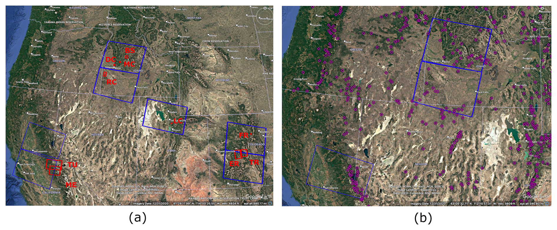
Figure 1 Imagery © Google Earth Pro, Map data © 2025 Google, (a) of Sentinel-1 frames (blue rectangles) and LIDAR data (red rectangles). (b) of Sentinel-1 frames (blue rectangles) with 6 hours revisit time and SNOTEL stations (purple diamonds).

The NASA SnowEx2020 and 2021 Time Series represents a continuation of the multi-year initiative to advance snow water equivalent (SWE) measurement and estimation. Data acquisition during winter 2020 and 2021 included multiple sensors (e.g., radar and LIDAR) and in situ collections. As part of this effort, the SnowEx campaign collaborated with the Sentinel-1 team to obtain six-day revisit observations over selected sites throughout the winter season. The blue frames in Fig. 1a show the geographic locations of Sentinel-1 data that cover the available LIDAR data in 2020 or 2021. The blue frames in Fig. 1b show the geographic locations of all Sentinel-1 data with 6 d revisit time during the winter of 2020 and 2021 that cover more than 5 SNOTEL stations. Our analysis indicated that snow water equivalent (SWE) retrieval using Sentinel-1 data performs better with 6:00 am acquisitions compared to 6:00 pm data. Consequently, the majority of our study focuses on results derived from descending Sentinel-1 acquisitions collected at 6:00 am local time; however, a performance comparison between ascending (6:00 pm) and descending (6:00 am) data over two LIDAR sites is provided in Sect. 4.1.2.

3.2 LIDAR

Airborne LIDAR provides high-resolution snow depth maps and serves as a reliable source of validation data, offering a particularly strong constraint for InSAR-based retrieval of SWE. For this study, we surveyed all publicly available LIDAR datasets and selected those collected during the snow accumulation season. The “SnowEx20-21 QSI LIDAR DEM 0.5m” dataset, part of the SnowEx 2020 and 2021 campaigns, includes digital elevation models, snow depth, and vegetation height at 5 m spatial resolution (Adebisi et al., 2022). To enable direct comparison with Sentinel-1-derived SWE, the LIDAR data were resampled to 80 m resolution. These data were acquired over sites in Colorado, Idaho, and Utah during February 2020, March 2021, and September 2021. In addition, the Airborne Snow Observatory (ASO) program has been operating since 2013, providing over a decade of high-resolution snow observations across the western United States. ASO products combine LIDAR, imaging spectrometry, and physically based modeling to generate snow depth and snow water equivalent estimates (Deems et al., 2013; Painter et al., 2016). The snow depth measurements have an accuracy of approximately 3 cm with a spatial resolution of 3 m. While early ASO campaigns focused on the melt season, current operations span a broader period from January through July, reflecting the importance of both accumulation and melt processes for water resource management. For this study, we used all publicly available ASO datasets collected between January and March. All ASO datasets included in Table 1 were processed and provided by the ASO program.

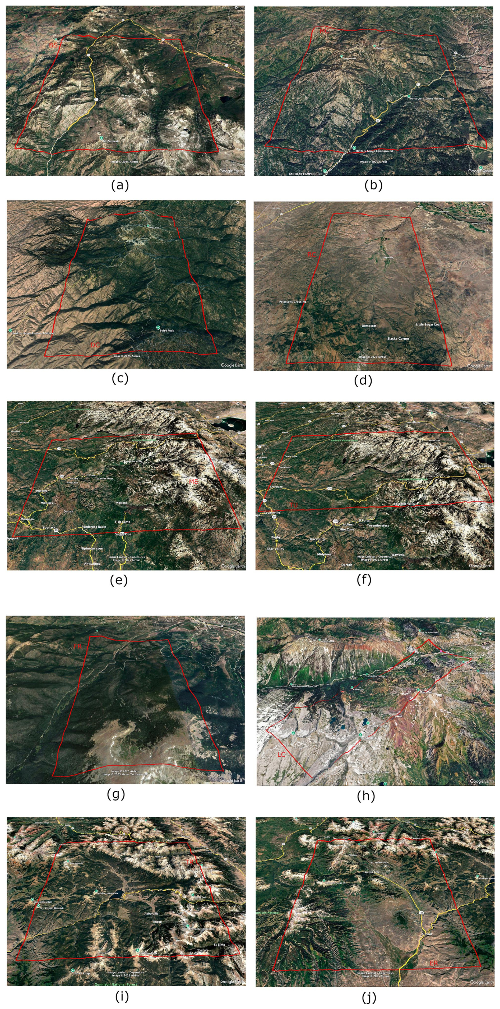
Figure 2 Imagery © Google Earth Pro, Map data © 2025 Google, of LIDAR scenes (a) Banner Summit, ID (b) Mores Creek, ID (c) Dry Creek, ID (d) Reynolds Creek, ID (e) Merced, CA (f) Tuolumne, CA (g) Fraser, CO (h) Little Cottonwood Canyon, UT (i) East River, CO (j) Taylor River, CO.

As mentioned LIDAR snow depth data is a very valuable dataset for validating our retrieved SWE. The red boxes in Fig. 1a show the location of LIDAR data acquisition during the dry snow regions.

Figure 2a–j show the zoomed Google Earth View of LIDAR scenes, Banner Summit, ID (BS), Mores Creek, ID (MC), Dry Creek, ID (DC), Reynolds Creek, ID (RC), Merced, CA (ME), Tuolumne, CA (TU), Fraser, CO (FR), Little Cottonwood Canyon, UT (LC), East River, CO (ER), Taylor River, CO (TR), respectively.

Table 1 Information about LIDAR scenes used in this study. First column shows the site ID. The second column shows the company collecting the data. The third column shows the LIDAR acquisition date. Columns four and five show the revisit time and path/frame of Sentinel-1 time series covering the LIDAR scene, respectively. Last column show the correlation between LIDAR snow depth and retrieved SWE using Sentinel-1 data.

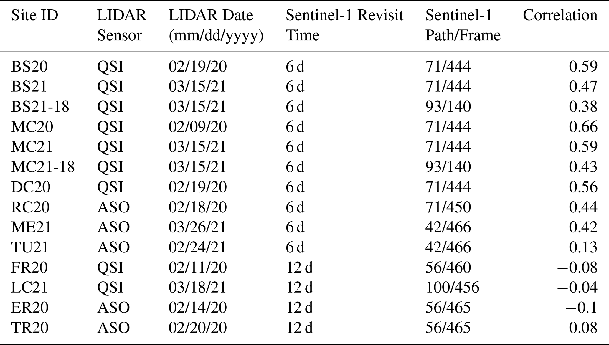
Table 1 summarizes all LIDAR scenes used in this study, consisting of data collected between January and March of 2020 and 2021. The first column lists the LIDAR site ID, followed by the data provider in the second column. The third column reports the date of LIDAR acquisition, while the fourth and fifth columns provide the revisit time and the corresponding Sentinel-1 path/frame information for the time series covering each LIDAR scene. The LIDAR data are subsequently used in Sects. 4.1 and 5.1 to evaluate the performance of SWE retrievals derived from Sentinel-1 observations.

3.3 SNOTEL

The SNOwpack TELemetry (SNOTEL) network consists of stations located in remote, high-elevation mountain regions across the western United States. These stations automatically record a range of snowpack and meteorological variables. For this study, hourly SNOTEL observations were accessed through the United States Department of Agriculture (USDA) website (USDA, 2025). Because we used descending Sentinel-1 acquisitions, collected at approximately 6 am local time, we extracted SNOTEL measurements of SWE, snow depth, and near-surface air temperature corresponding to that time. The locations of the SNOTEL stations are shown as purple diamonds in Fig. 1b. Notably, during winter 2021, only three Sentinel-1 frames with 6 d repeat cycles covered more than five SNOTEL sites. These in situ measurements were employed for (a) establishing InSAR reference points (Sect. 2.1), (b) evaluating the performance of SWE retrievals (Sect. 4.2), and (c) analyzing the influence of environmental parameters on SWE retrieval accuracy (Sect. 5.2).

4 Performance of SWE Retrieval Using Sentinel-1 interferometric Phase

Unlike (Oveisgharan et al., 2024), which focused on demonstrating the feasibility of SWE retrieval using Sentinel-1 interferometry over a limited number of sites, this section evaluates retrieval performance across a broader range of snow conditions and land-cover types to identify the key factors controlling retrieval accuracy. In this section, we assess the performance of SWE retrievals derived from Sentinel-1 data. Section 4.1 presents a comparison with LIDAR snow depth measurements, while Sect. 4.2 evaluates retrieval performance against SNOTEL ΔSWE observations.

4.1 Comparing the Retrieved SWE with LIDAR data

As summarized in Table 1 and illustrated in Figs. 1 and 2, a total of 10 LIDAR scenes with snow depth measurements were available between January and March of 2020 and 2021. Among these, the Banner Summit (BS) and Mores Creek (MC) sites contain data for both years. For each LIDAR scene, we used the corresponding Sentinel-1 time series (path and frame information provided in Table 1, column 5) to retrieve ΔSWE following the approach described in Sect. 2. Following Oveisgharan et al. (2024), time-series-derived ΔSWE was then used to estimate total SWE at the date closest to the LIDAR acquisition by

$$\begin{array}{}\text{(3)}& \mathrm{SWE}\left(t_{i+\mathrm{1}}\right)=\sum _{t_j=t_{\mathrm{1}}}^{t_{\mathrm{i}}}\mathrm{\Delta }\mathrm{SWE}(t_j,t_{j+\mathrm{1}})\end{array}$$

where t₁ is the first Sentinel-1 data collected after December first of the corresponding winter and t_i+1 is the closest Sentinel-1 date to LIDAR acquisition date. For simplicity, we assume the SWE at time t₁ is equal to zero. The assumption of zero SWE at t₁ may introduce a bias in the reconstructed total SWE in regions where early-season accumulation is present. However, this assumption primarily affects the absolute magnitude of SWE rather than its spatial variability. For example, based on in situ measurements distributed across the Sentinel-1 frame (p71, f444), the spatial standard deviation of SWE is approximately 5 cm at the beginning of December and increases to about 23 cm by the end of March. This indicates that early-season SWE exhibits relatively low spatial variability compared to peak winter conditions. Given that the LIDAR scenes cover a much smaller spatial extent (∼ 16 km × 15 km) within the larger Sentinel-1 frame (∼240 km × 240 km), the spatial variability of SWE at the beginning of December is expected to be even smaller at the LIDAR scale. Therefore, neglecting the initial SWE mainly introduces an approximately constant offset in the reconstructed SWE and is not expected to significantly affect the spatial correlation with LIDAR snow depth. However, the reconstructed SWE values may be systematically biased low in absolute terms.

It is important to note that the Sentinel-1-based retrieval estimates SWE, whereas the LIDAR observations provide snow depth. As a result, the comparison between retrieved SWE and LIDAR snow depth is not strictly one-to-one. Although LIDAR snow depth could be converted to SWE using an assumed snow density, such a conversion would introduce additional uncertainty associated with density estimation. The correlation metric used here implicitly assumes a constant snow density across each scene. Despite this simplifying assumption, the results show reasonable agreement as seen in Sect. 4.1. This limitation should be considered when interpreting the comparisons. The effective density implied by the comparison between retrieved SWE and LIDAR snow depth is further evaluated in Sect. 4.1.4.

Another important consideration is the difference in spatial resolution and sampling geometry among the datasets. The Sentinel-1 products used in this study have an effective spatial resolution of approximately 80 m after multilooking, whereas the LIDAR data are available at 0.5 and 3 m resolution, and SNOTEL measurements represent point-scale observations. To improve consistency, the LIDAR data were spatially averaged to 80 m resolution prior to comparison. Nonetheless, residual differences in spatial representativeness remain. In addition, the observation geometries differ: Sentinel-1 is a side-looking system with look angles of approximately 29–46°, whereas LIDAR measures snow depth in the nadir direction. Consequently, the sampled snowpack, vegetation, and ground characteristics are not identical between the datasets. Spatial variability in snow properties, vegetation structure, and terrain within the 80 m comparison scale may further contribute to discrepancies. Terrain slope in complex topography can affect both LIDAR measurements and InSAR-derived SWE. For LIDAR, steep slopes may introduce sampling biases and noise in snow depth estimation, while for InSAR, slope influences the local incidence angle and the effective radar propagation path through the snowpack, thereby affecting the interferometric phase and the retrieved SWE. In addition, steep terrain can introduce radar-specific effects such as layover and shadow, which further degrade signal quality and coherence and can impact retrieval accuracy. Because the radar footprint is significantly larger than that of LIDAR, these effects can be more pronounced in the InSAR observations. A more rigorous treatment of slope effects, including explicit modeling of radar–snow interaction geometry, is beyond the scope of this study. However, the impact of slope is partially addressed by including terrain slope as one of the parameters in the retrieval performance analysis (Sect. 5.1). Its influence is also evident in the comparison between ascending and descending acquisitions discussed in Sect. 4.1.2. These factors should be considered when interpreting validation results, as some observed differences or dependencies may arise from mismatches in measurement geometry and resolution rather than from retrieval performance alone.

To evaluate performance, the analysis was divided into two groups: LIDAR scenes covered by Sentinel-1 data with 6 d revisit intervals and those with 12 d revisit intervals. As shown in Table 1, eight scenes fall into the 6 d repeat group, while four scenes correspond to 12 d repeats.

4.1.1 Using 6 d Repeat Sentinel-1 Data

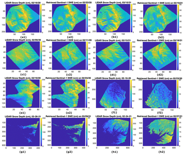
Figure 3a1–h1 present LIDAR-derived snow depth for Banner Summit (18 February 2020 and 15 March 2021), Mores Creek (9 February 2020 and 19 March 2021), Dry Creek (19 February 2020), Reynolds Creek (23 February 2020), Merced (26 March 2021), and Tuolumne (27 February 2021). The corresponding retrieved total SWE, derived from Sentinel-1 6 d time series using Eq. (3), is shown in Fig. 3a2–h2. We refer to each LIDAR scene by site abbreviation and year (e.g., BS20 = Banner Summit 2020, MC21 = Mores Creek 2021). For each case, the Sentinel-1 acquisition date closest to the LIDAR survey date (t_i+1 in Eq. 3) is indicated in the figure titles. Overall, the retrieved SWE fields show strong visual agreement with the LIDAR snow depth maps. The Pearson correlation coefficients between LIDAR snow depth and Sentinel-1-derived SWE, reported in the last column of Table 1, range from 0.42 to 0.66 across sites, with the exception of Tuolumne (TU).

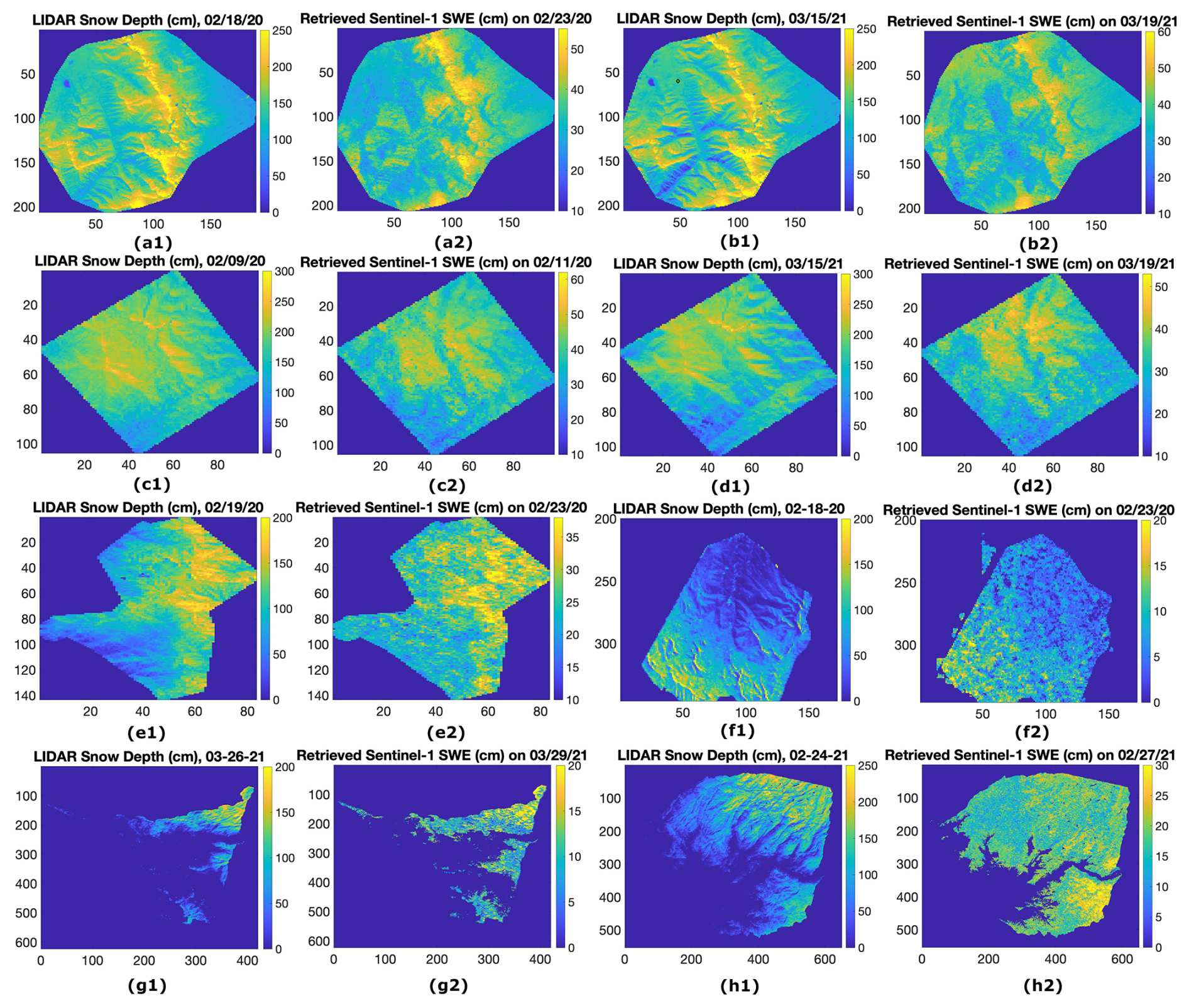
Figure 3 LIDAR total snow depth (a1–h1) for Banner Summit on 18 February 2020, Banner Summit on 15 March 2021, Mores Creek on 9 February 2020, Mores Creek on 19 March 2021, Dry Creek on 19 February 2020, Reynolds Creek on 23 February 2020, Merced on 26 March 2021, and Tuolumne on 27 February 2021, respectively. Images (a2–h2) show the total retrieved SWE using 6 d repeat Sentinel-1 time series data from 1 December to closest date to LIDAR date acquisition, respectively.

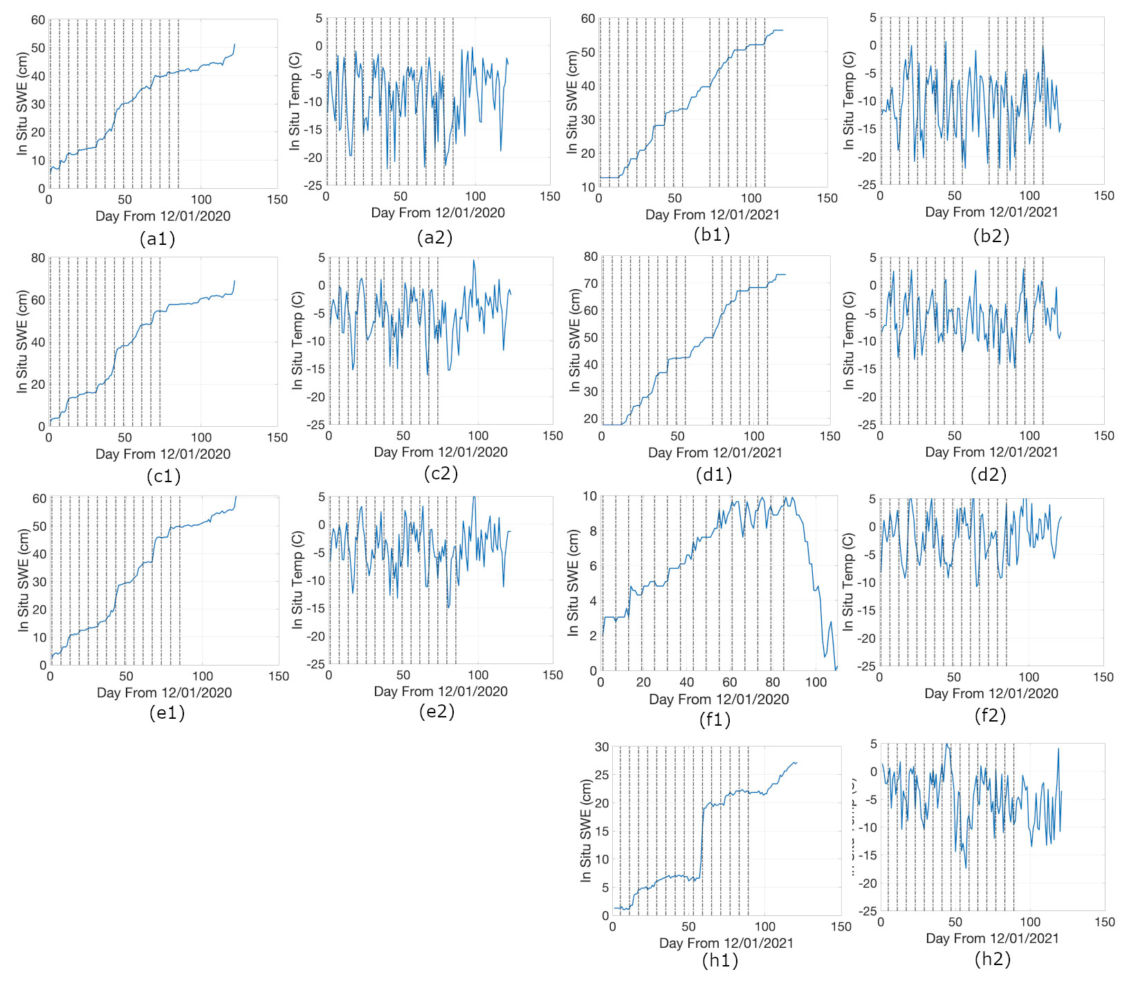
Figure 4 SWE (a1–h1) and Temperature (a2–h2) for SNOTEL stations inside BS in 2020, BS in 2021, MC in 2020, MC in 2021, DC in 2020, RC in 2020, ME in 2021, and TU in 2021, respectively. The dashed vertical lines show the start date of Sentinel-1 observations.

Within the LIDAR frames shown in Fig. 3a1–h1, all scenes except Merced (Fig. 3g1) contain at least one SNOTEL site. Figure 4a1–h1 present the total SWE time series from these SNOTEL stations, beginning on December 1 of the corresponding winter. Figure 4a2–h2 show the corresponding near-surface air temperature time series. The dashed vertical lines mark the start dates of each 6 d Sentinel-1 acquisition cycle. Notably, a data gap occurred on 5 February 2021, resulting in a missing six-day repeat acquisition.

The correlation between retrieved SWE and LIDAR snow depth varies across sites, with lower values observed for Reynolds Creek (RC) and Merced (ME) compared to Banner Summit (BS), Mores Creek (MC), and Dry Creek (DC). The correlation is particularly weak at Tuolumne (TU). As shown in Fig. 4f1–f2, total SWE and SWE changes between Sentinel-1 acquisitions were minimal for RC20, while temperatures exceeded 0 °C on 25 d during the season before LIDAR acquisition date. The presence of wet snow and limited SWE variability degrades retrieval performance (Oveisgharan et al., 2024), explaining the weaker correlation at RC20. Although Merced lacks a co-located SNOTEL site, it is geographically close to TU, and therefore SNOTEL data from the TU frame were used as a proxy. Between 1 December and the corresponding LIDAR acquisition dates, the number of days with above-freezing temperatures at SNOTEL stations was 0, 1, 4, 7, 10, 25, and 16 for BS20, BS21, MC20, MC21, DC20, RC20, and TU21, respectively. These higher temperatures and more frequent melt events in RC, ME, and TU contributed to the reduced correlations between Sentinel-1-derived SWE and LIDAR snow depth. A large snowstorm was also observed at TU, with an SWE increase of 8.89 cm between 22 and 28 January 2021 (acquisition 9). Although the overall correlation between retrieved SWE and LIDAR snow depth at TU21 was low (0.13), the correlation between LIDAR snow depth and retrieved ΔSWE during this storm (acquisition 9) reached 0.6. This suggests that melt events during other periods were responsible for degrading retrieval performance at TU21.

4.1.2 Using 6 am and 6pm Sentinel-1 Data

In this section, we compare SWE retrieval performance using Sentinel-1 acquisitions from 6 am (descending) and 6 pm (ascending) passes. Figure 5a and c show the retrieved SWE using 6 am and 6 pm time series, respectively, up to the date closest to the LIDAR acquisition on 15 March 2021. The corresponding correlations with LIDAR snow depth (Table 1, rows 3 and 4) are 0.47 and 0.38, respectively. The 6 am retrieval shows a stronger spatial agreement with LIDAR, consistent with the higher correlation.

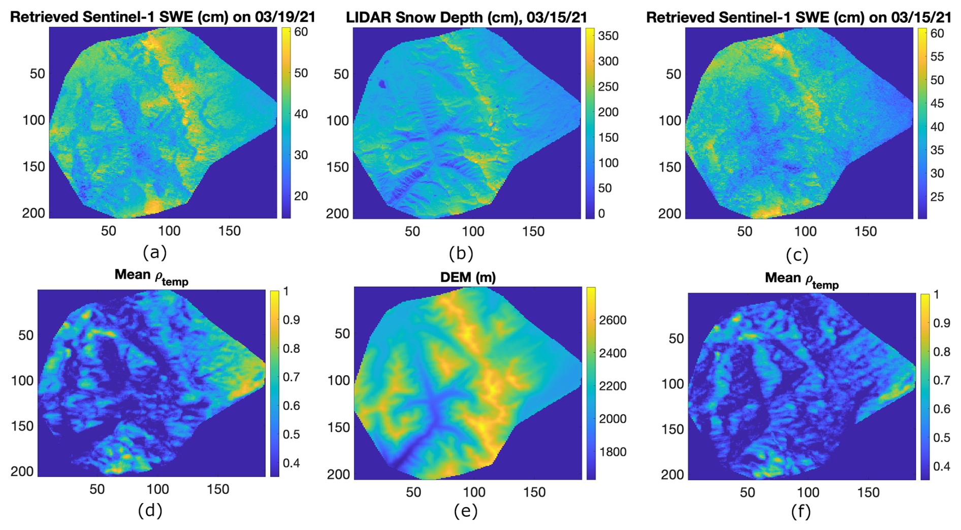
Figure 5 Total retrieved SWE using 6 d repeat Sentinel-1 time series data for (a) 6 am and (c) 6 pm acquisitions, accumulated from December 1 to the date closest to the LIDAR acquisition over Banner Summit. (b) LIDAR-derived total snow depth on 15 March 2021. Mean Sentinel-1 temporal coherence for (d) 6 am and (f) 6 pm acquisitions. (e) Digital elevation model (DEM) of the Banner Summit study area.

This improvement is likely due to more favorable snow conditions in the early morning. Lower temperatures reduce melt and maintain drier snow, which improves phase stability and retrieval accuracy. The mean temporal coherence for the 6 am and 6 pm datasets (Fig. 5d and e) is 0.51 and 0.46, respectively, further supporting this observation.

However, spatial variations in coherence reveal a more nuanced behavior. In certain areas within the scene, temporal coherence is lower in the 6 am data but higher in the 6 pm data. In these regions, the retrieved SWE from the 6 pm acquisitions shows better agreement with LIDAR. As shown in Fig. 5f, these regions correspond to slopes that face away from the satellite in the descending (6 am) geometry and toward the satellite in the ascending (6 pm) geometry. When slopes face away from the radar, backscatter is reduced, leading to lower signal-to-noise ratio (SNR), reduced coherence, and degraded retrieval performance.

These results highlight a trade-off between environmental conditions and imaging geometry. While morning acquisitions generally provide better conditions for SWE retrieval due to colder and drier snow, afternoon acquisitions can improve performance in areas with unfavorable viewing geometry in the morning.

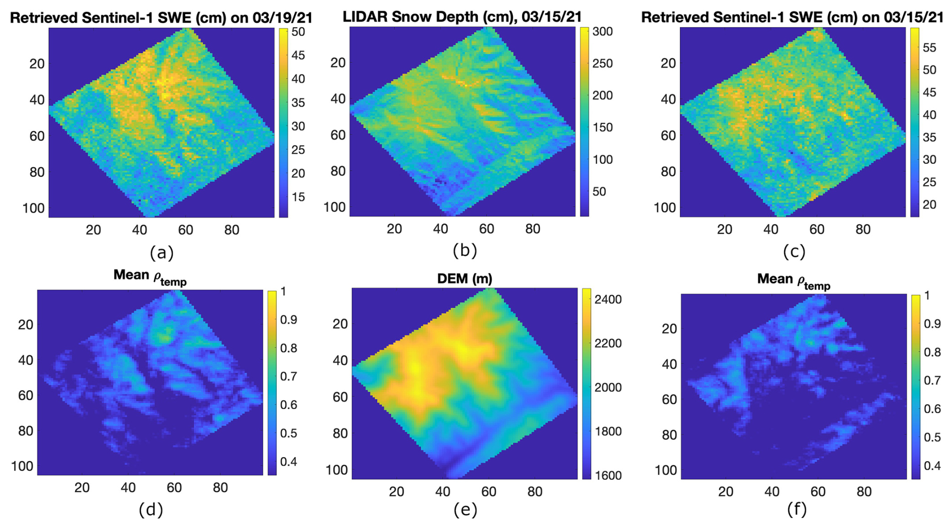
Figure 6 Total retrieved SWE using 6 d repeat Sentinel-1 time series data for (a) 6 am and (c) 6 pm acquisitions, accumulated from December 1 to the date closest to the LIDAR acquisition over Mores Creek. (b) LIDAR-derived total snow depth on 15 March 2021. Mean Sentinel-1 temporal coherence for (d) 6 am and (f) 6 pm acquisitions. (e) Digital elevation model (DEM) of the Banner Summit study area.

Figure 6 presents the same comparison for the Mores Creek site on 15 March 2021. The correlation decreases from 0.59 (6 am) to 0.43 (6 pm), and the mean temporal coherence decreases from 0.42 to 0.37. Similar geometric effects are observed, with improved performance in areas facing the satellite during the afternoon pass. These findings suggest that combining ascending and descending acquisitions may improve SWE retrieval by compensating for spatial variations in coherence related to viewing geometry. Such fusion strategies should be considered in future work.

4.1.3 Using 12 d Repeat Sentinel-1 Data

Figure 7a1–d1 present LIDAR-derived snow depth for Fraser (FR20, 11 February 2020), Little Cottonwood Canyon (LC21, 18 March 2021), East River (ER20, 14 February 2020), and Taylor River (TR20, 20 February 2020). The corresponding retrieved SWE, derived using Eq. (3) and Sentinel-1 12 d time series, is shown in Fig. 7a2–d2. For each case, the Sentinel-1 acquisition date closest to the LIDAR survey (t_i+1 in Eq. 3) is indicated in the figure titles. Unlike the 6 d repeat results, these scenes show little resemblance between LIDAR snow depth and Sentinel-1-derived SWE. The Pearson correlation coefficients range from −0.1 to 0.08, confirming that a 12 d revisit interval is too coarse for SWE retrieval using C-band Sentinel-1 data.

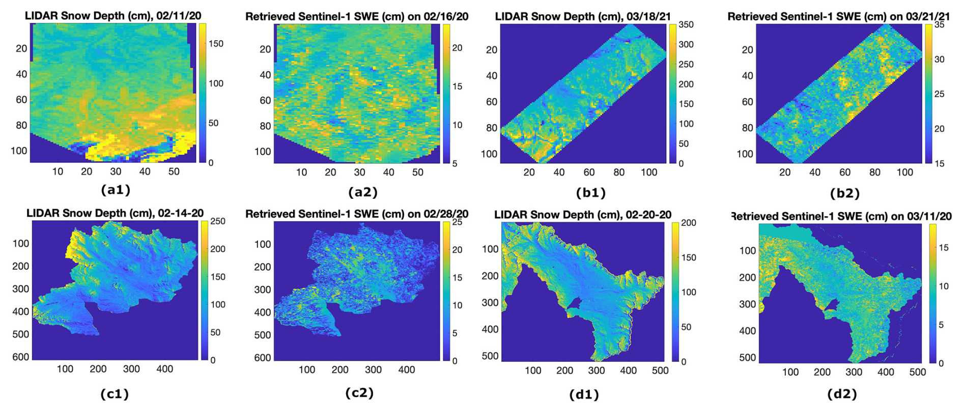
Figure 7 LIDAR total snow depth (a1–d1) for Fraser on 11 February 2020, Little Cottonwood Canyon on 21 March 2021, East River on 14 February 2020, and Taylor River on 11 March 2020. Images (a2–d2) show the total retrieved SWE using 12 d repeat Sentinel-1 time series data from 1 December to closest date to LIDAR date acquisition, respectively.

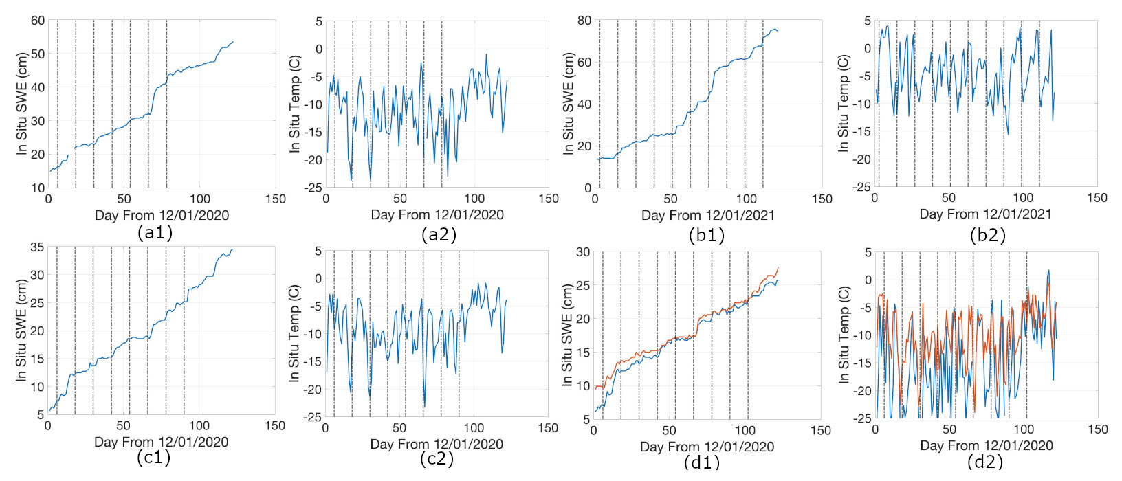
Figure 8 SWE (a1–d1) and Temperature (a2–h2) for SNOTEL stations inside FR in 2020, LC in 2021, ER in 2020, and TR in 2020, respectively. The dashed vertical lines show the start date of Sentinel-1 observations. In panels (d1) and (d2), the red and blue curves represent two different SNOTEL stations within the TR20, whereas only a single station (blue curve) is available in the other panels.

Figure 8a1–d1 display the SNOTEL SWE time series within the LIDAR frames of Fig. 7a1–d1, beginning December 1 of the corresponding winter. The associated near-surface temperature time series are shown in Fig. 8a2–d2. Dashed vertical lines mark the start dates of each 12 d Sentinel-1 acquisition cycle. In panels (d1) and (d2), the red and blue curves represent two different SNOTEL stations within the scene, whereas only a single station (blue curve) is available in the other panels. The SNOTEL SWE and temperature records are later used in Sect. 5.1.1 to investigate the environmental factors influencing temporal coherence. The results (not shown here) indicate that temporal coherence degrades significantly at the 12 d revisit interval, rendering the data unreliable for SWE retrieval. This degradation arises from a combination of factors rather than a single dominant limitation. First, the longer temporal baseline increases decorrelation due to snowpack evolution, wind redistribution, and melt–freeze processes, which reduces the reliability of the interferometric phase. As discussed in Sect. 4.1.5, low temporal coherence leads to a substantial increase in SWE retrieval uncertainty and degrades the performance of phase unwrapping algorithms. Second, the magnitude of SWE change between acquisitions is significantly larger for 12 d intervals compared to 6 d intervals (e.g., Fig. 8 versus Fig. 4). For Sentinel-1, the SWE ambiguity corresponding to a 2π phase cycle ranges from approximately 1.5 to 3.5 cm depending on incidence angle. In many cases, the accumulated ΔSWE over 12 d exceeds this ambiguity threshold, making phase unwrapping more challenging and increasing the likelihood of phase errors. While such ambiguities can sometimes be resolved using high-coherence reference areas combined with in situ constraints, the simultaneous presence of low coherence limits the effectiveness of these approaches. Finally, longer revisit intervals increase the probability of transient melt events and wet-snow conditions occurring between acquisitions, which violate the dry-snow assumption required for the interferometric SWE retrieval. In addition, the reduced number of acquisitions in a 12 d time series increases the relative weight of each interferogram in reconstructing total SWE, making the retrieval more sensitive to individual errors. Overall, the combination of increased temporal decorrelation, larger SWE changes relative to phase ambiguity, reduced phase unwrapping reliability, and a higher likelihood of wet-snow conditions makes SWE retrieval from 12 d Sentinel-1 data significantly more challenging. It is worth noting that upcoming missions such as NISAR, despite having a similar nominal 12 d repeat cycle, operate at longer wavelengths (L- and S-band), which are expected to maintain higher temporal coherence and provide larger SWE ambiguity thresholds (approximately 6–14 cm). These characteristics are anticipated to mitigate some of the limitations observed for C-band Sentinel-1 data.

4.1.4 Evaluating the Retrieved Snow Density

As discussed earlier, the strong correlation observed between LIDAR snow depth and retrieved SWE provides an important indication of retrieval performance. In that comparison, an implicit assumption is that a constant snow density (e.g., using the ratio of mean SWE to mean snow depth) can reasonably relate the two quantities. Here, we instead compute the ratio of retrieved SWE to LIDAR snow depth at each pixel as an estimate of the effective snow density. In this case, the comparison becomes internally consistent (i.e., the relationship between SWE and snow depth is directly enforced), and the objective is to assess whether the resulting density values fall within a physically realistic range. As noted earlier, LIDAR provides measurements of snow depth, whereas Sentinel-1-based retrieval yields SWE. An effective snow density can therefore be estimated as the ratio of retrieved SWE to LIDAR snow depth.

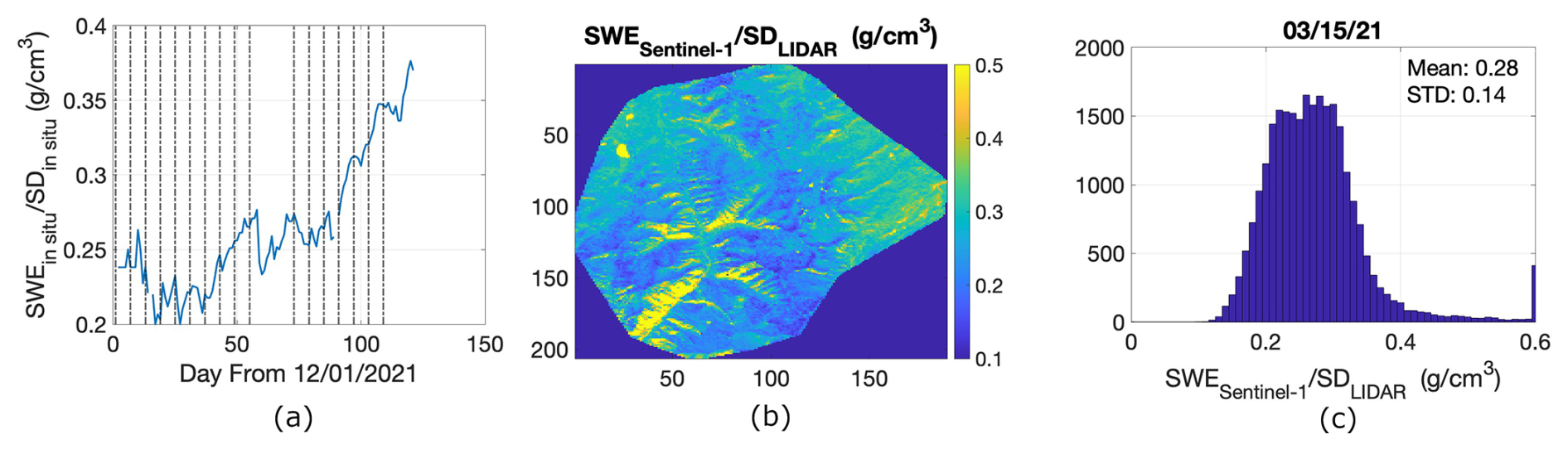
Figure 9 Banner Summit (2021): (a) in situ snow density time series; (b) ratio of Sentinel-1-retrieved SWE to LIDAR snow depth; (c) histogram of the ratio of Sentinel-1-retrieved SWE to LIDAR snow depth.

As an example, we evaluate the effective snow density over Banner Summit in 2021, as shown in Fig. 9. The results in Fig. 9b and c indicate that the estimated densities fall within a reasonable range for terrestrial snow and are broadly consistent with the in situ snow density measurements during the snow snow season shown in Fig. 9a. While the in situ measurements in Fig. 9a show that snow density generally increases throughout the winter season as the snowpack compacts and metamorphoses, this temporal evolution should not be interpreted as a spatial relationship. At a given time, snow density is controlled by several factors, including snow history, wind redistribution, temperature, and metamorphism, and therefore does not necessarily increase with local snow depth. Consequently, it is difficult to assess the physical realism of the retrieved density map solely based on its spatial distribution. Nevertheless, the estimated snow densities provide two additional indications of the physical consistency of the retrieval. First, the distribution of the retrieved snow density, including its mean and standard deviation, is consistent with the range and variability observed in the in situ density measurements shown in Fig. 9a. Second, the estimated density map exhibits a smooth and spatially coherent pattern rather than noisy pixel-to-pixel variations, despite being derived from two independent datasets (Sentinel-1 SWE and LIDAR snow depth). Comparison with the LIDAR snow depth map in Fig. 5b further suggests that regions of deeper snow tend to correspond to slightly lower estimated densities. Although this pattern appears physically plausible for this site, a more rigorous assessment would require independent spatial measurements of snow density, which were not available for this study. Some high-density outliers are observed in Fig. 9b (yellow regions) and also in the histogram in Fig. 9c. Comparison with the mean temporal coherence shown in Fig. 5d indicates that many of these areas correspond to regions of low temporal coherence, where the uncertainty in SWE retrieval is higher. This suggests that errors in low-coherence regions can lead to unrealistically high density estimates. Overall, the combination of strong correlation between retrieved SWE and LIDAR snow depth, together with physically reasonable estimates of snow density, supports the reliability of the SWE retrieval.

4.1.5 Evaluating the Uncertainty of Retrieved SWE for LIDAR

In this section, we assess the uncertainty in SWE retrieval derived from Sentinel-1 data. The analysis focuses on errors affecting the interferometric phase measurement and the resulting SWE estimates. Uncertainties associated with the phase-to-SWE conversion model are not considered here. In particular, factors such as snow wetness and temperature, which violate the dry-snow assumption underlying the retrieval model, are not evaluated, as they require a different physical framework. As noted earlier, the primary sources of error in Sentinel-1 phase measurements are temporal decorrelation and tropospheric delay. The total SWE shown in Fig. 3 is obtained by cumulatively summing SWE changes derived from the InSAR time series.

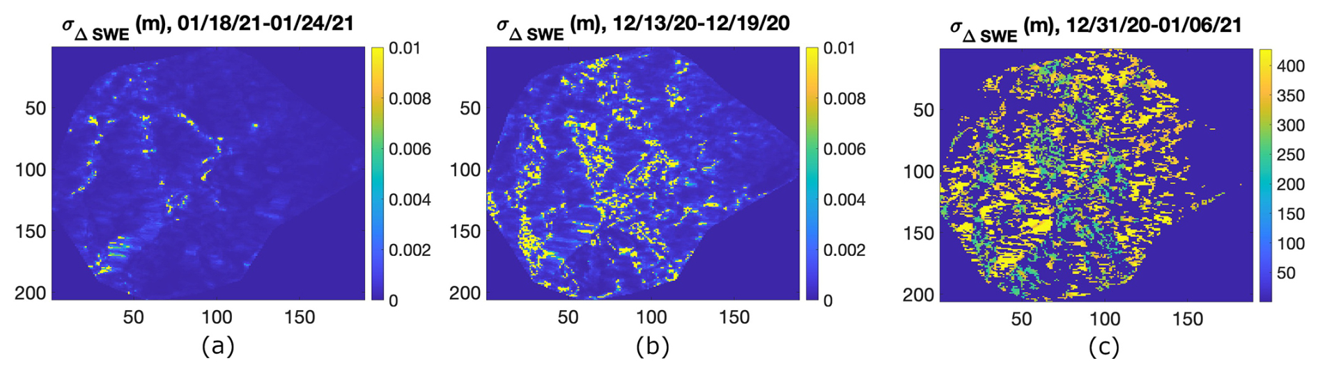
Figure 10 The estimated SWE change error (m) due to temporal coherence over Banner Summit between (a) 18 and 24 January 2021 (b) 13 and 19 December 2020 (c) 31 December 2020 and 6 January 2021.

Figure 10a–c illustrate the estimated SWE change error between two acquisition dates (indicated in the titles) due to temporal coherence over Banner Summit in 2021. The total error is computed as the root-sum-square of individual error contributions, following Eq. (2). As temporal coherence decreases from Fig. 10a to c, the uncertainty in SWE correspondingly increases. For relatively high coherence, the error is on the order of a few millimeters. In contrast, for very low coherence, the error increases dramatically, reaching values on the order of tens of meters, rendering the estimates unreliable. This behavior highlights that interferometric measurements with coherence below approximately 0.3 are not suitable for SWE retrieval. While the full time series is used here to reconstruct total SWE for comparison with LIDAR snow depth, future SWE change time series products should incorporate a quality flag based on coherence thresholds. Another important source of uncertainty arises from tropospheric delay. As described earlier, ERA5 atmospheric reanalysis product were used to correct for tropospheric effects. The residual tropospheric error is expected to be on the order of a few centimeters over the full Sentinel-1 scene (approximately 240 km × 240 km). Due to the spatial power spectrum of atmospheric variability (Agnew, 1992), the magnitude of this error decreases at smaller spatial scales and is expected to be less than 1 cm (0.3–0.5 cm) over the LIDAR scene (∼ 16 km × 15 km). However, the turbulence in the atmosphere can still introduce few cm of errors.

4.2 Comparing the Retrieved SWE Using Sentinel-1 with SNOTEL SWE

As described in Sect. 3.1, Sentinel-1 data were acquired every 6 d over three frames containing more than five SNOTEL sites (Fig. 1b) during 2020 and 2021, coordinated between the SnowEx campaign and the Sentinel-1 team. For this analysis, we used 6 d repeat Sentinel-1 time series from 1 December 2020 to 30 March 2021.

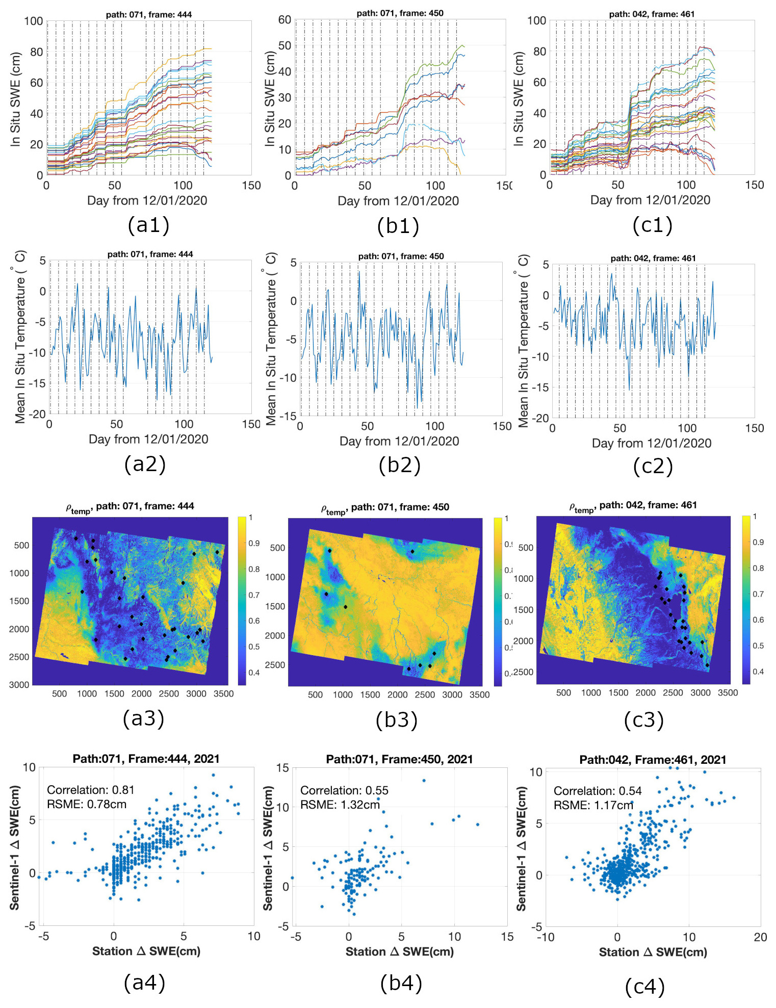
Figure 11 (a1) SNOTEL SWE measurements (cm) for all stations in Sentinel-1 (p71, f444) starting December first to end of March. Different colors show the measurements for different SNOTEL stations. (a2) Mean of all SNOTEL temperature measurements (°C) in Sentinel-1 (p71, f444) starting December first to end of March. (a3) Mean of Sentinel-1 temporal coherence for (p71, f444) starting December first to end of March. (a4) Retrieved ΔSWE vs SNOTEL ΔSWE for (p71, f444) every 6 d starting December first to end of March. Panels (b1)–(b4) and (c1)–(c4) are the same as Panels (a1)–(a4), but use Sentinel-1 data from (p71, f450) and (p42, f461), respectively.

The left, middle, and right columns of Fig. 11 correspond to frames (p71, f444), (p71, f450), and (p42, f461), respectively. Figure 11a1–c1 show SNOTEL SWE time series from 1 December 2020 to 31 March 2021 at 6:00 am for all stations within each frame, with different colors indicating individual SNOTEL sites. SWE increases relatively uniformly in (p71, f444), whereas sharp increases are observed in (p71, f450) and (p42, f461). Snowpack is also generally shallower in (p71, f450).

Figure 11a2–c2 present the average near-surface temperature across SNOTEL stations in each frame. Among them, (p42, f461) is consistently warmer than (p71, f444) and (p71, f450). Figure 11a3–c3 display the average Sentinel-1 temporal coherence time series, with black squares marking SNOTEL locations. Low-coherence regions align with snow-covered areas. Frame (p71, f450) exhibits higher coherence due to its shallower snowpack, while (p42, f461) shows lower coherence compared to (p71, f444).

Figure 11a4–c4 compare retrieved ΔSWE from Sentinel-1 time series with ΔSWE from SNOTEL stations over the study period. It is important to note the differences in spatial resolution and sampling geometry between the datasets. The Sentinel-1 products used in this study have an effective spatial resolution of approximately 80 m after multilooking, whereas SNOTEL measurements represent point-scale observations. To reduce the impact of spatial heterogeneity and improve comparability, we further averaged Sentinel-1-derived SWE change over a 10 × 10 pixel window centered on each SNOTEL site, corresponding to an effective spatial resolution of approximately 800 m. This spatial averaging helps mitigate mismatches between point measurements and distributed estimates. The correlation coefficients are 0.81, 0.55, and 0.54 for frames (p71, f444), (p71, f450), and (p42, f461), respectively. The corresponding RMSE values are 0.78, 1.32, and 1.17 cm. The reduced performance in (p71, f450) and (p42, f461) is attributed to limited SWE change in the former and warmer temperatures in the latter.

4.2.1 Evaluating the Uncertainty of Retrieved SWE for SNOTEL Data

In this section, we assess the uncertainty in SWE retrieval derived from Sentinel-1 data at SNOTEL locations. Similar to the analysis in Sect. 4.1.5, Eq. (2) is used to estimate SWE change error due to temporal coherence. The analysis focuses on uncertainties associated with interferometric phase measurements and their propagation into SWE estimates, and does not include uncertainties related to the phase-to-SWE conversion model.

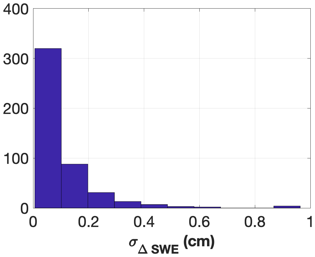
Figure 12 Histogram of estimated SWE change error (cm) due to temporal coherence for all SNOTEL stations within frame (p81, f444) from December 2020 to March 2021.

Figure 12 illustrates the histogram of estimated SWE change error due to temporal coherence for all SNOTEL stations within frame (p81, f444) from December 2020 to March 2021. The error magnitude is comparable to that shown in Fig. 10a, corresponding to coherence mostly greater than 0.1. This is primarily because, for each in situ station, coherence is averaged over a 10 × 10 window. Combined with the multilooking applied to generate the 80 m resolution data (20 × 4 looks), this averaging reduces noise and brings the measured coherence closer to the true coherence. As a result, very low coherence values (e.g., below 0.1) are rarely observed at SNOTEL locations. Consequently, SWE change estimates at in situ stations exhibit lower uncertainty compared to pixel-wise estimates evaluated against LIDAR data. For future SWE change time series products, the inclusion of a quality flag based on coherence thresholds is recommended. Another important source of uncertainty is tropospheric delay. After correction using ERA5 atmospheric reanalysis data, the residual tropospheric error is expected to be on the order of a few centimeters over the full Sentinel-1 scene (approximately 240 km × 240 km). Since SNOTEL stations are distributed across the entire frame, stations located farther from the reference point may experience larger residual errors. Based on the spatial power spectrum of atmospheric variability (Agnew, 1992), the residual tropospheric error is expected to range from near zero up to a few centimeters (approximately 0.7–1.5 cm), depending on the distance from the reference point. In addition, small-scale atmospheric turbulence may introduce further variability on the order of a few centimeters at individual stations. Therefore, for SNOTEL-based SWE change estimates, tropospheric delay is likely the dominant source of uncertainty.

5 Impact of Different Parameters on SWE Retrieval

While previous work (Oveisgharan et al., 2024) established the capability of InSAR to retrieve SWE, it did not systematically assess the environmental and geophysical controls on retrieval performance. Here, we extend that work by analyzing how factors such as temporal coherence, temperature, vegetation, and terrain influence retrieval accuracy across multiple sites. As demonstrated in Sect. 4.1 and 4.2, the correlation between Sentinel-1-retrieved SWE or ΔSWE and validation datasets (LIDAR snow depth or SNOTEL ΔSWE) varies across sites. In this section, we investigate the key factors influencing these correlations.

5.1 Impact of Different Parameters on Retrieved SWE Using LIDAR Data

In this section, we assess how various parameters influence the performance of SWE retrieval from Sentinel-1 by comparing retrieved SWE against LIDAR snow depth. This analysis builds on the limited LIDAR validation presented in (Oveisgharan et al., 2024) by incorporating a larger number of LIDAR scenes across diverse environments, enabling a more comprehensive assessment of retrieval performance and its controlling factors. Performance is quantified using the correlation between the two datasets. The last column of Table 1 reports the correlation for each LIDAR scene over the entire image. To further investigate, we partition the data according to specific parameters and recompute the correlations.

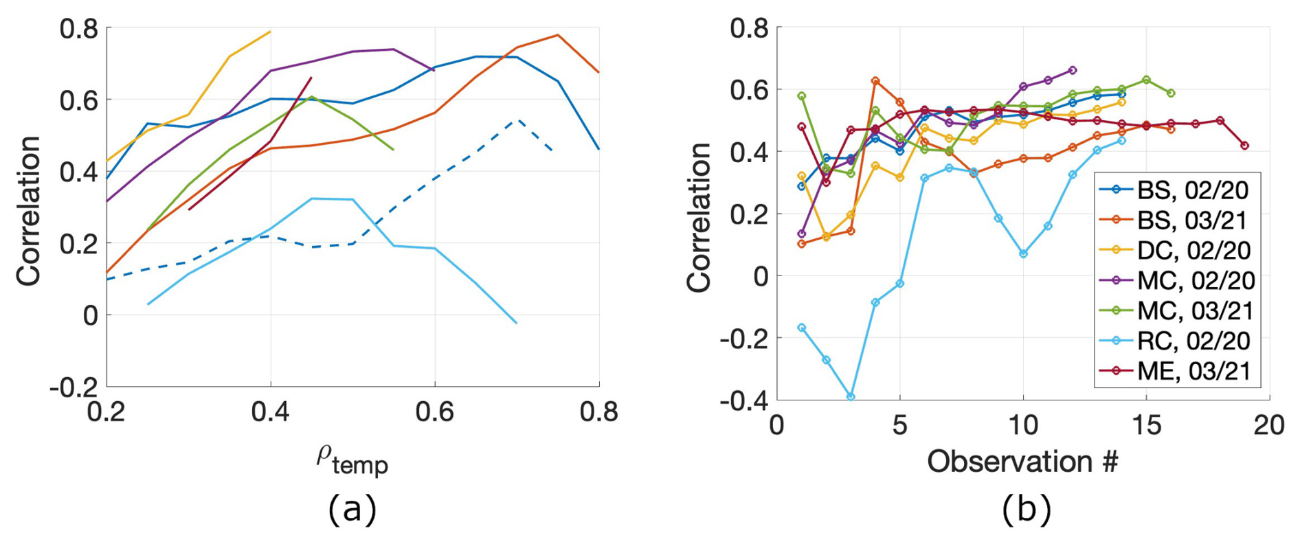
Figure 13 (a) Correlation between retrieved SWE using Sentinel-1 data and LIDAR snow depth versus average of Sentinel-1 temporal coherence. (b) Correlation between LIDAR snow depth and retrieved total SWE using Sentinel-1 on a specific observation date versus observation number. Different colors show the different LIDAR scenes.

Figure 13a shows the relationship between correlation and mean Sentinel-1 temporal coherence (ρ_temp) for sites with available 6 d repeat acquisitions. Different colors represent different LIDAR sites. As seen in the figure, the correlation generally increases with higher temporal coherence across most sites, with the exception of RC20. For example, in BS21 the overall correlation between retrieved SWE and LIDAR snow depth is 0.47 for the entire image, but ranges from ∼0.1 at low coherence to ∼0.78 at ρ_temp∼0.75. This pattern is consistent across most scenes, underscoring the critical role of temporal coherence in SWE retrieval: higher coherence enables more reliable phase measurements and, consequently, more accurate retrievals. At the same time, the presence of exceptions indicates that temporal coherence alone does not fully explain retrieval performance, and that additional environmental and observational factors must also be considered. Therefore, temporal coherence is used here as a primary metric for evaluating retrieval quality, while its interaction with other controlling parameters is examined in Sect. 5.1.1. Although TU21 exhibits a low overall correlation (0.13), Fig. 13a (blue dashed line) shows that correlation still rises to ∼0.5 in regions with higher temporal coherence. This demonstrates that reliable retrieval is possible even in generally low-performing sites when coherence is sufficiently high. However, because TU21 has low overall coherence across the scene, we exclude it from the parameter impact analysis. The exception is RC20, where temporal coherence does not improve retrieval performance. As discussed previously, this is likely due to frequent melt events and overall low SWE, which degrade retrieval accuracy despite coherence levels.

Figure 13b illustrates the correlation between retrieved SWE time series and LIDAR snow depth at the end of the time series. In most sites, correlations are relatively low early in the snow season but increase steadily, reaching near-maximum values between mid-January and early February, and attaining their highest values at the end of the time series. The fact that maximum correlation occurs at the LIDAR acquisition date indicates that the relationship is not random; rather, the correlation strengthens as the retrieval approaches the validation date. This trend also suggests that the primary spatial pattern of snow accumulation is largely established by February.

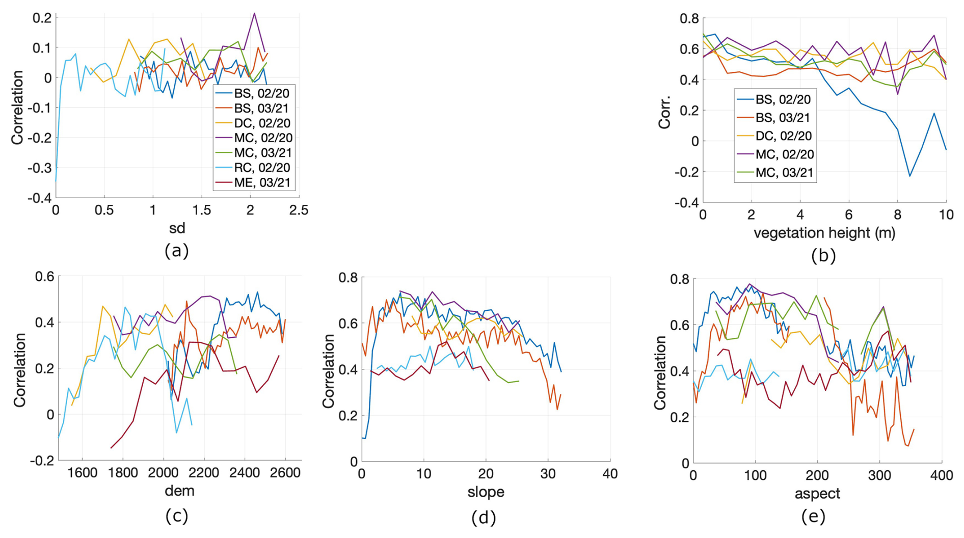
Figure 14 Correlation between retrieved SWE using Sentinel-1 data and LIDAR snow depth versus (a) snow depth (b) vegetation height (c) ground topography (d) ground slope (e) ground aspect. Different colors show the different LIDAR scenes.

Figure 14a–e illustrate the influence of snow depth, vegetation height, ground topography, slope, and aspect on the correlation between retrieved SWE and LIDAR snow depth. Different colors represent different LIDAR sites. Vegetation height is derived from the QSI LIDAR dataset, which provides co-registered measurements of vegetation structure and snow depth. Elevation is obtained from the Copernicus DEM (GLO-30), used within the ASF HyP3 processing workflow, with a spatial resolution of 30 m. Terrain slope and aspect are calculated from this DEM. All parameters are subsequently aggregated to match the 80 m spatial resolution of the multilooked Sentinel-1 data used in this analysis. Vegetation height data are only available for the QSI LIDAR products. As shown in Fig. 14a, total snow depth has little effect on retrieval performance. In contrast, Fig. 14b demonstrates that correlation decreases with increasing vegetation height, likely because vegetation obscures the snowpack and reduces retrieval accuracy. However, retrievals may remain reliable even in areas with tall vegetation, possibly due to canopy gaps or snow accumulation on top of the canopy. Correlation tends to increase with ground elevation within each site (Fig. 14c). However, this relationship is local rather than global; there is no specific elevation threshold beyond which performance improves uniformly. Instead, within a given site, higher elevations generally correspond to colder conditions, leading to drier snow and thus more reliable retrieval. As shown in Fig. 14d, correlation generally decreases with increasing ground slope, except in RC20 and ME21. Steeper slopes are expected to promote snow displacement, reducing temporal coherence and retrieval performance. However, RC20 and ME21 have relatively shallow snowpacks, which may limit downslope snow movement and explain the lack of slope dependence. Figure 14e shows that correlation is highest (except in RC20 and ME21) for aspect angles near 90°, corresponding to east-facing slopes. A possible explanation is that these slopes receive solar radiation earlier in the day, when temperatures are lower, thereby minimizing melt compared to west-facing slopes that receive afternoon sunlight under warmer conditions. In addition, as discussed in Sect. 4.1.2, observation geometry also contributes to this pattern. East-facing slopes tend to face toward the right-looking descending Sentinel-1 acquisition (6 am), resulting in higher backscatter, signal-to-noise ratio and improved temporal coherence. The combination of favorable viewing geometry and colder, drier snow conditions leads to improved SWE retrieval performance over east-facing slopes. In contrast, RC20 and ME21 exhibit consistently low correlations across all aspect angles, consistent with their shallow snowpack and warmer conditions.

5.1.1 Impact of Different Parameters on INSAR Temporal Coherence Using LIDAR Data

As discussed in Sect. 5.1, temporal coherence plays a critical role in SWE retrieval. To further investigate this, we evaluate the influence of different environmental parameters on temporal coherence over the LIDAR scenes. Since retrieval performance is very poor with 12 d repeat Sentinel-1 data, Sect. 5.1 considered only 6 d repeat acquisitions. Here, we assess parameter impacts separately for 6 and 12 d repeat data.

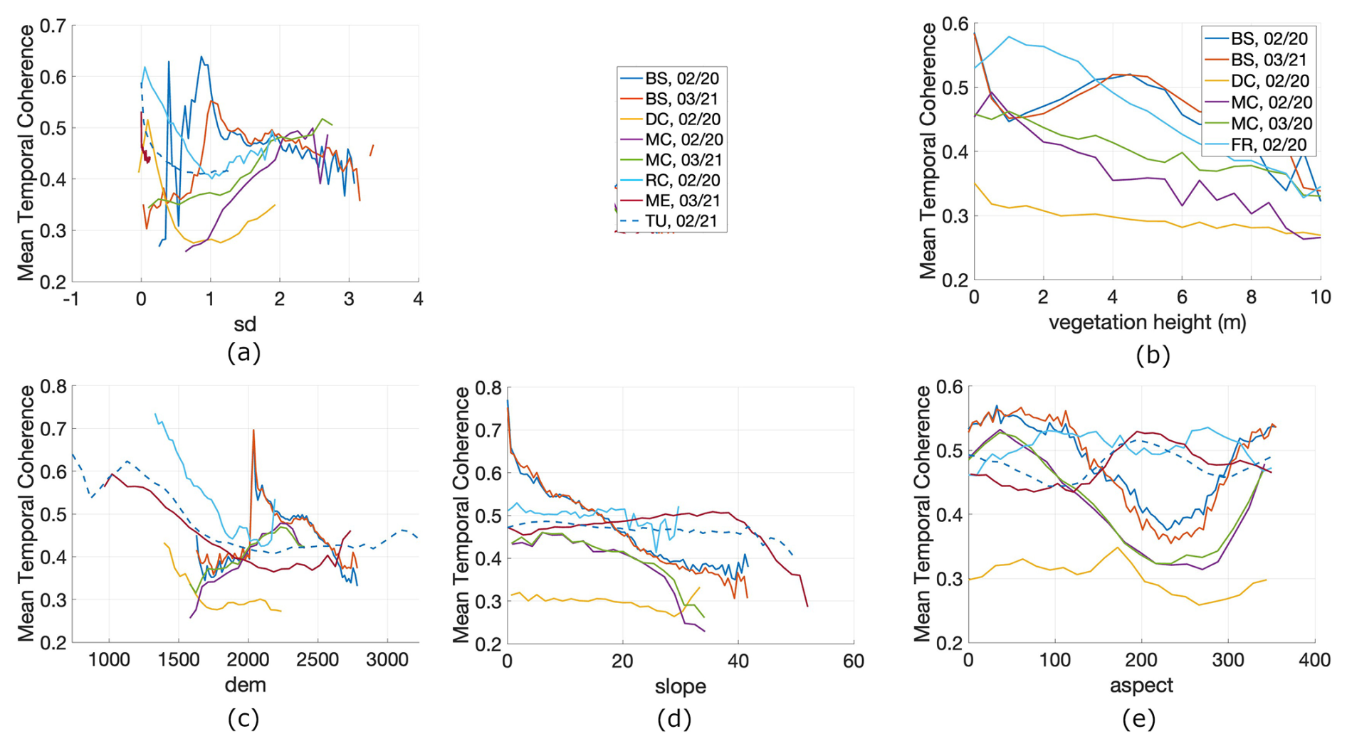
Figure 15 Average of Sentinel-1 temporal coherence versus (a) snow depth (b) vegetation height (c) ground topography (d) ground slope (e) ground aspect. Different colors show the different LIDAR scenes.

Figure 15a–e illustrates the effects of snow depth, vegetation height, elevation, slope, and aspect on Sentinel-1 temporal coherence, with different colors representing different LIDAR sites. The Sentinel-1 temporal coherence values shown in Fig. 15a–e are derived from 6 d repeat acquisitions. As shown in Fig. 15a, increasing snow depth generally reduces temporal coherence, except at the MC site. Deeper snow typically introduces more movement and structural change, lowering coherence. The anomalous behavior at MC remains unexplained. Notably, snow depth influences temporal coherence, whereas it showed little effect on correlation with LIDAR in Fig. 14a.

Figure 15b shows that temporal coherence decreases with increasing vegetation height, likely due to motion of leaves and branches. The impact of vegetation is stronger for temporal coherence than for correlation (cf. Fig. 14b). Temporal coherence also tends to decrease with elevation within individual sites (Fig. 15c). This relationship is site-specific rather than global: higher elevations often correspond to greater snow depth variability and wind exposure, which reduce coherence. Interestingly, topography exerts opposite effects on correlation and temporal coherence (Figs. 14c and 15c): higher elevations improve retrieval accuracy (drier snow) but reduce temporal coherence (increased snow depth change and wind).

As shown in Fig. 15d, coherence generally decreases with slope, consistent with the expectation that steeper terrain promotes snow displacement and reduces stability. RC20 and ME21 are exceptions, likely due to their shallow snowpacks, which limit slope-induced snow movement.

Aspect also plays an important role (Fig. 15e). Coherence is generally highest (except in ME21 and TU21) for east-facing slopes (∼90°) and lowest for west-facing slopes (∼270°). A possible explanation is that east-facing slopes receive solar radiation earlier in the day, under colder conditions, which reduces melt and preserves temporal coherence compared to west-facing slopes that experience warmer afternoon temperatures. In addition to these environmental effects, observation geometry also contributes to the observed pattern. For descending (6 am) Sentinel-1 acquisitions, east-facing slopes are oriented toward the radar line of sight, resulting in higher backscattered signal-to-noise ratio and consequently higher measured coherence. In contrast, west-facing slopes are more likely to face away from the sensor, leading to reduced backscatter and lower coherence. By contrast, ME21 and TU21 show the opposite pattern, with higher coherence on west-facing slopes, possibly due to site-specific wind conditions or local geometry effects.

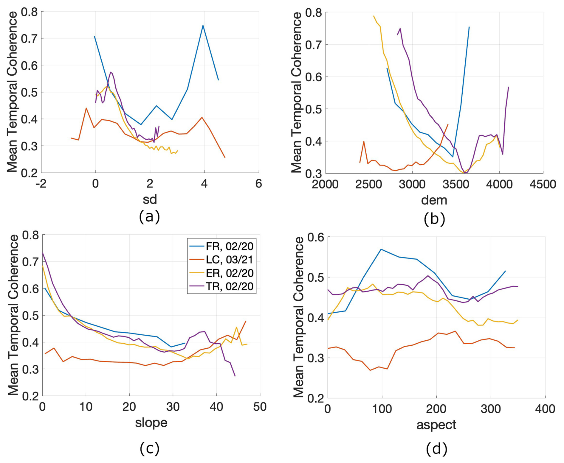
Figure 16 Average of Sentinel-1 temporal coherence versus (a) snow depth (b) ground topography (c) ground slope (d) ground aspect. Different colors show the different LIDAR scenes.

Figure 16a–d illustrates the influence of snow depth, elevation, slope, and aspect on Sentinel-1 temporal coherence using 12 d repeat data. The overall parameter dependencies are consistent with those observed for the 6 d repeat case (Fig. 15). However, coherence values are systematically lower for 12 d intervals, indicating that longer revisit times degrade temporal coherence even though the relative effects of the parameters remain similar.

5.2 Impact of Different Parameters on Retrieved SWE Using SNOTEL Data

In this section, we examine how different parameters affect the correlation between Sentinel-1-retrieved and SNOTEL ΔSWE using 6 d repeat acquisitions. We also assess the influence of these parameters on Sentinel-1 temporal coherence. In contrast to the site-specific validation in (Oveisgharan et al., 2024), this section leverages multi-site SNOTEL time series to investigate how environmental variability affects SWE retrieval performance and temporal coherence.

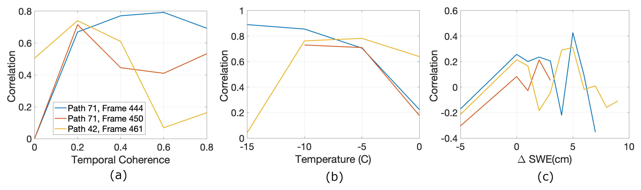
Figure 17 Correlation between retrieved ΔSWE using Sentinel-1 data and SNOTEL ΔSWE versus (a) Sentinel-1 temporal coherence (b) Temperature (°C) (c) ΔSWE.

Figure 17a–c illustrate the effects of temporal coherence, temperature, and ΔSWE on the correlation between retrieved and SNOTEL ΔSWE, with different colors representing individual Sentinel-1 frames. For each frame in Fig. 1b, we use the full time series of parameters and calculate the correlation for each subcategory. For example, in Fig. 1b the correlation between retrieved and SNOTEL ΔSWE is about 0.9 for all SNOTEL observations within the temperature range −15 to −10 °C in (p71, f444).

Figure 17a shows that the correlation between retrieved and SNOTEL ΔSWE increases with temporal coherence for (p71, f444), but decreases for (p71, f450) and (p42, f461). This behavior differs from the more consistent positive relationship observed between temporal coherence and performance in the LIDAR-based analysis (Fig. 13a), where higher coherence generally leads to improved agreement. It is important to distinguish between the two validation approaches used in this study, as they assess different aspects of retrieval performance. The SNOTEL-based analysis evaluates SWE change (ΔSWE) between individual interferometric acquisitions, and therefore reflects the temporal performance of the retrieval at specific time intervals. In contrast, the LIDAR-based analysis compares total retrieved SWE with total LIDAR-derived snow depth at a given date, which effectively integrates SWE changes over time and represents an aggregate measure of performance. As a result, the two approaches differ in their sensitivity to errors. In the LIDAR comparison, total SWE is obtained by summing ΔSWE over time. Any error in the reference point used for phase calibration propagates as a constant offset in the reconstructed total SWE. Such an offset does not affect spatial correlation with LIDAR snow depth, which primarily reflects the similarity of spatial patterns. In contrast, the SNOTEL-based analysis compares ΔSWE across multiple dates, and is therefore more sensitive to reference point errors and temporal noise. For example, estimating a small ΔSWE for large ΔSWE can significantly affect correlation with SNOTEL measurements, whereas in the LIDAR comparison the same error would contribute only a constant bias with no on spatial correlation. More broadly, the LIDAR-based analysis evaluates “spatial” correlation of “total SWE”, while the SNOTEL-based analysis evaluates “spatio-temporal” correlation of “SWE change”. Consequently, the relationship between temporal coherence and retrieval performance differs between the two approaches. In the LIDAR comparison, higher average temporal coherence over the time series generally leads to improved performance, as it reflects more reliable phase measurements accumulated over time. In the SNOTEL analysis, however, the relationship is more complex. High temporal coherence often occurs during periods of small ΔSWE, when retrieval performance is inherently more sensitive to noise and may degrade despite favorable coherence conditions. Therefore, the LIDAR-based analysis captures the integrated, average behavior of the retrieval, while the SNOTEL-based analysis reveals the instantaneous performance and its dependence on temporal variability. Together, these complementary perspectives provide a more complete understanding of the factors controlling SWE retrieval performance. If a temporally consistent LIDAR time series were available, co-registered with the InSAR acquisitions, the comparison would become more analogous to the SNOTEL-based analysis, as both would involve evaluating SWE and snow depth changes between acquisition dates and their dependence on temporal coherence. In that case, the relationship between coherence and retrieval performance would be expected to follow similar behavior to that observed in the SNOTEL comparison.

As expected, higher temperatures reduce retrieval performance, as shown in Fig. 17b. Warmer conditions promote melt, which lowers the correlation between retrieved and SNOTEL ΔSWE, consistent with the behavior reported in (Ruiz et al., 2022). In contrast, the magnitude of SWE change does not significantly impact correlation, as shown in Fig. 17c.

Figure 18 Average of Sentinel-1 temporal coherence versus (a) temperature (°C) (b) ΔSWE.

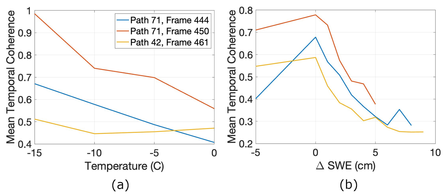
We also evaluate the influence of temperature and SWE change on temporal coherence using SNOTEL data. Figures 18a and 13b show that temporal coherence decreases with increasing temperature and with larger ΔSWE. Higher temperatures make the snow wetter and increase snow particle motion, reducing coherence. Similarly, larger SWE changes are often accompanied by strong winds and substantial modifications to the scattering medium, which also degrade temporal coherence. This study moves beyond demonstrating the feasibility of InSAR-based SWE retrieval by providing a systematic evaluation of its performance across varying environmental conditions. The results identify the dominant controls on retrieval accuracy and define the conditions under which the method is reliable, which are critical steps toward operational SWE monitoring using current and future SAR missions.

6 Conclusions

This study evaluated the performance of Sentinel-1 repeat-pass interferometry for estimating snow water equivalent (SWE) across multiple SnowEx sites using coincident airborne LIDAR and SNOTEL datasets.

While previous work demonstrated the feasibility of SWE retrieval using Sentinel-1 interferometry, this study provides the first comprehensive, multi-site evaluation of retrieval performance and its controlling factors. By quantifying the roles of temporal coherence, temperature, vegetation, and terrain, we establish the conditions under which InSAR-based SWE retrieval is reliable, representing a key step toward large-scale and operational applications. These results also provide a foundation for quality assurance (QA) in future SWE products by identifying the key parameters that control retrieval reliability and uncertainty. Results confirm that the 6 d Sentinel-1 acquisitions coordinated with the SnowEx campaign substantially enhance temporal coherence and improve SWE retrieval performance relative to the standard 12 d repeat. The correlation between Sentinel-1-retrieved SWE and LIDAR snow depth ranges from 0.42 to 0.66 across sites, with the strongest agreement observed in cold, dry regions exhibiting stable snowpacks. Similarly, correlations between retrieved and SNOTEL SWE change reach 0.81, with corresponding RMSE values below 1 cm. Our analysis suggests that temporal coherence is one of the primary factors influencing retrieval accuracy. Coherence decreases with increasing snow depth, slope, vegetation height, temperature, and SWE change, indicating that snow metamorphism, melt events, and surface motion are primary sources of decorrelation. Reliable retrievals are achieved primarily under cold, dry-snow conditions and in relatively flat, sparsely vegetated terrain. While 12 d revisit intervals result in severe coherence loss, the 6 d repeat provides sufficient temporal stability for C-band SWE retrieval in many mountain environments. In contrast, longer wavelengths such as L-band are intrinsically less sensitive to small-scale scattering changes and therefore maintain higher temporal coherence over longer revisit intervals. As a result, missions such as NISAR are expected to enable robust SWE retrieval despite a 12 d repeat cycle, while also benefiting from reduced phase ambiguity. These findings validate the feasibility of C-band InSAR for quantitative SWE mapping and provide insight into the environmental and observational constraints governing retrieval performance. The framework and analyses developed here directly inform the application of upcoming L- and S-band missions such as NISAR, which will extend InSAR-based SWE retrievals to global scales with improved coherence and temporal sampling.