First arctic-wide assessment of SWOT swath altimetry with ICESat-2 over sea ice

This study presents an Arctic-wide assessment of the Surface Water and Ocean Topography (SWOT) mission's swath observations of sea surface height (SSH). SWOT provides measurements in two-dimensional swaths and enables pixel-based height information with a resolution of 250 m up to a latitudinal limit of 78° N. Although SWOT doesn’t cover the central Arctic, it provides insights into SSH at an unprecedented spatial and temporal resolution. The quality of these innovative observations in such a challenging environment is evaluated through comparison with data from ICESat-2. Approximately one year of surface elevation data, collected between March 2023 and April 2024, is used at around 550 regionally distributed crossover locations, with measurements taken within 30 min. Sentinel-1 SAR imagery supports the comparisons if available. Visual comparisons of SWOT and ICESat-2 with Sentinel-1 backscatter (i.e. σ₀), converted to 8-bit grey-scale values, reveal clear coherence. However, small-scale surface features aren’t captured by SWOT as equally as by ICESat-2. The data shows absolute water level differences of about 5 cm, despite prior harmonisation of references and corrections. Differences of up to 50 cm can occur when comparing left- and right-hand SWOT swaths, mainly during winter and in areas with long sea ice coverage. This may be due to issues with the height correction from the crossover calibration. Quantitative point-by-point comparisons show mean standard deviations of about 8 cm for all surface types and 6 cm if restricted to ICESat-2-detected leads. Higher deviations are found during the early melting period between May and June, in the Canadian Archipelago and the Greenland Sea.

1 Introduction

The Surface Water and Ocean Topography (SWOT) mission was launched in December 2022. SWOT, an innovative altimeter mission operated by NASA and CNES, supported by the Canadian Space Agency and the UK Space Agency, has the primary objective of monitoring terrestrial water heights and the ocean surface with high spatial resolution. The unique novelty of SWOT is the use of a K_a-band SAR radar interferometer (KaRIn) with near-nadir incidence angles between 0.6 and 3.9°. KaRIn does not sample the sea surface in nadir, but provides sea surface elevations within a 60 km left and right swath (Morrow et al., 2019). It is the first altimetry mission, which provides 2D samples of the ocean topography. Moreover, SWOT's promising observations have motivated future missions, such as the upcoming Copernicus mission Sentinel-3 Next Generation Topography (S3NG-T). This mission, planned for launch after 2030, will adopt the swath altimetry concept and bring it to an operational level. It will consist of two satellites, each carrying an across-track interferometer and a nadir-looking synthetic aperture radar (SAR) altimeter. The results of this study will help to prepare for this future mission.

SWOT's orbital configuration makes it possible to cover large parts of the Arctic (up to 77.6° N) and the entire Southern Ocean. Even though SWOT was not primarily designed as an ice mission, it opens up new possibilities for investigating the polar oceans with regard to sea ice drift, open water detection, sea level and freeboard determination. The mission provides data with different spatial resolutions, ranging from tens of meters at the High-Rate (HR) up to approximately 500 meters (i.e., 250 m pixel posting rate) in the Low-Rate (LR) mode and allows for the detection of ice floes and leads (i.e., elongated water openings within the sea ice) of different size.

Before using the SWOT data for scientific analyses, it should be validated in order to retrieve information on precision and possible systematic errors. This is particularly important because of SWOT's completely new measurement principle. Since in-situ data in the Arctic is rare and not available over wide areas, one way of assessing the SWOT data quality is to compare it with data from other satellite missions, for example, with surface height measurements from ICESat-2 laser altimetry.

ICESat-2, NASA's Ice, Cloud, and Land Elevation Satellite (Neumann et al., 2019) launched in 2018, carries a photon-counting laser altimeter and is characterized by a dense observation sampling and the ability to monitor very precisely fine-scale surface changes in polar regions. ICESat-2 aims to monitor ice sheet melting, detect ridges and provide information about surface roughness. Moreover, ICESat-2 provides the opportunity to observe small-scale features of the sea ice surface, for example small leads or water openings within the sea ice cover to support sea ice freeboard or thickness computations (e.g., Farrell et al., 2020; Kacimi and Kwok, 2022; Petty et al., 2023; Ricker et al., 2023)

In general, there is very little published work using SWOT in the polar regions. Armitage and Kwok (2021) used simulated SWOT data as well as precipitation measurements and K_a-band nadir altimetry to analyse SWOT-like backscatter histograms during sea ice conditions. Most recently Kacimi et al. (2025) published an initial comparison of SWOT swath-altimetry with two selected overlapping ICESat-2 tracks within the Weddell and the Beaufort seas in terms of backscatter, SSH, and freeboard heights.

Our study presents an assessment of SWOT-KaRIn surface heights in the Arctic sea-ice regions. Due to a lack of sufficient in-situ data, a comparison with ICESat-2 laser altimetry is performed. Besides an Arctic-wide assessment, we cover a long period of time, including different seasons and both SWOT orbit phases. With this, we extend the work of Kacimi et al. (2025). The comparison is based on 550 suitable crossovers between both missions with short acquisition time differences of maximum 30 min to minimize the impact of sea ice drift and re-freezing of leads due to rapid and abrupt temperature changes. Where possible, radar images from ESA's Corpernicus Sentinel-1A (S1) mission are additionally used as background data with pixel resolutions of 25 or 40 m. For this purpose, dual-polarized SAR images are processed by using the SNAP (ESA Sentinel Application Platform v9.0.0 http://step.esa.int, last access: 14 January 2026) toolbox as described in Müller et al. (2023) to generate HH-polarized 8-bit grey-scaled backscatter (i.e. σ₀) SAR images.

After a discussion of the advantages and challenges of the current SWOT data product based on selected crossover examples, we quantify the accuracy of the height measurements on the basis of all differences at the intersection points. Using statistical methods on the basis of 550 crossover spots from March 2023 until April 2024, we analyse systematic errors as well as the precision of the SWOT measurements.

2 Data

2.1 SWOT

Two different observation modes are available for SWOT in the Arctic Ocean. The low rate (LR) mode is mainly limited to ocean areas and is the predominant observation mode. The high rate (HR) mode is available in coastal and inland areas, but also seasonally between December and February in an area of about 220 000 km² in the Beaufort Sea. Both observation modes provide pixel-based and gridded height information, but are made available as different products. In this study, surface elevation information is obtained from the Level-2 (L2) LR Unsmoothed KaRIn data set for the cal/val (1 d repeat) and science (21 d repeat) phase with an effective spatial resolution of approximately 500 m (JPL D-56407 Revision B, 2023). By default the L2 LR Unsmoothed data is provided on a spatial grid of 250 m resolution and is made available through the NASA Physical Oceanography Distributed Active Archive Center (PO.DAAC; SWOT, 2024). In terms of available data releases, Version C of the latest reprocessed PO.DAAC data (i.e., “PGC”) is used. For nearly half of the science phase, files of the forward precessing (i.e., “PIC”) are used since no reprocessed product was yet available.

Surface elevation observations are taken from ssh_karin_2 for left and right swath observations. These heights are already corrected by model-based delays for the dry and wet troposphere and the ionosphere, as well as for the sea state bias. Missing corrections for tides, i.e. solid Earth tides (SET), pole tides (PET) and ocean tides (OT), and the Dynamic Atmosphere Correction (DAC) are obtained from the SWOT L2 Expert product (JPL D-56407 Revision B, 2023). The same applies to the so-called L2 calibration correction (COR; i.e. height_cor_xover) required to reduce systematic height errors in the elevation measurements of KaRIn. It is computed by performing a crossover analysis of ascending and descending SWOT tracks (Dibarboure et al., 2022). In summary, surface height (SH) from SWOT is computed as followed:

$$\begin{array}{}\text{(1)}& \mathrm{SH}=\mathrm{ssh}\mathit{\_}\mathrm{karin}\mathit{\_}\mathrm{2}-(\mathrm{SET}+\mathrm{PET}+\mathrm{OT}+\mathrm{DAC})+\mathrm{CAL}\end{array}$$

Since the corrections from L2 Expert files are sampled on a 2 km grid, they are bi-linearly interpolated to the Unsmoothed grid nodes and applied to ssh_karin_2. For more details on the applied corrections, we refer to the dataset documentation of L2 LR SSH Unsmoothed and Expert in JPL D-56407 Revision B (2023). In order to derive anomalies of the surface elevation observed with respect to a reference surface, the DTU21MSS (Andersen et al., 2023) mean sea surface, available in a 1 min ° resolution, is interpolated and subtracted from the corrected SH. The computation takes into account flags, included in the SWOT data, in order to exclude observations that are of poor (i.e. invalid) quality. ssh_karin_2 data labelled as bad_not_usable and bad values of height_cor_xover flagged in height_cor_xover_qual are rejected. However, data is used that is flagged as suspect (i.e off-nominal value, but might be useful), as this flag applies to almost the entire sea-ice region (see Fig. 1).

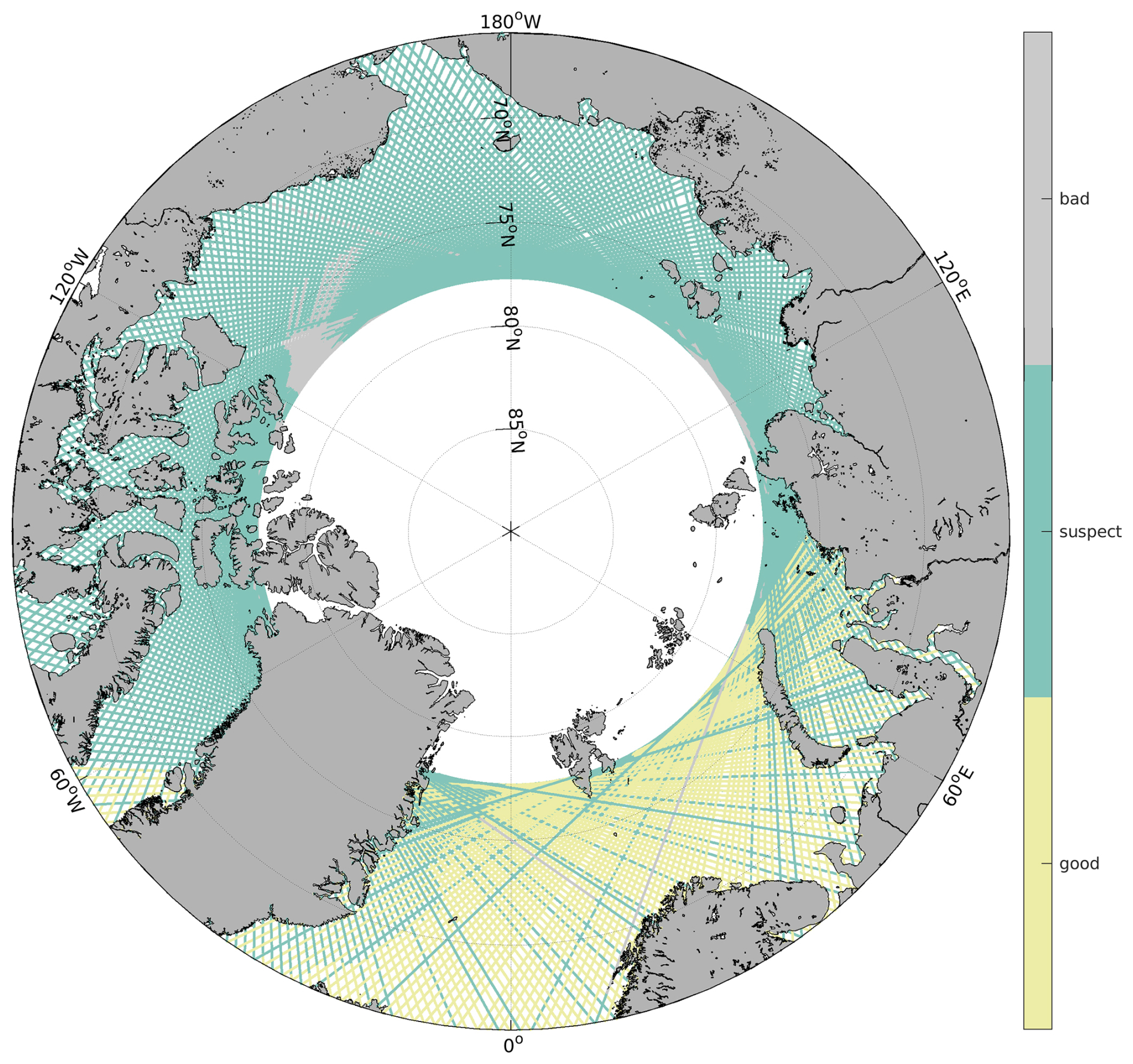
Figure 1 Overview of the L2 Expert quality flag of the height correction from the crossover calibration (height_cor_xover_qual) for January 2024 projected to the nadir altimeter position.

To enable a point-wise comparison with ICESat-2, surface elevations from SWOT are bi-linearly interpolated to the individual ICESat-2 laser beam crossing positions for the left and the right swath, respectively. Data are removed as outliers based on an along-beam moving standard deviation with an outlier criterion based on an interquartile range of 1.5 times above the 75 % percentile and below the 25 % percentile on the interpolated SWOT observations. Moreover, to minimise the effect of incorrectly increased height values at the swath edges, data within a 5 km distance to the outer and inner edges of the SWOT swaths are removed from the statistical comparisons (see Sect. 3).

2.2 ICESat-2

ICESat-2 samples the ocean topography in a particular dense observation pattern due to a laser beam split into 6 individual beams, a small footprint size of 11 m (Magruder et al., 2020), a high measurement frequency of 10 kHz (i.e. 70 cm observation point distance) and a 91 d orbit repeat cycle (Neumann et al., 2019).

ICESat-2 latest surface elevation segments from ATL07 Release 006 (Kwok et al., 2023) are used for this study. The ATL07 product covers the polar, ice-covered oceans of the Earth. It stores along-track surface heights of leads and sea ice for all areas with sea ice concentrations of more than 15 % (Kwok et al., 2023) for all 6 ground tracks (gt). Depending on the number of reflected photons, which is influenced by the surface reflectivity and cloud conditions, the spatial sample point resolution or height segment distance is variable. It ranges typically from 15 to 30 m (Ricker et al., 2023) with a maximum of 150 m. For the comparison with SWOT KaRIn observations, ICESat-2 elevations are utilised with and without the application of sea-ice/lead flagging in order to facilitate a comparative assessment of ATL07 heights for both surface types. Only ICESat-2 observations from the 3 strong beams are used for statistical and quantitative analyses, because minimal elevation differences and resulting slopes between strong and weak beams are closer together than the spatial resolution of SWOT.

Before comparing surface heights from ICESat-2 with KaRIn swath observations, the stored ICESat-2 elevations in height_segment_height must undergo some pre-processing steps to allow for consistent comparisons. Therefore, the mean sea surface used specifically for ICESat-2 (MSS13; Kwok et al., 2020) is replaced by DTU21MSS (Andersen et al., 2023), and the applied dynamic inverted barometer correction (DynIB) is substituted by DAC. Furthermore, the provided surface elevations are converted into a mean-tide reference by adding a geoid free-to-mean conversion factor (MT_factor). As a result, the ICESat-2 surface heights are calculated as follows:

$$\begin{array}{}\text{(2)}& \begin{array}{rl}\mathrm{SH}& =\mathrm{height}\mathit{\_}\mathrm{segment}\mathit{\_}\mathrm{height}+\mathrm{MSS}\mathrm{13}+\mathrm{DynIB}\\ & -\mathrm{DAC}+\mathrm{MT}\mathit{\_}\mathrm{factor}\end{array}\end{array}$$

With the exception of the introduced DTU21MSS, all corrections and conversions are included in ATL07 (Kwok et al., 2023). See the Algorithm Theoretical Basis Document for Sea Ice Products in Appendix J (Kwok et al., 2022) for more information on the replaced corrections.

The along-track ICESat-2 surface elevations are filtered by applying a standard Grubbs outlier flagging per laser beam (Grubbs, 1950). Afterwards, they are smoothed by a moving rectangle filter considering the effective SWOT Unsmoothed pixel resolution of 500 m (JPL D-56407 Revision B, 2023).

2.3 Overlaps

The comparison between SWOT and ICESat-2 is performed in the Arctic Ocean between 66 and 78° N. Crossovers between both missions are defined when the acquisition time differs less than 30 min. This time interval provides a good compromise between data availability and minimization of influences on the observation scenario due to sea ice drift and rapid temperature changes (Müller et al., 2023). To search for these crossover locations, the nominal nadir altimeter ground tracks of the cal/val and science orbit of SWOT are intersected with the nominal middle ground track (i.e. gt2) of ICESat-2 over the period between 30 March and 10 July 2023 as well as 26 July 2023 and 30 April 2024. This leads to a theoretical availability of around 288 comparison spots (all laser beams combined) during cal/val and 640 during the science phase, marked with a cross in Fig. 2. While most crossover locations are found in the Arctic peripheral seas, almost no comparisons are available in the eastern Greenland Sea and the Barents Sea due to a lack of sea ice coverage (< 15 % sea ice concentration). Moreover, there are fewer to no usable overflights in the months of August to November due to data gaps during the transition from the SWOT cal/val phase to the scientific phase. In March 2024, there are no overlaps within 30 min due to the orbit configuration of ICESat-2 and SWOT. Further, the number of crossovers used is reduced by applying a minimum comparison observation number of 500 per swath (left/right) and performing the outlier rejection on the SWOT and ICESat-2 surface elevations as described in Sect. 2.1 and 2.2 for minimizing the influence of outliers on the statistical analyses (see red dots Fig. 2). After performing the outlier rejection, observation points at 550 crossover locations remain for use in a visual and statistical comparison. The area of a crossover spot (and thus the length of the ICESat-2 ground track used for comparison) varies, since it depends on the geographical latitude and the angle at which the two satellite missions intersect.

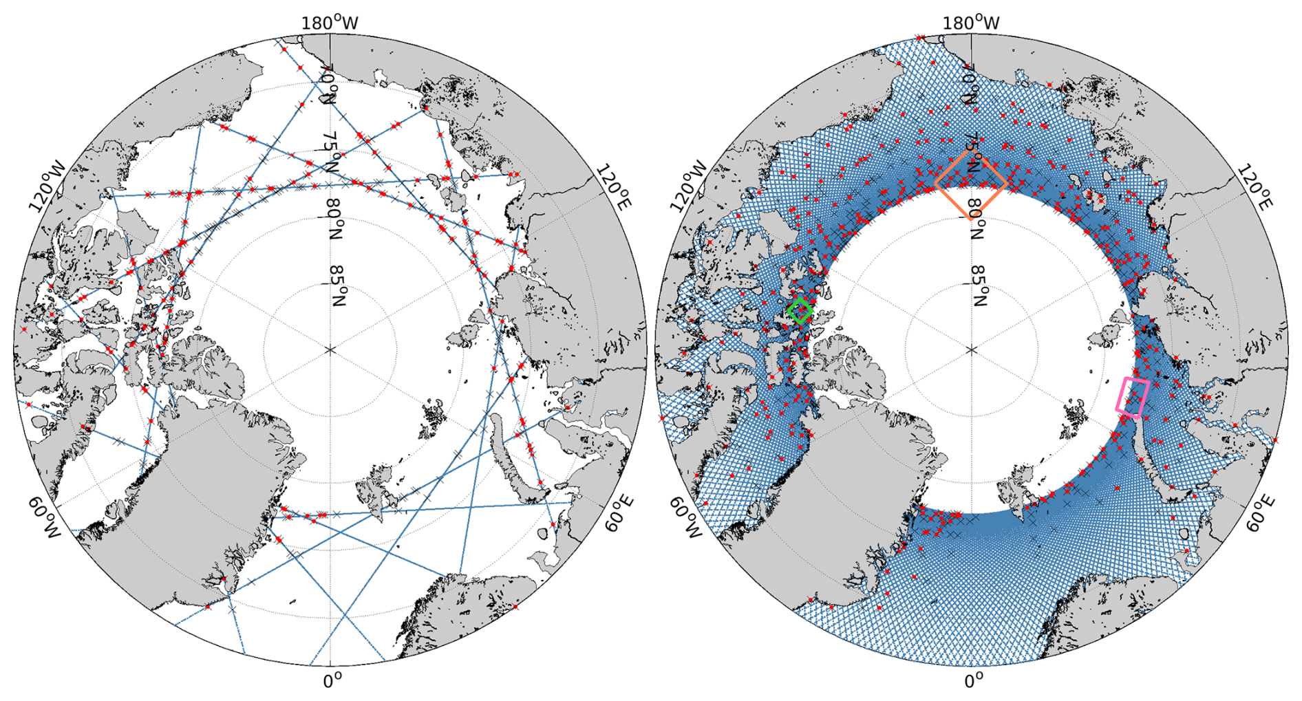
Figure 2 SWOT ground tracks in the Arctic (blue lines) for the SWOT cal/val phase (left) and the science phase (right). Theoretically usable crossovers between SWOT and ICESat-2 ground tracks considering land-water mask flagging and suitable cloud conditions marked with black crosses X, (#288 cal/val; #640 science) and effectively used crossover locations (red dots, #147 cal/val; #400 science) considering a 30 min time interval between both observations. Coloured rectangles show the areas of the compared examples (see following sections).

3 Comparison and results

Prior to the quantitative assessment of the SWOT data, visual comparisons between the three sensors of SWOT, ICESat-2 and Sentinel-1 are carried out for selected examples. This is done in order to demonstrate the potential of SWOT to represent small-scale surface types such as ice floes or leads. The SWOT surface elevations are compared to ICESat-2 surface heights as well as to the Sentinel-1 SAR image backscatter converted to grey-scale values. In sea ice areas, the SAR image backscatter is mainly controlled by the surface roughness, but also by height and sea ice topographic variations. Leads or open water patches usually tend to appear very dark in SAR images (low backscatter) due to mirror-like scattering characteristics. In contrast, rough sea ice surfaces or topographic features like ridges or hummocks for example result in stronger backscatter due to a more diffuse backscattering (e.g. von Albedyll et al., 2024, Murashkin et al., 2018, Dierking, 2013). This three-sensor comparison offers the possibility to uncover differences and similarities with regard to different surface types in addition to the direct comparison of along-track elevations.

Figure 3 shows an example of a SWOT – ICESat-2 crossover in the northern Kara Sea, near Novaya Zemlya Island. Sea ice surfaces and detached ice floes show up in the SWOT swath data mostly as elevations in relation to the lower lying leads and open water patches. Towards the outer edges of the swaths, especially in the last 5 km (both far-range and near-range), increased, dominant noise and erroneous surface heights become visible. These areas are thus excluded from the quantitative analysis (see Sect. 2.1). Additionally, artifact-like structures are observed near the island's coastline. Besides these deficiencies, the surface elevations observed by ICESat-2 and SWOT show similar variabilities, particularly in the three narrow, lead-shaped structures (highlighted area).

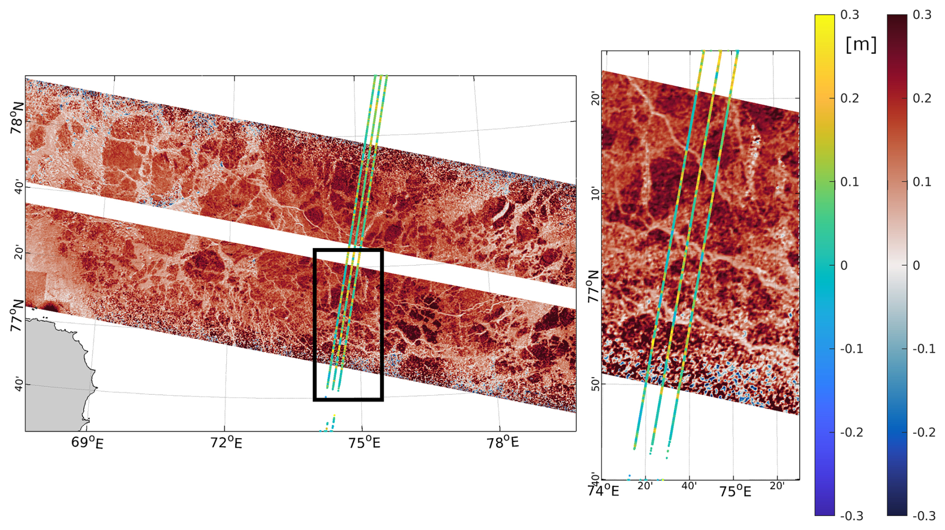
Figure 3 Example of SWOT swath (blue to red colorbar) and ICESat-2 (rainbow coloured) surface height observations (left) and zoom (location indicated by black box) on southern SWOT swath (right) on 23 January 2024 in the Kara Sea (see Fig. 2 pink rectangle) without subtraction of absolute mean values and the treatment of outliers at the swath edge. Acquisition time differences: SWOT vs. ICESat-2, 13 min.

Figures 4 and 5 illustrate the inter-comparison between SWOT, ICESat-2 and Sentinel-1 in January 2024 in the Canadian Archipelago. In this context, the SAR image is only used as a qualitative indicator to support the comparison between SWOT and ICESat-2. While the first figure shows the geographical map, the second one displays the interpolated along-track heights. The Sentinel-1 grey-scaled backscatter values show a strong coherence with SWOT and ICESat-2 surface elevation variations. The comparison of the 3 strong laser beams and the Sentinel-1 grey-scaled backscatter values clearly reveals that the surface profile consisting of different sea ice surface types is captured quite well by SWOT. This applies in particular to distinct surface features, such as wide leads, that are characterised by low Sentinel-1 grey-scaled backscatter values or larger ice floes featured by brighter grey-scaled backscatter values (e.g. in Fig. 5 highlighted in orange), which are sampled similarly to ICESat-2 in terms of height. Even smaller features, such as a lead in the right swath (zoom Fig. 4 bottom left), can be monitored very well by SWOT and ICESat-2. A closer look at an ice floe with a diameter of about 3.5 km, which is cropped in Fig. 4 bottom right, shows that SWOT, similar to overlapping ICESat-2 beams, is able to detect small height differences within the ice floe surface.

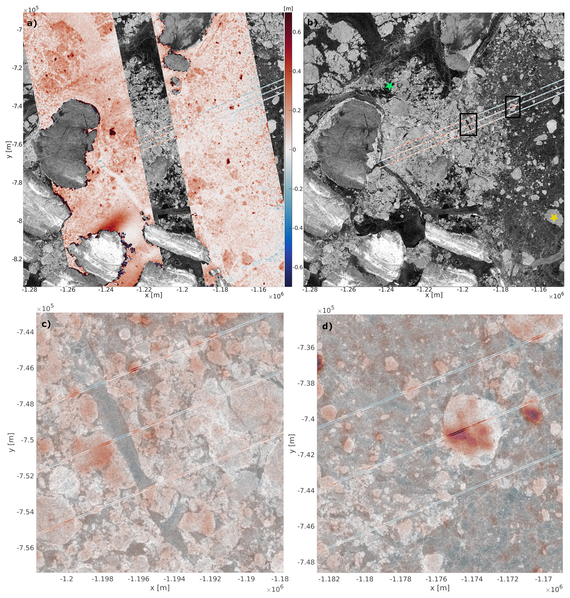
Figure 4 Example of SWOT swath surface elevations, ICESat-2 profiles (in meter) and Sentinel-1 (gray-scale) image on 25 January 2024 in the Canadian Archipelago (see Fig. 2 green rectangle) with SWOT (a) and without SWOT (b). The stars indicate regions that are discussed in the text. Bottom row shows two detail views (c, d) with backgrounded SAR backscatter (in grey-scale values) information (locations are indicated with black boxes in b). Geographical coordinates are stereographic north projected (EPSG:3413). Acquisition time differences: SWOT vs. ICESat-2, 5 min.; SWOT vs. Sentinel-1, 60 min.

However, as can be seen from Fig. 4, the height determination outside the ice floe is dominated by noise, and clear elevation signatures cannot be clearly recognized or assigned to ocean topography. Further inconsistencies between elevation changes from SWOT and ICESat-2 are apparent in regions with smaller ice floes close to the coasts or in the vicinity of small islands. In some regions, certain sea ice surfaces visible in the radar image are apparently not represented in the SWOT elevations or do not have a particular elevation signature compared to other sea ice areas. This is evident, for example, in Fig. 4 in the left swath, green star, and at the right SAR image edge, orange star, where an ice floe shows nearly no height difference relative to the surrounding water. This suggests that small-scale height variations are smoothed stronger by SWOT compared to ICESat-2, as can be seen particularly clearly in Fig. 5 (bottom/middle row marked in red).

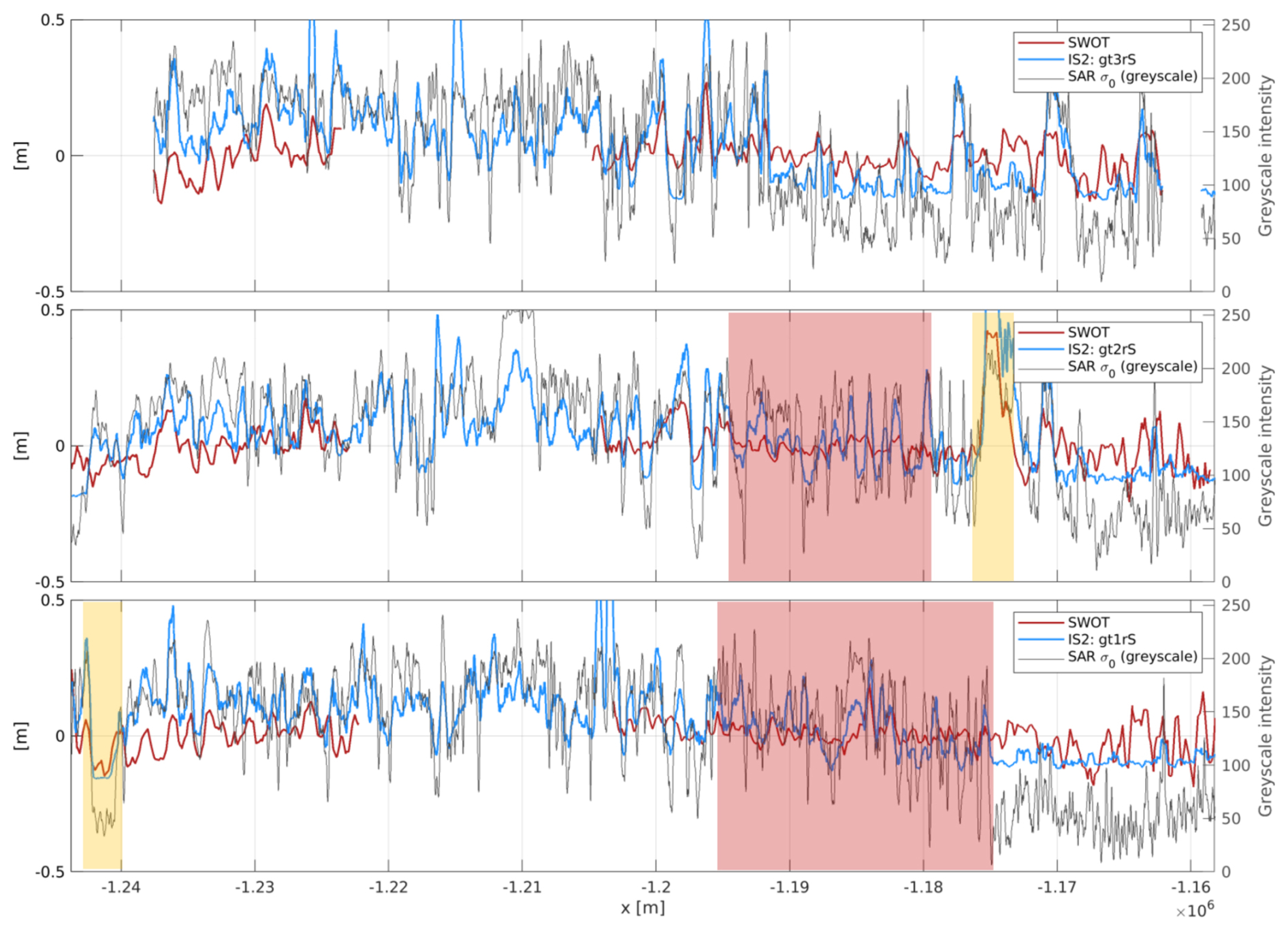
Figure 5 Along-track height comparisons in the Canadian Archipelago (same area as in Fig. 4) for the three strong beams of ICESat-2 (blue). Interpolated SWOT heights in red and Sentinel-1 backscatter image converted to grey-scale values in grey (right axis). Orange highlighted sections show lead and floe areas; red areas show clearly dampened height variations of SWOT compared to ICESat-2. Note: Along-track height observations are zero-centred by reducing the mean per ground track (gt) and swath side.

A further challenge in the swath surface height determination arises when leads are covered by thin sea ice or frost flowers or are exposed to strong winds, roughening the water surface. In the case of Sentinel-1, such conditions can cause strong backscatter (i.e. bright grey-scale values), which usually represents sea ice ridges, but can also indicate leads (Müller et al., 2023; Murashkin et al., 2018). In the SWOT elevation data, these bright patterns do not always appear to lie lower than the surroundings, but are sometimes significantly higher. This effect is particularly evident in areas where potential leads or ridges show different heights in the intersection points. Figure 6 shows some examples of this effect (see purple arrows).In the Chukchi Sea region in January 2024, an almost homogeneous sea ice surface is visible, only interrupted by some leads or ridges, which cause distinct height signatures in the SWOT elevations. However, the observed surface elevations cannot always be unambiguously attributed to the correct surface type (i.e., clearly defined as a lead or a ridge). The full explanation of what directly causes these uncertainties remains unclear. Rather, the structure orientation (i.e., the striking) also appears to have an influence on the observed elevation differences. Additionally, this example shows large systematic cross-track errors of almost 50 cm. Probably the height correction from the crossover calibration (i.e. height_cor_xover) is insufficient or error-prone over almost closed sea ice areas, as no direct crossover adjustment can be conducted under these conditions (Dibarboure et al., 2022). Unfortunately, the available height calibration quality flag does not help here, since sea ice areas are entirely marked as “suspect” (see Fig. 1 exemplary for January 2024). A rejection of “suspect”-labelled crossover height calibration would result in excluding all SWOT observations during sea ice conditions.

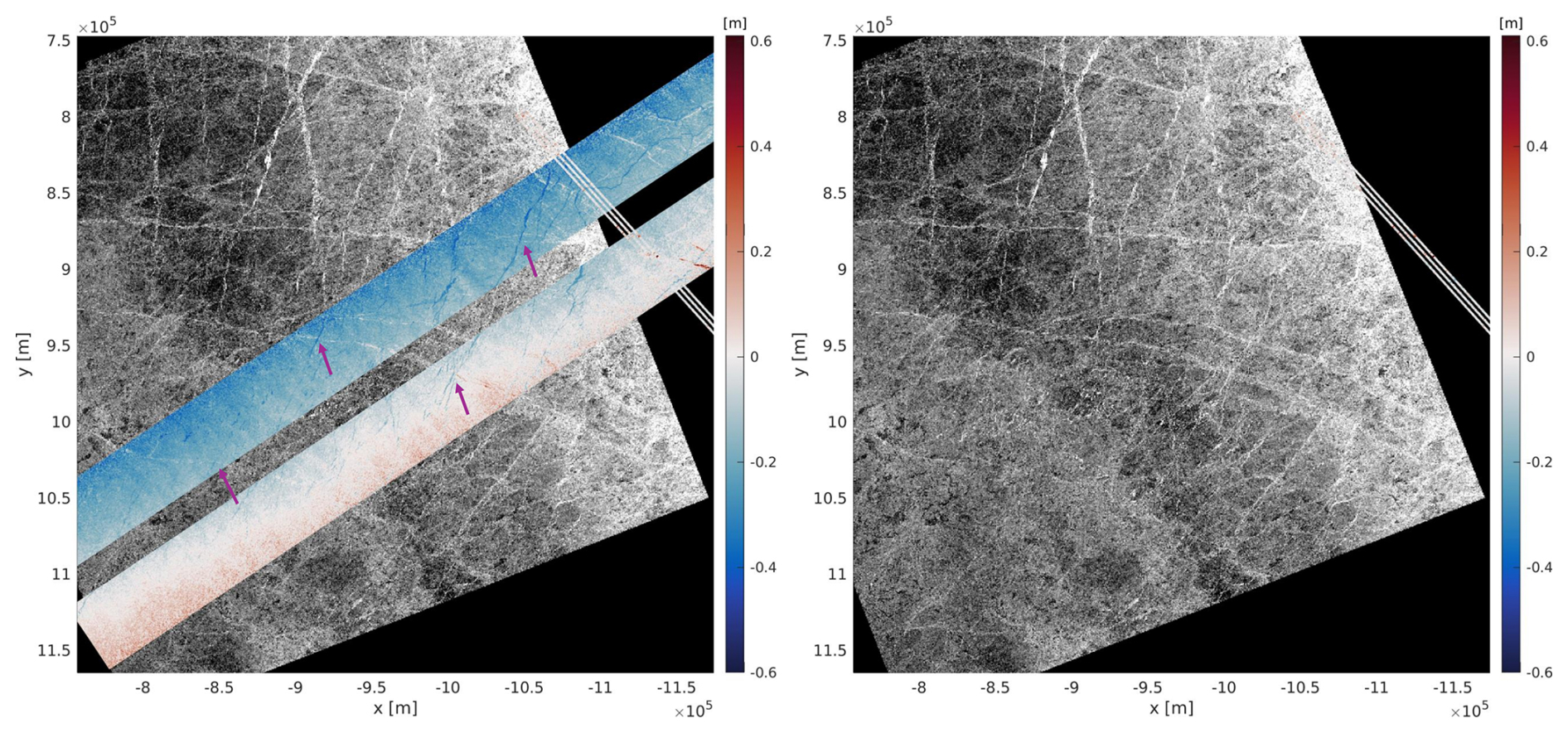
Figure 6 Example of coloured SWOT surface elevation swath, ICESat-2 profiles and a Sentinel-1 image (left) and without SWOT for comparison (right) on 21 January 2024 in the Chukchi Sea (see Fig. 2 orange rectangle). Arrows indicate lead/ridge regions that are discussed in the text. Geographical coordinates are stereographic north projected (EPSG:3413). Acquisition time differences: SWOT vs. ICESat-2, 20 min.; SWOT vs. Sentinel-1, 38 min.

In order to extend the assessment, a quantitative analysis of coincident SWOT and ICESat-2 surface elevation observations is performed. For this purpose, ICESat-2/SWOT crossovers during SWOT's cal/val and science period with a minimum of 15 % sea ice coverage (Kwok et al., 2023) have been used.

First, mean values of the ICESat-2 laser observations and the interpolated SWOT data per left and right swath have been computed. The means are shown as scatter plots in Fig. 7 for the left and for the right swath. There is generally good agreement with a correlation of about 74 % for the left and 69 % for the right swath. The fact that the differences are not normally distributed, but have two maxima (at least in the left swath), indicates that this is due to systematic errors in some overflights, probably caused by incorrect cross-calibration.

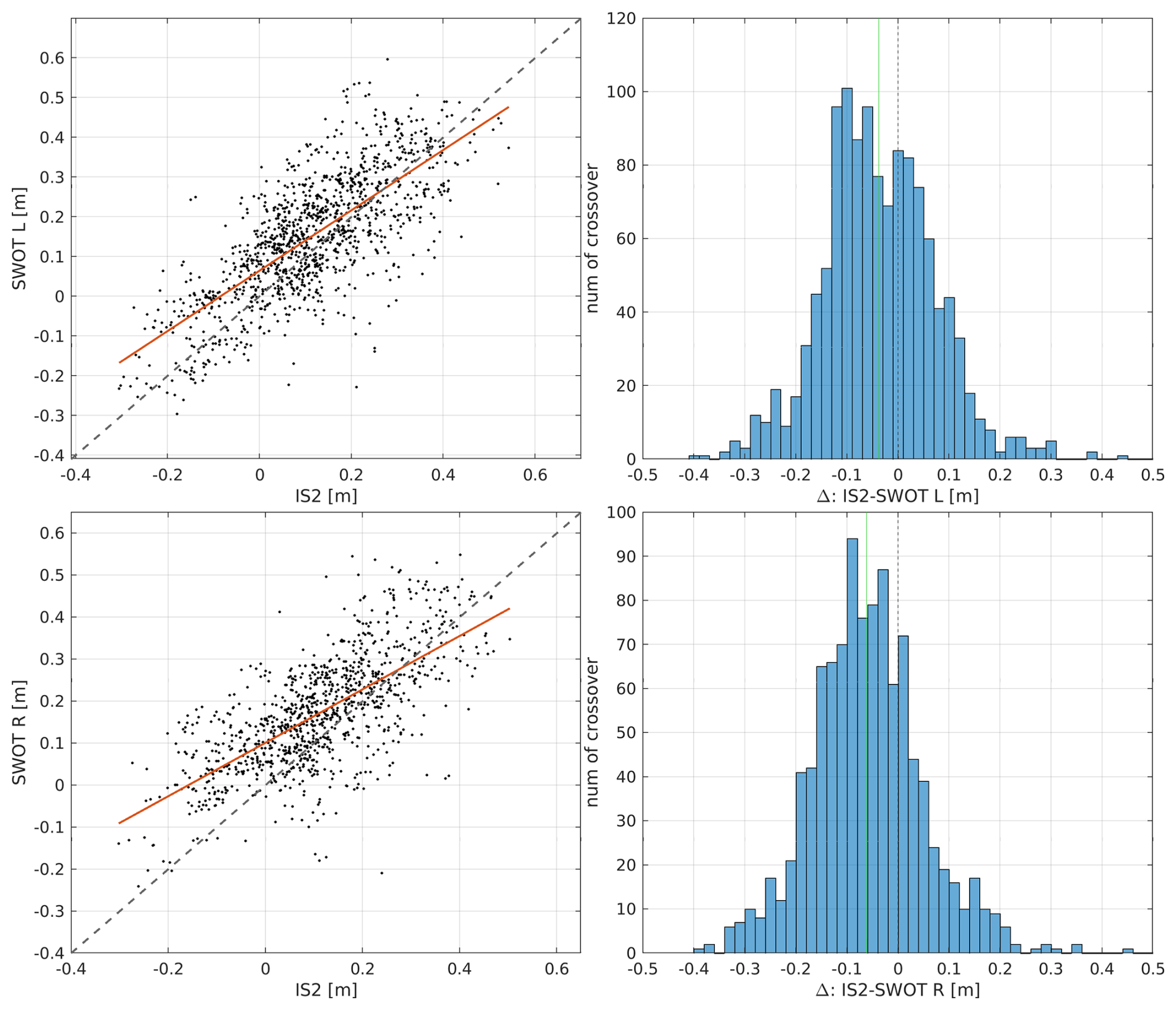
Figure 7 Scatter plot of ICESat-2 surface height against interpolated SWOT surface elevations per crossover for all 3 beams with regression line (red) and bisectrix (dashed) with histograms of mean value differences for left (top row) and right (bottom row) SWOT swaths. In the histograms, the mean values (−4 cm for left and −6 cm for right swath) are indicated by the green line, while the zero line is indicated as a dashed line.

Regarding the mean values of the differences, the two swaths behave quite similar and show discrepancies of −4 cm (left) and −6 cm (right), see histograms, green lines. These discrepancies are not significant given a standard deviation of around 11 cm for both sides. The trend lines indicate that the mean values of SWOT tend to be systematically lower in relation to ICESat-2. SWOT shows a smaller variation in the mean values than ICESat-2, i.e. it is less sensitive to changes in height than ICESat-2.

The spatiotemporal differences between the left and right SWOT swaths are further studied in Fig. 8. It shows the absolute differences, averaged for ICESat-2 overflights, of the mean values between the interpolated SWOT observations for the left and the right swath during the winter months January/February, which are featured by extended sea ice conditions and high crossover availability (see Fig. 9 right). It can be seen that there are generally larger deviations of up to 50 cm in January/February, for example in the Beaufort Sea or northern Laptev Sea. These areas are characterised by sea ice coverage of several months and high sea ice dynamics. During the other months (Fig. 8, right), the deviations are smaller and do not show a clear region-dependency.

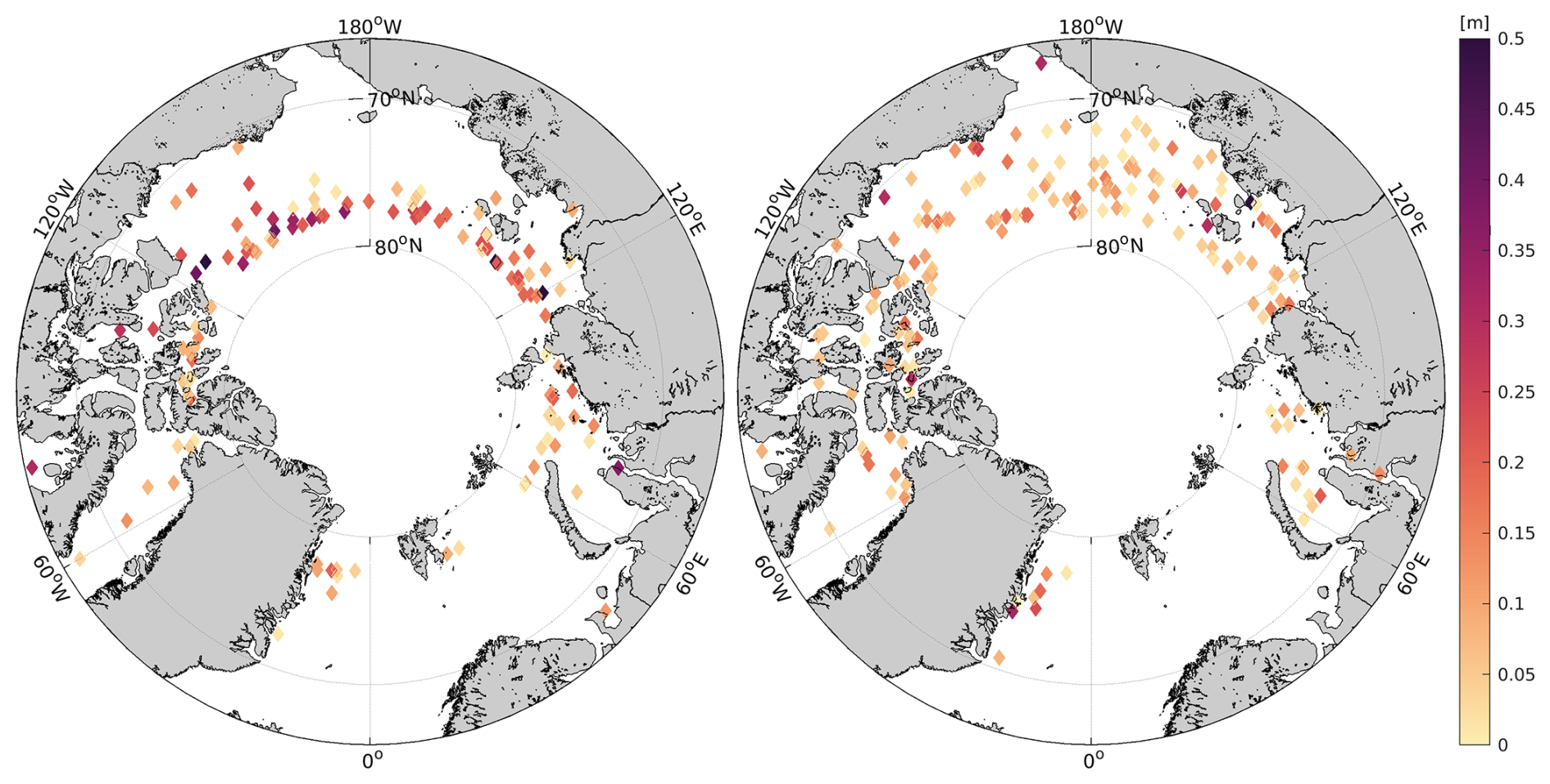
Figure 8 Absolute mean surface elevation differences of the interpolated SWOT observations between the left and right swath for January/February 2024 (left) and other months (right). Different laser beams are averaged per swath side. Only crossovers where the left and right swaths are available and overflown by ICESat-2 are shown.

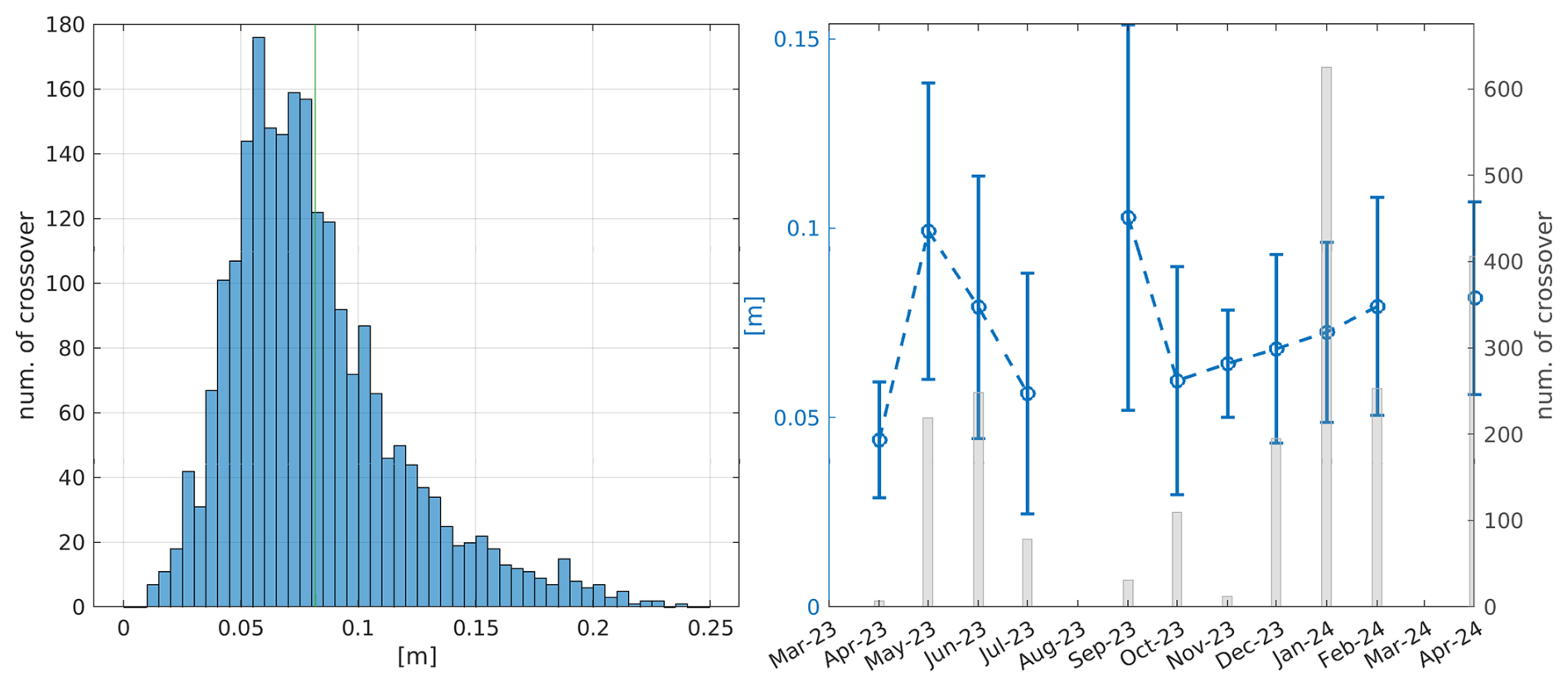
Figure 9 Histogram (left) and monthly averaged evolution (right) of all standard deviations of point-wise surface elevation differences between interpolated SWOT swath values and strong ICESat-2 laser beams. Green line in histogram indicates mean value of 0.08 m

Next, in order to analyse the height differences, the mean values are subtracted from the ICESat-2 laser profiles and the interpolated SWOT observations per swath side. Figure 9 (left) displays the histogram of the standard deviations of these zero-centred differences. The standard deviations scatter around 0.08±0.04 m and are almost normally distributed. Calculated Pearson correlation coefficients show predominantly positive and left-skewed correlations scattering around 0.4 with maximum values up to 0.99. With regard to seasonal variations, the lowest standard deviations are observed in autumn and at the beginning of winter between October and December, while higher standard deviations appear during the melting period from May to June. However, the summer months are characterised by a larger uncertainty range, as fewer crossovers are available due to the required sea ice coverage of at least 15 %.

As shown in Fig. 10, the standard deviations of the crossovers are widely distributed across the Arctic Ocean region covered by SWOT. While in most areas the deviations are in the range of 4–8 cm, there are increased values in the area of the Canadian Archipelago, the Beaufort and Greenland Sea as well as the Northeast Greenland Shelf.

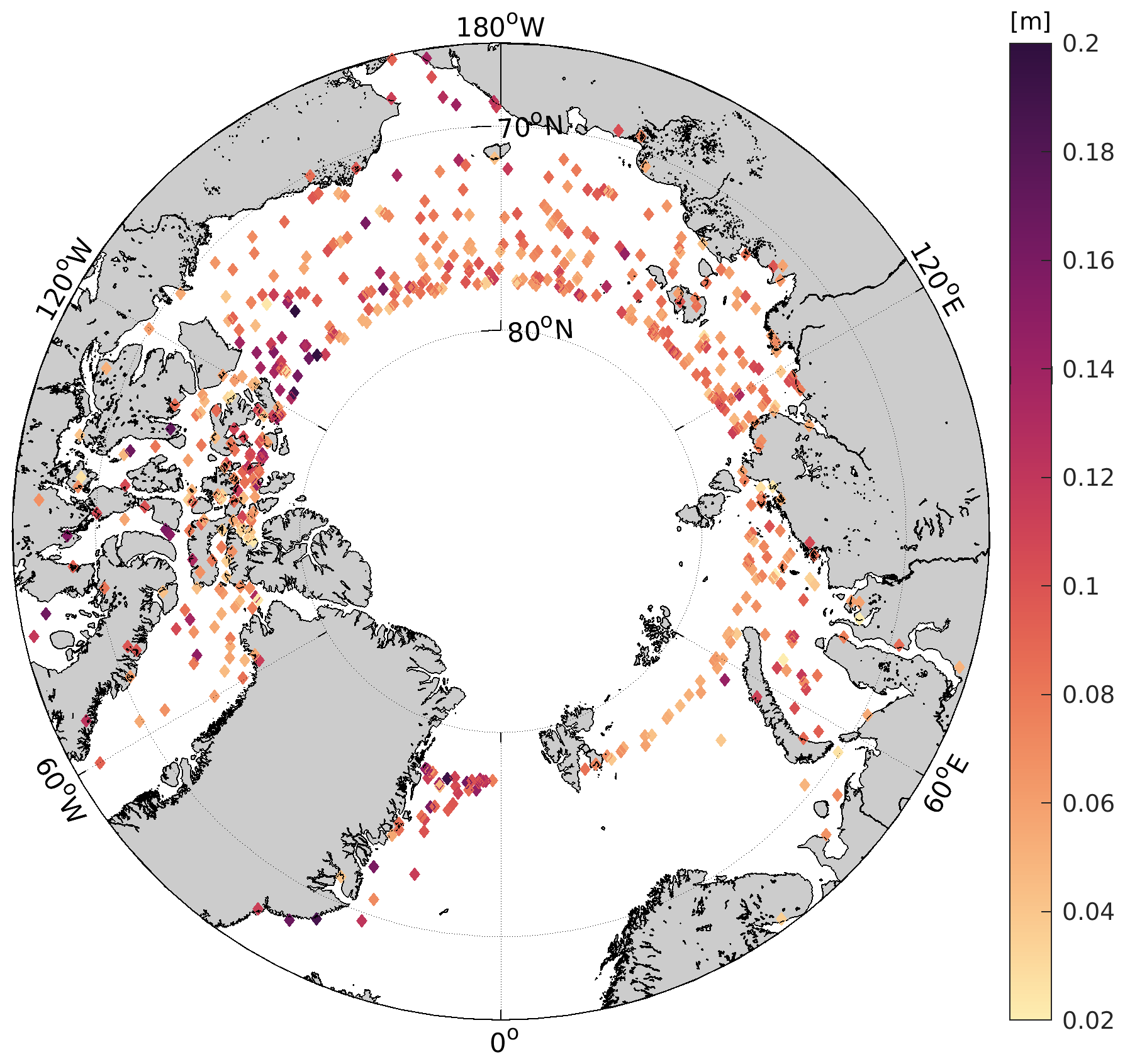
Figure 10 Spatial distribution of standard deviations of point-wise surface elevation differences averaged per crossover (both swath sides and all three laster beams) during the study period from March 2023 until April 2024.

All discussed analyses refer to point-wise comparisons of observations without differentiating between observations of sea ice and open water surfaces. To get an impression of how SWOT behaves in the case of open water spots in sea ice cover, the ICESat-2 ATL07 flag height_segment_ssh_flag (Kwok et al., 2023) is applied and only filtered for open water (i.e., lead) observations detected by the ICESat-2 processing chain. This reduces the number of valid comparison points dramatically to about 180.000 (from 11⁶) and decreases the mean standard deviation to 0.06±0.04 m, while the correlation remains unchanged.

4 Discussion and conclusions

The study presents an initial assessment of SWOT swath heights in the Arctic Ocean by comparing them to ICESat-2 laser altimetry heights and Sentinel-1 images. The SWOT orbit inclination does not enable a full coverage of the Arctic Ocean, but nearly 550 overlaps within a 30 min time frame with ICESat-2 provide the basis for visual and quantitative comparisons. Care was taken to cover as much of the sea ice period in order to observe SSH during different sea ice conditions. The SWOT data used is limited to L2 LR Unsmoothed KaRIn swath observations, as this is the predominant observation mode with the highest spatial resolution of SWOT in the Arctic Ocean. However, meaningful surface heights, including all necessary geophysical corrections, can only be generated with great effort when using the SWOT Version C data by additionally including the L2 LR Expert dataset. The more recent Version D makes this problem largely obsolete, but this version is currently only available for the most recent SWOT observations.

One critical aspect for the reliable SSH determination using SWOT is the application of the so-called height correction from the crossover calibration. During the SWOT pre-processing (Sect. 2.1), bad values of this correction are removed or not used, but since alternatives are missing in the ice-covered oceans, crossover calibration corrections marked as “suspect” (Fig. 1) are still applied. This results in the expectation of erroneous corrections, which can reach up to around 50 cm (Fig. 6) in this study. The reason for these deviations probably lies in the way this correction is calculated for L2, as only crossovers of SWOT-SWOT overflights during open ocean conditions are used and interpolated for the observations in between. In areas of persistent ice cover, such as the northern parts of the Arctic Ocean or the Beaufort Sea and the Laptev Sea, this can very likely lead to large uncertainties. The analysis of the data also clearly reveals that larger areas close to the edge of the SWOT swaths (approx. 5 km on each side) are very noisy and should not be used for scientific analyses.

The assessment demonstrates that SWOT has the potential to provide valuable 2D surface height observations during sea ice conditions. In particular, leads and open water areas, identified by their relative height differences between the sea ice surface and open water patches, are clearly recognizable and respective data agree with ICESat-2 along-track height observations. In addition, SWOT is able to record small-scale elevation variations across the ice-covered surfaces, for example, of larger sea ice areas or bigger ice floes. Compared to SAR images from Sentinel-1, there is a remarkable coherence between the observed swath elevations and the interpolated grey-scaled backscatter values, which allows for conclusions about different sea ice surface types (e.g., leads, ice floes etc.). A quantitative evaluation of the point-wise comparisons provides a mean value of the standard deviations of the differences per laser ground track of 8 cm. The mean standard deviation reduces to 6 cm when only open water points are considered. For this comparision the ICESat-2 lead flagging is used, directly taken from the ATL07 product (Kwok et al., 2023).

With respect to small-scale features of the ice-covered sea surface, surface elevations from SWOT appear smoother and are characterised by more gradual transitions between the sea ice edges and open water. In contrast, ICESat-2 profiles tend to show more pronounced elevation variations and a clearer separation of different height or sea ice features (even if filtered to the sparser SWOT resolution). This indicates that the SWOT LR dataset can resolve small open water and sea ice areas only to a limited extent. Besides wavelength differences, this can also be attributed to the different sample resolutions. Kacimi et al. (2025) also reported that it is difficult for SWOT LR data to capture surface features at shorter length scales. Higher-resolution data sets of SWOT (e.g. HR, pixel-cloud) could likely reduce this discrepancy. However, besides the resolution, other factors contribute as well. One might be the different snow penetration of both instruments.

It is common knowledge that the ICESat-2 laser data hardly show any penetration into snow or ice and represent the entire sea ice surface height (i.e. freeboard), including a possible snow layer (Petty et al., 2023). In contrast, it is still unclear how KaRIn-derived elevations are affected by varying surface conditions, for example by snow load or thin ice. In this context, there is a lack of knowledge about the sensitivity of KaRIn to different snow and sea ice properties under the influence of off-nadir incidence angles, which affect the signal propagation and backscattering behaviour. In general, K_a-band penetrates less deeply into the snow than the K_u-band and tends to reflect at the upper portion of the air-snow interface (e.g. Willatt et al., 2025, Fredensborg Hansen et al., 2025, Guerreiro et al., 2016). According to first investigations, this penetration behaviour is also to be expected for KaRIn (Jutila and Haas, 2025, Fayne et al., 2024). But, in order to gain deeper insights into KaRIn's signal propagation, detailed studies based on in-situ or airborne validation data are required (Armitage and Kwok, 2021).

Besides the reasons on the side of instruments and data processing, it should be mentioned that the discrepancies of the acquisition times of the satellites add additional uncertainties due to sea ice dynamics or environmental changes, such as strong drifts, which can reach monthly drift velocities ranging from 280±112 m h⁻¹ in April 2024 until 415±154 m h⁻¹ in January 2024 on average. Dependent on the season, the highest drift velocities occur in the Beaufort Sea, the Fram Strait, and the East-Greenland Current region (OSI SAF and EUMETSAT SAF On Ocean And Sea Ice, 2010). Additionally, steep temperature gradients can cause rapid openings and closings of leads.

The 30 min limit applied provides a good compromise, but a gap of 60 min as shown in Fig. 4 between the SAR image and altimetry more likely leads to displacements. Further challenges arise in the occurrence of roughed water surfaces, e.g., during strong-wind conditions or the presence of frost flowers, as this leads to uncertain surface heights in the swath data. This underlines the need for further investigations of KaRIns' backscattering characteristics and the height determination during such conditions.

Despite these uncertainties, significant new findings can be expected from SWOT in sea-ice-covered oceans. Its swath data is a great innovation in the determination of polar sea level under the influence of sea ice and rapidly changing surface conditions. For the first time, spatial, 2D height information for sea ice thickness or freeboard determination can be provided. We should try to learn as much as possible from the SWOT mission in order to pave the way for the future S3NG-T mission, which includes the cryosphere as a secondary objective and will extend the monitored area to a geographical latitude of 81.5° N.

However, the study also shows that there is room for improvement in the SWOT data for generation of sea surface elevation data under sea ice conditions. On the one hand, this concerns SWOT-dedicated corrections adapted to sea ice conditions, but also to reliably distinguish open water from sea ice. Since currently no SWOT observation-based sea ice surface classification exists, special focus must be given to the development of a robust classification method to detect leads. This requires a better and deeper understanding of the K_a-band backscattering behaviour of KaRIn under different conditions at the sea surface during the presence of sea ice. In this context, it is crucial to integrate information from in-situ or airborne campaigns and K_a-band (i.e. SARAL) as well as laser altimetry. For example, the more detailed lead (e.g. dark/specular leads) type determination of ICESat-2, available in ATL07, can provide further information on different lead types (e.g. dark, bright) and the evaluation of SWOT-derived SSH within leads.