Bias-adjusted projections of snow cover over eastern Canada using an ensemble of regional climate models

In the context of climate change, stakeholders and decision makers need easily accessible bias-adjusted projections of snow cover and indices produced from those to develop adaptation plans. To meet this need, we produced an ensemble of statistically bias-adjusted regional climate projections of snow water equivalent (SWE) in the province of Québec, Canada. This bias adjustment required some fine-tuning to operational methods, mainly due to the seasonality in the SWE. We calculated indices of interest for several sectors based on the bias-adjusted SWE. These indices included the maximum of SWE as well as the duration, start, and end of the snow season, and the days without snow cover. In eastern Canada, snow cover tends to persist for shorter periods as the climate warms, with symmetrical shrinkage at the beginning and the end of the snow season, with the exception of the Nunavik region. The maximum SWE is projected to decrease in the southern part of the domain and increase elsewhere. The snow season in the Côte-Nord, southern Québec and St-Lawrence River Valley regions is increasingly interrupted by sequences of days without snow cover, whereas this is not the case for the northern and central Québec regions.

1 Introduction

Changes in snow cover have significant feedback on climate (Déry and Brown, 2007; Flanner et al., 2011). The Northern Hemisphere witnesses a decrease in snow cover extent, a shortening of the snow season (Derksen et al., 2019; Mudryk et al., 2020; Fox-Kemper et al., 2021; McCrary et al., 2022) and a greater warming than in the rest of the world for the Arctic part (e.g. Hoegh-Guldberg et al., 2018). These changes in snow cover affect water supply (e.g. Mankin et al., 2015), agriculture (e.g. Bélanger et al., 2002), ecology (e.g. Zimova et al., 2016), hydroelectricity or flooding through streamflow changes (e.g. Dudley et al., 2017; Arora et al., 2025), tourism (e.g. Scott et al., 2020) and more. Stakeholders and decision makers need accurate climate information to adapt to climate change (IPCC, 2022). The widespread practice in climate services is to adjust the bias of global climate simulations and combine them in an ensemble to provide ensemble statistics (Lavoie et al., 2024). Impact models can be sensitive to small systematic biases that are present in the global climate models (GCMs) or inherited by regional climate models (RCMs) from their driver (Maraun et al., 2010; Muerth et al., 2013). Bias adjustment helps reduce these biases, which also reduces the inter-model differences and eases their combination into multi-model ensembles. Currently, this is only applied to a subset of variables for which statistical adjustment has been more extensively studied, namely near-surface temperature (2-m temperature) and precipitation and mainly on GCM simulations (e.g. https://portraits.ouranos.ca, last access: 12 December 2025, Climate Portraits, https://climatedata.ca/, last access: 12 December 2025, https://atlas.climate.copernicus.eu/atlas, last access: 12 December 2025, Climate Atlas of Copernicus). Several climate indices are derived from these bias-adjusted variables. Extending the production of bias adjusted variables can be challenging. Some variables such as freezing rain have rare occurrences. Other variables such as snow on the ground or precipitation in regions with a monsoon regime exhibit strong seasonality. These features are difficult to handle with standard bias adjustment techniques, which often rely on quantile mapping. Declined in multiple variants (see  Gutiérrez et al., 2019 for an exhaustive list), these methods generally divide the reference and the source into quantile-based bins and for each bin, find an adjustment factor that is applied either additively or multiplicatively, depending on the adjusted variable. Particularly, it is the zero-bounded aspect of surface snow that makes it more difficult as additive correction can create nonsensical negative values and multiplicative correction is incapable of adjusting values that are zero in the source.

The snow cover variables such as snow depth or snow water equivalent are simulated by land surface models (LSMs), such as Crocus (Brun et al., 2013), CLASS/CLASSIC (Verseghy, 1991; Melton et al., 2020), or HTESSEL (Dutra et al., 2009). Each LSM has its pros and cons (e.g. Lee et al., 2024). The LSMs can be used coupled with the atmosphere in a GCM or RCM, like CLASS in the Canadian Regional Climate Model version 5 (CRCM5;  Martynov et al., 2013; Šeparović et al., 2013). Users can then work with the snow data produced by a climate model coupled to a LSM and such data are already available through projects like CMIP6. This option has drawbacks, as the raw models have a coarse resolution (200 km and more for GCMs, 10 to 50 km for RCMs) and their biases in temperature and precipitation for example have not been addressed. LSMs can also be used in an offline-mode, which presents some advantages, like allowing a higher resolution to have more accurate orography. For example, ERA5-Land (Muñoz-Sabater et al., 2021) is run off-line, forced by ERA5 atmospheric fields (Hersbach et al., 2020), has a finer resolution (9 km) than ERA5 (0.25°), uses a daily environmental lapse rate to adjust air temperature for the altitude differences, and has an overall better performance than ERA5 for snow water equivalent (SWE). As bias adjustment of temperature and precipitation is better understood, it can also be performed on the drivers (GCMs or RCMs) of such offline LSMs (Luca et al., 2017; Morin et al., 2021). Using bias-adjusted inputs in offline LSMs adds a step in the simulation of snow at a high resolution. However, no feedback between the surface and the atmosphere are allowed when LSMs are used offline.

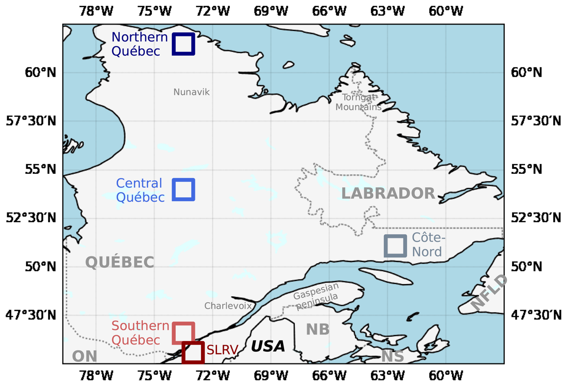
Figure 1 Studied domain. Boxes outline the following regions: northern Québec (dark blue), central Québec (blue), Côte-Nord (gray), southern Québec (light red) and St-Lawrence River Valley (SLRV; brown). NB: New Brunswick; NFDL: Newfoundland; NS: Nova Scotia; ON: Ontario.

To the best of our knowledge, these are the two possibilities to work with snow depth or SWE projections (LSM coupled to a GCM or RCM, and LSM in offline-mode). On the other hand, different users need accurate climate information with a high resolution in a large domain. To fill the gap between supply and demand, we propose to generate and give access to an ensemble of bias-adjusted snow cover indicators based on snow data produced by RCMs with an horizontal resolution of 0.1°. This will make use of the RCMs' advantages: finer resolution than GCMs, coupled LSM, large domain for wide applicability. Moreover, this method remains easy to operationalize, as no LSMs needs to be run offline. In terms of bias adjustment methods, some have been applied to snowpack characteristics (Matiu and Hanzer, 2022), but these methods were exclusively considered for the snow cover fraction. To our knowledge, there is only one bias adjustment method that has been successfully applied to the snow amount, or snow water equivalent (SWE; Michel et al., 2024). We will use the re-insertion of non-zero SWE values near the snow end season as proposed in Michel et al. (2024) before applying empirical quantile mapping to bias-adjust the SWE data. Furthermore, snow cover indices will be computed based on the bias-adjusted SWE. The choice of the variable (SWE instead of snow depth) allows us to focus on the total water content in the snowpack, which, contrary to snow depth, is independent of the snow density. We produced the SWE indices for a domain including the Canadian province of Québec (eastern Canada). This domain has mountains of medium altitude, which alleviates problems often arising with snow simulation in high-altitude terrain (orographic forcing missed due to coarse resolution and smoothed orography) such as the Rocky Mountains (e.g. Santolaria-Otín and Zolina, 2020; Kouki et al., 2022; McCrary et al., 2022).

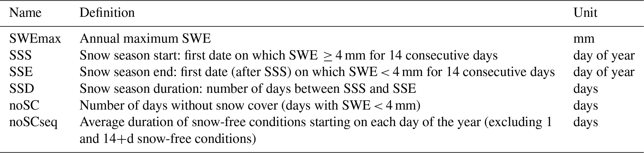
Table 1 List of snow cover indices characteristics (name, definition, unit).

This article is organized as follows. Section 2 presents the data, methods and domains used to produce the snow cover indices ensemble, which is then analyzed in Sect. 3. Discussion follows in Sect. 4 before a conclusion in Sect. 5.

2 Data and Methods

2.1 Domain and regions of interest

The study domain encompassed the Canadian province of Québec and included New Brunswick and parts of Labrador, Newfoundland, Ontario, Nova Scotia and northeastern United States (Fig. 1). Five smaller regions (10 × 10 grid points, that is, 1° × 1°) were defined to present a climatic diversity (Fig. 1). The southern, central and northern Québec domains followed a North-South transect along the same longitude to investigate the meridional gradient. These regions have the same range of altitude, with respectively, in average, 468, 391 and 356 m. The effect of an altitude gradient was studied by comparing the plains in the St-Lawrence River Valley (SLRV) with southern Québec, as these domains share a similar latitude range but different mean altitudes (respectively 59 and 356 m). Comparison between a domain with more oceanic influence (Côte-Nord; 390 m altitude) and a continental domain (central Québec) was also considered. These domains are represented by coloured boxes in Fig. 1: northern Québec (dark blue), central Québec (blue), Côte-Nord (gray), southern Québec (light red) and St-Lawrence River Valley (SLRV; brown). Results presented for these regions correspond to the spatial mean within the area.

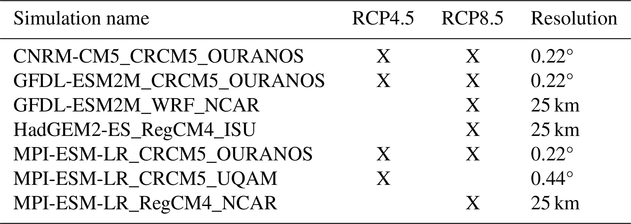
Table 2 Ensemble of simulations considered in this paper. Simulation names correspond to Driving-GCM_RCM_RCM-Institution. More details can be found in the Supplement.

2.2 Snow cover indices

Several indices were studied to describe the behaviour of the snow cover: Start (SSS), End (SSE) and Duration (SSD) of the snow season; Annual maximum SWE (SWEmax); Days without snow cover (noSC). Their characteristics are specified in Table 1. Snow cover was defined as a SWE ≥ 4 mm (Mudryk et al., 2017), consequently noSC was defined as days with SWE < 4 mm. SSS was the first day of the first 14 consecutive days with snow cover, and SSE was the first day, after SSS, without snow cover for 14 consecutive days. The snow season duration was simply the number of days between those dates. Note that the snow season can include days without snow cover, as long the 14 d streak is not reached. The 14 d threshold was chosen for two reasons: it was long enough to avoid an artificially short snow season when the snow cover is often interrupted by brief warm spells, and it was short enough to be of use for stakeholders and adaptation planners, in opposition to a 30-d threshold like the one used in Brown (2010). Indeed, with a 30-d threshold for example, some regions in southern Québec could have no snow season at all due to the fragmentation of the snow cover by the end of the century. Considering more than two weeks for the SSS and SSE triggers can also limit the use of such indices for adaptation plan. Indices are calculated annually for winter years, starting on 1 August and ending on 31 July on statistically bias-adjusted SWE time series from an ensemble of RCM simulations described in the next section.

For analysis purposes, another indicator, noSCseq, was defined in order to investigate the fragmentation of the snow cover. noSCseq looks at sequences of 2 to 13 consecutive days without snow cover (days with SWE < 4 mm). We chose a limit of 13 consecutive days for noSCseq in order to consider only the period during which a snow season could be present, since our threshold for the SSS [SSE] is 14 consecutive days with [without] snow on the ground (Table 1). We found all such sequences for all regions and for each periods of 30 years. We grouped these by the day of year on which they start and took the 30 years mean of their length, which enabled us to obtain climatological data on the duration of noSCseq starting on each day of the year in each region for different horizons. Finally, as described in Sect. 2.1, spatial mean within the area was performed for each region.

2.3 Data

2.3.1 Reference data

For this study, the historical period (1991–2020) was defined as 1 August 1991 to 31 July 2021. We considered reference data that provided daily SWE data on a high-resolution grid with a coverage of the historical period. For the Québec province, several SWE gridded databases like ERA5, ERA5-Land, MERRA-2 or B-TIM products are available (Molod et al., 2015; Mudryk et al., 2015, 2017, 2025; Hersbach et al., 2020; Muñoz-Sabater et al., 2021; Elias Chereque et al., 2024; Mortimer et al., 2024). However, spatial differences were observed between such databases (Mudryk et al., 2015, 2025). Studying the Northern Hemisphere, Mudryk et al. (2015) highlighted that the spread in climatological values was mainly due to the different land surface models simulating the snow water mass in the reanalysis products.

ERA5-land has been used as the reference dataset in many climate services applications at Ouranos at the time of the project and Mudryk et al. (2025) showed that it has a good SWE performance for eastern North America among other products. This led us to consider ERA5-Land as reference product in this study. ERA5-Land was produced by a land surface model (HTESSEL) running offline, driven by ERA5 atmospheric fields and without SWE observations assimilation. ERA5-Land has a 0.1° horizontal resolution and an hourly temporal resolution, and its SWE data is publicly available (named “snow depth water equivalent”). ERA5-Land has some biases. Leduc and Logan (2025) highlighted that the warm bias of daily minimum near-surface temperatures in ERA5-Land induces a bias in the climatology of the freeze-thaw events, which they define as a day when the minimum temperature is below 0 °C and maximum temperature is above 0 °C and such a bias could also have an effect on the SWE. Kanda and Fletcher (2025) analyzed the bias of ERA5-Land SWE across Canada against Canadian Historical Snow Water Equivalent observations (CanSWE; Vionnet et al., 2021), for three ranges of elevation. In Québec, the selected stations belonged in either low or medium elevation categories. In their results, they highlighted that ERA5-Land tends to underestimate large snow-packs (exceeding 300 mm, mainly high-altitude stations), well-estimate mid-elevation regions, and underestimate low-elevation regions. For a more local overview of ERA5-Land performance, an analysis was performed to assess ERA5-Land against observations from CanSWE and GovQC (Ministère de l’Environnement, de la Lutte contre les changements climatiques, de la Faune et des Parcs, 2020) datasets on our studied domain (see Sect. 3.1).

2.3.2 RCM Simulations Ensemble

The list of mandatory archived variables for the Coordinated Regional Climate Downscaling Experiment (CORDEX; Giorgi et al., 2009) did not include SWE. Only certain modelling institutions archived and shared their SWE data. This led to a preliminary simulation ensemble encompassing only a subset of the simulations produced through the North America CORDEX (NA-CORDEX,  Mearns et al., 2017) project, to which several additional simulations from the CRCM5 (Martynov et al., 2013; Šeparović et al., 2013) ran at Ouranos were added, leading to a first ensemble of 26 simulations (9 with RCP4.5 and 17 with RCP8.5; Table S1 in the Supplement).

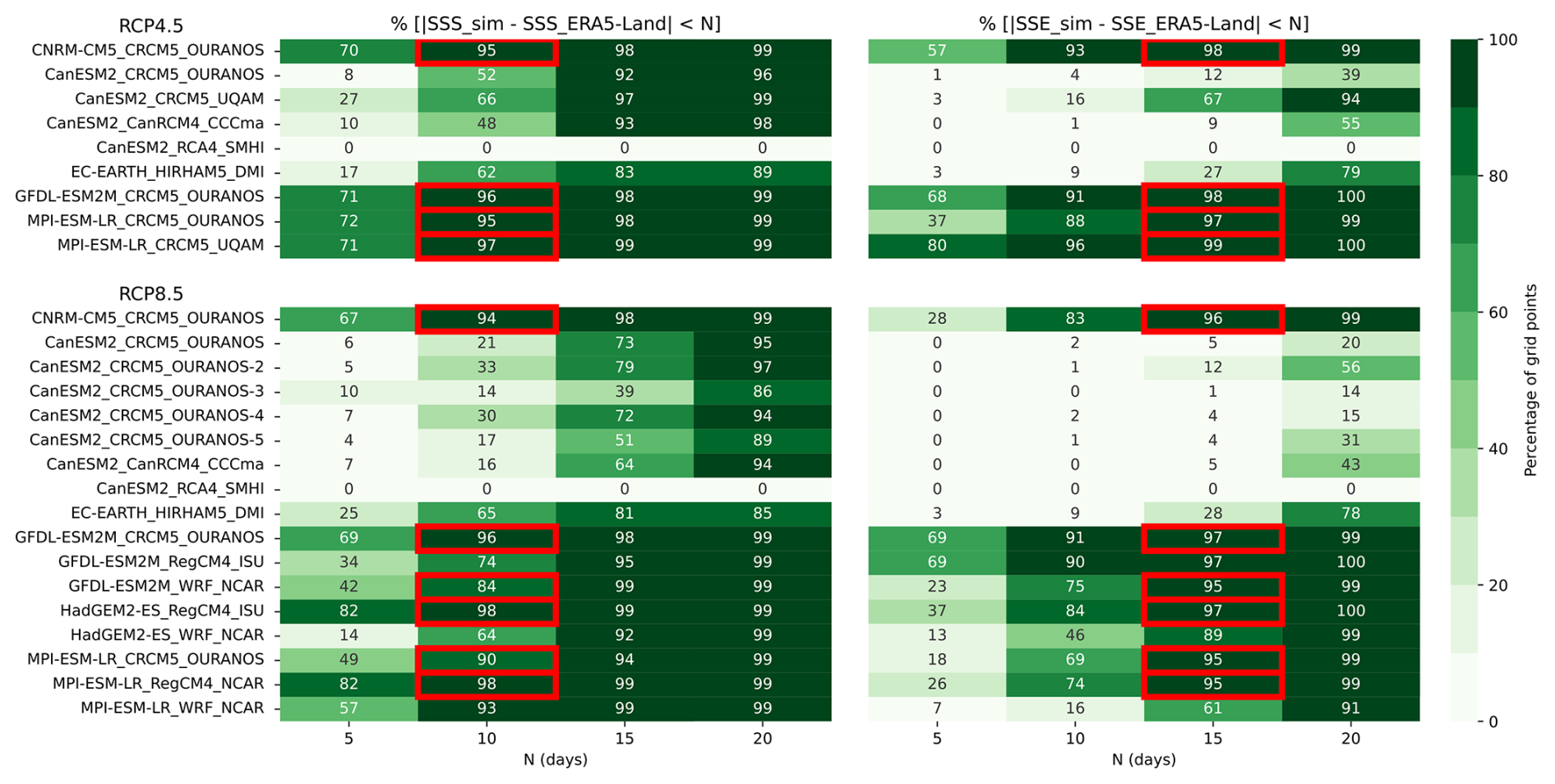
Figure 2 Percentage of grid points with a SSS bias (left) within a ± N days interval and a SSE bias (right) within a ± N days interval, below the 50° N for all RCP4.5 (top) and RCP8.5 (bottom) simulations. Red boxes present values for the selected simulations. Simulations names correspond to Driving-GCM_RCM_RCM-Institution.

A first inspection of the simulated SWE from RCMs showed large discrepancies between simulations (Figs. S1 and S2), as already highlighted in the literature (e.g. McCrary et al., 2017), forcing a selection of simulations to build the ensemble. Indeed, to perform a statistical bias adjustment on a variable with a strong annual cycle like SWE, a good synchronization in the timing of the melting and accumulation periods is needed. Specifically, a simulation with a short snow seasons bias posed challenges, as the longer sequences without snow cover could have not been adjusted with usual multiplicative methods. Common statistical bias adjustment methods do not adjust the seasonality of variables explicitly and will not perform well for a variable that is exactly zero for long stretches of time, such as SWE.

A selection of simulations was thus required, and this was a limitation for the bias-adjustment method that was prioritized. This procedure balanced selecting the best-performing simulations with maintaining an ensemble large enough to capture uncertainties across emission scenarios and RCMs. The selection criteria were based on the SSS and SSE indices described above, and focused on the southern part of the domain (< 50° N). This region was chosen because it is the most densely populated and most of the requests for adaptation about snow cover indices came from this region. Moreover, more observation stations are available in this region leading to more observation assimilation in the reanalysis ERA5, which is used as input in ERA5-Land. A simulation was kept if, for more than 80 % of the target grid-points, the SSS bias did not exceed 10 d and SSE bias did not exceed 15 d (Fig. 2). Different thresholds were tested. The selected thresholds allow to consider different driving GCMs, RCPs and RCMs combinations to cover uncertainties. The final ensemble included 10 simulations (Table 2) and was compared with results from McCrary et al. (2022) to ensure that no specific problems had been detected in our study area in their work. In their study, they rejected simulations from the RegCM4 RCM as it did not perform well enough mainly in western North America, and also on the southern Baffin Island (unbounded snow accumulations). Our region of interest was not affected by this poor performance and a simulation produced with the RegCM4 RCM was considered, as it met the previous criteria. Hereafter, when results are presented (Sect. 3) for RCP ensembles, it refers to the median of the simulations for a specific RCP.

The selection criteria leads to the rejection of all regional simulations driven by CanESM2, regardless of the member (Fig. 2). This can be related to the warm bias of the CanESM2 model in eastern Canada. This bias leads to less snowfall and more ablation of the snow cover. In Sheffield et al. (2013), the near-surface temperature bias for CanESM2 is presented for the eastern North-America (ENA) domain as described in Giorgi and Francisco (2000). This domain is similar to the domain considered here for the simulation selection with an extension to the South, and the same northern border (i.e. 50° N). For that domain, the aforementioned study shows that CanESM2 has large warm biases for near-surface temperature, regardless of the season, compared to observations for the 1979–2005 period (ENA: 4.79 °C in winter and of 3.4 °C in summer). Sheffield et al. (2013) also show the near-surface temperature biases for GFDL-ESM2M and HadGEM2-ES, and for another domain, Northeast Canada (NEC), which covers the northern part of the province of Québec. There, CanESM2 has a near-surface temperature bias of 3.13 °C in winter and 3.17 °C in summer. GFDL-ESM2M and HadGEM2-ES have greater biases in the NEC domain for near-surface winter temperatures (respectively 5.75 and −5.12 °C) than in the ENA domain (1.35 and −1.61 °C). Such differences in the near-surface temperature biases highlight the fact that the extent of the selection domain has to be carefully chosen and can be a limitation of the present study. Moreover, a more detailed analysis of the reason why the simulations of this ensemble better performs regarding the rejected ones could be of interest but was not the scope of this study.

2.4 Statistical Downscaling and Bias-adjustment Method

The statistical downscaling of the simulations towards the resolution of the ERA5-Land reference is done in conjunction with the bias-adjustment, similarly to Lavoie et al. (2024): In a first step, the simulation cells were interpolated on the ERA5-Land grid using the bilinear method. In a second step, a bias-adjustment procedure is performed on each grid cell separately to correct the bias between the regridded simulations and ERA5-Land. This is similar to the Bias-Correction and Spatial Disaggregation approach (Wood et al., 2002, 2004), with the important difference that the spatial interpolation precedes the bias adjustment which is performed on the finer grid. The period 1991–2020 was used for the training. Both the simulations and the ERA5-Land dataset were resampled to a daily frequency by taking the mean of sub-daily data. The quantile-based approach used for the bias-adjustment is described in what follows.

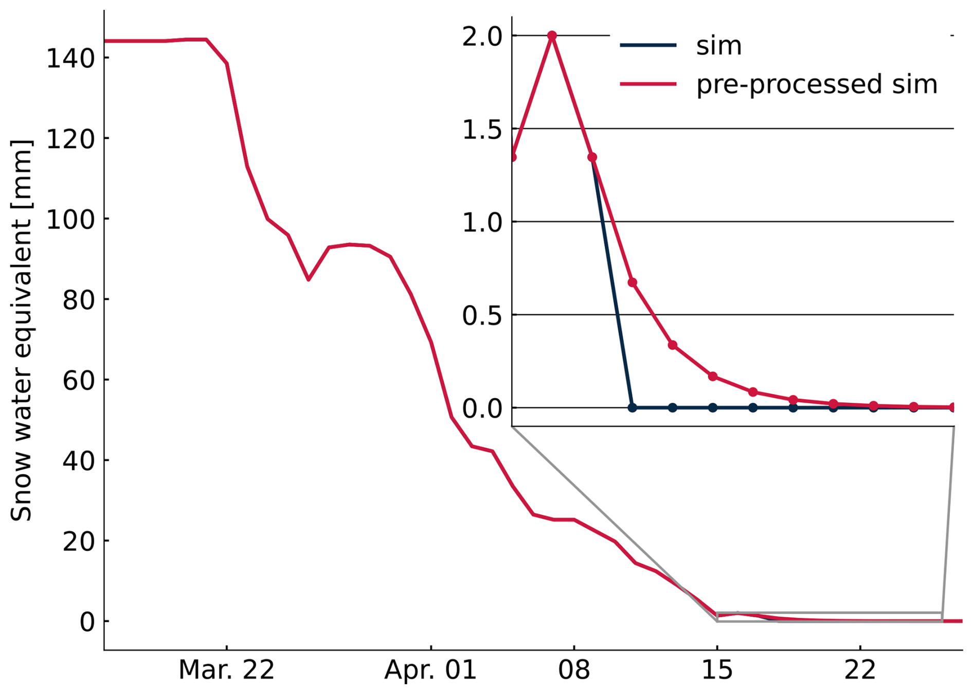
Figure 3 An example of the impact of the pre-processing on a simulation time series at the end of a season for a specific year. A sudden decay of SWE in the original simulation (sim) is smoothened with an exponential decay (pre-processed sim).

SWE time series were adjusted with the Empirical Quantile Mapping (EQM; Panofsky and Brier, 1968; Cannon et al., 2015). We used 48 quantiles, ranging from 0.05 to 0.99 with a 0.02 increment, with the stricter bound in the low tail chosen to ensure a better stability of the bias-adjustment procedure. Temporal grouping was performed for each day-of-year with a 15-d rolling window. We opted for EQM for the following reason: As snow seasons are expected to shorten in a warmer climate, the lower tail of the SWE distribution can become increasingly populated by near-zero values in certain periods of the year. That is, a given quantile in the training period that corresponds to a substantial SWE amount can be associated to a near-zero value in the future. When using EQM, the value in the future is adjusted as near-zero values in the past. On the other hand, a method like Quantile Delta Mapping (QDM) will apply the same correction that was applied to the substantial SWE amount in the past. In other words, the EQM method is less sensitive to a regime change from a period with snow-domination to a period with snow-scarcity.

Statistical methods based on the adjustment of marginals can be limited in their ability to correct SWE time series. Since SWE is a variable bounded by 0 (a ratio variable), it is common to use multiplicative adjustment factors for each quantile when using quantile-mapping-based methods. This guarantees that SWE remains positive. However, if a simulation is biased and, for example, the SSE (i.e., when the snow cover has completely melted) is too early in the year, then multiplying 0 by an adjustment factor will not correct the lack of snow.

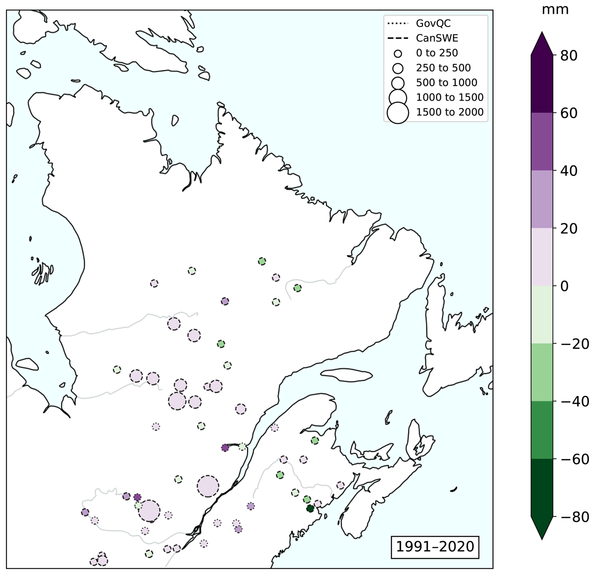
Figure 4 Median bias (mm) for ERA5-Land against observations for the reference period 1991–2020. The size of the symbol represents the number of available observations per station; colour indicates bias magnitude. CanSWE and GovQC stations have dashed and dotted contours, respectively. © Gouvernement du Québec, Ministère de l'Environnement, de la Lutte contre les changements climatiques, de la Faune et des Parcs, 2020.

A similar phenomenon can occur for precipitation, when the source distribution has a higher frequency of dry days than its target. In this instance, small values of precipitation can be randomly distributed throughout the source time series to address this issue and help with the adjustment (Themeßl et al., 2012). In the case of SWE, the problematic values occur in consecutive days of the year. Changing a large fraction of these zeros is then more delicate, as it would effectively prescribe a synchronous adjustment of the time series. In the case of precipitation just mentioned, the pre-processing is rather statistical in nature, and simply precedes more statistical adjustments.

To address these issues, we adapted the pre-processing method proposed in Michel et al. (2024) that precedes the EQM adjustment of the SWE time series. This method specifically aims to improve bias adjustment during the end of snow seasons where the melting mechanism is at play. The idea is to artificially extend the melting period by replacing vanishing values of SWE with small non-zero values. These small values can then be adjusted with a multiplicative factor computed from the ratio of reference over the biased simulation values. When snow season ends occurs too early in a biased simulation, the algorithm inflates the small values in the original simulation (sim in Fig. 4) to make them more similar to the reference (here ERA5-Land). In the opposite situation where the snow season end occurs too late, then adjustment factors of 0 are applied, returning those added non-zero values to 0.

This pre-processing is implemented by modelling the extended melting period with an exponential decay, as in Michel et al. (2024). The end of a snow season is mainly controlled by the melting mechanism, which is safer to extrapolate than the snowfall responsible for the start of the season. We first define a threshold of 0.001 mm below which SWE values are set to 0. Starting from first zero in a given season of this transformed series, the vanishing values are iteratively replaced by the preceding value divided by two. Once the proposed replacement falls below the threshold 0.001 mm, we stop the decay and keep the remaining zero values as-is. An example of this pre-processing is shown in Fig. 3.

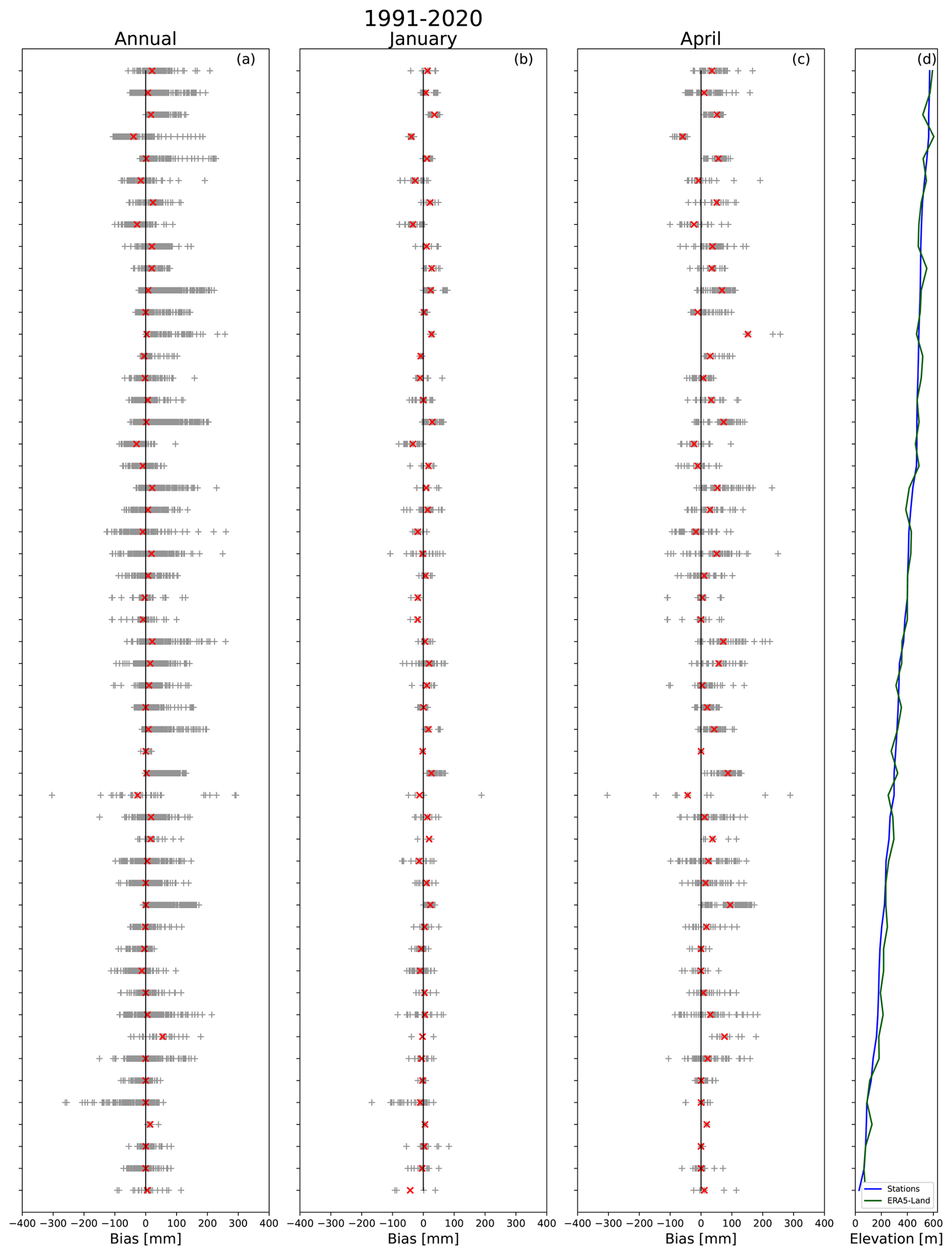
Figure 5 Daily bias (gray crosses) and median bias (red crosses) per station for the whole 1991–2020 period (a), for January (b) and April (c) months in the 1991–2020 period. Only the stations with observations during January and April are shown. Station’s (blue) and ERA5-Land closest grid point’s (green) elevation (d). © Gouvernement du Québec, Ministère de l’Environnement, de la Lutte contre les changements climatiques, de la Faune et des Parcs, 2020.

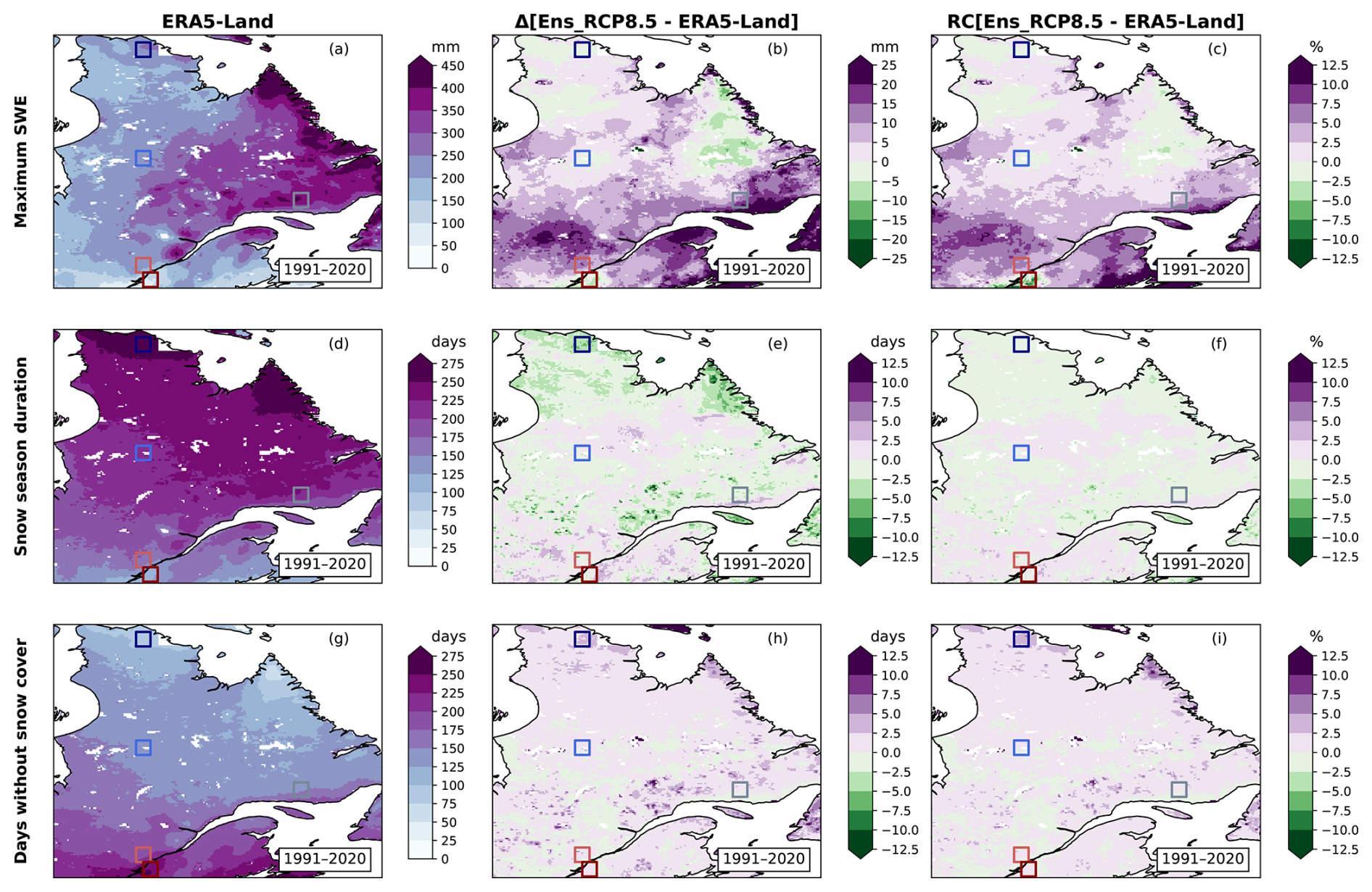
Figure 6 Annual maximum SWE (a, b, c), snow season duration (d, e, f) and days without snow cover (g, h, i) for ERA5-Land (a, d, g), difference (b, e, h) and relative change (c, f, i) between the RCP8.5 ensemble and ERA5-Land for the 1991–2020 period.

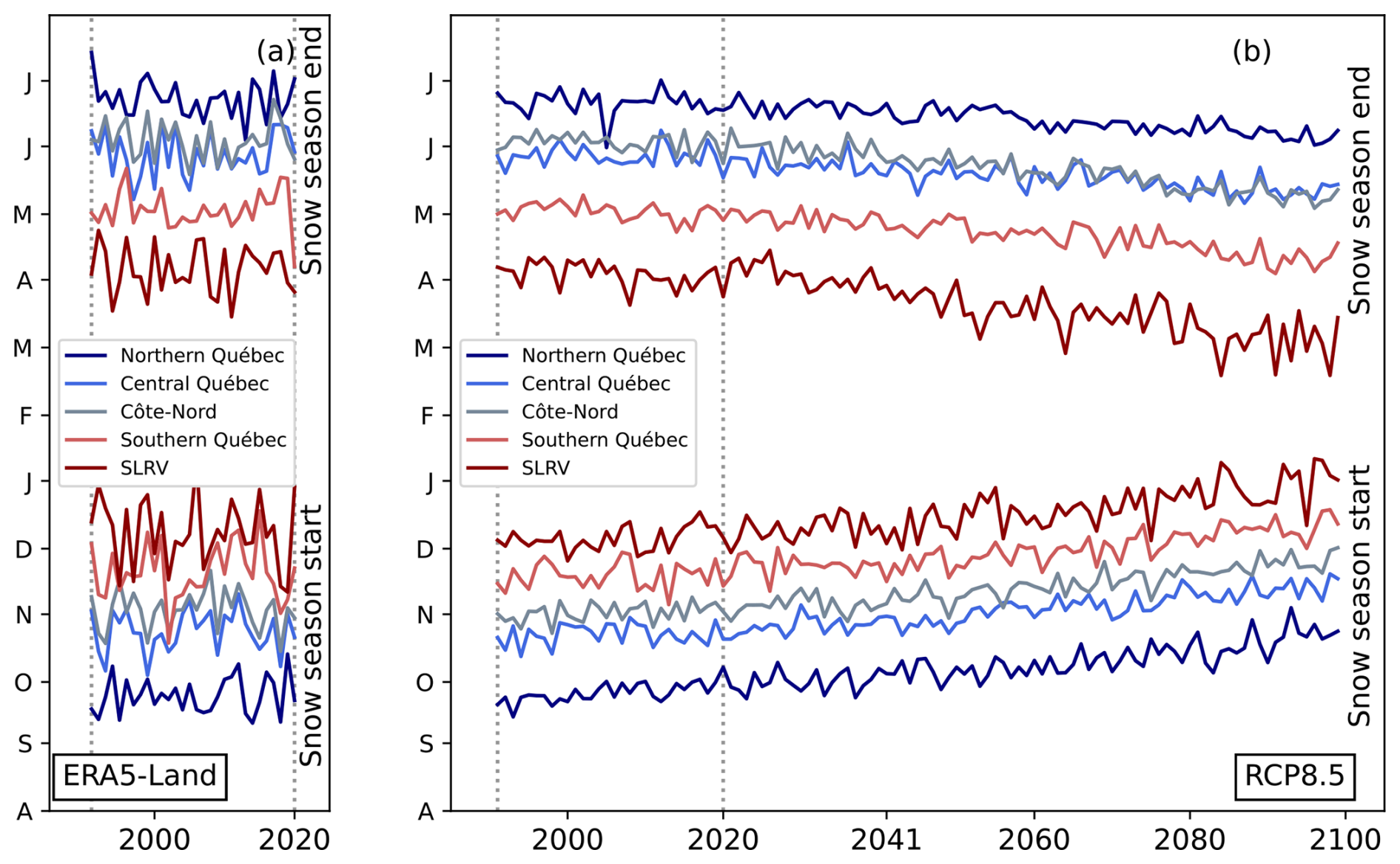
Figure 7 Time series of snow season start (bottom) and snow season end (top) for ERA5-Land (a) and the RCP8.5 ensemble (b) for the five regions of interest. Dashed gray vertical lines encompass the historical period (1991–2020).

Compared to the 0.5 mm threshold proposed in Michel et al. (2024), we use a smaller threshold 0.001 mm to increase the number non-zero SWE data reinserted by the decay process. On the other hand, we restrict the reinsertion of data points near the snow season end, defined as the start of 14 consecutive days below 1 mm threshold for this purpose. Hence, abnormal negligible snowfalls later in the year are not modified with new decaying values of SWE. The smaller threshold 1 mm instead of the 4 mm used for snow season indicators was chosen to apply a stronger filter on abnormal snowfalls.

Following this pre-processing, we applied a frequency adaptation following a standard methodology applied in the context of precipitation adjustment, as discussed above (Themeßl et al., 2012). We added small randomized amount of snow to the simulations so that their frequency of days without snow (defined for this procedure as SWE < 0.0001 mm) is at least equal to the one of the reference. The adaptation is done on the same temporal groups as the quantile mapping (15 d windows centered on each day of year), only on the simulations for which the frequency of days without snow is lower than that of the reference.

3 Results

3.1 ERA5-Land assessment for Québec

ERA5-Land was assessed for the Québec province during the reference period (1991–2020) using observations from CanSWE (Vionnet et al., 2021, 2025) and MELCCFP (hereafter GovQC; Ministère de l’Environnement, de la Lutte contre les changements climatiques, de la Faune et des Parcs, 2020) databases. The observations were compared to the nearest grid point of ERA5-Land within an area of 3 per 3 grid points centred on the observation location, with more than 50 % of land (regarding the lake/land ratio of ERA5-Land), and with an elevation difference smaller than 50 m to prevent large topographic effects between the two locations. Once the corresponding grid point defined, bias was computed for every day with an observation at the station. For every observation available in the reference period (1 August  1991 to 31 July 2021), the difference between ERA5-Land and observation was computed. As observations are not always collected or recorded daily, we were not confident in producing indicators such as SSD, SSS, SSE or noSC. The comparison between the reanalysis and the observations is therefore focused directly on the SWE time series, and not its derived indicators.

There are no systematic biases between the reanalysis and the two observation databases. The median bias between ERA5-Land and observations for all observations is presented in Fig. 4. Median bias remains small in most of the domain (±20 mm) with a predominance of a slight overestimation of ERA5-Land. The region near the Labrador/Québec border shows more stations with an underestimation of SWE in ERA5-Land than in the rest of the domain. A large underestimation is also noticeable in southeastern New Brunswick, but the station only recorded three observations during the evaluation period.

Figure 8 Annual cycle of SWE for the RCP8.5 ensemble in the five regions of interest.

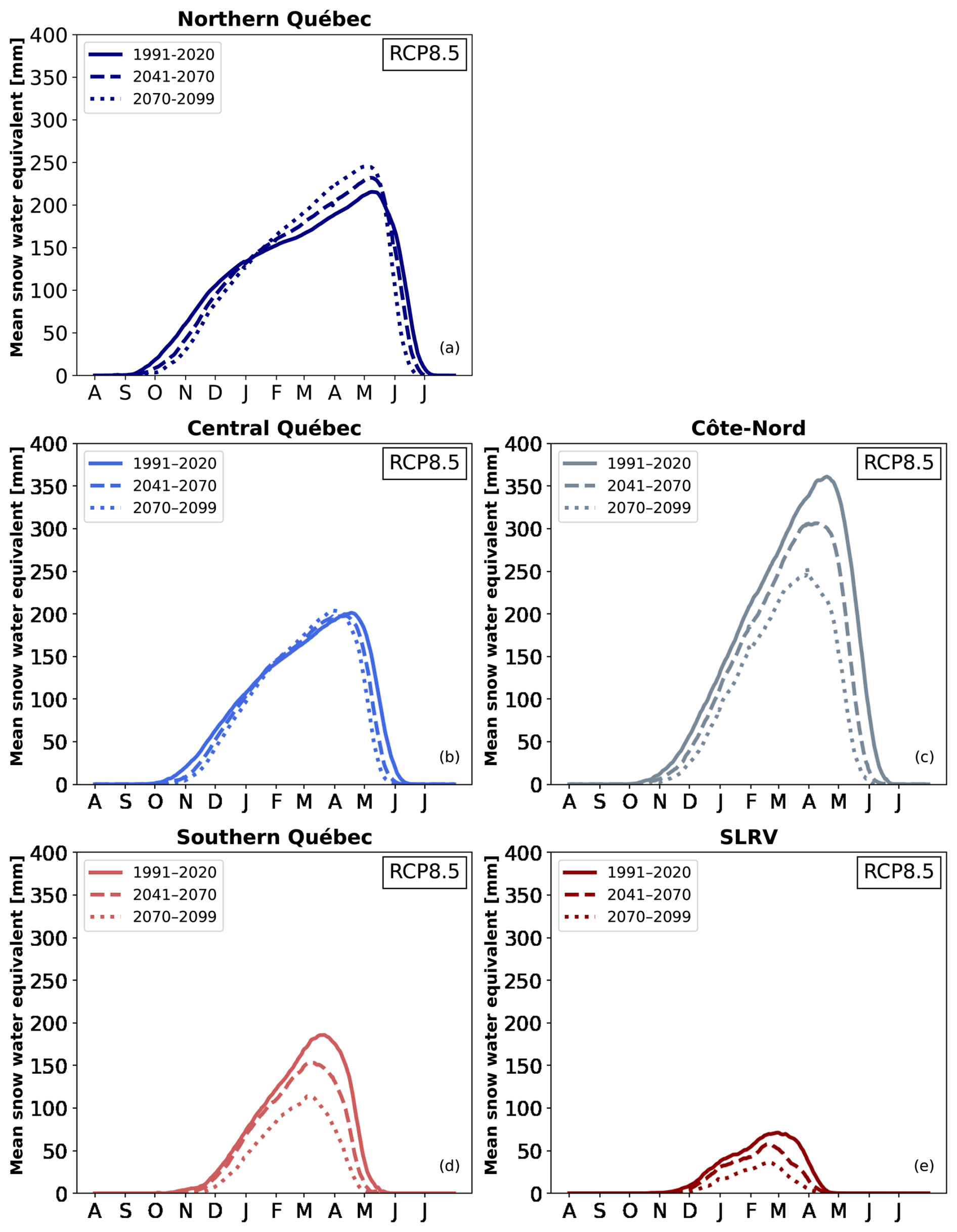
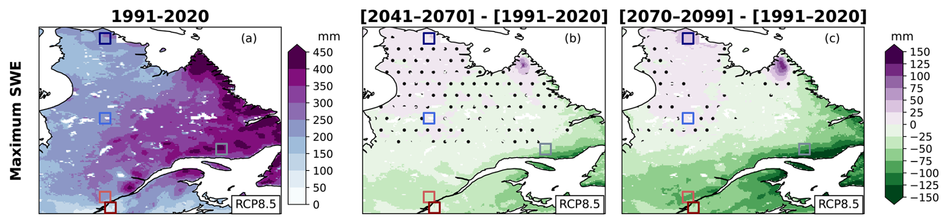
Figure 9 Annual maximum SWE for 1991–2020 (a), and differences between the 1991–2020 period and 2041–2070 (b) or 2070–2099 (c). Dotted areas are those where less than 80 % of the simulations in the ensemble agree on the sign of change. Results are presented for the RCP8.5 ensemble.

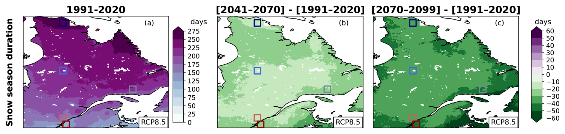
Figure 10 Annual snow season duration for 1991–2020 (a), and differences between the 1991–2020 period and 2041–2070 (b) or 2070–2099 (c). Dotted areas are those where less than 80 % of the simulations in the ensemble agree on the sign of change. Results are presented for the RCP8.5 ensemble.

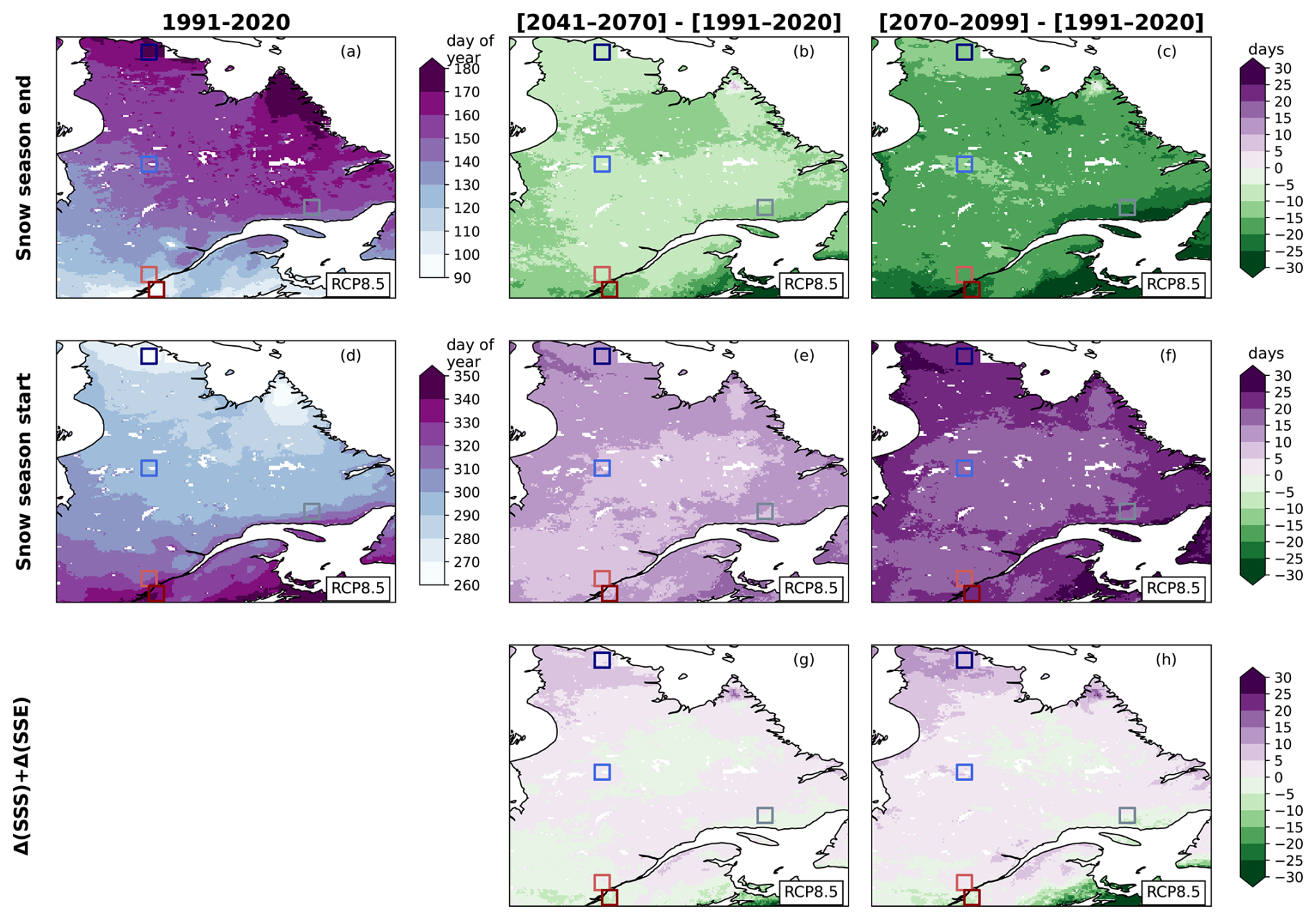
Figure 11 Snow season end (a, b, c), snow season start (d, e, f) and the sum of the change in timing of snow season start and change in timing of snow season end (g, h), for 1991–2020 (a, d), and differences between the historical period (1991–2020) and 2041–2070 (b, e, g) and 2070–2099 (c, f, h). Results are presented for the RCP8.5 ensemble.

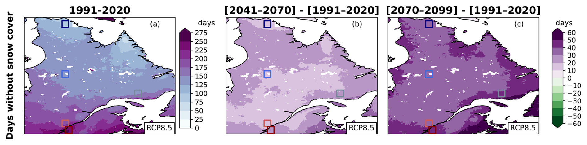
Figure 12 Annual days without snow cover for 1991–2020 (a), and differences between the 1991–2020 period and 2041–2070 (b) or 2070–2099 (c). Dotted areas are those where less than 80 % of the simulations in the ensemble agree on the sign of change. Results are presented for the RCP8.5 ensemble.

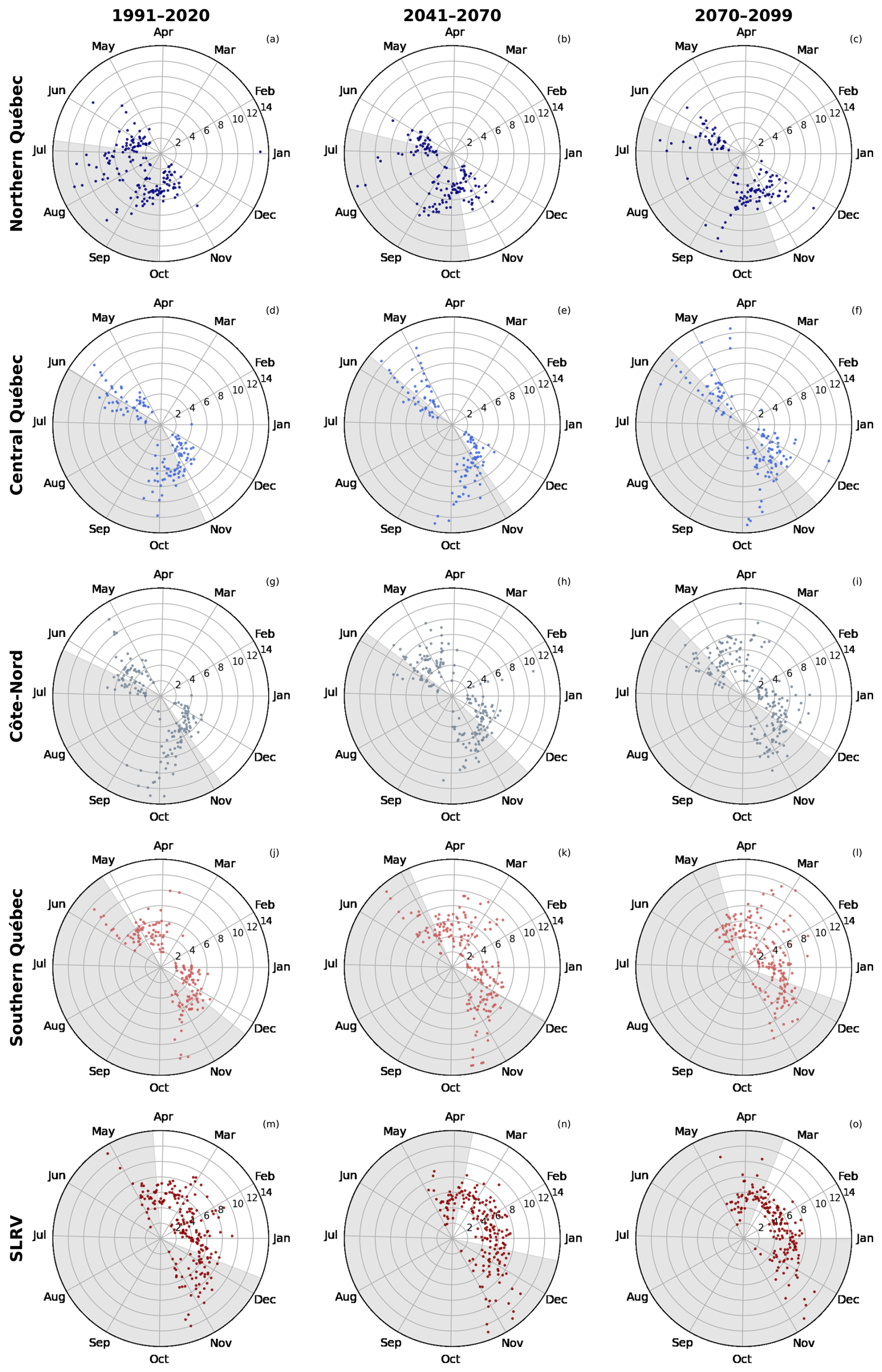
Figure 13 Length of sequences of 2 to 13 consecutive days without snow cover (radius) as a function of the day of the year (angle) for the RCP8.5 ensemble. The white part of each figure is the mean snow season for the studied period and region. The months are labelled on the first day of the month. Results are presented per region (rows) and for 1991–2020 (left), 2041–2070 (centre) and 2070–2099 (right).

Figure 5 shows the distribution of biases for each station, which are sorted with their elevation. Only stations with observations during January and April are considered. At elevation higher than 150 m, even if the median bias is near 0, when the bias is positive, its amplitude can reach large values (larger than for negative biases) (Fig. 5a). The seasonality of the snow cover is important, and the bias is not constant in time (Fig. 5b, c). Indeed, SWE is better estimated by ERA5-Land during January (Fig. 5b) and February (not shown), than in March (not shown) and April (Fig. 5c). April results show more variability in the bias of magnitude, leading to the hypothesis that ERA5-Land has more difficulty reproducing the end of the season accurately, especially with melting processes slower than observed.

3.2 Snow cover climatology

The snow cover climatology of the historical period (1991–2020) is analyzed for ERA5-Land (Fig. 6a, d, g). SWEmax is larger over the eastern part of Québec and Labrador (e.g. 375 mm for Côte-Nord), and particularly over mountainous regions like the Gaspesian peninsula, Charlevoix, or the Torngat Mountains (presented in Fig. 1) than the rest of the domain (e.g. 216 mm for central Québec) (Fig. 6a). The plains in the south of the domain (SLRV) show the smallest maximum SWE (107 mm), about 100 mm less than the mountainous region at a similar latitude (southern Québec region). Meanwhile, a South-North gradient is noticeable for SSD, SSS, SSE and noSC (Figs. 6d, g, 7a). For example, the northern Québec region experiences long SSD (273 d), few noSC (90 d) (Fig. 6d, g), and has a snow season that begins late September and ends late June (Fig. 7a). In comparison, the southern Québec region has a short snow season (SSD; 166 d), starting in mid-November and ending in early May, and 196 d without snow cover (noSC) (Figs. 6d, g, 7a). This meridian gradient is also observed when looking at the date when the maximum of SWE happens: from mid-May in northern Québec to late March in southern Québec (Fig. 8a, b, d).

In general, the RCP4.5 and RCP8.5 ensembles present the same portrait for all indices on the historical period (Figs. 6b, e, h, 7b, S3b, e, h, S4). Relative biases of the ensembles compared with ERA5-Land are globally ±5 % for SWEmax, SSD and noSC indices (Figs. 6c, f, i, S3c, f, i). In the southern part of the domain, the positive bias reaches 10 % to 15 % for SWEmax (Fig. 6c).

3.3 Projected changes in snow cover

The future periods studied hereafter are 2041–2070 (1 August 2041–31 July 2071) and 2070–2099 (1 August 2070–31 July 2100). Consensus between the simulations presented in Figs. 9–12 (as well in Figs. S6–S9) is reached when 80 % of the simulations agree on the sign of change. In other words, the consensus is reached for RCP4.5 ensemble when 4 simulations out of 4 (100 %), and for RCP8.5 ensemble when 5 out of 6 (83 %) simulations agree on the sign of change. This unbalance needs to be taken in consideration, as this consensus criterion is stricter, in practice, for RCP4.5 than for RCP8.5 ensemble. Nevertheless, there are no noticeable changes in the consensus when the threshold is set to 75 % instead of 80 %, except for SWEmax that presents more consensus in the region where the sign of the difference in future and past climatology changes with RCP4.5 ensemble (not shown). The two RCP ensembles present similar trends, but the magnitude of change is smaller for the RCP4.5 ensemble than for RCP8.5. Only the results of the RCP8.5 are presented here to streamline the text. The results for the RCP4.5 ensemble are available in Figs. S3–S9.

As time progresses, the magnitude of SWEmax increases in Nunavik and the Torngat Mountains, is stable for central Québec, and decreases for the other regions (Figs. 8, 9). More than 80 % of the simulations in the ensemble agree on the sign of change in Nunavik, the Torngat Mountains, and the southern half of the domain. This change is consistent with the projected increase in precipitation and temperature in Québec (Bush and Lemmen, 2019). The timing of SWEmax also changes: the annual cycle of SWE shows that the maximum SWE occurs earlier (a change of about 6 to 10 d between 1991–2020 and 2070–2099) for four regions (Fig. 8a–d), while the signal is more ambiguous for the SLRV region (Fig. 8e).

The annual SWE cycle also shows a decrease in the duration of the snow season (Fig. 8). The change in SSD is almost spatially homogeneous, with a decrease of about 0 to −20 d [−20 to −50] for 2041–2070 [2070–2099] relative to 1991–2020 (Fig. 10). More than 80 % of the simulations in the ensemble agree with the decrease. The SSD shrinkage is quite symmetrical as presented in the changes in SSS and SSE, except for the northern part of Québec (Figs. 7, 11). In this region, the change in the SSS is larger than the change in the SSE but never exceeds 15 d (Fig. 11g, h). This change is more significant for 2070–2099 than for 2041–2070. This can be related to the iso-0 °C line moving northward. A large part of the domain experiments a warming that affects the snow season limits (SSS and SSE), but this warming is weaker in the northern part of Québec for these moments of the year, especially at the end of the season during the months of May and June (e.g. Leduc and Logan, 2025). Historically, there are years where there is a barely a pause in snow cover, and a partial thin snow cover below the 4 mm threshold used for SSS and SSE indices can still give an albedo that helps a snow build-up in the start of seasons. With climate change, it becomes more likely that Northern Quebec experiments a more frequent total absence of snow, which further delays snow season starts. The phenomenon may also explain why the SSE for the Côte-Nord region becomes closer to the one of central Québec as time passes (Fig. 7).

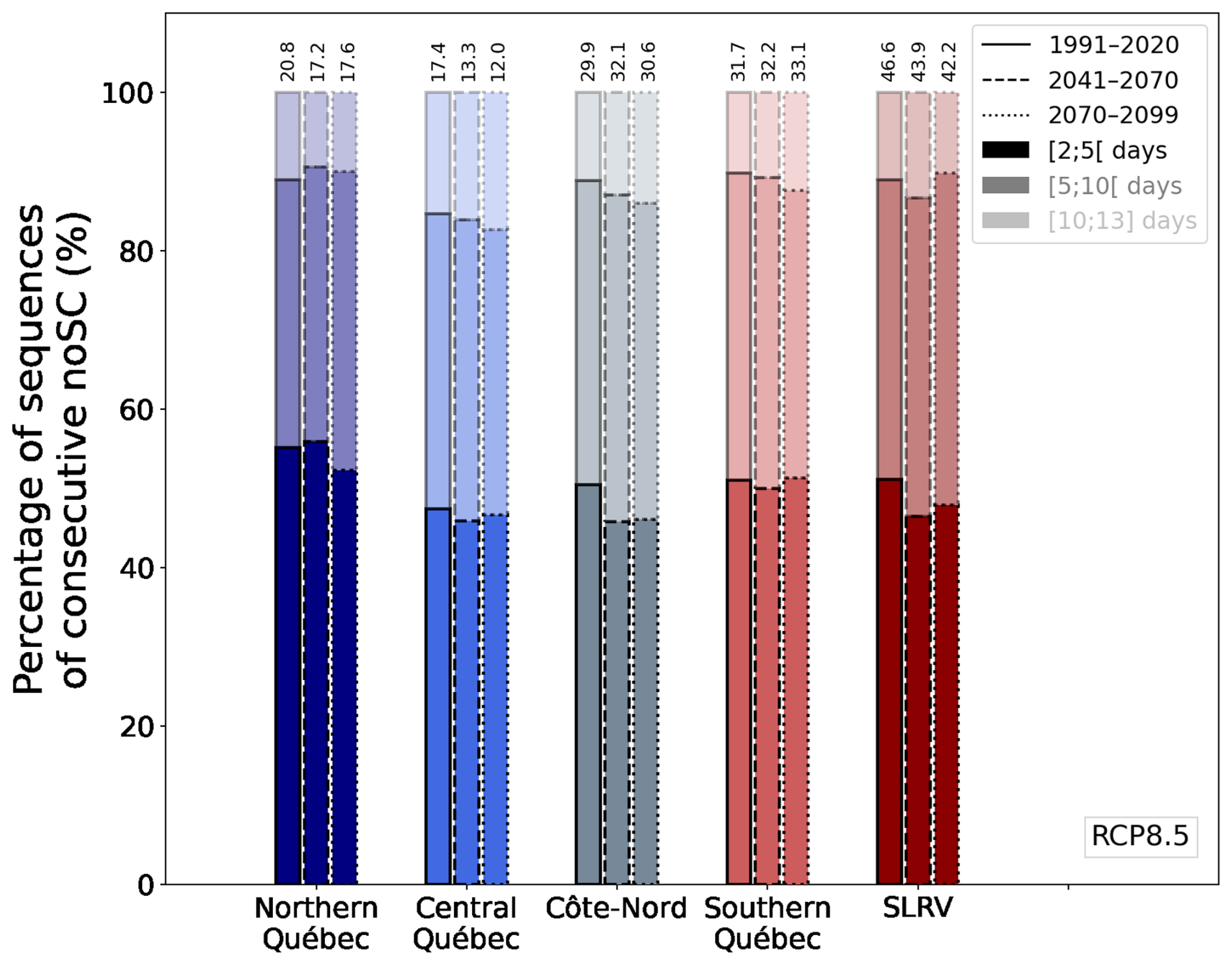
Figure 14 Percentage of noSCseq during the snow season for the historical period 1991–2020 (lines), 2041–2070 (dashed lines) and 2070–2099 (dotted lines) for the five regions of interest. Three duration ranges are presented with different transparencies: [2; 5[, [5; 10[ and [10; 13] consecutive days for the RCP8.5 ensemble. Values on the top of each bar correspond to the total number of noSCseq during the snow season for each region and period.

Over time, noSC increases by approximately 0 to +20 [+20 to +50] d for 2041–2070 [2070–2099] (Fig. 12). The coastal regions gain more snow-free days than continental regions, which could be a result of a larger warming in the coastal regions where there are comparatively less mountains. The spatial pattern of noSC is preserved for all periods. This increase in noSC could be the result of (1) the shrinkage of the snow season (Fig. 10); (2) changes in the distribution of days without snow cover during the snow season. To investigate the second point, we use the noSCseq indicator presented previously. Figure 13 shows the day of the year (angle) and the average length of noSCseq starting on that day (radius), superposed on the mean snow season (white area) for each 30-year period. During the historical period, fragmentation rarely occurs during January or February, except in the SLRV region. No changes in January and February are projected for the northern and central Québec regions (Fig. 13a–f). For the other regions, the number of days with a noSCseq increases in January and February. The projected increase in temperature may explain the presence of noSCseq in January and February for the Côte-Nord, southern Québec, and SLRV regions. As already shown, the season shortens, so this result is expected.

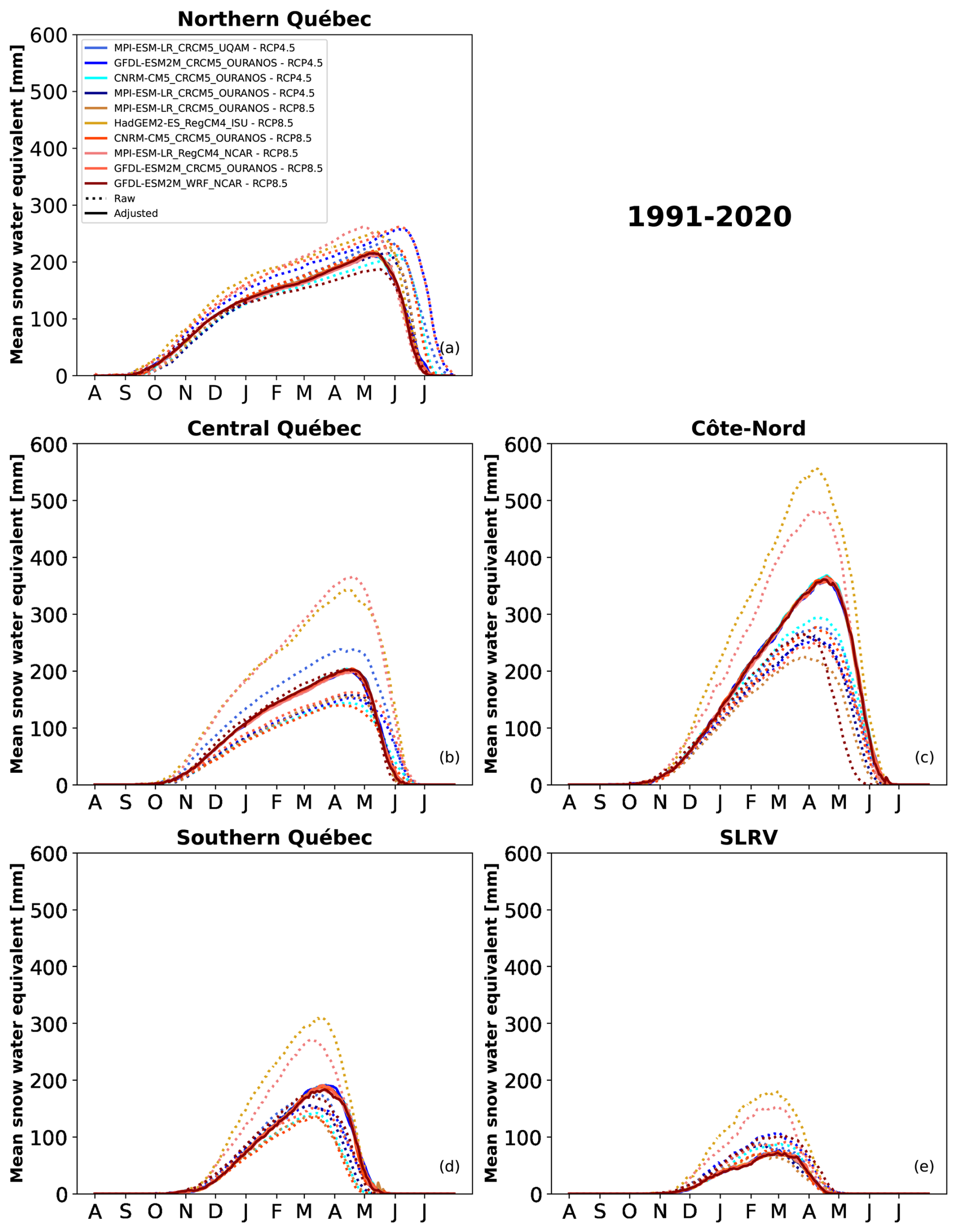
Figure 15 Mean annual cycle of SWE for the five regions of interest for 1991–2020. Raw simulations are represented with dotted lines, and adjusted ones with solid lines. Each colour corresponds to a simulation.

4 Discussion

4.1 Bias adjustment effect on annual cycle

After the first selection of simulations discussed in Sect. 2.3.2, inter-model differences remain, especially in the SWE amplitude. Figure 15 presents the differences between the climatology (1991–2020) of the annual cycle of SWE for raw (dotted line) and bias adjusted (solid line) simulations for the five regions of interest. The raw simulations were downscaled to ERA5-Land grid using a bilinear interpolation.

The subregion with the larger discrepancies in raw simulations is Côte-Nord with maximum SWE from around 200 to 550 mm. The simulations produced with the RegCM4 model present a larger amount of SWE than the other simulations, except for Northern Québec. This is coherent with McCrary and Mearns (2019) conclusions on the bias in RCM’s SWE being mostly induced by the RCM, less by the GCMs.

As expected, bias adjustment mainly influences the SWE amplitude, and in a smaller part the SSS and SSE. The bias adjustment succeeds in reducing the small systematic bias from GCMs or inherited by RCMs from their drivers and helps reduce inter-model differences.

4.2 Comparison between RCP ensembles and simulations

All figures shown above are available for the RCP4.5 ensemble in the Supplement (Figs. S3–S11). In general, trends are similar for both ensembles, with more significant changes for the RCP8.5 ensemble than for RCP4.5. The RCP4.5 ensemble has fewer sequences of consecutive days without SWE than the RCP8.5. All of this can be related to a smaller warming in the RCP4.5 ensemble, as expected.

When simulations are individually analyzed (instead of the median of the ensemble called RCP ensemble), different spatial patterns can be noted but as presented in Figs. 11 and 12, there is good agreement between them regarding the trends (see Figs. S12–S19) regardless of the RCP ensemble. However, this does not apply to SWEmax, where a larger spread between members is seen for both ensembles with large regions where less than 80 % of the members agree on the sign of change.

4.3 Indices defined with a threshold

In the list of indices analyzed in this study, only SWEmax does not depend on a threshold. The other ones are conditional to the presence/absence of a snow cover, which is defined here as when SWE ≥4 mm. First, the choice of the threshold itself for the snow cover definition is somewhat arbitrary. Depending on the literature on which we rely, the snow cover threshold can have different values: 1 mm (Brown et al., 2010), 2.54 mm (0.1 in.) (McCrary and Mearns, 2019), 4 mm (Mudryk et al., 2017), or 5 mm (Brutel-Vuilmet et al., 2013). A sensitivity study to different thresholds would be of interest in future work but is not within the scope of the present article. Secondly, even if it was shown above that ERA5-Land performs better than other products for our studied domain and for SWE, it still has biases (see Sect. 2.3.1). Given the impact this can have, notably on indicators with thresholds, new or updated reference products with less biases should be taken in consideration in the future.

5 Conclusions

Snow cover is an important parameter for the evolution of climate in Canada. It has effects on ecology, agriculture, and many sectors of activity. Stakeholders and decision makers need useful data that is easily accessible and stored in a convenient format. In this study, we produced a portrait of useful snow cover indices for the Québec region. To achieve this result, we selected regional climate model simulations, applied a statistical bias adjustment to the simulated SWE, computed snow cover indices, and analyzed them. The overview of the snow cover change in northeastern Canada shows a shortening in the snow season, with similar, symmetrical changes for both the start and the end of the season, as well as a decrease of the maximum of SWE everywhere, except in the northernmost part of Québec (Nunavik and Torngat Mountains). Côte-Nord, southern Québec and SLRV regions experiment a more fragmented snow season (consecutive days without snow cover during the season) than the northern and central Québec regions. These results are consistent with those of the literature (e.g. Brown and Mote, 2009; Shi and Wang, 2015; Mudryk et al., 2020; McCrary et al., 2022).

This study suffers from a few limitations: the selection criterion is sensitive to the domain, the resulting ensemble of simulations is quite small and the SWE threshold used to define snow cover is somewhat arbitrary. The use of an external snow model could have been an alternative to produce this data by considering all regional climate model simulations that have archived the required variables. The choice was made to use SWE simulated with the land surface model coupled to regional climate models in an attempt to preserve the physical interactions and feedback between atmospheric and surface variables. The application of a bias adjustment has impacted these interactions which could affect physical coherence when this dataset is used with other adjusted climate variables. A follow-up study could be useful to investigate the difference between our results and those produced with different land surface models in offline-mode using atmospheric input from the same regional climate simulations. This study could be extended to other regions. Precautions will have to be taken for mountainous regions like the Rocky Mountains, as the focus of the article was northeastern Canada which has a lower topography than western Canada. SWE behaviour in mountainous regions in regional climate models as well as in reanalyses can present some challenges.