Mesoscale ice–atmosphere–ocean coupling processes drive interannual-to-decadal timescale shift of Bering Sea January sea ice variability

Over the past four decades, the sea ice area (SIA) in the Bering Sea has shifted from interannual to decadal variability, manifested as persistent heavy-ice or light-ice regimes. However, the mechanisms driving this shift remain unclear. This study demonstrates that the initial shift occurs in January and is triggered by the December SIA anomalies. Specifically, December SIA anomalies induce substantial modifications in localized air-sea heat flux, triggering mesoscale vertical air movements. This process generates localized anticyclonic wind field anomalies during heavy-ice years and anomalous cyclonic wind field anomalies during light-ice years. Subsequently, these mesoscale dynamic processes activate negative feedback in the atmosphere and positive feedbacks in the ocean, which differentially regulate wind divergence and northward heat transport. The former produces out-of-phase variations between December SIA and January SIA increment (ΔSIA), contributing to interannual variability in January SIA, whereas the latter exhibits significant decadal variability over the past two decades, inducing in-phase changes that amplify decadal-scale signals in sea ice variability. The study emphasizes the critical role of mesoscale ice–atmosphere–ocean coupling processes and their profound impacts on regional oceanic dynamics and sea ice evolution. Given the observed decadal-scale regime shifts in sea ice, of paramount importance and urgency is to assess the implications of sustained heavy/light ice conditions on local ecosystems, indigenous communities, and commercial fisheries.

1 Introduction

Bering Sea has experienced a long-term low record of winter sea ice area (SIA) since 2014 (Hunt et al., 2022; Iida et al., 2020; Thoman et al., 2020; Wang et al., 2022, 2023, 2024). In the winter of 2018, the maximum SIA plummeted to 1.68×10⁵ km², constituting a mere 30.8 % of the historical average (Wang et al., 2023) . This sustained ice loss has triggered profound changes in regional hydrology, meteorology, ecosystems and even socioeconomic dynamics (Thoman et al., 2020; Wyllie-Echeverria and Wooster, 1998), including weakened seawater stratification (Kinney et al., 2022; O'Leary et al., 2022), delayed spring blooms (Huntington et al., 2020; O'Leary et al., 2022), diminished abundance of large crustacean zooplankton (Belkin and Short, 2023; Hermann et al., 2021; O'Leary et al., 2022; Stabeno and Bell, 2019), and shrinkage or complete disappearance of the cold pool (Kinney et al., 2022; Stabeno and Bell, 2019). Furthermore, reduced SIA in the Bering Sea has been linked to amplified extreme climate events across mid-and high-latitudes of the Northern Hemisphere, with pronounced impacts on Northeast Asia and North America (Iida et al., 2020; Li and Wang, 2013; Ma and Zhu, 2022; Vihma, 2014; Wu et al., 2009; Zhao et al., 2004; Zhou and Wang, 2008, 2014). Scientists anticipate that the Bering Sea could be ice-free in winter as early as in the next decade (Iida et al., 2020).

Prior to the recent light-ice years, the Bering Sea experienced a decade-long surge in winter SIA. In 2012, the SIA exceeded the historical average by 55.4 % and the highest level since satellite monitoring began in 1979 (Stabeno et al., 2012a, b; Wu and Chen, 2016). The climate regime demonstrates distinct decadal oscillations, alternating between several years of relatively extensive sea ice formation and cold summer temperatures (e.g., 2006–2013) and several years of minimal sea ice formation and warm summer temperatures (e.g., 2002–2005, 2014–2021) (Overland et al., 2012; Stabeno et al., 2012a, b; Stevenson and Lauth, 2019; Wang et al., 2022; Yang et al., 2020). This shift contrasts with earlier predominantly interannual/multiyear SIA variability. Prior research has indicated that hydrological changes in the Bering Sea shelf occur on at least two-time scales – interannual and multi-year (Wyllie-Echeverria and Wooster, 1998). Overland et al. (2012) examined the 95-year air temperature record from St. Paul Island in the Bering Sea shelf and determined that decadal warm or cold events are rare and of a random nature. Wu and Chen (2016) pointed out that at the beginning of this century, the Bering Sea SIA in March exhibited significant decadal variation characteristics. According to Yang et al. (2020), the decadal variability in March SIA over the Bering Sea began in 2007 and was caused by the phase-locking of the North Pacific Gyre Oscillation (NPGO) and the Pacific Decadal Oscillation (PDO). According to Wang et al. (2022), the decadal variability of January SIA increment (the SIA in January minus the SIA in December of the previous year) in the Bering Sea may have started in 1994 and is closely related to the northward heat transport over the Bering Sea shelf.

The winter spatial patterns of sea ice coverage in the Bering Sea have been metaphorically described as a “conveyor belt”, wherein ice is transported from northern source to southern sink through an intermediate zone (Li et al., 2014; Niebauer et al., 1999; Pease, 1980; Wang et al., 2024). Persistent northerly winds drive the ice southward, while ocean heat transport restricts its further southward advance (Brown and Arrigo, 2012; Li et al., 2014; Stabeno et al., 2007; Wang et al., 2022; Zhang et al., 2010). Although previous studies have identified key drivers of Bering Sea ice variability – including atmospheric circulation anomalies (Niebauer, 1980, 1988, 1998; Niebauer et al., 1999; Sasaki and Minobe, 2005), frequent storms (Mesquita et al., 2010; Rodionov et al., 2007; Screen et al., 2011), ice intake from the Arctic Ocean (Babb et al., 2013; Zhang et al., 2010), and poleward oceanic heat transport (Wang et al., 2022, 2023) – there remains a notable absence of comprehensive discussions on these impact factors. This gap impedes a holistic understanding of sea ice variability in the Bering Sea, making it much more challenging to comprehend the underlying causes of the timescale transition of sea ice change.

In essence, Bering Sea SIA variability is intricately shaped by a blend of thermodynamic and dynamic processes. Thermodynamically, ice growth and melt are governed by atmosphere-ice and ocean-ice heat exchange. Dynamically, ice convergence/divergence drives local SIA variability. Seasonally, northern Bering Sea ice changes are dominated by atmospheric surface heat flux, while southern ice edge variability is controlled by ice-ocean heat flux (Li et al., 2014). Wind-driven ice transport further modulates spatial patterns (Li et al., 2014; Zhang et al., 2010). In the context of recent Arctic amplification, reduced meridional sea level pressure (SLP) gradients have weakened westerly winds (Cao and Liang, 2018; Dai et al., 2019; Gramling, 2015; Shepherd, 2016), while enhanced northward heat transport through the Bering Strait (Danielson et al., 2014; Woodgate and Aagaard, 2005; Woodgate and Peralta-Ferriz, 2021) complicates the wind-ice coverage relationship. These substantial changes occur simultaneously with transitions in SIA variability timescales. A comprehensive analysis and thorough examination are requisite to discern the extent to which they function as driving forces in the timescale transition of sea ice. This article endeavours to tackle two core issues: (1) Unravelling the causes of SIA variability at interannual versus decadal timescales; (2) Investigating the variables responsible for the timescale transition in SIA. The primary emphasis of this study centres on the examination of the SIA in the Bering Sea during the month of January, a topic that will be comprehensively expounded upon subsequently. The manuscript is organized into five sections: The initial section provides clarity on the background and motivations, while the second section meticulously delineates the materials and methods employed in the research. The third section delineates the rationale for investigating SIA in January and expounds upon its primary spatiotemporal characteristics. Additionally, it offers an initial elucidation of the factors contributing to the transition of SIA increment from an interannual to a decadal timescale in January. The fourth section systematically unveils the underlying physical mechanisms governing the timescale transition of sea ice in January. The conclusive section summarizes the key findings and contributions of this article.

2 Materials and methods

2.1 Materials

We utilize monthly mean NASA-team satellite sea ice concentration (SIC) data derived from the Scanning Multichannel Microwave Radiometer (SMMR), Special Sensor Microwave/Imager (SSM/I), and Special Sensor Microwave Imager/Sounder (SSMIS) (Comiso, 2000). The SIC data is obtained at a spatial resolution of 25 km. To calculate SIA, grid-cell area-weighted SIC values were spatially integrated across the area of interest (51–66° N, 165–205° E). We then derived year-to-year January SIA increment (ΔSIA) and constructed a continuous time series spanning 1979–2023. We also utilized Hadley Centre Sea Ice and Sea Surface Temperature dataset (HADISST) (Rayner et al., 2003) as supplementary validation to confirm the robustness of timescale shift in the January ΔSIA from interannual to decadal variability.

We applied Empirical Orthogonal Function (EOF) analysis to extract the dominant spatial patterns (EOFs) and their corresponding time series (PCs). To quantify the relative importance of the first two EOF modes in driving January ΔSIA variability, we compared their principal component ($\frac{{\text{PC}}^{\mathrm{2}}\left(k\right)}{{\mathit{\lambda }}_k}$, $k=\mathrm{1},\mathrm{2}$, where λ_k denotes the eigenvalue). The Maximum Overlap Discrete Wavelet Transform (MODWT) was implemented to decompose the time series of January ΔSIA into multiscale components, enabling explicit identification of timescale transitions in sea ice variability. We systematically analysed the linkages between atmospheric processes in December and concurrent SIA through composite analysis and regression analysis. Causal relationships were quantified using the information-flow theory proposed by Liang (2014), while the impacts of December wind field anomalies and oceanic heat flux on subsequent ΔSIA were assessed through lagged correlation analysis.

We employed the satellite products and reanalysis data to reconstruct the surface currents within the Bering Sea. The key datasets include: (1) the NOAA optimum interpolation SST (OISST) product at 0.25° resolution, as expounded upon by Reynolds et al. (2007); and (2) the Topex/Poseidon and European Remote-sensing Satellite (ERS) altimetric dynamic topography products, also on a 0.25° × 0.25° grid, as made available by AVISO (2013). Additionally, atmospheric variables – surface air temperature (SAT), omega, sea level pressure (SLP), wind vector at 10 m, latent heat net flux, net longwave radiation flux, net shortwave radiation flux and sensible heat net flux – were obtained from the National Centers for Environmental Prediction/Department of Energy Atmospheric Model Intercomparison Project (NCEP/DOE AMIP-II) reanalysis (Kanamitsu et al., 2002). The net air-sea heat flux is computed as the summation of four individual components with upward fluxes defined as positive (ocean heat loss). To validate robustness, we conducted additional verification using ERA5 reanalysis data provided by ECMWF (Figs. S1–S4 in the Supplement). Our validation process demonstrated that the results obtained from both datasets are consistent. In this study, we primarily focus on the results derived from NCEP/DOE reanalysis data, while the complementary findings from ERA5 are available in the Supplement.

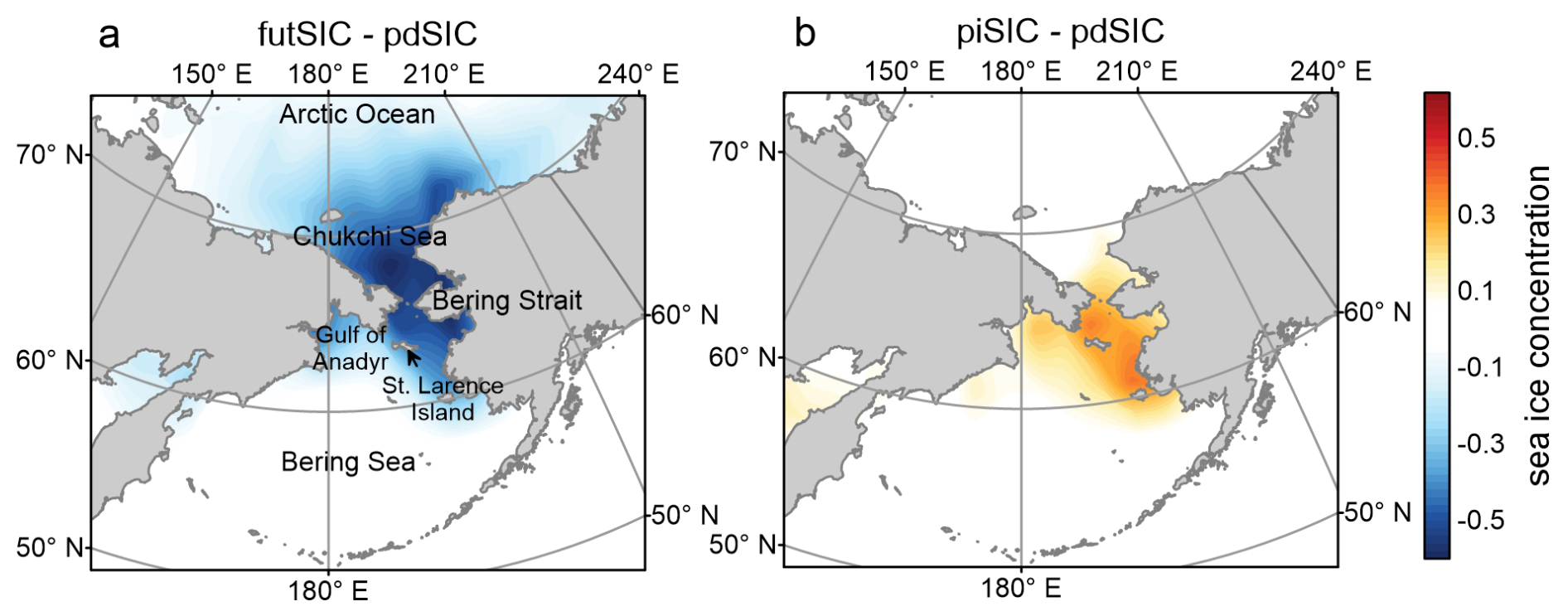
Figure 1 Spatial comparison of Bering Sea sea ice concentration (SIC) anomalies from Community Earth System Model version 2 (CESM2) simulations under two contrasting climate forcing scenarios: (a) future (futSIC) and (b) pre-industrial (piSIC). All SIC anomalies are computed relative to the present-day (pdSIC) climatological mean SIC over the study domain.

In order to investigate SLP responses to extreme sea ice conditions in December (Fig. 1), we analysed the Polar Amplification Intercomparison Project (PAMIP) experiments under CMIP6 using the CESM2 model (Danabasoglu, 2019). Specifically. three tier-1 time slice experiments were evaluated: (1) pdSST-pdSIC, prescribed 1979–2008 climatological SIC; (2) pdSST-piArcSIC, pre-industrial Arctic SIC representing extreme heavy-ice years (Fig. 1b), and (3) pdSST-futSIC, RCP8.5-projected Arctic SIC representing extreme light-ice years (Fig. 1a). All experiments used fixed climatological SST with 1 April 2000 initial conditions, running 14 months (2-month spin-up discarded). December–January outputs from the final 12 months were analysed to quantify SLP anomalies induced by contrasting sea ice states.

In an effort to further expand our analysis, we have incorporated surface and bottom water temperature data obtained from in situ observational records. These data were collected during bottom trawl surveys conducted by the NOAA/AFSC/RACE's Groundfish Assessment Program in the eastern Bering Sea. We accessed this valuable dataset through the technical report published by Rohan et al. (2022). By including these water temperature measurements, we aim to provide a more comprehensive understanding of the timescale transition in the entire marine environment of the Bering Sea.

2.2 Methods

2.2.1 Sea ice area increment (ΔSIA) and maximum SIA

In this study, we focus on the January ΔSIA to assess the influence of atmospheric or oceanic forcing from the preceding month on sea ice variability. The SIC change is calculated as the difference between the current and preceding monthly SIC values for each grid cell. The January ΔSIA is then derived by applying area-weighting to grid cell-level SIC changes, followed by spatial integration across the region of interest (51–66° N, 165–205° E). Anomalies are obtained by subtracting the climatological mean of the corresponding month. Through comparison of monthly SIA values, the annual maximum SIA in the Bering Sea is identified as the peak value within the annual observational record.

2.2.2 Maximal Overlap Discrete Wavelet Transform (MODWT) method

The Maximum Overlap Discrete Wavelet Transform (MODWT) is utilized to perform the multiresolution analysis of January ΔSIA. As an extension of the Discrete Wavelet Transform (DWT) commonly used in signal processing, MODWT operates as a time-invariant transform (Walden and Contreras Cristan, 1998). Distinct from DWT, MODWT, devoid of a downsampling process, minimizes the risk of input signal loss. An advantageous feature of MODWT is its lack of stringent data length requirements, enhancing low-frequency information in multiresolution decomposition. Consequently, the MODWT methodology is applied to decompose the January ΔSIA time series into interannual (1–3 years), multi-year (4–8 years), and decadal scales (8–16 years). To quantify the dominance of variability at each scale, the study calculates relative energy contributions at distinct timescales.

2.2.3 Composite analysis

Following the EOF analysis of the January ΔSIA, the observational period is categorized into three ice-condition classes based on the normalized December SIA (nSIA₁₂): normal year (NM, $-\mathrm{1}\le {\text{nSIA}}_{\mathrm{12}}\le \mathrm{1}$), heavy-ice year (HI, nSIA₁₂>1), and light-ice year (LI, nSIA${}_{\mathrm{12}}<-\mathrm{1}$). Composite differences, encompassing variables such as SIC, net air-sea heat flux, SST, SAT, and wind vectors, were then derived for each category. Further details can be found in Sect. 3.2.

2.2.4 Oceanic northward heat transport

In this study, surface wind vectors and oceanic northward heat transport (NHT) are employed to characterize atmospheric and oceanic forcing factors, respectively. We systematically explore their association with the January ΔSIA across various timescales. The formula for computing NHT is delineated as follows:

$$\begin{array}{}\text{(1)}& \text{NHT}=\underset{{\mathit{\lambda }}_{\mathrm{1}}}{\overset{{\mathit{\lambda }}_{\mathrm{2}}}{\int }}\underset{-H_{\mathrm{MLD}}}{\overset{\mathrm{0}}{\int }}\mathit{\rho }{c}_{p}vTr\text{cos}\mathit{\theta }\mathrm{d}z\mathrm{d}\mathit{\lambda }\end{array}$$

where ρ=1022.95 kg m⁻³ is the density of seawater; c_p=3900 J kg⁻¹ K⁻¹ is the specific heat capacity of seawater; v is the meridional surface current; r=6371 km is the radius of the Earth; θ is the latitude, and λ is the longitude. In this study, ρ, c_p, and r are constant, which means that NHT is proportional to vTH_MLDcosθ. T is the SST derived from the mean temperature within the depth H_MLD (the mixed layer depth).

Prior to calculating NHT, the sea surface velocity vector (V(u, v)) must be determined. It is approximated as the sum of surface geostrophic current (V_ge) and the wind-driven Ekman velocity (V_ek). We employed sea surface dynamic height and wind vectors data to compute surface currents, with the calculation equation articulated as follows:

$$\begin{array}{}\text{(2)}& {\displaystyle }{\mathit{V}}_{\mathbf{ek}}={\displaystyle \frac{\mathrm{1}}{{\mathit{\rho }}_{\mathrm{0}}f}}\left({\mathit{\tau }}_y,-{\mathit{\tau }}_x\right)\text{ and }\mathit{\tau }={\mathit{\rho }}_{\mathrm{0}}{C}_{\mathrm{D}}\left|{\mathit{u}}_{\mathrm{s}}\right|{\mathit{u}}_{\mathbf{s}}\text{(3)}& {\displaystyle }{\mathit{V}}_{\mathrm{ge}}={\displaystyle \frac{g}{f}}\left(-{\displaystyle \frac{\partial h}{\partial y}},{\displaystyle \frac{\partial h}{\partial x}}\right)\end{array}$$

where ρ₀=1.25 kg m⁻³ is the air density, C_D=0.00125 is the drag coefficient, f is the Coriolis parameter, g=9.8 m s⁻² is the acceleration of gravity, and h is the dynamic topography. The subscripts “x” and “y” of τ denote the zonal and meridional directions, respectively. u_s is obtained, as described above, from the wind data recorded at 10 m above sea level. This methodology has been extensively validated in oceanic dynamical studies (Dohan and Maximenko, 2010; Sudre and Morrow, 2008; Wang et al., 2024). Wang et al. (2024) offers a comprehensive evaluation of the uncertainty associated with ocean heat transport using this approach.

To unravel the causal links between SIA and atmospheric processes, we implement two complementary approaches: moving-window correlation coefficient (MCC) and Liang-Kleeman information flow analysis. A two-sided Student's t-test was employed to evaluate the statistical significance of the MCC, ensuring a rigorous assessment of the results. The degrees of freedoms is N_eff−2. $N_{\mathrm{eff}}=N/(\mathrm{1}+\mathrm{2}\sum _{i=\mathrm{1}}^{N-\mathrm{1}}\frac{N-i}{N}{\mathit{\rho }}_{x,i}{\mathit{\rho }}_{y,i})$ is the number of effective degrees of freedoms of the combined dataset, where N denotes the sample size and ρ_x,i is the auto-correlation of time series x with lagi (Bayley and Hammersley, 1946). Here, our primary focus lies in the Liang-Kleeman information flow,

2.2.5 Liang-Kleeman information flow

Liang and Kleeman have pioneered the introduction of the information flow method as a means to unveil causal relationships embedded within time series data (Liang, 2014). For two given series, X₁ and X₂, the rate of information flow (expressed in units of nats per unit time) from the latter to the former is defined as follows:

$$\begin{array}{}\text{(4)}& T_{\mathrm{2}\to \mathrm{1}}={\displaystyle \frac{C_{\mathrm{11}}{C}_{\mathrm{12}}{C}_{\mathrm{2},d\mathrm{1}}-C_{\mathrm{12}}^{\mathrm{2}}{C}_{\mathrm{1},d\mathrm{1}}}{C_{\mathrm{11}}^{\mathrm{2}}{C}_{\mathrm{22}}-C_{\mathrm{11}}{C}_{\mathrm{12}}^{\mathrm{2}}}}\end{array}$$

where C_ij is the sample covariance between X_i and X_j, C_i,dj is the covariance between X_i and $\dot{X_j}$, and $\dot{X_j}$ is the difference approximation of $\frac{\mathrm{d}{X}_j}{\mathrm{d}t}$ using the Euler forward scheme:

$$\begin{array}{}\text{(5)}& {\dot{X}}_{j,n}={\displaystyle \frac{X_{j,n+k}-X_{j,n}}{k\mathrm{\Delta }t}}\end{array}$$

where k≥1 but should not be too large to ensure precision. Practically, a comparison can first be made between the results with k=1 and k=2. If the results are qualitatively different, then k=1 should be discarded. When T_2→1 is significantly different from 0, X₂ has an influence on X₁, while if $T_{\mathrm{2}\to \mathrm{1}}=\mathrm{0}$ there is no influence. A positive T_2→1 means that X₂ makes X₁ more uncertain, while a negative value indicates that X₂ tends to stabilize X₁. In this study, the Liang-Kleeman information flow methodology is employed to systematically investigate the causal relationship between concurrent sea ice and atmospheric dynamics.

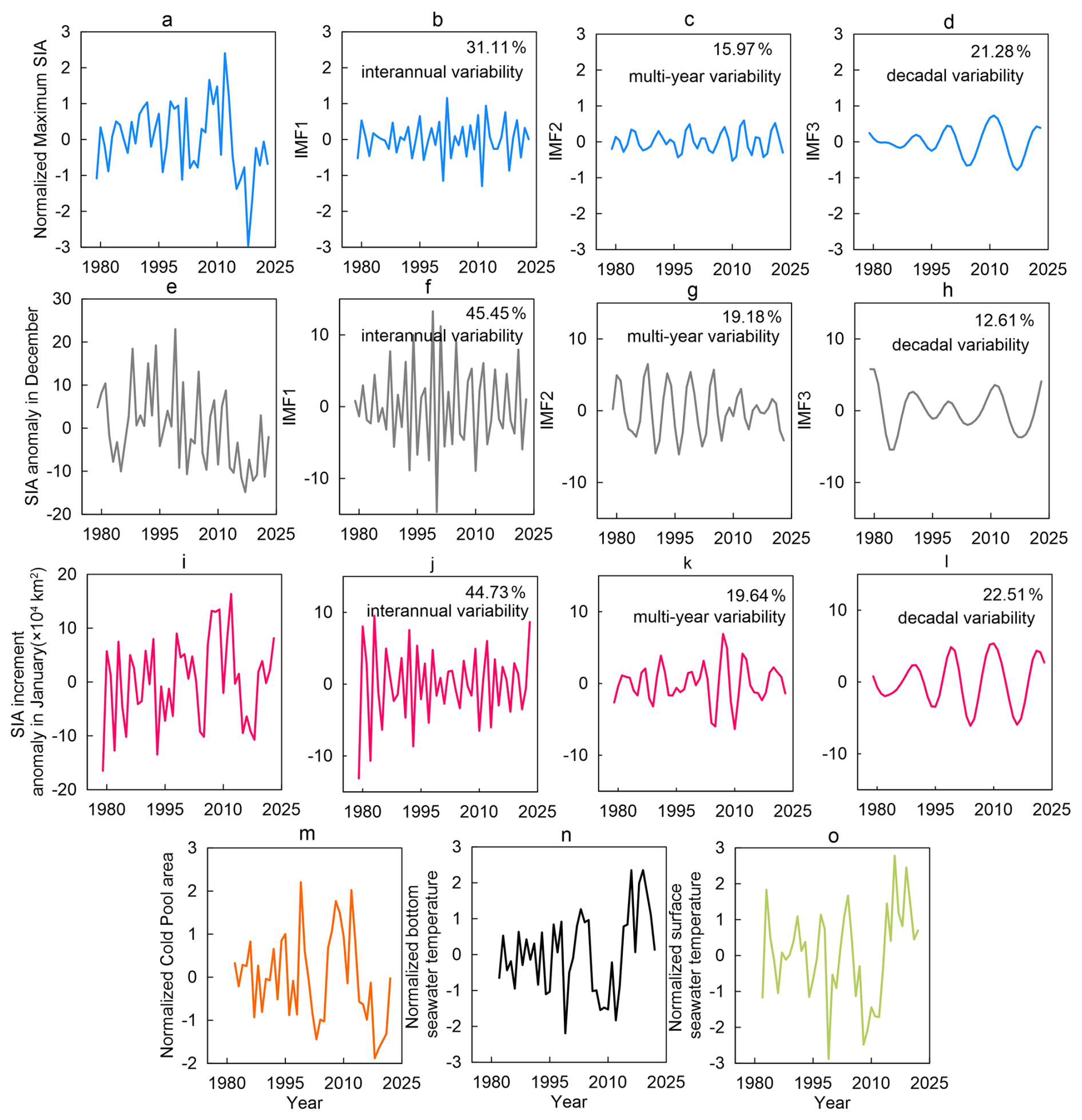
Figure 2 Time series of normalized maximum sea ice area (SIA; a), December SIA anomalies (e), and January SIA increment anomalies (ΔSIA; i) over the Bering Sea for the period 1979–2023, alongside their corresponding first three Intrinsic Mode Functions (IMFs; panels b–d, f–h, and j–l, respectively). Panels (m)–(o) present the time series of normalized spring cold pool area (m), normalized spring bottom seawater temperature (n), and normalized spring surface seawater temperature (o) for 1981–2022.

3 Results

3.1 Onset of timescale transition of SIA in Bering Sea

While several studies have definitively substantiated the timescale transition of sea ice from interannual to decadal variability in the Bering Sea (e.g. Wu and Chen, 2016; Yang et al., 2020) – a result corroborated by our calculations (Fig. 2a–d), attention has largely been restricted to the maximum sea ice extent. The specific onset month marking the emergence of these characteristics remains to be determined. We extracted the interannual, multi-year and decadal variability signals of SIA and ΔSIA from December to January. The analysis clearly indicates that December SIA (SIA₁₂) does not exhibit a transition from interannual to decadal variability (Fig. 2a–d). In contrast, the January ΔSIA is the first physical variable to demonstrate this shift (Fig. 2i–l), thereby inducing a corresponding transition in January SIA. This key finding is further supported by the ensemble empirical mode decomposition (EEMD) approach and Morlet wavelet analysis, which both reveal a pronounced intensification of the decadal signal in January ΔSIA over the past two decades. Detailed results are presented in Fig. S5 and Sect. S1, respectively. Such characteristics are not confined solely to sea ice; the spring mean surface and bottom seawater temperatures (Fig. 2m, n), as well as the Cold Pool Index (Fig. 2o) – defined as the area of the eastern Bering Sea shelf with bottom water temperatures below 2 °C during winter – also exhibit analogous transitional features. This implies the presence of a timescale transition within the integrated multi-layer system of the Bering Sea, extending beyond the domain of sea ice to encompass both the hydrological environment and the ecosystem. Consequently, subsequent analysis will prioritize the January ΔSIA.

Wang et al. (2022) employed EOF analysis to extract the leading two spatiotemporal modes of January ΔSIA (EOF1/PC1 and EOF2/PC2). Under positive PC1 conditions, EOF1 is characterized by pronounced sea ice reduction over the southern Bering Sea shelf. In contrast, positive PC2 corresponds to prominent sea ice increase over the northern Bering Sea shelf in EOF2. We note distinct temporal characteristics in the PCs of the first two leading modes: PC1 is dominated by multi-year variability, whereas PC2 exhibits prominent interannual variability (Fig. 4C, D in Wang et al., 2022). In the present study, we extracted the time series (PC1 and PC2) corresponding to these leading modes for the period 1979–2024. Utilizing the MODWT method, these series were decomposed into interannual, multi-year, and decadal components. For the subsequent analysis, the multi-year and decadal signals were aggregated, as illustrated in Fig. 3. Analysis reveals that PC1 primarily displays the multi-year and decadal variability (Fig. 3a), accounting for 55.2 % of the total energy, whereas PC2 is dominated by interannual variability (67.2 % of the total energy) (Fig. 3b). Notably, a comparative analysis reveals that EOF2 exhibits higher energy than EOF1 between 1983 and 2004 (Fig. 3c), signifying its dominance during this epoch, followed by a transition to EOF1 as the leading mode. This shift suggests that the temporal evolution of January ΔSIA from interannual to decadal variability is intricately linked to the transition in dominant spatial patterns from EOF2 to EOF1.

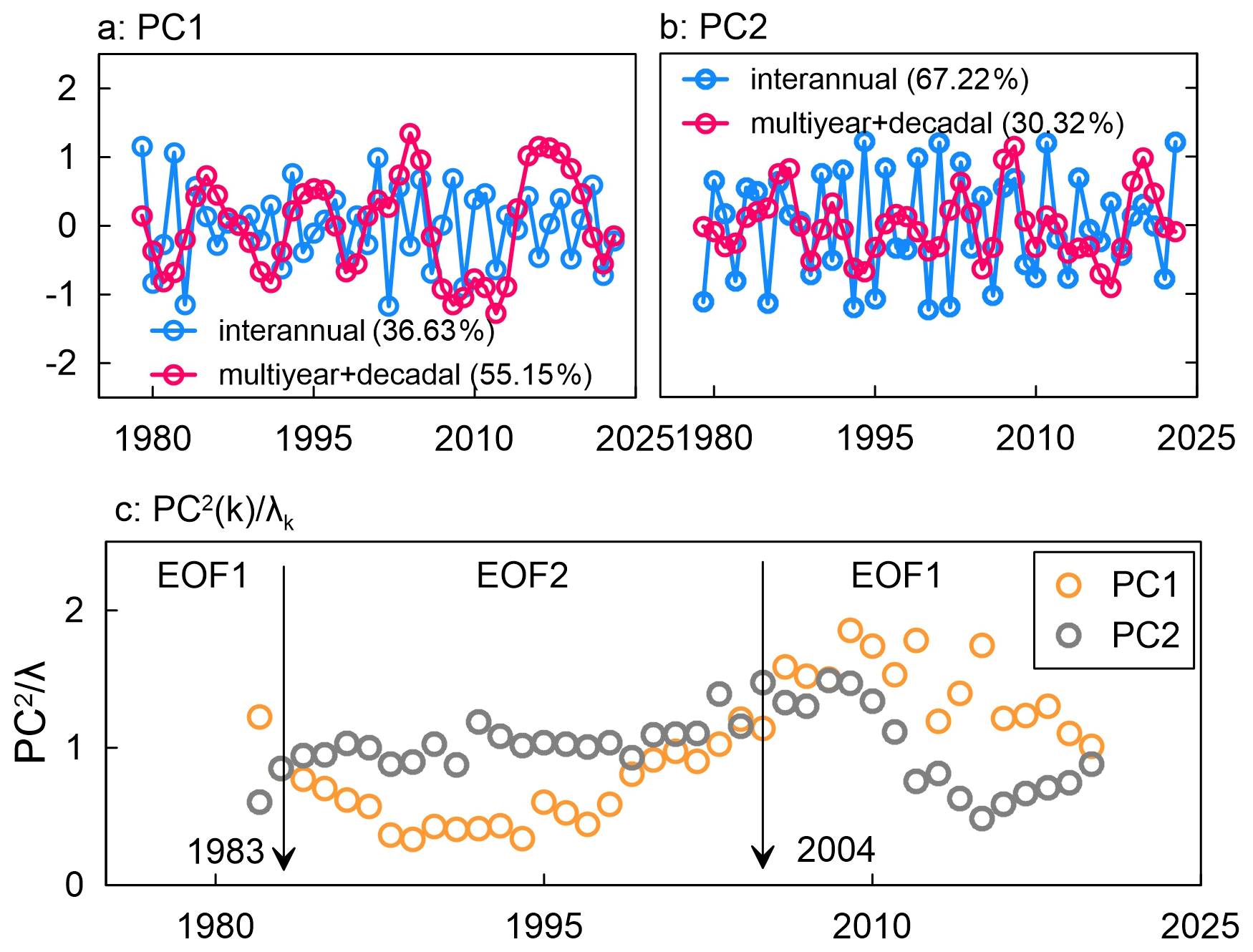
Figure 3 Multiscale variability of January sea ice area increment (ΔSIA) anomalies over the Bering Sea. Panels (a)–(b) present the multiscale variability of the principal component (PC) time series corresponding to the first two leading empirical orthogonal function (EOF) modes (EOF1 and EOF2), decomposed via maximal overlap discrete wavelet transform (MODWT) into interannual and combined multiyear-decadal components. Panel (c) shows the time series of variance-normalized squared principal components (${\text{PC}}^{\mathrm{2}}/\mathit{\lambda }$, where λ denotes the eigenvalue of the corresponding EOF mode) for PC1 and PC2. Vertical lines in panel c mark the years 1983 and 2004, critical transition points associated with a statistically significant regime shift in the spatial pattern of ΔSIA.

Therefore, a comprehensive understanding of the regulatory factors governing EOF1 and EOF2 is a prerequisite for elucidating the timescale transition of January ΔSIA in the Bering Sea. Prior research has explicitly established that EOF1 is primarily regulated by northward oceanic heat transport (Wang et al., 2022). Against this backdrop, the remaining inquiry focuses on two critical aspects: identifying the regulatory factors governing EOF2, and elucidating the mechanisms underlying the transition of dominant spatial patterns from EOF2 to EOF1. A comprehensive examination of the factors driving the observed shift in the dominant spatial patterns of January ΔSIA, and their associated physical mechanisms, will be presented in subsequent sections. Prior to delving into this analysis, however, it remains imperative to critically evaluate the influence of December SIA on January ΔSIA and determine whether a causal relationship exists between the two. This assessment serves as a foundation for the subsequent in-depth discussion of sea ice variability on the relevant timescales.

3.2 Impact of December SIA on January ΔSIA

We initially quantified the information flow from SIA₁₂ to January ΔSIA. The calculated $T_{{\mathrm{SIA}}_{\mathrm{12}}\to \mathrm{\Delta }\mathrm{SIA}}$ value was merely $-\mathrm{8.2}\times {\mathrm{10}}^{-\mathrm{5}}$, failing to reach the 95 % confidence level. Furthermore, the correlation coefficient between the two variables was calculated to be −0.02, which is statistically insignificant as well. However, SIA₁₂ exhibits a significant causal relationship with the leading principal components (PC1 and PC2) of January ΔSIA. The calculated information flows, $T_{{\mathrm{SIA}}_{\mathrm{12}}\to \mathrm{pc}\mathrm{1}}=-\mathrm{0.018}$ and $T_{{\mathrm{SIA}}_{\mathrm{12}}\to \mathrm{pc}\mathrm{2}}=-\mathrm{0.082}$, both achieve statistical significance at the 95 % confidence level. Moreover, a significant negative correlation between SIA₁₂ and PC1 becomes apparent after 2010 (Fig. 4b). Notably, the magnitude of this correlation increased markedly post-2015, reaching the 95 % confidence level. This suggests that the increase in SIA₁₂ may function as a precursor to enhanced SIA growth in the subsequent month. Additionally, PC2 exhibits a significant inverse relationship with SIA₁₂ prior to 2012. The correlation coefficient in Fig. 4c, approaching −1 during the 1990–2010 period, signifies that the increase in SIA₁₂ exerts a pronounced inhibitory effect on later SIA expansion.

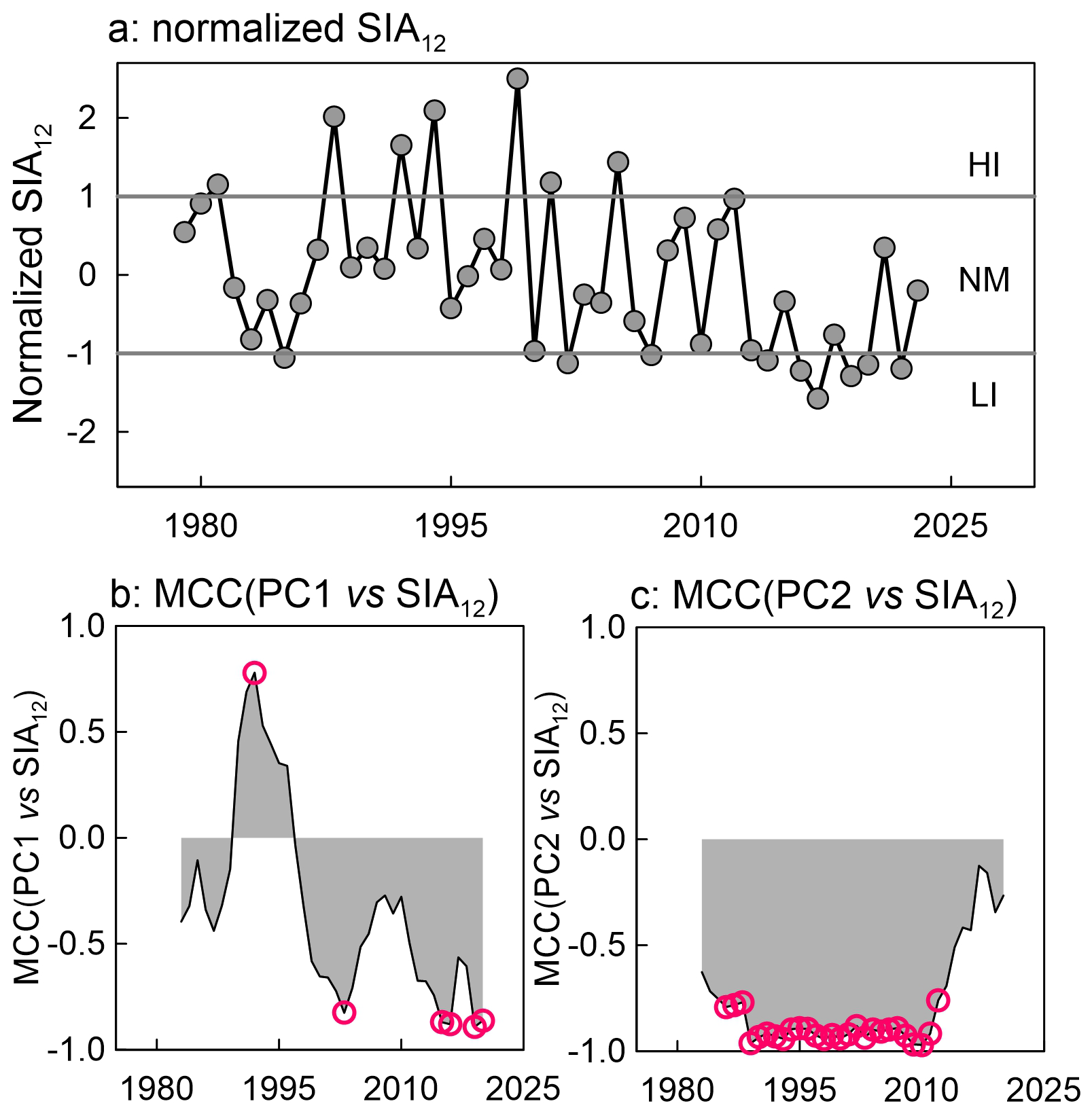
Figure 4 Statistical linkage between December sea ice area (SIA₁₂) anomalies and the principal components (PCs) of January sea ice area increment anomalies (ΔSIA) over the Bering Sea. (a) Normalized time series of December SIA anomalies, based on which the full observational record is stratified into three climatic regimes: heavy ice (HI) years, normal (NM) years, and light ice (LI) years. (b) Moving-window correlation coefficient (MCC) between PC1 and December SIA anomalies. (c) MCC between PC2 and December SIA anomalies. Red dots in all panels denote correlations that are statistically significant at the 95 % confidence level (p<0.05).

The negative information flow from SIA₁₂ to PC1 or PC2 suggests that the December sea ice area imposes a significant constraint on the January sea ice area in the following month. Furthermore, the co-occurrence of these two opposing effects of SIA₁₂ on subsequent ΔSIA (PC1 and PC2) implies the existence of distinct mechanistic pathways through which SIA₁₂ modulates the subsequent increment in SIA. One pathway displays noticeable interannual variability, whereas the other is associated with long-term decadal-scale changes. When the drivers promote the dominance of the EOF1 spatial pattern, SIA₁₂ contributes to fostering subsequent SIA, as exemplified by sea ice changes in the last two decades. Conversely, when EOF2-associated drivers prevail, SIA₁₂ impedes the sea ice expansion in later periods, as observed in the sea ice changes of the 1980s and 1990s. Crucially, regardless of whether EOF1 or EOF2 dominates, SIA₁₂ acts as a necessary precondition for initiating shifts in ΔSIA's spatial patterns.

Building on the preceding analyses, we hypothesize that December sea ice anomalies modulate the subsequent sea ice evolution via forcing perturbations to the overlying atmosphere and underlying ocean. The documented interannual-to-decadal transition in January ΔSIA emerges as a direct consequence of the competing influences of atmospheric versus oceanic forcing. To rigorously validate this hypothesis, we stratify the full observational record into three distinct regimes based on standardized SIA₁₂: light-ice (LI) years, heavy-ice (HI) years, and normal (NM) years. We subsequently employ composite analysis to quantify the forcing impacts of SIA₁₂ on the atmospheric and oceanic state.

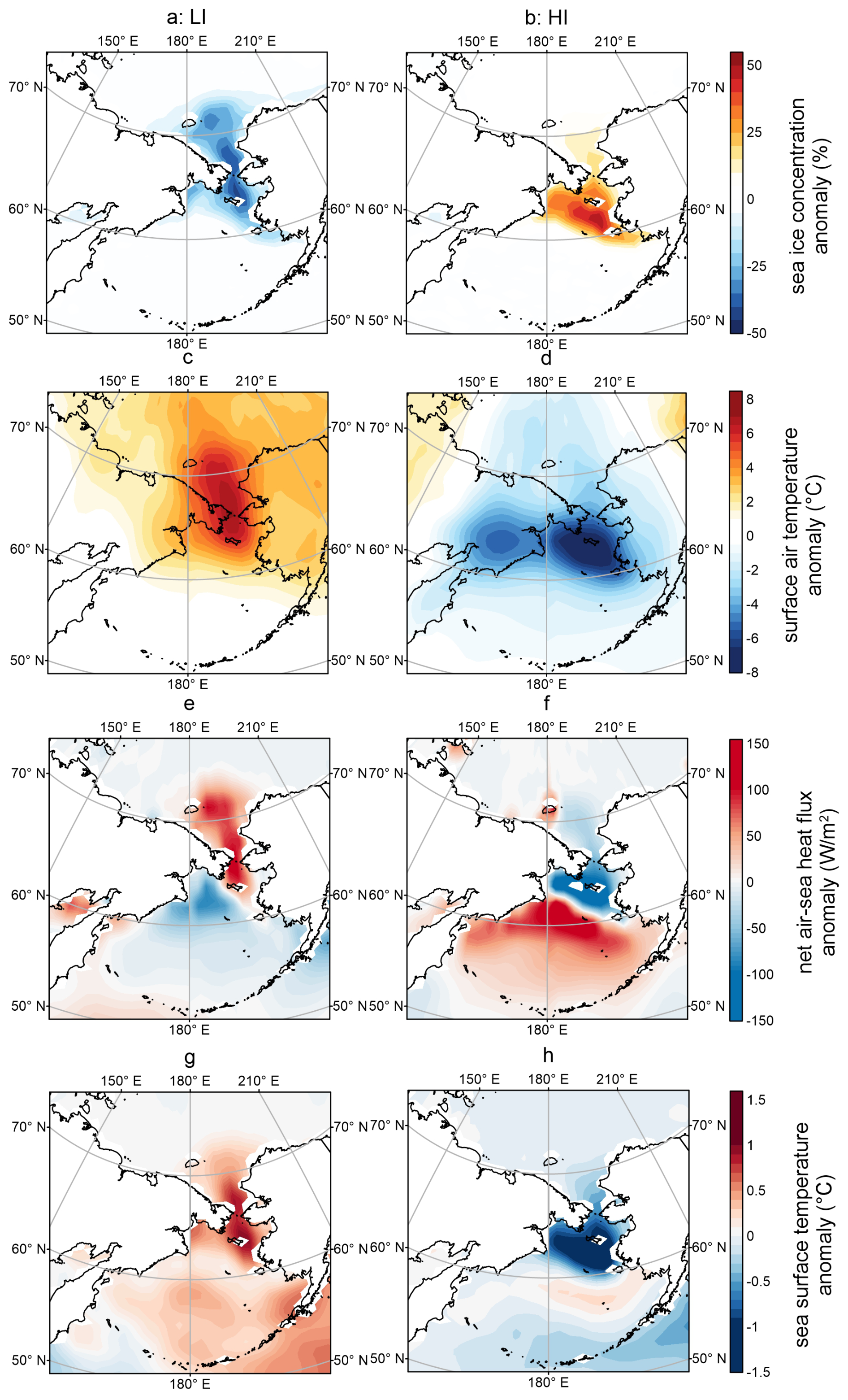
Figure 5 Composite anomalies of December sea ice concentration (SIC; a, b), surface air temperature (SAT; c, d), net air-sea heat flux (e, f), and sea surface temperature (SST; g, h) for light ice (LI) years (left panels: a, c, e, g) and heavy ice (HI) years (right panels: b, d, f, h), relative to the normal (NM) years.

3.3 Impact of the December SIA on the local net air-sea heat flux

Figure 5 presents the composite anomalies of December SIC, net air-sea heat flux, SST, and SAT for HI and LI years, relative to the NM years. During LI years, negative SIC anomalies are centred over the northern Bering Sea shelf, extending northward into the Chukchi Sea (Fig. 5a), with peak anomaly magnitudes approaching 0.4 %. Consistently, SST exhibits robust positive anomalies, reaching ∼1 °C in the waters surrounding St. Lawrence Island (Fig. 5g). The reduced sea ice cover and elevated SST drive a northward expansion of positive net air-sea heat flux anomalies (Fig. 5e), with local maxima exceeding +100 W m⁻². This enhanced ocean-to-atmosphere heat transfer in turn drives pronounced positive SAT anomalies, with local peaks as high as 6 °C (Fig. 5c). In contrast, during HI years, statistically significant positive SIC anomalies (Fig. 5b) and widespread negative SST anomalies (Fig. 5h) are concentrated over the northern Bering Sea shelf. This configuration drives marked negative anomalies in net air-sea heat flux, with a minimum of −150 W m⁻² around St. Lawrence Island (Fig. 5f). The strong insulating effect of the enhanced sea ice cover suppresses ocean-to-atmosphere heat exchange, resulting in SAT anomalies as low as −8 °C over the region (Fig. 5d).

Notably, the relationship between SIC anomaly and net air-sea heat flux is not strictly linear. We conducted a statistical analysis to explore the relationship between sea ice and air-sea heat flux in the Bering Sea, with detailed results presented in Sect. S2. Overall, in regions where sea ice exhibits obvious changes, the SIA₁₂ and net sea-air heat flux display an inverse correlation (Fig. 6a), indicating that reduced SIC₁₂ corresponds to enhanced upward net air-sea heat flux. The pronounced positive anomalies in net upward air-sea heat flux directly perturb the overlying local atmosphere, driving local atmospheric warming and amplifying ascending vertical motion (Fig. 6b). This dynamical atmospheric response, in turn, induces low-level horizontal mass convergence into the perturbed region (Fig. 6c). These dynamical features are fully consistent with the findings documented in Iida et al. (2020), who documented analogous ascending motion across the Bering-Chukchi Sea domain and mechanistically linked it to thermodynamic forcing driven by sea ice anomalies.

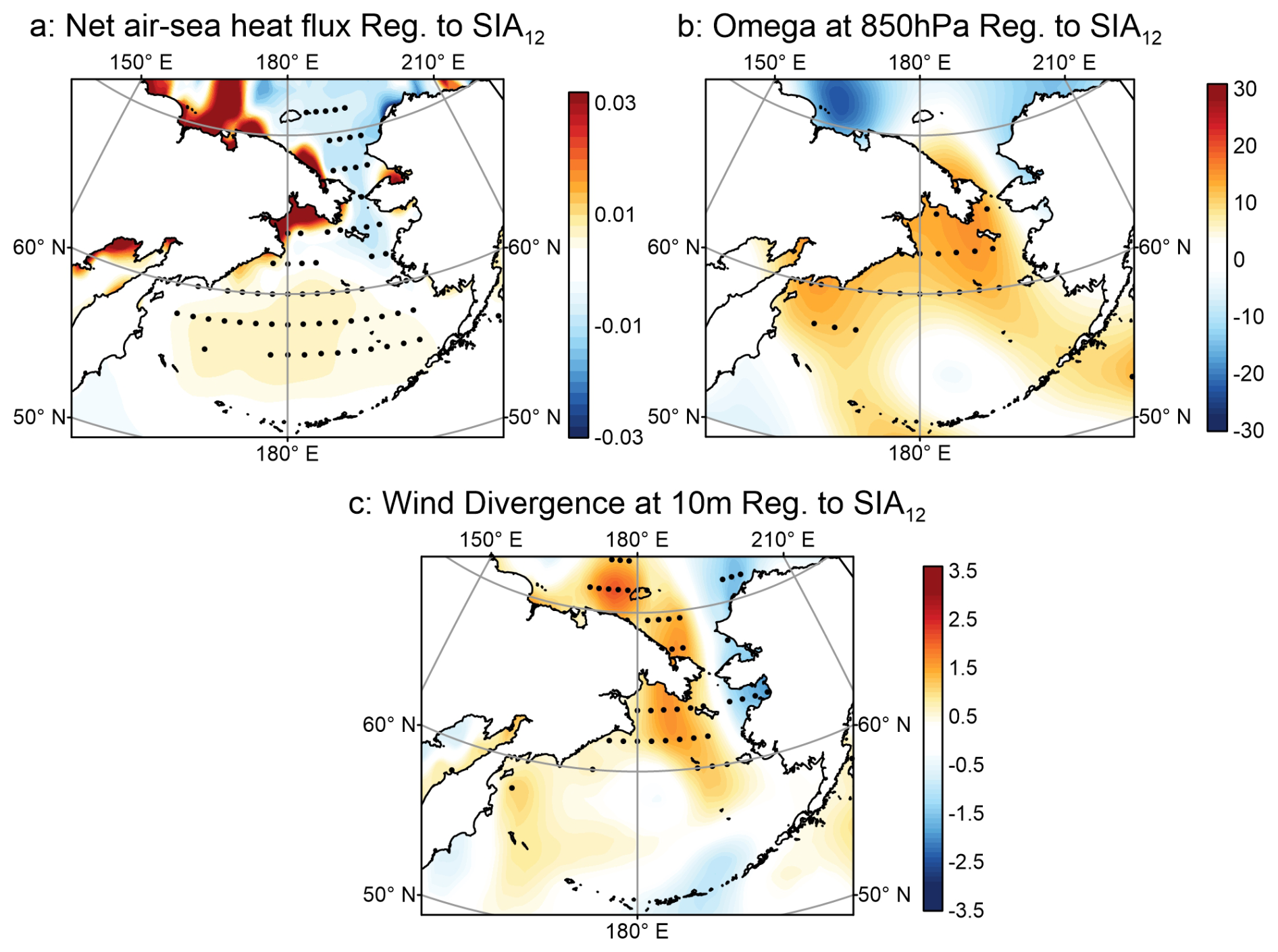
Figure 6 Regression maps of December variables over the Bering Sea regressed against normalized December sea ice area (SIA₁₂). Panels show: (a) net air–sea heat flux, (b) 850 hPa vertical velocity (Omega), and (c) 10 m horizontal wind divergence. Black dots in each panel mark statistically significant correlations (95 % confidence level, p<0.05).

3.4 Adjustment of wind field in December and its impact on the ΔSIA in January

Over the Bering Sea, the SLP is primarily modulated by two major semi-permanent atmospheric circulation systems: the Siberian High and the Aleutian Low (AL), which collectively govern the evolution of the regional climate system. Under the climatological mean state, the robust wintertime meridional SLP gradient amplifies geostrophic winds, with prevailing northeasterlies in the vicinity of St. Lawrence Island driving southward sea ice advection across the Bering Sea shelf (Fig. 7a). Marked spatial disparities in SLP anomalies emerge between LI and HI years, reflecting differential modulation of the large-scale circulation by preconditioning sea ice conditions. During LI years, a pronounced low-pressure anomaly dominates the southern Bering Sea, driven by extensive sea ice reduction that extends northward into the Chukchi Sea (Fig. 7c). Over regions with depleted sea ice cover, anomalous ascending air motion drives near-surface wind convergence (i.e., negative horizontal divergence anomalies). In stark contrast, HI years are characterized by a robust high-pressure anomaly centred over Siberia, whose influence extends eastward across the western Bering Sea shelf (Fig. 7e). This anomalous high-pressure system dominates the entire Bering Sea basin, with the associated anomalous wind divergence extending eastward across the northern shelf. Notably, this divergence anomaly is spatially collocated with positive SIC anomalies, implying a robust thermodynamic coupling between anomalous subsidence and enhanced sea ice cover. Despite the opposing SLP anomaly patterns between LI and HI years, their spatial structures are consistent with the third empirical orthogonal function mode (EOF3, Fig. 7h), which explains 14 % of the total variance in January SLP.

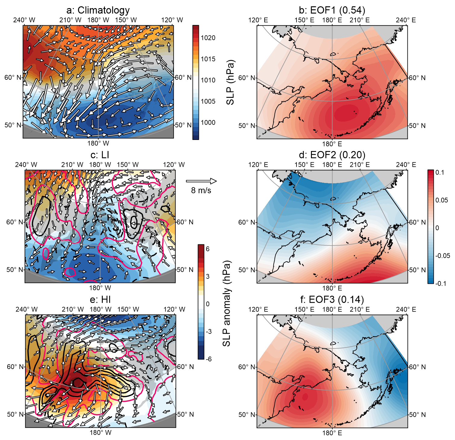
Figure 7 Response of the sea level pressure (SLP) and wind field to December sea ice area (SIA) anomalies over the Bering Sea. (a) Climatological mean SLP (color shading) and 10 m wind field (white arrows) for the study period. (c, e) Composite anomalies of SLP and 10 m wind vectors for light ice (LI) years (c) and heavy ice (HI) years (e), respectively. Contours denote wind divergence anomalies (units: $\times {\mathrm{10}}^{-\mathrm{5}}$ s⁻¹), with solid/dashed lines representing positive/negative anomalies, respectively, and the zero contour marked in red. (b, d, f) The first three leading EOF-decomposed spatial modes of December SLP, which explain 54 %, 20 %, and 14 % of the total variance, respectively.

Importantly, we emphasize that the basin-scale differences in SLP between HI and LI years are not driven by December SIA anomalies. Instead, these large-scale circulation discrepancies may be predominantly modulated by pan-Arctic climate variability and/or hemispheric-scale atmospheric dynamical processes. Our analysis focuses specifically on the mesoscale SLP variations over the northern Bering Sea shelf, which exhibit a robust out-of-phase spatial configuration between LI and HI events. Specifically, negative wind divergence anomalies extend northward into the Chukchi Sea during LI years, whereas positive wind divergence anomalies expand northward to the eastern Bering Sea coast during HI years. These mesoscale atmospheric perturbations can further drive the subsequent adjustment of sea ice conditions. Our statistical results reveal a statistically significant negative correlation between surface wind divergence over the waters south of St. Lawrence Island and the PC2 derived from EOF analysis of January ΔSIA anomalies (Fig. 8a). During LI years, the anomalous cyclonic circulation induced by ascending motion near St. Lawrence Island enhances sea ice divergence via wind forcing, which in turn leads to an increase in subsequent sea ice area. In stark contrast, the anomalous anticyclonic circulation driven by subsidence during HI years promotes sea ice convergence, ultimately resulting in a reduction of subsequent sea ice area.

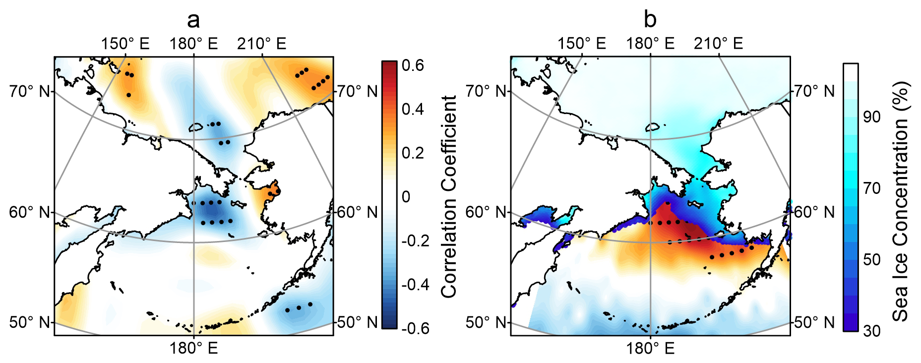
Figure 8 Linkages between January ΔSIA and coupled atmosphere-ocean processes over the Bering Sea. (a) Spatial correlation map between the PC2 derived from January ΔSIA and sea surface wind divergence for the period 1979–2023, with color shading representing the correlation coefficient. (b) Spatial correlation map between the PC1 derived from January ΔSIA and December northward heat transport over the same period, with color shading showing the climatological mean December SIC over the Bering Sea. Black dots in both panels denote correlations that are statistically significant at the 95 % confidence level (p<0.05). Both panels share an identical colorbar scale for correlation coefficients.

Additionally, the 10 m wind vector anomalies exhibit marked directional disparities between LI and HI years. During LI years, the dominant low-pressure anomaly drives southeasterly wind anomalies across the vicinity of St. Lawrence Island, enhancing northward Ekman heat advection. Conversely, HI events are characterized by a robust high-pressure anomaly that steers persistent westerly wind anomalies, suppressing cross-shelf northward meridional heat transport. This disparity in poleward heat transport directly modulates the subsequent evolution of sea ice cover, as corroborated by a strong positive correlation between northward heat transport and the PC1 of January ΔSIA anomalies over the southern waters of St. Lawrence Island (Fig. 8b). Notably, recent mechanistic analyses from Wang et al. (2022), based on mixed-layer heat budget diagnostics, have quantitatively demonstrated that December wind fields are the dominant driver of warm water transport variability over the northern Bering Sea shelf. Our study builds on this work to further quantify the impact of warm advection on sea ice, and clarifies the regulatory role of December sea ice on warm advection.

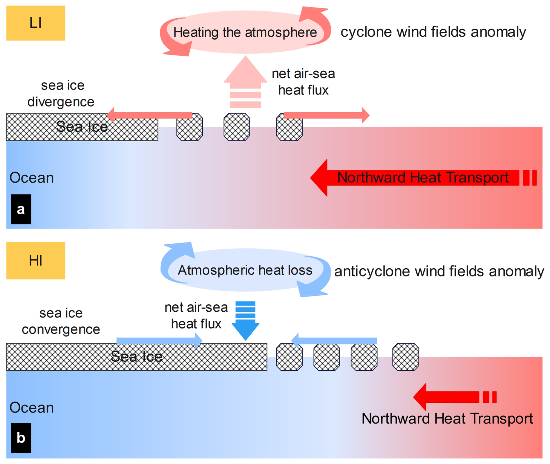
Figure 9 Mechanistic pathways of atmosphere-ice-ocean interactions driving SIA anomalies. In panel (a), a vertical-meridional view shows the process observed in LI years, wherein ascending air, induced by underlying warm sea water, causes a cyclone surface wind field anomaly. Consequently, poleward heat transport enhances, and the presence of cyclone wind field heightens the likelihood of sea ice expansion. Panel (b) displays a vertical meridional view in HI years, wherein extensive sea ice cover insulates air-sea heat exchange, inducing wind divergence that both facilitates sea ice accumulation and suppresses poleward heat transport.

Building on the foregoing analyses, we identify two distinct mechanistic pathways through which December SIA anomalies modulate the subsequent January ΔSIA over the Bering Sea, as synthesized in Fig. 9. First, an atmosphere-mediated thermodynamic negative feedback pathway: positive (negative) December SIA anomalies drive enhanced (reduced) surface wind divergence, which suppresses (promotes) SIA growth in the subsequent month. The spatial pattern of ΔSIA generated by this pathway aligns closely with the EOF2 mode of January ΔSIA, confirming that atmospheric thermodynamic forcing is the dominant driver of interannual variability in January ΔSIA. Second, an ocean-mediated dynamical positive feedback pathway: positive (negative) December SIA anomalies induce anomalous anticyclonic (cyclonic) surface wind circulation over the northern Bering Sea shelf. These wind anomalies in turn inhibit (facilitate) cross-shelf northward ocean heat transport, thereby enhancing (limiting) subsequent SIA growth. This mechanism corresponds to the leading EOF mode of January ΔSIA, and captures the decadal-scale variability of the regional sea ice system.

4 Discussions

4.1 Coupling of SIA anomalies and wind fields in December

Conventional understanding posits that only basin-scale SIA anomalies can drive statistically significant SLP responses (Vihma, 2014). However, the sea ice variability examined in this study is predominantly concentrated over the northern Bering Sea shelf, and the forcing effect of such mesoscale sea ice anomalies on local SLP, along with their underlying causal linkages, remains to be rigorously verified via targeted statistical causality tests. To systematically quantify the causal linkages between December SIA and atmospheric dynamics, we employed two complementary approaches: the Liang-Kleeman information flow analysis and the PAMIP multi-model ensemble simulations. Through Liang-Kleeman information flow analysis applied to SIA₁₂ time series and the first three spatial patterns of SLP anomaly in December, we detected no statistically significant causal information flow from SIA₁₂ to PC1 ($T_{{\mathrm{SIA}}_{\mathrm{12}}\to \mathrm{PC}\mathrm{1}}=\mathrm{0.0043}$) or PC2 ($T_{{\mathrm{SIA}}_{\mathrm{12}}\to \mathrm{PC}\mathrm{2}}=\mathrm{0.0013}$), with both values failing to meet the 95 % confidence threshold for statistical significance. In contrast, a robust, statistically significant information flow is identified from SIA₁₂ to PC3 ($T_{{\mathrm{SIA}}_{\mathrm{12}}\to \mathrm{PC}\mathrm{3}}=\mathrm{0.0093}$), which exceeds the 95 % confidence threshold. This result demonstrates a definitive causal influence of SIA₁₂ on the SLP spatial pattern captured by EOF3, highlighting the potential importance of SIA₁₂ in shaping the SLP captured by EOF3. This selective causality highlights the limited capacity of SIA₁₂ to modulate basin-scale December SLP.

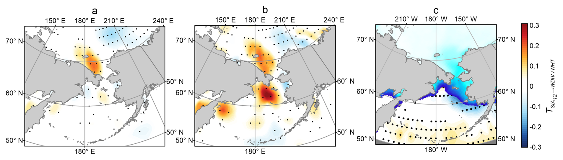
Figure 10 Liang-Kleeman information flows from SIA₁₂ to December wind divergence (a) and northern heat transport (c). Panel (b) exclusively focuses on the causal relationship between the two variables under HI and LI conditions. Black dots in both panels denote correlations that are statistically significant at the 95 % confidence level (p<0.05).

Of particular interest, Liang-Kleeman information flow analysis identifies a statistically significant positive causal link between SIA₁₂ and wind divergence around St. Lawrence Island (Fig. 10a, 95 % confidence level). During heavy/light ice (HI/LI) events, the information flow magnitude exceeds 0.2, indicating a robust causal linkage (Fig. 10b). This result demonstrates that SIA₁₂ variability influences the regional atmosphere via wind field modifications: while SIA₁₂ anomalies do not dominate basin-scale SLP patterns, they modulate mesoscale wind anomalies by altering local air-sea turbulent heat flux exchange. These wind adjustments play a critical intermediary role in regulating subsequent sea ice changes over the Bering Sea shelf in the following month.

The influence of wind fields on sea ice manifests not only through wind divergence but also via its modulation of NHT. We computed the Liang–Kleeman information flow from December SIA to NHT. Along the sea ice edge, the information flow metric $T_{{\mathrm{SIA}}_{\mathrm{12}}\to \mathrm{NHT}}$ exhibits significantly negative values, indicating that SIA₁₂ exerts a constraining influence on NHT variability. Notably, this negative value approaches −0.1, with a smaller magnitude than $T_{{\mathrm{SIA}}_{\mathrm{12}}\to \mathrm{WDIV}}$, which may arise from the modulating effect of SST and sea surface height on northward heat transport. Indeed, Wang et al. (2022) demonstrated using Reynolds decomposition that wind fields and SST contribute comparably to the variability of NHT.

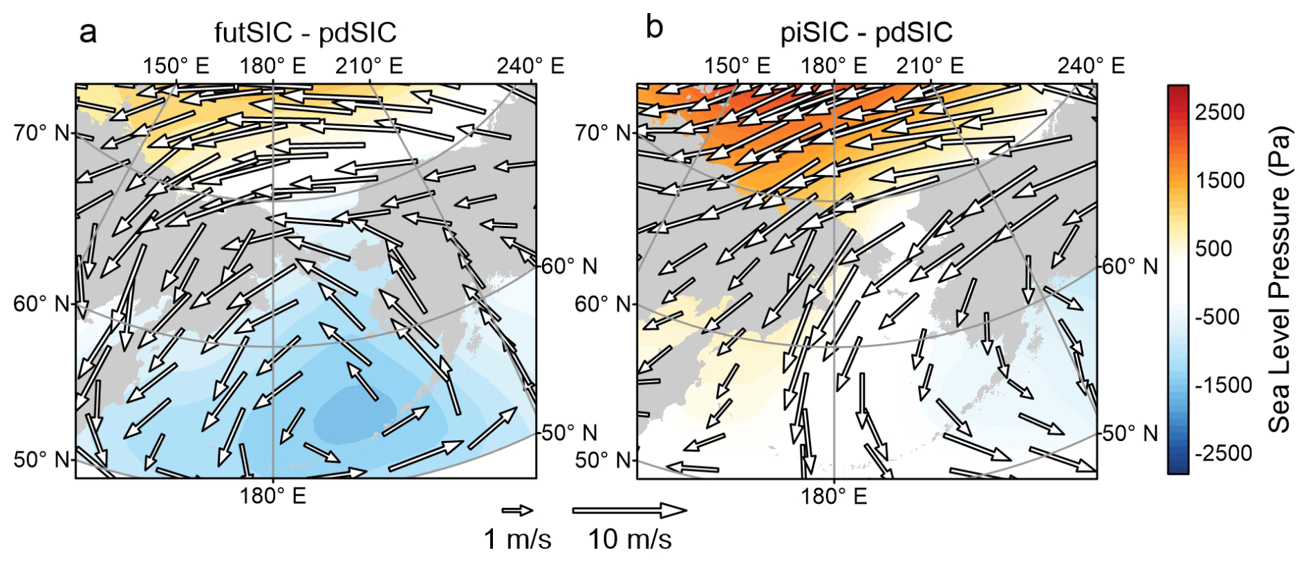
Figure 11 Composite differences of sea level pressure (SLP, colour shading, unit: Pa) and surface wind vectors (arrows, unit: m s⁻¹) derived from CESM2 simulations under contrasting sea ice concentration (SIC) forcing scenarios. Panel (a) quantifies the SLP and wind vectors differences between future (futSIC) and present-day (pdSIC) forcings, whereas panel (b) contrasts pre-industrial (piSIC) and pdSIC conditions.

The PAMIP simulations further corroborate the pronounced differences in atmospheric circulation responses to contrasting sea ice forcing conditions, with key results quantified in Fig. 11. Under December LI forcing, regions with extreme negative SIC anomalies are associated with anomalous low-pressure systems over the southern Bering Sea (Fig. 11a), collocated with a robust cyclonic circulation anomaly. This circulation pattern enhances both sea ice divergence over the northern shelf and poleward thermal advection along the northern flank of the cyclonic winds, which collectively suppresses equatorward sea ice expansion. Conversely, under extreme December HI forcing, a strong anticyclonic anomaly only appears substantial north of the Bering Strait towards the East Siberian Sea (Fig. 11b), driving widespread near-surface wind convergence. This wind field drives two competing dynamical effects: on the one hand, it promotes sea ice convergence, which acts to reduce total sea ice area; on the other hand, it suppresses cross-shelf northward ocean heat transport, which favours sea ice growth and expansion. While non-negligible spatial discrepancies exist between the simulated and observed SLP anomalies – most notably the more poleward (northward) displacement of the anticyclonic high-pressure anomalies under HI forcing – both the model simulations and reanalysis datasets consistently demonstrate a robust coupling between December mesoscale atmospheric processes and extreme SIA variability in the vicinity of St. Lawrence Island.

Rodionov et al. (2007) confirmed that the intensity and position of the AL consistently serve as significant proxies for pan-Arctic wind field variability and associated environmental shifts in the Northern Hemisphere. AL variability is tightly coupled to upper-tropospheric teleconnection patterns (Overland et al., 1999; Trenberth and Hurrell, 1994), particularly strong covariability between interannual AL intensity and the Pacific-North American (PNA) pattern (Lin et al., 2023; Sugimoto and Hanawa, 2009). Among known teleconnections, the Western Pacific (WP) pattern exhibits the strongest diagnostic capability for meridional AL displacements (Sugimoto and Hanawa, 2009; Wallace and Gutzler, 1981). Furthermore, the Arctic Oscillation and El Niño Southern Oscillation also modulate AL's position and intensity (Gong et al., 2017; Trenberth and Hurrell, 1994). It is crucial to highlight that the impact of mesoscale sea ice changes on wind field identified here represent fine-scale structural perturbations within the AL, rather than modifications to the large-scale AL system. Whether these localized mesoscale perturbations can alter the latitudinal displacement and intensity of the basin-scale AL remains an open question requiring targeted, in-depth investigation.

Additionally, compared with the results of previous studies (Danielson et al., 2011; Iida et al., 2020; Rodionov et al., 2007; Stabeno et al., 2012b; Wendler et al., 2014; Zhang et al., 2010), the spatial patterns identified in SLP during months extending beyond December identified in these prior works exhibit similarities to those characterized by the EOF3 derived from December SLP in this study. These earlier investigations proposed that the northeasterly wind anomalies associated with this SLP mode drive southward sea ice transport, resulting in basin-wide expansion of SIA. However, this long-standing conceptual framework is challenged by the lack of a statistically significant correlation between December near-surface wind speed and January ΔSIA anomalies, as documented in recent studies (Wang et al., 2022, 2024). Our findings further deviate from this established paradigm. We posit that this discrepancy with the traditional interpretation arises because the modulation of sea ice extent by the near-surface wind field is not governed by direct wind drag effects alone, but is instead dominated by sea ice convergence and divergence processes induced by wind drag forcing.

4.2 Competing mechanisms between atmospheric and oceanic forcing

Previous studies (Cheng et al., 2014; Li et al., 2014; Zhang et al., 2000, 2010) have consistently demonstrated that SIA variability in the Bering Sea is governed by the coupled interplay of thermodynamic and dynamic processes. Building on the comprehensive analysis presented herein, we identify the dominant drivers modulating the first two leading spatial modes of January ΔSIA in the Bering Sea as: (1) December northward heat transport along the sea ice edge (a core thermodynamic process), and (2) December near-surface wind divergence (a primary dynamic process). We therefore posit that the observed shift from interannual to decadal variability in January ΔSIA arises from the nonlinear competitive interplay between atmospheric and oceanic forcings. Notably, the impacts of these dual forcings on sea ice variability are modulated by the background state of the preceding December sea ice area (hereafter SIA₁₂). A rigorous, direct intercomparison of the relative magnitudes of these two forcings is therefore critical to accurately resolve the dynamics of their competitive interplay.

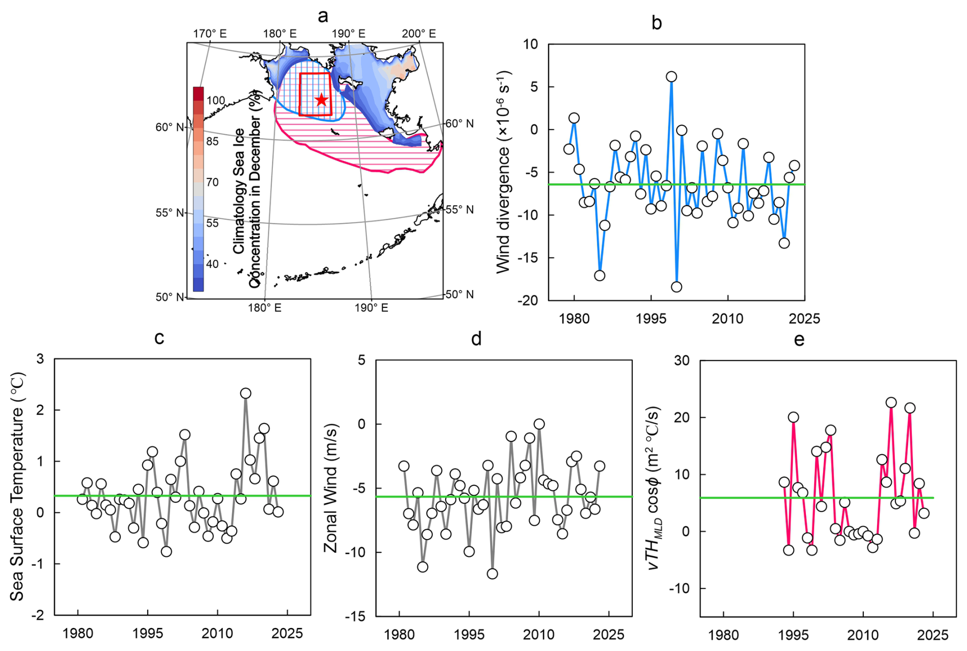
Figure 12 Time series of key ocean-atmosphere variables over the Bering Sea for the period 1979–2023. (a) Spatial map of the study domain, with the target analysis region (red rectangle) and its point (62.40° N, 174.20° W, marked by a red star); (b) near-surface local wind divergence; (c) December sea surface temperature (SST); (d) zonal wind; and (e) vTH_MLDcos ϕ. The green lines in panels (b)–(e) denote the long-term climatological mean of each corresponding variable across the full 1979–2023 study period.

As the northward heat transport is primarily governed by wind-driven Ekman transport, both driving factors – wind divergence and northward heat transport – share a common physical driver: the wind vector. Additionally, northward heat transport is modulated by SST. A detailed examination of the regions with significant correlation coefficients, as depicted in Fig. 8, identifies the southern Bering Sea shelf as the focal area where these driving factors exert the most pronounced effect on sea ice (Fig. 12a). Consequently, we extracted the time series of the local SST, zonal wind, wind divergence and northward heat transport (quantified as ϱ=vTH_MLDcos ϕ) from 1979 to 2023 within the shared region, as shown in Fig. 12. The observed SST (Fig. 12c) decreased markedly at a rate of −0.019 °C yr⁻¹ from 1979 to 1993, followed by a sustained increase of 0.016 °C yr⁻¹ after 1994. Concurrently, SST anomalies were muted prior to 1994 but exhibited pronounced large-amplitude variability thereafter. The near-surface zonal wind showed a post-1994 shift, with a prolonged positive anomaly during 2005–2014 and a sustained negative anomaly over 2015–2022. During 2016–2020, the mean SST anomaly reached 1.09 °C, and these large anomalies, coupled with persistent negative zonal wind anomalies, drove a sustained positive anomaly in northward oceanic heat transport. In contrast, wind divergence anomalies showed strong variability before 1994 but became substantially muted afterward, with only large-amplitude, episodic fluctuations in a small number of years.

From the EOF decomposition, the January sea ice area increment anomaly can be expressed as,

$$\mathrm{\Delta }\text{SIA}=\text{PC1}\times \text{EOF1}+\text{PC2}\times \text{EOF2}+\sum _{i=\mathrm{3}}^n\text{PCi}\times \text{EOFi}$$

This decomposition demonstrates that interannual variability in January ΔSIA anomalies is dominated when the PC2 exhibits enhanced deviations from its climatological mean. Correspondingly, decadal variability in ΔSIA emerges as the amplitude of the PC1 relative to its climatological mean increases. These inferences are consistent with the aforementioned variability in SST and wind divergence. Prior to 1994, wind divergence anomalies exhibited stronger amplitude fluctuations, whereas after 1994, northward heat transport anomalies displayed markedly larger amplitudes.

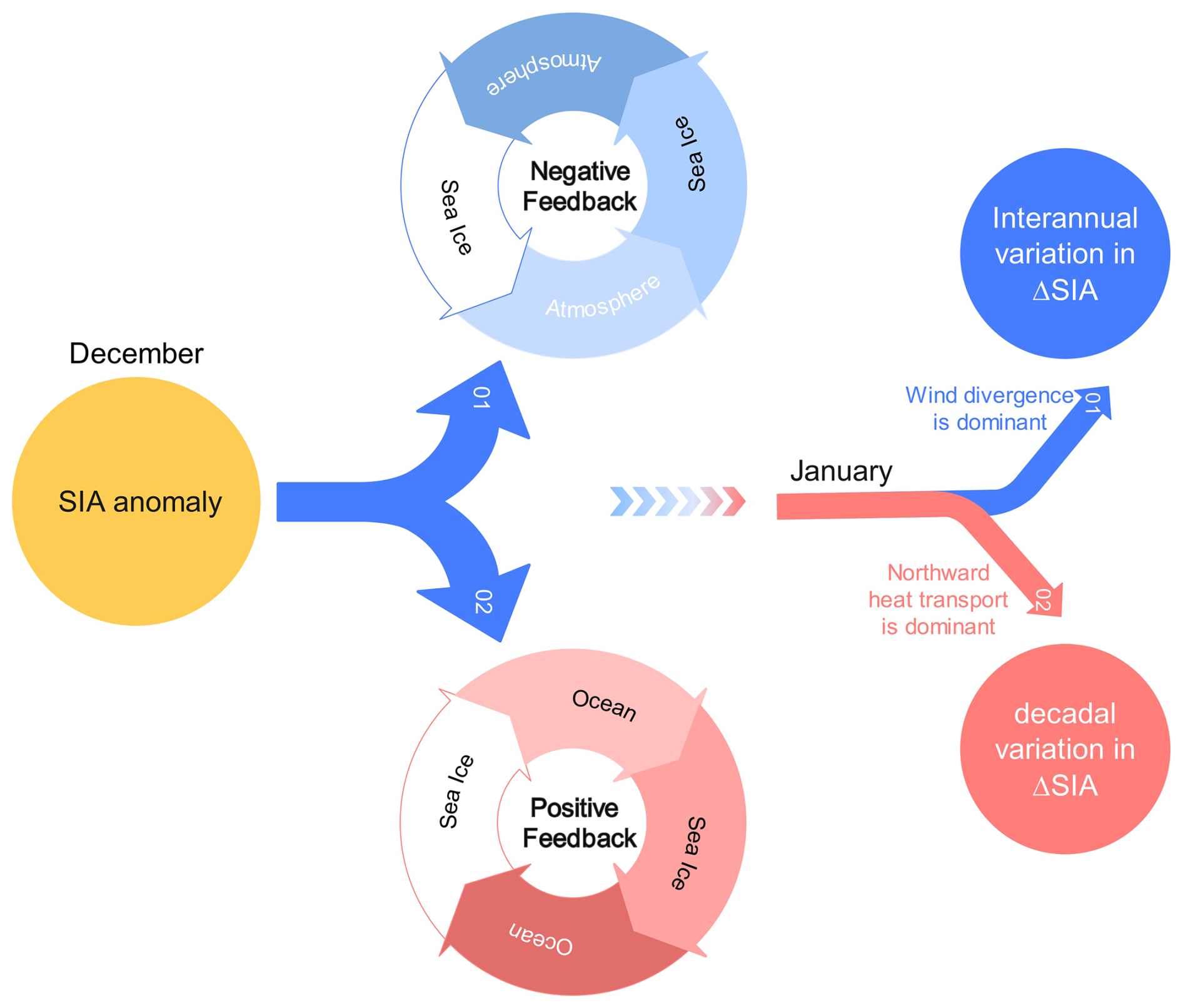
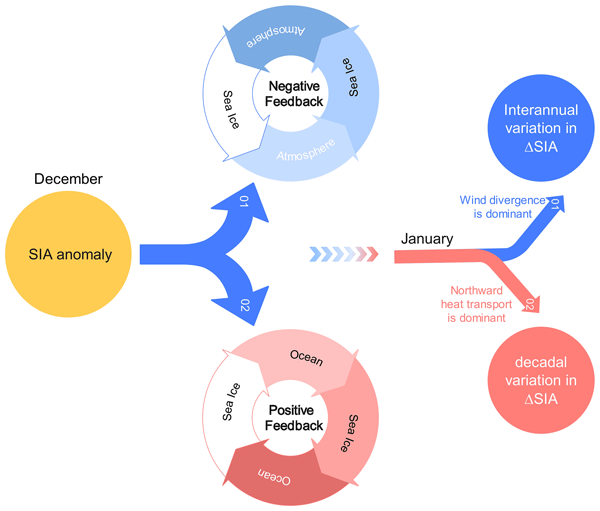
Figure 13 Schematic of the mechanistic processes driving the interannual-to-decadal timescale transition of SIA. December SIA anomaly triggers two feedback processes: oceanic feedback and atmospheric feedback. Oceanic feedback manifests as a positive feedback mechanism, inducing decadal fluctuations in ΔSIA. Conversely, negative feedback from the atmosphere yields interannual fluctuations in sea ice. The competition between wind field divergence and northward heat transport determining the fluctuation pattern of ΔSIA in January.

Figure 13 schematically illustrates the mechanistic framework governing the timescale transition of January ΔSIA. The process is initiated by preconditioning December SIA anomalies, which trigger two distinct and competing feedback mechanisms within the same month: (1) a positive feedback mediated by cross-shelf northward ocean heat transport, driving in-phase covariability between December SIA and subsequent January ΔSIA; and (2) a negative feedback governed by atmospheric thermodynamic forcing (i.e., wind divergence), generating out-of-phase changes in January ΔSIA. The temporal shift in the dominance of these two competing forcings directly determines the characteristic timescale of ΔSIA variability. During 1979–1994, when atmospheric forcing was the dominant control, ΔSIA exhibited predominantly interannual fluctuations. Since 1994, the growing influence of oceanic dynamical forcing has driven a transition to decadal-scale variability, which has persisted for nearly three decades.

Following 2018, a gradual recovery in December SIA has been observed over the Bering Sea (Fig. 2a). Concurrently, January ΔSIA anomalies have reverted to positive values, with the 2023 January ΔSIA reaching 2.7×10⁵ km² – the sixth highest value in the 45-year continuous satellite sea ice record. Associated with these shifts, the 2023 annual maximum SIA has approached the long-term climatological mean (Fig. 2e). Preliminary 2024 data reveal a continued recovery, with the annual maximum SIA reaching 5.1×10⁵ km², nearly indistinguishable from the climatological mean. Notably, this recent return to positive SIA anomalies emerges a decade on from the abrupt sea ice decline event in 2013, and thus merits close long-term monitoring to assess whether this shift signals a sustained reversal of the negative anomaly regime, and a potential persistence of positive SIA anomalies over the Bering Sea in the coming years.

Finally, we note that sea ice thickness was not included in the present analysis, owing to the scarcity of long-term observations and substantial uncertainties in satellite-based thickness retrievals across marginal ice zones. Sea ice acts as a thermal insulator between the ocean and atmosphere, with its thickness directly modulating the magnitude of air–sea heat fluxes. Sea ice convergence drives dynamic thickening, which dampens heat fluxes, suppresses ocean–atmosphere heat exchange, and promotes descending atmospheric motion, potentially accelerating the HI feedback loop in Fig. 9. However, the impact of sea ice thickness variations on air–sea heat exchange is likely considerably weaker than that driven by the presence or absence of sea ice itself, and the extent to which it modulates regional sea ice variability remains to be rigorously quantified via targeted in situ observations and process-based numerical simulations.

5 Conclusions

While atmospheric and oceanic forcings are well established as the primary drivers of sea ice variability in the Bering Sea, the specific mechanistic pathways and preconditioning triggers linking these forcings to sea ice changes remain poorly constrained. Critical knowledge gaps persist, particularly regarding the drivers of the well-documented regime shift in SIA temporal variability: the transition from interannual to decadal dominance since the mid-1990s. Here, we identify a pivotal, previously unreported observation: the earliest manifestation of this timescale transition in SIA variability occurs in the January ΔSIA anomaly. To explain this previously unresolved timescale shift, we propose a novel dual-feedback mechanism forced by coupled ocean-atmosphere responses to preconditioning December SIA anomalies. Specifically, December SIA anomalies trigger two competing, opposing feedback pathways within the same month: (1) a positive feedback mediated by cross-shelf northward ocean heat transport, which amplifies multi-year to decadal SIA variability; and (2) a negative feedback governed by near-surface wind divergence, which acts as the primary control on interannual sea ice fluctuations. Since 1994, the growing influence of oceanic heat transport in modulating Bering Sea SIA variability has strengthened this positive ice-ocean feedback loop. This regime shift explains the contemporary dominance of oceanic forcing in driving decadal-scale sea ice variability, supplanting the atmospheric drivers that prevailed during the late 20th century.

A key finding of this study is that the atmospheric circulation response to Bering Sea sea ice anomalies is predominantly localized to regions with the largest sea ice perturbations. While sea ice anomalies exert only a limited influence on basin-scale atmospheric circulation patterns, these localized circulation responses can drive substantial modifications to subsequent sea ice evolution, with the potential to trigger cascading atmospheric adjustments that modulate the broader mid-to-high latitude climate system. Consistent with recent work identifying a robust correlation between the PC1 of January ΔSIA and annual maximum SIA (Wang et al., 2022), our results highlight the critical role of early winter sea ice preconditioning in driving annual sea ice extremes. Future research should prioritize investigating this sea ice-driven causal chain to fully elucidate the tripartite interactions between sea ice, atmospheric circulation, and upper-ocean dynamics.

The ecological and biogeochemical consequences of prolonged heavy or light sea ice regimes in the Bering Sea are multifaceted, most notably the degradation and seasonal disappearance of the cold pool over the eastern Bering Sea shelf (Stabeno and Bell, 2019; Rohan et al., 2022; Belkin and Short, 2023), and the poleward shift of subarctic groundfish communities (Grebmeier et al., 2018; Rooper et al., 2021; O'Leary et al., 2022). Mirroring the shift in sea ice variability, the population dynamics of key Bering Sea ecological species have transitioned from interannual to decadal-scale fluctuations, with direct impacts on commercial and subsistence fishery yields. This regime shift poses profound adaptive challenges for indigenous communities and commercial fishing enterprises reliant on the stability and predictability of Bering Sea fishery resources. Under ongoing global warming, persistent upper-ocean warming in the Bering Sea means that sea ice cover is highly unlikely to revert to a predominantly interannual variability regime. Instead, the Bering Sea will likely remain prone to prolonged periods of heavy or light sea ice, locking in a shift in fishery resource fluctuations from interannual to decadal timescales. Consequently, fishery-dependent communities and management bodies must adapt to this new decadal-scale variability regime. While this shift offers greater multi-year predictability of sea ice and fishery conditions, it also presents substantial adaptive challenges associated with decade-scale shifts in fishery productivity and species distributions.