The anomalously warm summer of 2023 over Greenland as compared to previous record melt summers of 2012 and 2019

The Greenland ice sheet (GrIS) is a major regulator of Earth’s climate and sea levels. Atmospheric circulation anomalies have increasingly contributed to extreme summer melt events over the GrIS. Based on our analysis of the visible and near-infrared top-of-atmosphere reflectance (R^TOA), we identified the summer of 2023 as another such instance comparable to the anomalously warm conditions observed in 2012 and 2019. Individual summer month and combined June–July–August (JJA) R^TOA averages reveal that in 2023 the largest fraction of the GrIS experienced negative R^TOA anomalies exceeding one standard deviation below the 2007–2024 mean, including the high-albedo central ice sheet. By incorporating higher-level satellite retrievals, in situ automatic weather station data, reanalysis, and regional climate model output, we disentangle the R^TOA signal to better assess the processes that preconditioned and led to the observed negative R^TOA anomalies. We compare the extreme melt summers of 2012 and 2019 with 2023, to identify distinct pathways through which anticyclonic conditions contribute to GrIS surface melt. Our findings reveal that both clear-sky conditions, observed in 2019, and cloudy conditions, observed in 2012 and 2023, can trigger anomalous melting of the GrIS, with the primary difference being whether it is the margins or the central ice sheet that is most affected. Moreover, we find that both types of conditions are driven by atmospheric circulation patterns, shaped by the position, intensity, and persistence of anticyclones and the atmospheric rivers they help steer. Furthermore, were it not for the colder-than-average June in 2023, our findings show that the total summer melt would likely have rivaled the extreme levels observed in 2012.

1 Introduction

The Arctic is warming faster than the rest of the globe as a result of a set of positive feedback loops working in tandem. Among the most prominent of these feedbacks is the surface albedo feedback driven by sea ice and snow cover decline, as well as temperature feedbacks like those associated with the lapse-rate and the Planck response (Pithan and Mauritsen, 2014; Linke et al., 2023). This accelerated warming over the Arctic region is referred to as Arctic amplification (AA), and it has been studied for several decades (Manabe and Wetherald, 1975; Serreze and Barry, 2011; Pithan and Mauritsen, 2014; Wendisch et al., 2023). AA has been shown to directly contribute to the melt of the Greenland ice sheet (GrIS) (Colosio et al., 2021), which in turn drives global sea level rise (Mottram et al., 2019; Mouginot et al., 2019). The GrIS increasingly exhibits extreme melt events, which have become more frequent in recent decades due to anomalous atmospheric circulation patterns (Bennartz et al., 2013; McLeod and Mote, 2016; Blau et al., 2024). One of the most prominent of these melt events occurred on 11-12 of July, 2012, when more than 20 Gt of meltwater (Zheng et al., 2022) was generated as 98.6 % of the GrIS surface was undergoing melt (Nghiem et al., 2012) as a result of warm moist air advected from the North Atlantic. These wet air masses also promoted the formation of low-level liquid clouds which caused the surface to melt at higher elevations by enhancing the downwelling infrared radiative flux (Bennartz et al., 2013). The summer of 2012 set multiple records in terms of melt extent and duration, as well as near-surface temperature over the entire GrIS (Tedesco et al., 2013). Another such extreme melt event was on 31 July 2019 where ∼73 % of the ice sheet experienced surface melt, while the summer of 2019 set its own notable record of the largest negative surface mass balance (SMB) anomaly according to Modèle Atmosphérique Régionale (MAR) v3.10 simulations (Tedesco and Fettweis, 2020). Crucially, the principal causes behind these two major melt events differ in terms of air mass origin and temperature, cloudiness, snowfall and downwelling solar radiation at the surface (Tedesco and Fettweis, 2020; Hanna et al., 2021). Moreover, the pathway to these record melt summers is not always the same and most share only a few similarities, most common being the presence of high-pressure anticyclonic systems over the GrIS. In addition, the role of clouds during these episodes is not fully agreed upon, such that clouds are suspected to both contribute (Bennartz et al., 2013; Miller et al., 2015; Van Tricht et al., 2016) and limit (Hofer et al., 2017) melt across the GrIS. As such, this study conducts a spatiotemporal analysis of cloud and surface parameters during anomalously warm summers to better understand how future extreme melt events may affect the GrIS, the role of clouds in these events, and the methods available to monitor them.

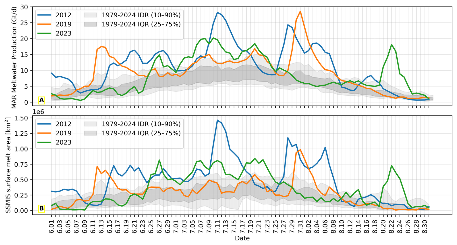
Figure 1 Plots of daily (A) meltwater production as simulated by the Modèle Atmosphérique Régionale and (B) SSMIS surface melt area for the summers of 2012 (blue), 2019 (orange), and 2023 (green). Interquartile and interdecile ranges are shown in dark and light gray, respectively.

Here, we examine the anomalously warm summer of 2023, a period which, to our knowledge, has not been studied as a distinct event. The summer of 2023, although it produced less melt than 2012 and 2019, had several noteworthy melt events spanning late-June to mid-July as well as a prominent multi-day episode in the second half of August (see Fig. 1). Consequently, we take 2023 as a case study and compare it to previous extreme melt summers. In doing so, we identify the causes and consequences of such extrema and address the similarities and differences between them. In particular, we take a look at the role of clouds and how their presence (or absence) contributes to melt and run-off during the anomalously warm summers of interest. Moreover, we investigate how the presence of clouds contributed to 2012 summer melt, how their absence contributed to 2019 summer melt, and what their role was during 2023 summer melt.

The main measured quantity we look at is visible-near infrared top-of-atmosphere reflectance (R^TOA) across the GrIS. Reflectance and derived parameters (e.g. albedo) are widely used to study the ice sheet; typically, studies apply atmospheric correction to RTOA to retrieve bottom-of-atmosphere reflectance (e.g. Casey et al., 2017) or derive broadband albedo (e.g. Stroeve et al., 2013; Shimada et al., 2016). Here, we adopt a distinct approach that avoids retrieval assumptions and their associated uncertainties, instead analyzing the raw satellite measurement. While R^TOA alone cannot disentangle the respective contributions of surface and clouds, its spatiotemporal analysis, paired with complementary higher-level satellite data products and model results, provides a more comprehensive framework for attribution (Lelli et al., 2023). For a full list of all the data utilized for this study, see Sect. 2. By examining monthly averaged RTOA without atmospheric correction or cloud masking, we observe the signal encompassing all modulating components, utilizing additional datasets to determine the drivers of these changes. This integrated approach offers greater confidence in the observed signals by leveraging both measurement and derived contextual information.

The three primary objectives addressed in this study are as follows:

1. To assess the effectiveness of R^TOA in the visible spectrum as a means to study the impact and severity of Greenland extreme melt summers.

2. To compare the anomalously warm summer of 2023 to that of 2012 and 2019, in order to better understand the different processes involved during such periods.

3. To assess the relationship between clouds and extreme melt events over the GrIS.

2 Data and Methods

We define $R_{\mathit{\lambda }}^{\mathrm{TOA}}$ for a given wavelength λ as in Lelli et al. (2023):

$$\begin{array}{}\text{(1)}& R_{\mathit{\lambda }}^{\mathrm{TOA}}={\displaystyle \frac{\mathit{\pi }{I}_{\mathit{\lambda }}}{\cos \left(\mathit{\theta }\right)E_{\mathit{\lambda }}^{\mathrm{0}}}}\end{array}$$

such that I_λ is the upwelling unpolarized spectral radiance at top of the atmosphere and $E_{\mathit{\lambda }}^{\mathrm{0}}$ is the unpolarized downwelling solar irradiance, where the 0 superscript denotes that it is measured outside the Earth's atmosphere and is therefore unattenuated. The angle θ denotes the solar zenith angle, i.e. angle between the sun and the local zenith at the point of observation.

2.1 Satellite-Based Measurements

We calculate $R_{\mathit{\lambda }}^{\mathrm{TOA}}$ from the measurement acquired by the Global Ozone Monitoring Experiment-2 (GOME-2), a scanning spectrometer carried by the polar-orbiting Meteorological Operational satellite (MetOp) series. Namely we use GOME-2A and B onboard the satellites MetOp-A and -B, respectively, which measure the Earth’s backscattered radiance as well as the extraterrestrial solar irradiance by means of a diffuser plate. In this way, the sun serves as a stable radiometric calibration source, which can be used to detect changes in the instrument’s sensitivity over time (Munro et al., 2016). All radiances measured at a solar zenith angle less than 90° are considered for calculating $R_{\mathit{\lambda }}^{\mathrm{TOA}}$. MetOp-A and -B were launched on 19 October 2006 and 24 April 2013, respectively, giving us a timeseries spanning the period 2007–2024 to work with. MetOp-A has since been decommissioned on 15 November 2021, but due to the tandem operations configuration of MetOp-A and -B, we seamlessly switch to GOME-2B after GOME-2A's swath width was reduced on 15 July 2013 (Munro et al., 2016). The choice of instrument is suitable given its spectral and spatial resolution as well as its Arctic coverage. For further details on GOME-2 instrument design and level 1 data processing, the reader is referred to Munro et al. (2016). For the purposes of this study, we derive I_λ and $E_{\mathit{\lambda }}^{\mathrm{0}}$ by averaging over spectral band 4 which encompasses visible and near-infrared wavelengths (576–790 nm). While band 3 (437–610 nm) includes a large part of the visible spectrum, band 4 better captures reflectance changes associated with extreme melt summers due to the higher absorption coefficient of ice and snow in the the red and near-infrared portion of the spectrum (Cooper et al., 2021). Consequently, all results shown in this study correspond to $R_{\mathit{\lambda }}^{\mathrm{TOA}}$ derived from Band 4, where λ= 576–790 nm.

To supplement GOME-2 $R_{\mathit{\lambda }}^{\mathrm{TOA}}$, we make use of the Energy Balanced and Filled (EBAF) top-of-atmosphere (TOA) data provided by the Clouds and the Earth’s Radiant Energy System (CERES) project (NASA/LARC/SD/ASDC, 2023). The EBAF-TOA dataset is derived from the CERES instruments that fly on the Terra, Aqua, Suomi National Polar-Orbiting Partnership, and National Oceanic and Atmospheric Administration (NOAA)-20 satellites (Loeb et al., 2018). In addition to radiation fluxes from the CERES instruments, the EBAF-TOA dataset also includes cloud properties derived from the Moderate Resolution Imaging Spectroradiometer (MODIS). The reader is referred to Loeb et al. (2018) for a full description of the EBAF-TOA dataset, the associated energy balance adjustments, and MODIS cloud data integration.

We also analyzed the GrIS surface melt extent record provided in the Greenland Ice Sheet Today (GIST) data collection (Mote, 2007, 2025). This dataset is derived from the Special Sensor Microwave/Imager (SSMI), and as of 2008 from the Special Sensor Microwave Imager/Sounder (SSMIS). It provides, daily, monthly (April–October), and annual melt areas (in km²) across the GrIS.

2.2 Ground-Based Measurements

To confirm anomalous behavior across the GrIS with in situ measurements we turn to the Greenland Climate Network (GC-Net) and Programme for Monitoring of the Greenland Ice Sheet (PROMICE) automatic weather station data. The PROMICE and GC-Net automatic weather station (AWS) dataset (How et al., 2025) is a combined initiative that brings together GC-Net AWSs operating since the 1990s and PROMICE which began in 2007. The combined dataset has a wide array of AWS covering the entire GrIS over both the accumulation (positive mass balance due to snowfall) and ablation (negative mass balance due to melt) zones (see Fig. 2). For more information on the methodology, AWS design, data processing, and a full list of all parameters measured, the reader is referred to Fausto et al. (2021). Lastly, here we also include data from the NOAA GEOSummit AWS measured at Summit Camp, available since installment in 2008 (Vandecrux et al., 2023).

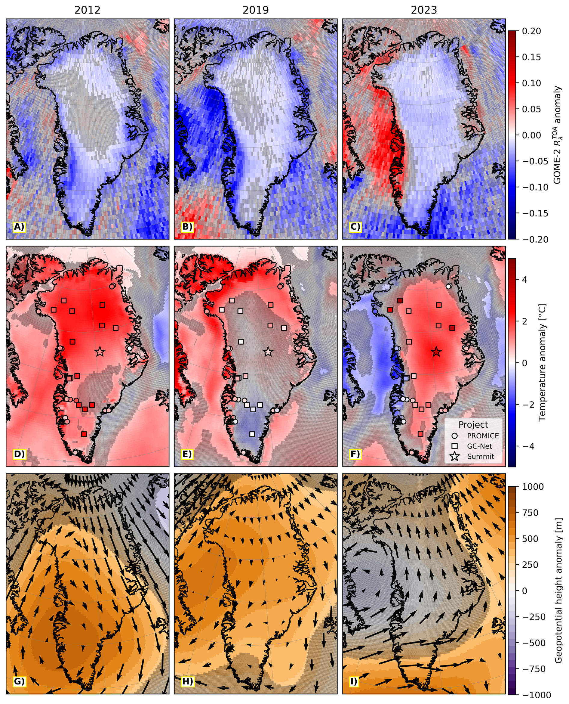
Figure 2 June–July–August (JJA) (A–C) GOME-2 reflectance at the top of the atmosphere ($R_{\mathit{\lambda }}^{\mathrm{TOA}}$) anomaly, (D–F) ERA5 2 m temperature anomaly along with PROMICE/GC-Net automatic weather station temperature anomaly at 2.7 m and Camp Summit anomaly at 2 m, and (G–I) ERA5 geopotential height anomaly at 500 hPa, where arrows represent wind anomaly at 500 hPa. The left, center and right columns correspond 2012, 2019 and 2023, respectively. All anomalies are calculated for the JJA of each year with respect the 2007–2024 JJA mean (individual automatic weather station mean values may cover a shorter timeframe based on the operational lifetime of each station). Grid cells without a gray filter are one standard deviation away from the mean.

2.3 Reanalysis

For parameters at selected heights and pressure levels, we make use of the fifth-generation global atmospheric reanalysis known as ERA5. Produced by European Centre for Medium-Range Weather Forecasts (ECMWF), ERA5 provides a wide range of variables at a horizontal resolution of 0.25°×0.25°, spanning 37 pressure levels and extending back to 1950 (Hersbach et al., 2020, 2023a, b). We choose ERA5 over other global atmospheric reanalysis data products as it is the most consistent and accurate at simulating atmospheric conditions over the GrIS (Chen et al., 2026). For the purpose of this study, we primarily make use of geopotential height and wind components at 500 hPa, 2 m temperature to compare with ground-based AWS data (see Fig. 2), and selected cloud properties (see Fig. 4). The geopotential height helps to quantify the presence and strength of high-pressure systems (blocking) over Greenland through the Greenland Blocking Index (GBI), which is typically defined as the mean 500 hPa geopotential height over the 60–80° N, 20–80° W region (Hanna et al., 2015; Tedesco and Fettweis, 2020). This index has been shown to be strongly linked with surface meltwater production across the GrIS (McLeod and Mote, 2016).

In addition to ERA5 data, we make use of the ERA5-based Dataset for Atmospheric River Analysis (EDARA) (Mo, 2024b, a) to also assess the influence of atmospheric rivers (ARs) during anomalous summers. Percentiles of parameters computed from ERA5 data, like integrated water vapor transport (IVT), are used as input for the Tracking Atmospheric Rivers Globally as Elongated Targets, version 3 (tARget-v3) algorithm developed by Guan and Waliser (2019). With this algorithm, a six hourly global AR dataset is created. To do so, tARget-v3 uses a combination of IVT geometry and intensity thresholds for AR identification. Contiguous IVT features exceeding an 85th-percentile threshold (with a minimum of 100 kg m⁻¹ s⁻¹) are selected and further constrained by poleward flow, directional coherence, minimum length, and length-to-width ratio criteria (Mo, 2024b).

2.4 MAR

For the analysis of SMB, melt and run-off during the summers of interest, we turn to the Modèle Atmosphérique Régionale regional climate model. MAR consists of an atmospheric module (Gallée and Schayes, 1994) coupled to the one-dimensional Soil Ice Snow Vegetation Atmosphere Transfer scheme (SISVAT) (Ridder and Gallée, 1998). Over the years MAR has been fine-tuned to polar environments by incorporating a snow-ice component into SISVAT based on Crocus (Brun et al., 1992), an energy balance model that determines the exchanges between ice, snow and atmosphere. MAR has a long history of having been utilized for simulations of the energy and SMB processes over the GrIS (Fettweis, 2007; Fettweis et al., 2011; Franco et al., 2012), with the simulated results having been validated through measurements (Lefebre et al., 2003; Fettweis et al., 2017). The model's physical parameterisations are calibrated to agree with the passive satellite derived melt extent (Fettweis et al., 2011). Since MAR is regularly updated, here we make use of the most recent version at the time of writing which is version 3.14.3. The reader is referred to Haacker et al. (2024) for an overview of the improvements introduced in MAR v3.14, and to (Grailet et al., 2025) for a detailed description of the ECMWF ecRad radiation scheme added in this version. For the purposes of this study, we make use of the 10 km horizontal resolution, aggregated daily data product forced by ERA5 reanalysis every 6 h at the lateral boundaries of MAR. For more information on how ERA5 is utilized to force MAR, as well as the evaluation of the results, the reader is referred to Delhasse et al. (2020).

3 Results

Figure 2A–C display $R_{\mathit{\lambda }}^{\mathrm{TOA}}$ anomalies, which are defined as the difference between the measured $R_{\mathit{\lambda }}^{\mathrm{TOA}}$ averaged over the month of June, July and August (JJA) of each year (2012, 2019, and 2023) and the 2007–2024 JJA mean. All three years show predominantly negative $R_{\mathit{\lambda }}^{\mathrm{TOA}}$ anomalies across the GrIS during these three months (see Fig. 2A–C), with strongly negative values along the southwestern margin in 2012 and 2019, and on the southern tip of the ice sheet in 2023. In this figure, as well as all anomaly maps from here on, the low opacity gray filter is used to designate anomalies that are within one standard deviation of the mean.

At the surface, we look at ERA5 2 m temperature anomalies overlaid with PROMICE, GC-Net and Summit Camp AWS ground-based measurements (see Fig. 2D–F). Because GC-Net AWS data is assimilated into ERA5, there is good agreement between the anomalies (Covi et al., 2025). Summit Camp and PROMICE AWS, on the other hand, are not assimilated into ERA5, thereby giving an independent assessment of the reanalysis (Fausto et al., 2021). In 2012, positive temperature anomalies span the entirety of Greenland, in 2019, they are primarily concentrated along the coast towards the Northern side of the island, and in 2023, they cover the central parts of the GrIS.

Figure 2G–I shows the geopotential height anomaly at 500 hPa with arrows representing the wind anomalies at that same pressure level. The Greenland-wide positive geopotential height anomaly in 2012 and 2019 show atmospheric ridges that were present for a significant portion of both summers. The 2023 JJA average, on the other hand, predominantly has its geopotential height anomalies within one standard deviation of the 2007–2024 JJA mean. While anticyclones were also present in 2023, a strong cyclone on the western coast of Greenland in June reduces the JJA geopotential height average. To disentangle seasonal variation and focus on one month in particular, we select July as it is typically when the GrIS melts the most within a given year.

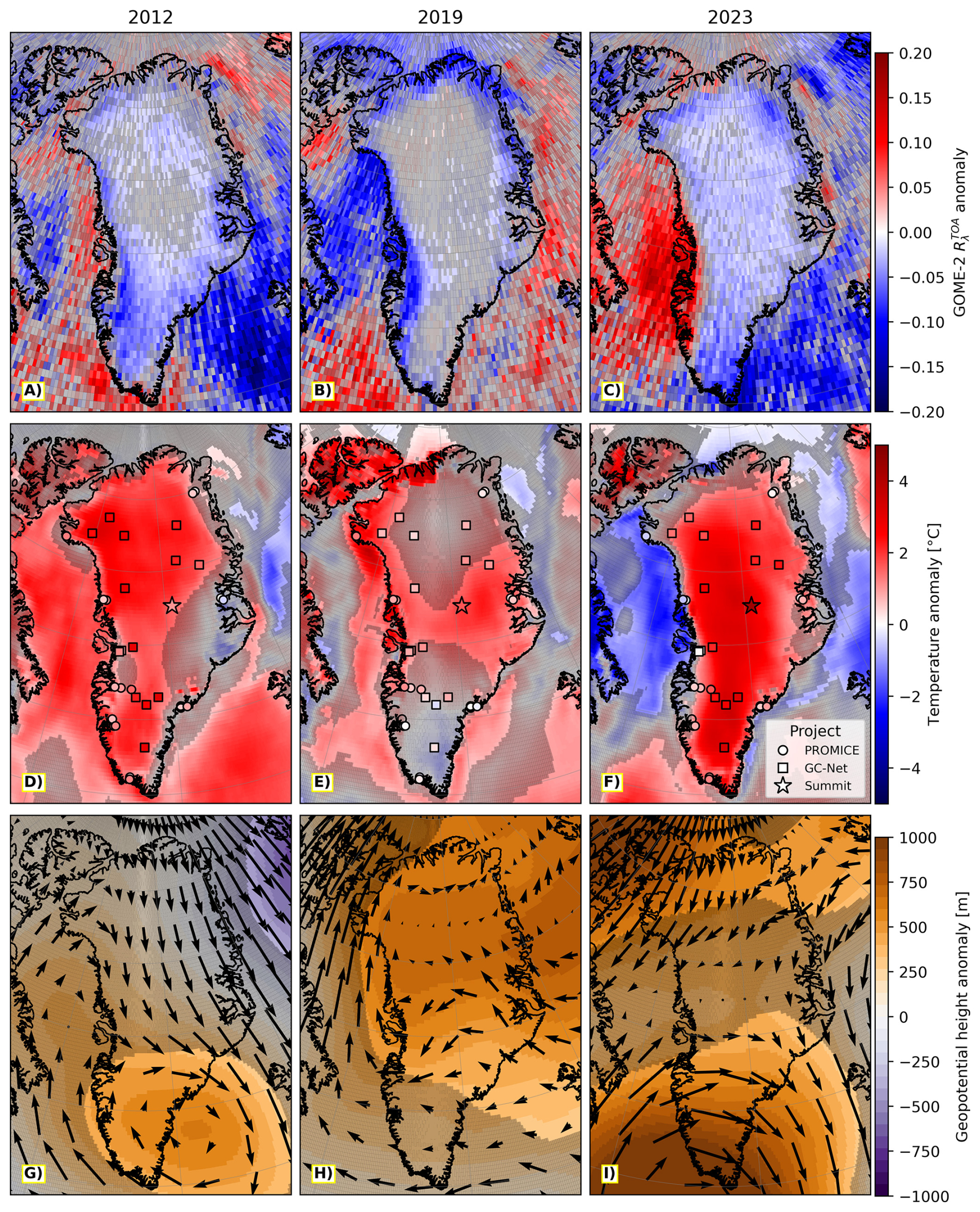
Figure 3 July (A–C) GOME-2 reflectance at the top of the atmosphere ($R_{\mathit{\lambda }}^{\mathrm{TOA}}$) anomaly, (D–F) ERA5 2 m temperature anomaly along with PROMICE/GC-Net automatic weather station temperature anomaly at 2.7 m and Camp Summit anomaly at 2 m, and (G–I) ERA5 geopotential height anomaly at 500 hPa, where arrows represent wind anomaly at 500 hPa. The left, center and right columns correspond 2012, 2019 and 2023, respectively. All anomalies are calculated for the July of each year with respect the 2007–2024 July mean (individual automatic weather station mean values may cover a shorter timeframe based on the operational lifetime of each station). Grid cells without a gray filter are one standard deviation away from the mean.

With 2012 breaking the melt record on 11 July (Zheng et al., 2022), 2019 reaching its maximum daily melt on July 31 (Tedesco and Fettweis, 2020), and 2023 having multiple melt episodes 6–22 July, all three Julys were exceptional as compared to the middle 80 % of 1979–2024 July melt data (see Fig. 1). In Fig. 3 the pronounced negative Greenland-wide $R_{\mathit{\lambda }}^{\mathrm{TOA}}$ anomaly can be seen in 2023, with high 2 m temperature anomalies (above 4 °C) concentrated along the central part of the GrIS. Looking at the geopotential height and wind anomalies (Fig. 3G–I), both 2012 and 2023 exhibit a strong anticyclone on the southern tip of the island directing air masses from the South onto the GrIS. Unlike 2012 and 2023, 2019 July $R_{\mathit{\lambda }}^{\mathrm{TOA}}$ negative anomaly is most pronounced around the margins of the GrIS.

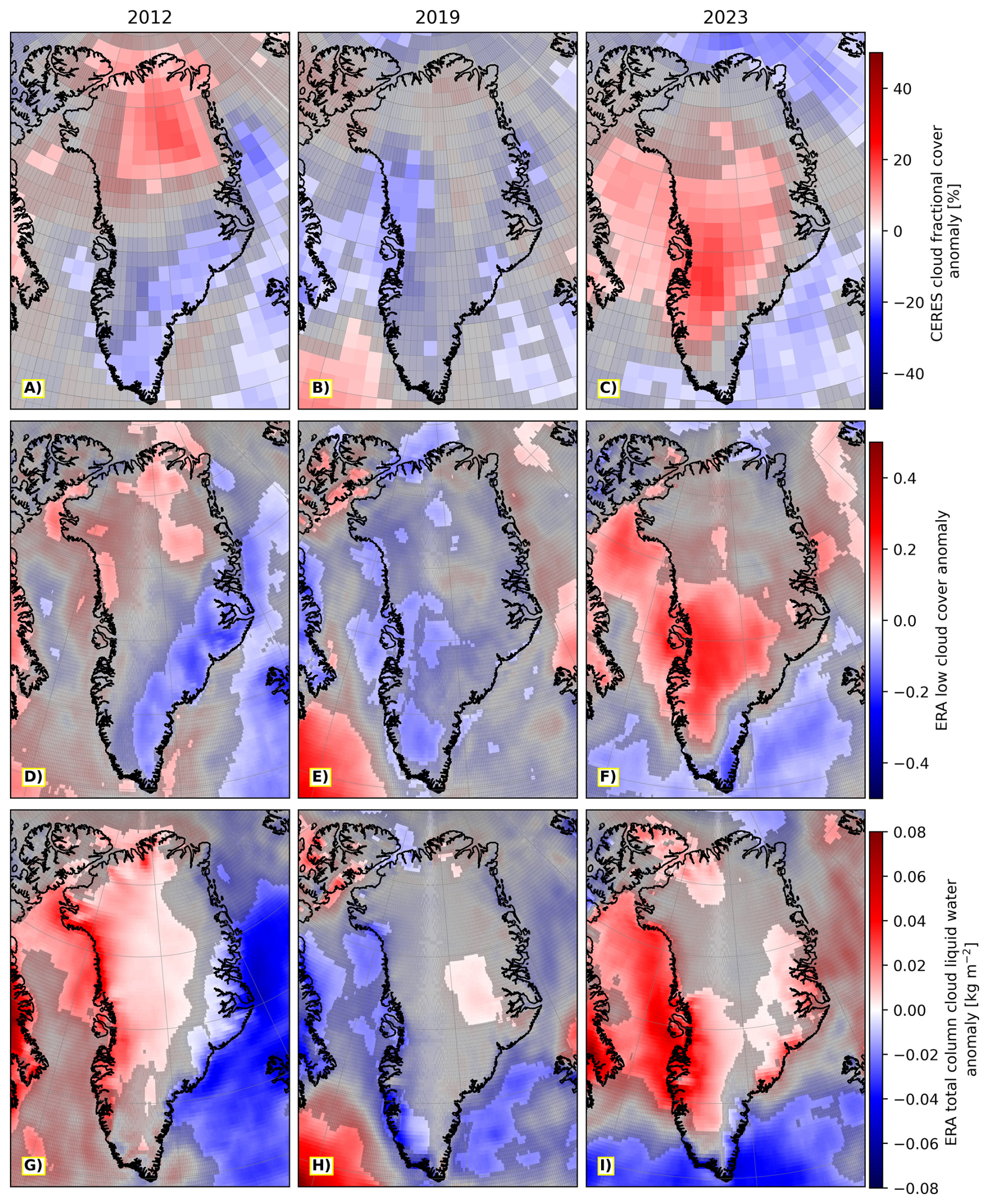
Figure 4 June–July–August (JJA) (A–C) CERES EBAF-TOA cloud cover anomaly, (D–F) ERA5 low cloud cover anomaly or clouds on model levels at ca. 800 hPa, (G–I) ERA5 total column cloud liquid water anomaly. The left, center and right columns correspond to 2012, 2019 and 2023, respectively. All anomalies JJA of each year with respect the 2007–2024 JJA mean. Grid cells without a gray filter are one standard deviation away from the mean.

To better dissect the $R_{\mathit{\lambda }}^{\mathrm{TOA}}$ anomaly distribution, cloud properties that affect reflectance in the visible/near-infrared spectral band must also be considered (Fig 4A–C). Anomalies computed the same way as for Fig. 2, but for cloud parameters, are shown in Fig. 4. The summer of 2012 and 2023 both show positive CERES cloud cover and ERA5 total column cloud liquid water (TCLW) anomalies (relative to the 2007–2024 average). Meanwhile, the summer 2019 average shows predominantly negative cloud cover anomalies throughout the island, as reported by Tedesco and Fettweis (2020). Delving into ERA5 low cloud cover anomalies or clouds occurring on model levels with a pressure greater than 0.8 times the surface pressure of ∼ 800 hPa (Fig. 4D–F), a strong low cloud cover anomaly can be seen on the Western coast of Greenland in the 2023 summer average.

Unlike with Figs 2 and 3, the differences in JJA and July cloud property average values across the GrIS are not as pronounced suggesting that July conditions heavily influenced the JJA average. To compare Fig. 4 against the averages from July, see Fig. A1 in Appendix A. Notable differences include the more pronounced negative cloud property anomalies in the Northern part of Greenland in July 2019, as well as a more pronounced anomaly (up to 0.08 kg m⁻²) of TCLW on the western coast in July 2023.

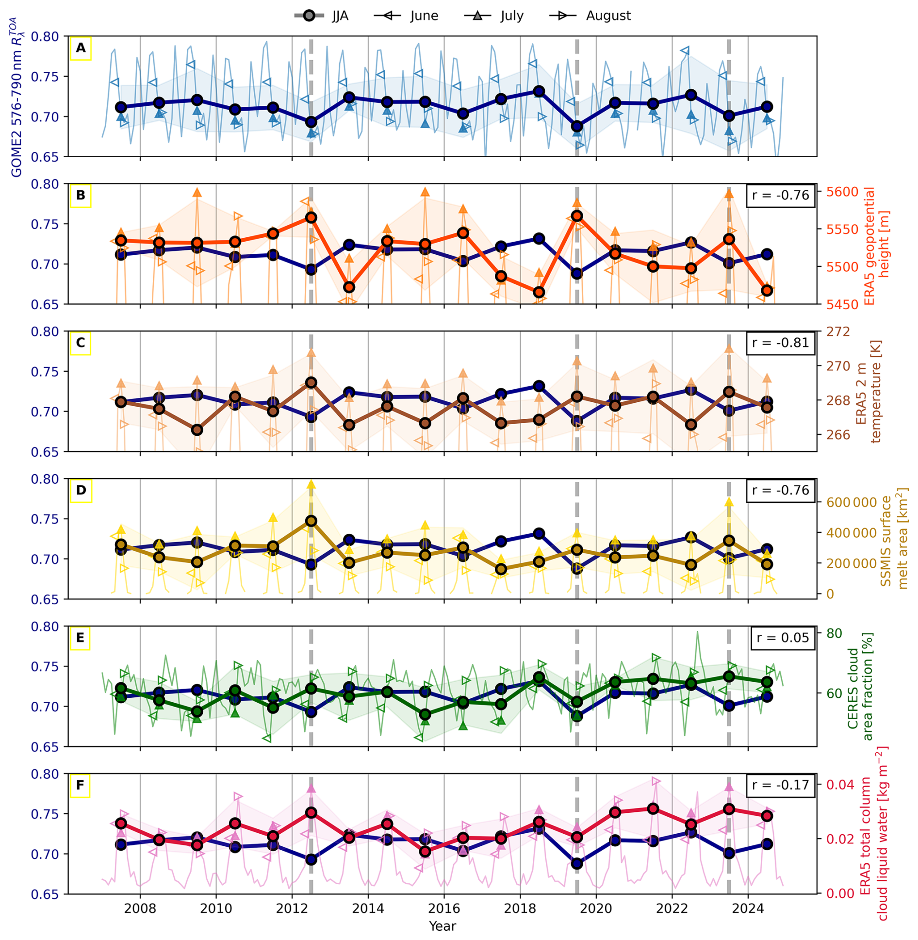
Figure 5 Time series of (A) GOME-2 reflectance at the top of the atmosphere ($R_{\mathit{\lambda }}^{\mathrm{TOA}}$) over Greenland, plotted alongside (B) ERA5 500 hPa Geopotential Height averaged over the 60–80° N, 20–80° W region, (C) ERA5 2 m temperature, (D) SSMIS surface melt area, (E) CERES cloud area fraction, and (F) ERA5 total column cloud liquid water, respectively. Filled circles connected by thick solid lines show only the June–July–August (JJA) averages, while the thinner line depicts the full monthly dataset. June, July and August means are all individually represented by left, up and right-facing triangels, respectively. All points in the time series represent Greenland-wide spatial averages weighted by latitude for the respective parameter. The data is color-coded according to the axis label, and the semi-transparent sleeves around the main data represents one standard deviation (calculated over the averaging period). Vertical dashed gray lines represent the anomalous summers of interest: 2012, 2019 and 2023. The pearson correlation coefficient reported in the legend is computed between the JJA averages of the parameters shown in each subplot.

To illustrate how other years relate to the selected ones, Fig. 5 depicts the time series of spatially averaged variables in question and confirms the findings shown in Figs. 2 and 4. All three anomalous summers of interest show a similar pattern of low $R_{\mathit{\lambda }}^{\mathrm{TOA}}$ and high averaged geopotential height in Fig. 5A. In addition, a Pearson correlation coefficient of −0.76 indicates that this opposing pattern between the two variables is present throughout the time series. $R_{\mathit{\lambda }}^{\mathrm{TOA}}$ has a similarly strong anticorelation of $r=-\mathrm{0.81}$ and $r=-\mathrm{0.76}$ with 2 m temperature and melt area extent, respectively (Fig. 5B–C). While Fig. 5A, B and C show a similar story, the summer of 2019 has a relatively high geopotential height average but low average 2 m temperature and surface melt area extent averages.

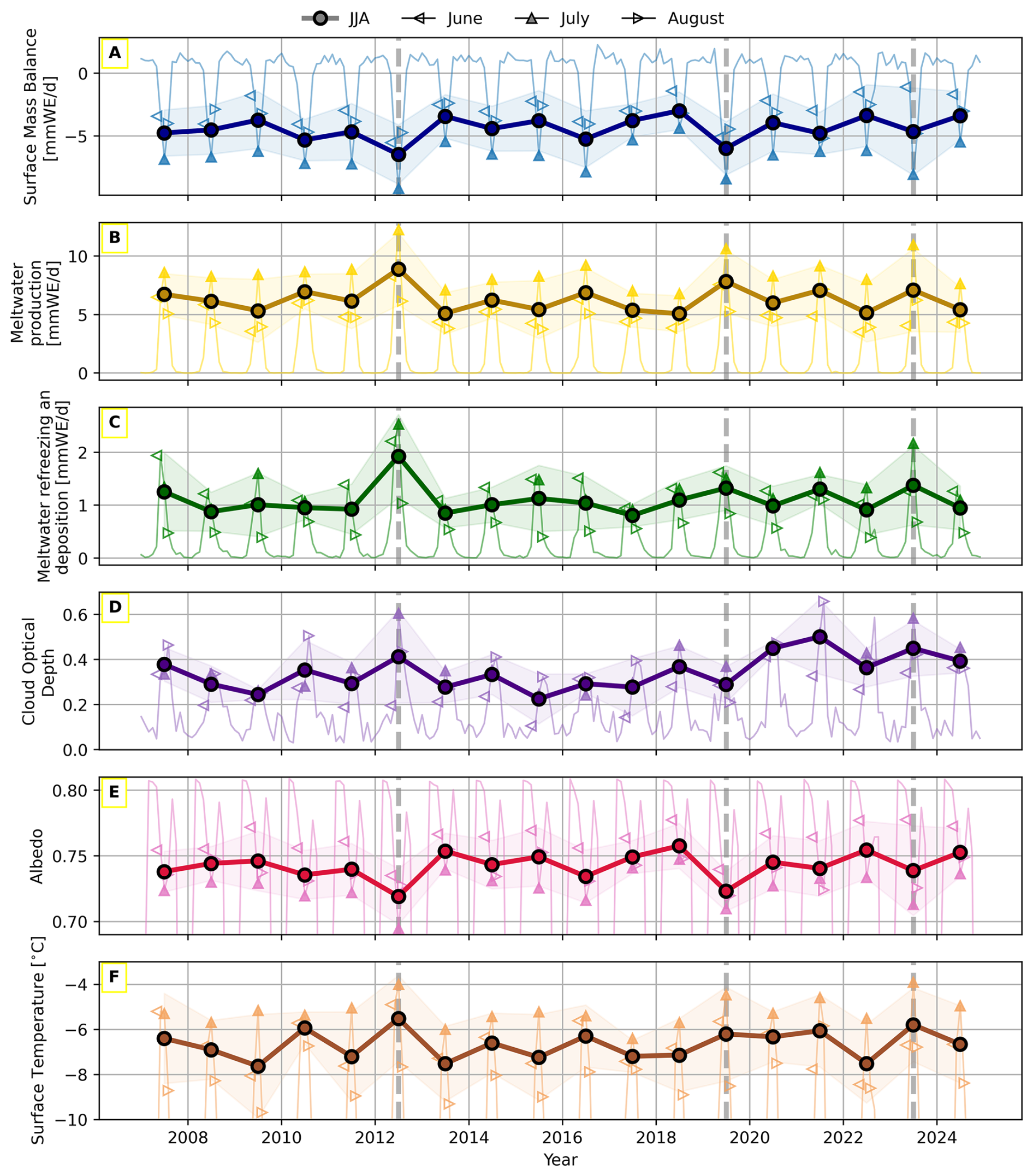
Figure 6 Time series of average (A) surface mass balance, (B) meltwater production, (C) meltwater refreezing and deposition, (D) low cloud cover, (E) albedo, and (F) surface temperature as simulated by the Modèle Atmosphérique Régionale (MAR), respectively. Filled circles connected by thick solid lines show only the June–July–August (JJA) averages, while the thinner line depicts the full monthly dataset. June, July and August means are all individually represented by left, up and right-facing triangels, respectively. All points in the time series represent Greenland-wide spatial averages weighted by latitude for the respective parameter. The semi-transparent sleeves around the main data represents one standard deviation (calculated over the averaging period). Vertical dashed gray lines represent the anomalous summers of interest: 2012, 2019 and 2023. The pearson correlation coefficient reported in the legend is computed between the JJA averages of the parameters shown in each subplot.

Looking at model results from MAR in Fig. 6, we can consider the GrIS as a whole as opposed to just the surface layer and the atmosphere above it. Here again we see that the three summers of interest, highlighted by the gray dashed lines, stand out when viewing the 2007–2024 time series. The SMB was most negative in 2012 and 2019, respectively, however in terms of average meltwater production, the summer of 2019 and 2023 were within 1 mm of Water Equivalent per day (mmWE d⁻¹) of each other, with the 2023 July average (filled upward-facing triangle) surpassing that of 2019 by >0.3 mmWE d⁻¹. The average meltwater refreezing and deposition exceeded 2 mmWE d⁻¹ only in the Julys of 2012 and 2023, respectively (see Fig. 6C). Notably, July average cloud optical depth is highest in 2012, followed closely by 2023 (Fig. 6D). Meanwhile albedo (Fig. 6E) shows the same variation in time as $R_{\mathit{\lambda }}^{\mathrm{TOA}}$ (Fig. 5A), which helps link the model results to our satellite measurements. MAR surface temperature (Fig. 6F) is similar to ERA5 2 m temperature (Fig. 5C), which is expected given that the reanalysis is used to force the regional model.

4 Discussion

4.1 Using top-of-atmosphere reflectance to study periods of extreme melt

This study demonstrates that changes in $R_{\mathit{\lambda }}^{\mathrm{TOA}}$ in the visible/near-infrared offer a good assessment of the state of the GrIS during summers with extreme melt. Through the analysis of this quantity, we identified the anomalous summer of 2023. While the summer 2023 Greenland-wide $R_{\mathit{\lambda }}^{\mathrm{TOA}}$ average is still above that of the summers of 2012 and 2019, primarily due to the the strong negative values concentrated on the southwestern coast in 2012 and 2019, it nevertheless sets itself apart by having negative anomalies all across the GrIS in both the JJA (Fig. 2C) and July (Fig. 3C) average maps. These anomalies are nearly all one standard deviation below the 2007–2024 mean, highlighting the event's anomalous nature.

Rather than developing additional higher-level retrievals, we made use of the assumption-free $R_{\mathit{\lambda }}^{\mathrm{TOA}}$ measurements directly and quantified their statistical relationships with in situ observations, satellite-derived products, reanalysis datasets, and model simulations. Through these analyses, we have found that $R_{\mathit{\lambda }}^{\mathrm{TOA}}$ is primarily driven by surface conditions on top of the glacier, specifically over the high-albedo accumulation zone. Through radiative transfer modeling, Lelli et al. (2023) showed (in Fig. 1 of their study) that clouds over Greenland do not reduce $R_{\mathit{\lambda }}^{\mathrm{TOA}}$, even in the presence of snow below. Thus, given the predominantly forward-scattering nature of both liquid and ice clouds, the negative $R_{\mathit{\lambda }}^{\mathrm{TOA}}$ anomalies seen for the central Greenland region in Fig. 2A are likely caused by the surface. Despite the lack of strong absorption bands for ice and snow in the 576–790 nm range used for the calculation of $R_{\mathit{\lambda }}^{\mathrm{TOA}}$, already at 600 nm the absorption coefficient begins to increase for glacial ice as well as snow (Cooper et al., 2021). Reduced subsurface scattering is another reason why $R_{\mathit{\lambda }}^{\mathrm{TOA}}$ may decrease, which in the context of the GrIS can be attributed to snow melt. Specifically, the increase in grain size due to melt (Colbeck, 1982) and the associated reduction in scattering opportunity increasing the absorption probability for individual photons (Warren, 2019). Clouds contribute to the reduction of $R_{\mathit{\lambda }}^{\mathrm{TOA}}$ by facilitating surface melt over the accumulation zone where the annual longwave cloud radiative forcing is 33 Wm⁻² (Miller et al., 2015). Thus, while clouds do not directly reduce $R_{\mathit{\lambda }}^{\mathrm{TOA}}$ in the 576–790 nm range that we look at, their longwave warming effects, in the presence of warm moist air brought forth by favorable atmospheric circulation, lead to the reduction $R_{\mathit{\lambda }}^{\mathrm{TOA}}$ over the central Greenland region by helping melt the surface. This indirect effect is nicely captured in the July $R_{\mathit{\lambda }}^{\mathrm{TOA}}$ maps (Fig. 2), especially for 2023 (Fig. 2C). Over the ablation zone and exposed land area on the western coast of Greenland, clouds increase the reflectance, and this is what we see when comparing Figs. 2A with 4C, F and I: the positive cloud anomaly, caused by ARs from the south and southwest, causes an increase in $R_{\mathit{\lambda }}^{\mathrm{TOA}}$ over the Baffin Bay, Greenland coast and the lower elevations of the GrIS, while causing a decrease over the high elevation accumulation zone. On the other hand, under cloud-free conditions in the summer of 2019, the western coast experienced more melting along the ablation zone which exposed more dark, bare ice (Tedesco and Fettweis, 2020), which resulted in a $R_{\mathit{\lambda }}^{\mathrm{TOA}}$ decrease for the region (see Fig. 2B). In this way GOME-2 $R_{\mathit{\lambda }}^{\mathrm{TOA}}$ provides additional information that complements passive microwave data products like GIST. Namely, passive microwave observations are typically interpreted as a binary melt/no-melt classification based on thresholding brightness temperatures (e.g. Mote, 2007; Colosio et al., 2021), whereas GOME-2 $R_{\mathit{\lambda }}^{\mathrm{TOA}}$ provides continuous information on surface reflectance and albedo, as well as cloud radiative properties, both of which influence the surface energy balance and are linked to melt variability and preconditioning.

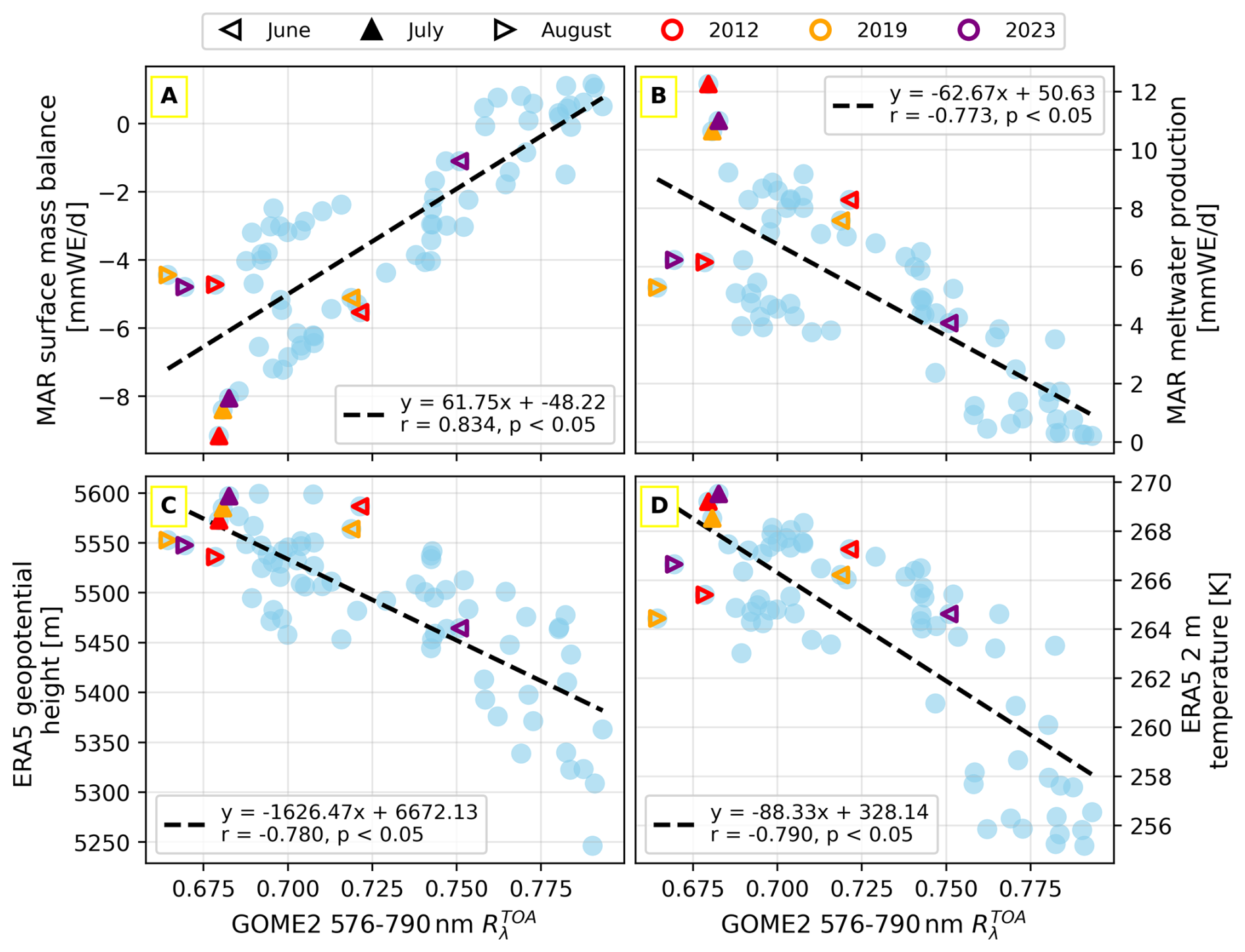
Figure 7 GOME-2 $R_{\mathit{\lambda }}^{\mathrm{TOA}}$ plotted against (A) MAR surface mass balance, (B) MAR meltwater production, (C) ERA5 geopotential height, and (D) ERA5 2 m temperature. Each point is a Greenland-wide average for May, June, July and August within the 2007–2024 time frame. June, July and August means for 2012, 2019 and 2023 are all individually represented by left, up and right-facing triangels, respectively, with colors corresponding to the years of interest.

In Fig. 7, we show the relation between $R_{\mathit{\lambda }}^{\mathrm{TOA}}$ and correlated parameters for individual months based on their evolution in Figs. 5 and 6. Here May is included in addition to JJA since the melt season typically begins already in the first half of May, especially in recent years (Colosio et al., 2021). Months with colored triangles represent the summer months from the years of interest. Interestingly, in August the Greenland-wide $R_{\mathit{\lambda }}^{\mathrm{TOA}}$ average is lower than in July, which is when all y-axis parameters in Fig. 7 are typically at their maximum (minimum in the case of SMB). This behavior arises from the increased atmospheric path length associated with a larger solar zenith angle in August. Such an increase enhances the attenuation and scattering of solar radiation by the atmosphere and consequently reduces the observed radiance, and by extension, the $R_{\mathit{\lambda }}^{\mathrm{TOA}}$. Despite this influence, all correlations r are above 0.7, demonstrating the link between $R_{\mathit{\lambda }}^{\mathrm{TOA}}$, GrIS surface properties, and related parameters.

4.2 State of the Greenland Ice Sheet in Summer 2023 Compared with 2012 and 2019

Figures 2 through 6 underline the exceptional nature of the summers of 2012 and 2019, but also 2023. The 2023 average Greenland-wide July ERA5 2 m temperature at 271 K is the highest on record since 1979, surpassing 2012 when only July is considered, and coming second when averaging over JJA. The spatial distribution of these high temperatures across the GrIS can be observed in Fig. 3F, and to a lesser extent in Fig. 2F, even though the colder month of June is pushing down the JJA averages. Importantly, the warm temperature anomaly was not just at the surface but also above the boundary layer in the free atmosphere. The ERA5 700 hPa Greenland-wide July temperature average also surpassed that of 2012 by >0.3 K, while coming in second over the 2007–2024 time frame when considering JJA (see Figs. D2 and D1 in Appendix D). At 500 hPa, both July and JJA 2023 averages are surpassed by 2012 values. With such high temperatures, the average melt extent was more than 6.0×10⁶ km² in the July of 2023 as observed by SSMIS, with the average meltwater production at 11.0 mmWE d⁻¹ and a total of 441.3 Gt meltwater produced throughout the month according to MAR. This puts the 2023 July melt extent average more than 1.0×10⁶ km² above every other July average since 1979 except that of 2012 at 7.2×10⁶ km². It is second also in terms of the JJA melt extent average with a narrower margin of $\sim \mathrm{2.0}\times {\mathrm{10}}^{\mathrm{5}}$ km², as well as the average and total meltwater produced in the month of July with margins ∼0.2 mmWE d⁻¹ and ∼30 Gt, respectively. In terms of the melt extent average, the summer, and by extension July, of 2019 is unremarkable because meltwater production was mostly restricted to the ablation zone. However, the JJA average and total amounts of meltwater produced are greater than for the summer of 2023, but the opposite is true for the month of July. Moreover, the July and August conditions of 2023 were comparable in severity and impact to the widely studied melt seasons of 2012 and 2019. Were it not for the colder month of June, the 2023 melt season would likely be more prominently represented in the scientific literature. As such, this study draws attention to this overlooked event and provides a detailed analysis of the characteristics and behavior of such extreme melt summers.

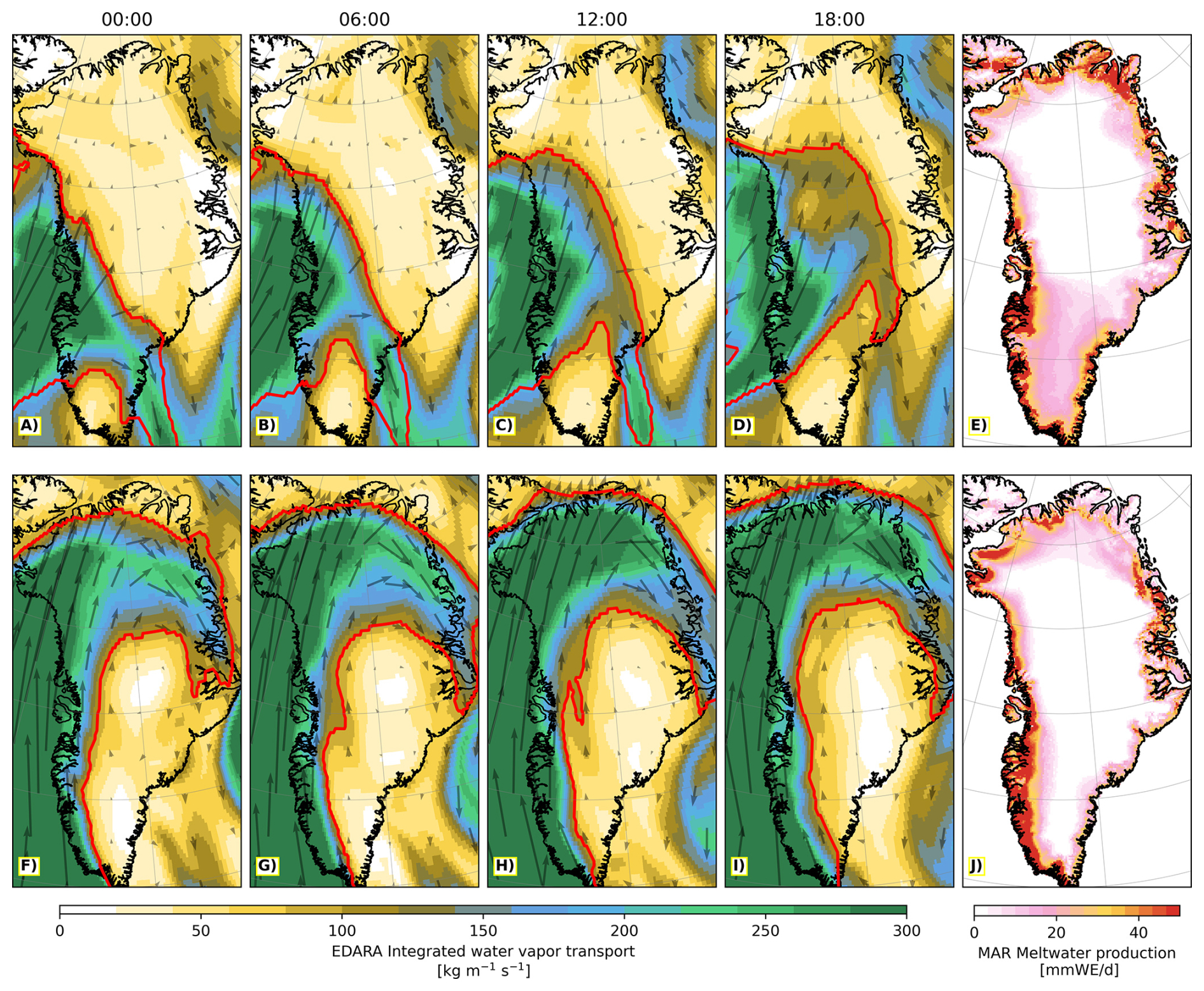
Figure 8 Greenland maps from the ERA5-based Dataset for Atmospheric River Analysis (EDARA) as well as Modèle Atmosphérique Régionale (MAR). Subplots (A)–(D) and (F)–(I) show EDARA integrated water vapor transport (IVT) maps in 6 h increments for the days of 7 July and 22 August of 2023, respectively, while subplots E and J show meltwater production, for those same dates, simulated by MAR. In the EDARA maps, the arrows provide directional information about the IVT, and the red outline shows atmospheric rivers identified by the Tracking Atmospheric Rivers Globally as Elongated Targets v3 algorithm.

In Fig. 1, two major episodes of melt stand out in the summer of 2023, the prolonged one in July and the rather brief one in August. The July episode begins with the first peak around 7 July and continues until 24 July, whereas the August episode peaks on 22 August and lasts a total of around 6 d. For both 7 July and 22 August, Fig 8 shows the EDARA IVT from 00:00 to 18:00 UTC. The influence of the ARs on both these days can be seen wherein the part of the GrIS that exhibits widespread melt according to MAR corresponds well with where the AR is directing the warm moist air from the South. In Fig. 3I, the wind and geopotential height anomalies for July 2023 show a rather pronounced inflow of air from the southwest, forced by an anticyclone centered on the southern tip of Greenland. Thus, the pattern we see in Fig 8A–D, is consistent with the average for the month. In Fig 3G, a similar pattern can be observed for the July of 2012, wherein southerly winds, forced by an anticyclone, bring warm moist air masses onto the GrIS (for AR information during melt peaks, see Fig. B1 in Appendix B). During the melt peak of the summer of 2019 (30–31 July) an easterly AR is identified by the tARget-v3 algorithm (see Fig. B2 in Appendix B), corroborated by the easterly wind anomaly in Fig. 3. The key difference seems to be that while in the summer of 2012, the ARs typically managed to push their moisture onto the ice sheet from the south to the north, the easterly ARs of 2019 were partly inhibited by Greenland's mountainous eastern coast. In addition, Tedesco and Fettweis (2020) report that these easterly air masses were drier in comparison to 2012, which limited the formation of liquid clouds (as seen in the GrIS-wide negative cloud cover anomaly in Fig. 4). In contrast, in the summers 2012 and 2023, the moisture brought by ARs led to a clear increase in cloud cover and TCLW (see Fig. 4), suggesting both the presence and absence of clouds can lead to melt.

From the time series figures (Figs. 5 and 6), we can make further distinctions between these two scenarios when comparing the summer of 2019 to that of 2012 and 2023. All three summers exhibit a low $R_{\mathit{\lambda }}^{\mathrm{TOA}}$ average (Fig 5A) and high GBI (Fig 5B). While average retrieved melt area and surface temperature is less in the summer of 2019 (Figs. 5C, D and 6F), it falls between 2023 and 2012 in average meltwater production and SMB (Fig. 6A and B). The parameters in which we see clear differences are cloud cover and TCLW (Fig. 5E and F), wherein we can see $R_{\mathit{\lambda }}^{\mathrm{TOA}}$ drop alongside cloud cover and TCLW from 2018 to 2019, and vary inversely during 2011–2012 and 2022–2023, respectively. Additionally, the average meltwater that was refrozen and deposited as simulated by MAR (Fig. 6C) was high in the summers of 2012 and 2023, but not in 2019. The primary difference between the extreme melt summers of 2012 and 2023 can be summed up as 2023 having been a 2012-type event over a shorter time-span, wherein it only began in late June. Anomalous melt in June preconditioned the GrIS for additional melt episodes in both the summers of 2012 and 2019, but not in 2023. However, aside from the differences in duration and therefore severity, 2012 and 2023 summer share the positive cloud cover and TCLW anomalies, the near-melting temperatures across the GrIS and as shown later in Fig. 9, high cloud optical depth over the ablation and accumulation zones.

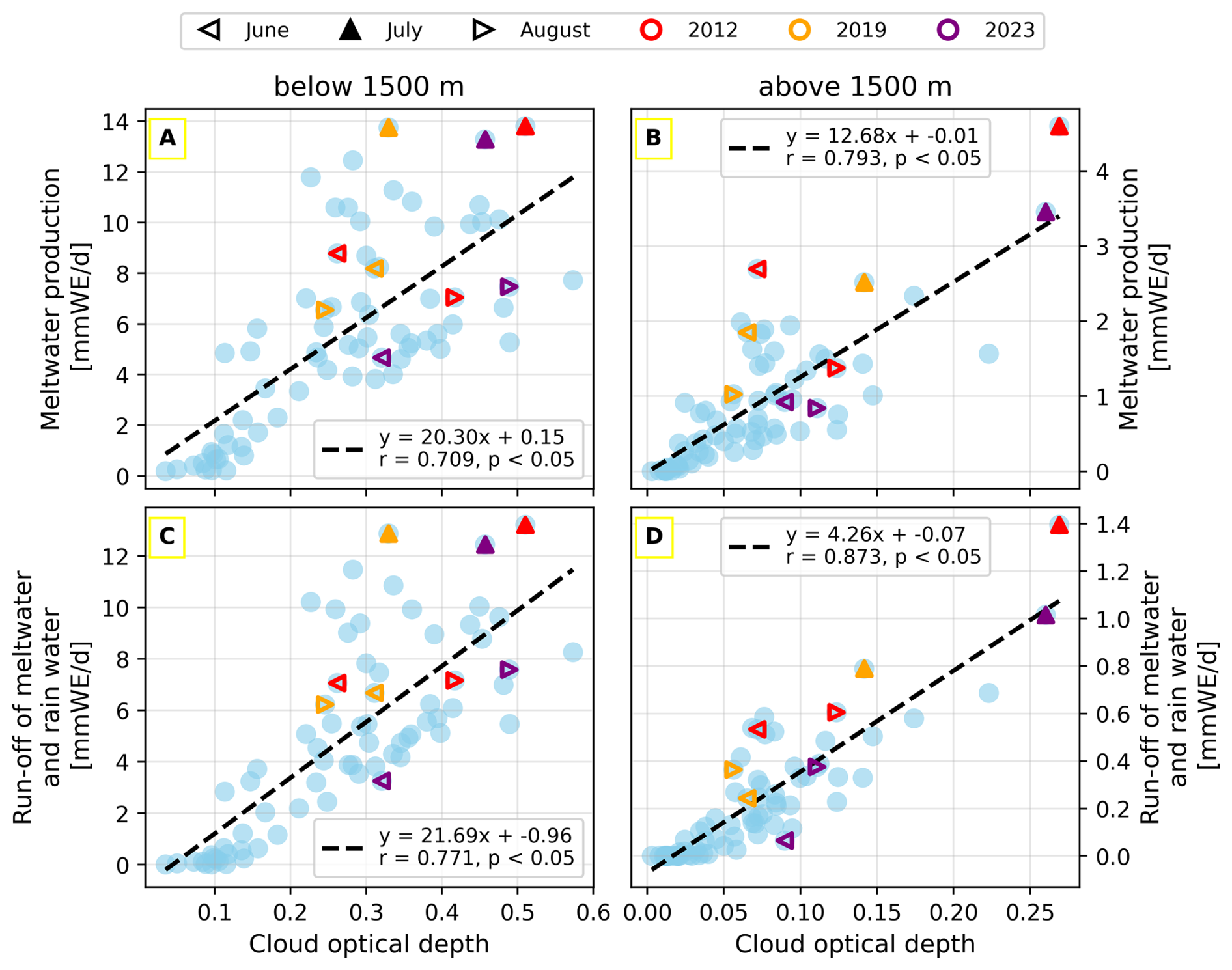
Figure 9 Cloud optical depth plotted against (A–B) meltwater production and (C–D) run-off of meltwater and rain water, such that the left column (A, C) corresponds to averaged values below 1500 m and the right column (B, D) corresponds to averaged values above 1500 m. Each point is a Greenland-wide average for May, June, July and August within the 2007–2024 time frame. June, July and August means for 2012, 2019 and 2023 are all individually represented by left, up and right-facing triangels, respectively, with colors corresponding to the years of interest. All parameters are taken from Modèle Atmosphérique Régionale (MAR) runs forced by ERA5 reanalysis.

4.3 The relationship between clouds and surface melt during extreme melt summers

The role of clouds in contributing to surface melt across the GrIS is not straightforward. Low-level liquid clouds have been shown to play a crucial part in the 2012 summer anomaly by also causing melt at higher elevations (Bennartz et al., 2013), thereby propagating melt across the entire GrIS (Nghiem et al., 2012). Studies like Miller et al. (2015) have since shown that over the accumulation zone, in areas with high surface albedo, liquid clouds are persistent contributors to surface melt through longwave warming effects in all months. Van Tricht et al. (2016) go further to say that clouds enhance meltwater run-off by one-third relative to clear skies across the GrIS, including the ablation zone. Thus through a combination of longwave warming during the day and by suppressing refreezing during the night, which is especially relevant for the ablation zone where bare ice is exposed and vulnerable (Van Tricht et al., 2016), clouds supposedly contribute to melt throughout the GrIS.

On the other hand, studies like Blau et al. (2024) stress that it is the clear-sky downwelling longwave radiation and the surface albedo feedback, paired with atmospheric circulation anomalies, that contribute most to extreme warming events. While studies like Hofer et al. (2017) point out that a decreasing summer cloud cover trend enhanced the melt-albedo feedback, and thereby lead to more melt since the 1990s, especially in the ablation zone.

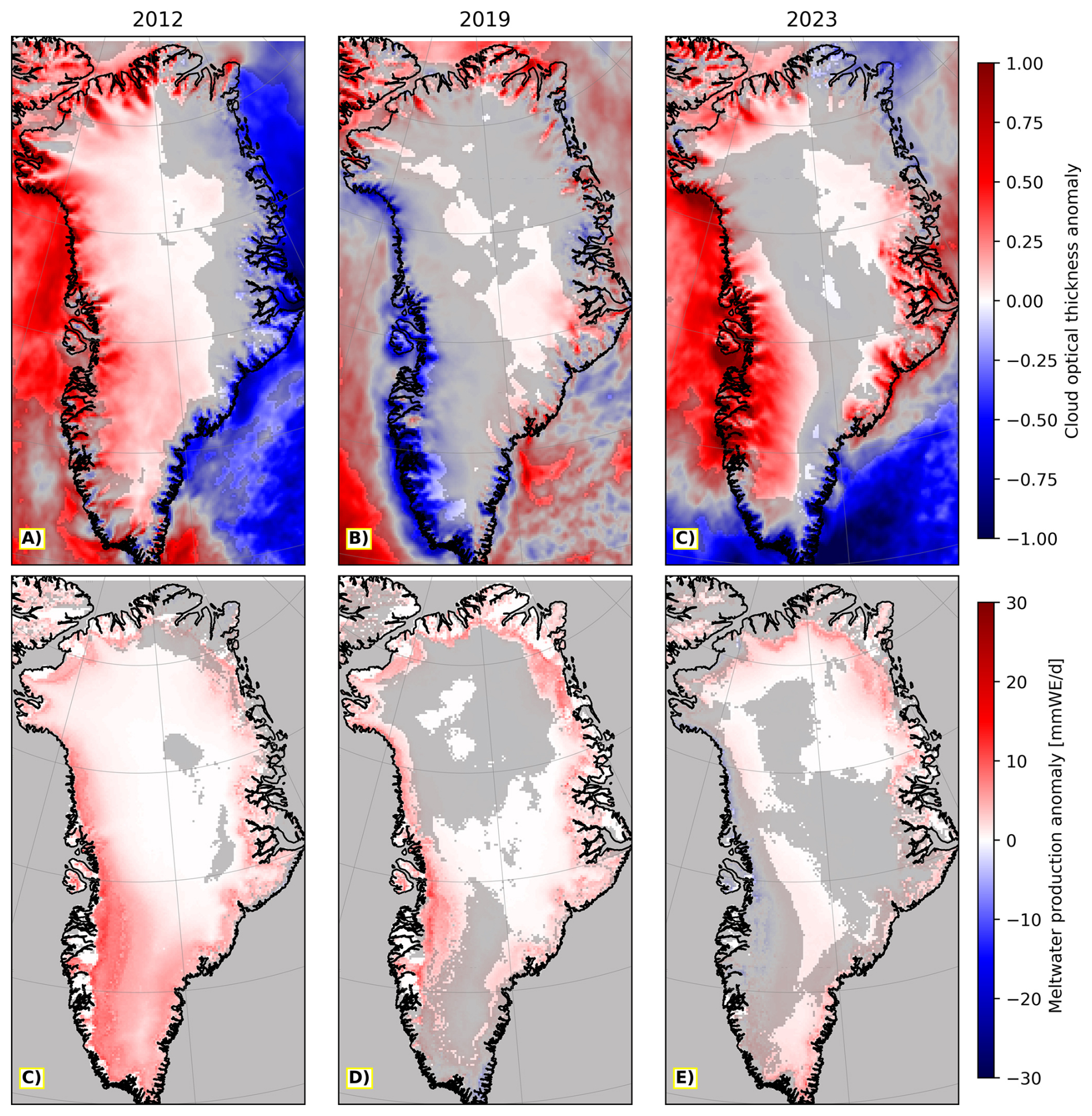
Figure 10 Maps of June–July–August (JJA) (A–C) cloud optical thickness anomaly and (C–E) meltwater production anomaly as simulated by Modèle Atmosphérique Régionale. The left, center and right columns correspond 2012, 2019 and 2023, respectively. All anomalies are calculated for the JJA of each year with respect the 2007–2024 JJA mean. Grid cells without a gray filter are one standard deviation away from the mean.

Figures 9 and 10 help demonstrate the relationship between surface and cloud properties as simulated by MAR v3.14.3. For Fig. 9, we use a height of 1500 m above sea level as a static threshold to investigate how cloud optical thickness varies with meltwater production and run-off in the ablation and accumulation zones. Although MAR also simulates SMB, instead of using the equilibrium line altitude (the elevation at which snow accumulation balances ice melt and SMB equals zero), we use an elevation-based estimate to provide a fixed threshold that is less sensitive to inter-summer variability. Figure 9A and C shows that the months of July from the years 2012, 2019 and 2023 have the highest average melt and run-off, respectively. However, the average July cloud optical depth value noticeably lower in 2019 than in 2012 and 2023, especially over the accumulation zone. Meanwhile, in Fig. 9B and D, we see that July 2019 is overtaken by July 2023 values in both average meltwater production and run-off and is in general closer to the line of best fit. This discrepancy supports the findings of Bennartz et al. (2013) and Miller et al. (2015), wherein over the accumulation zone (above the threshold), liquid clouds contribute to surface melt through longwave warming effects. Whereas below the threshold, clear-sky downwelling longwave radiation also plays an important role, especially over exposed bare ice which is relatively dark.

It is important to mention here that all the data shown in Figs. 9 and 10 is from MAR v3.14.3. Mattingly et al. (2020) reported that MAR v3.9.6 had a negative bias in net shortwave radiation for parts of the accumulation zone, especially during strong AR events. Similarly, v3.9.6 severely underestimated cloud liquid amounts by overestimating cloud ice phase, also during AR conditions. As cloud liquid droplets are the primary drivers in cloud-induced longwave warming over the accumulation zone, this bias will impact the modeled values. While multiple improvements have been implemented with each version update since v3.9, they were primarily aimed at improving surface property representation (Mankoff et al., 2021; Antwerpen et al., 2022) and adapting new radiative schemes (Fettweis et al., 2021; Grailet et al., 2025). Thus, it is highly likely that MAR still underestimates the melt response to AR-initiated liquid cloud melt events like those in the summers of 2012 and 2023. As a result, it is important to also consider satellite and in situ measurements, such as GOME-2 $R_{\mathit{\lambda }}^{\mathrm{TOA}}$ and AWS measurements, rather than relying on regional model output alone.

5 Conclusions and Outlook

In this study we addressed our three primary objectives outlined at the end of the introduction section. We used a synergistic approach combining measurements (GOME-2 $R_{\mathit{\lambda }}^{\mathrm{TOA}}$) with higher-level satellite, reanalysis, and model-derived data products, together with in situ observations from AWS, to perform a comprehensive analysis of extreme melt summers. As discussed in Sect. 4.1 addressing objective 1, $R_{\mathit{\lambda }}^{\mathrm{TOA}}$ proved to be a a reliable direct measurement of the severity of melt across the GrIS during extreme melt summers like 2012, 2019 and 2023.

We assessed the parameters that both precondition and help quantify the severity of the summer anomalies in both time and space, in conjunction with our $R_{\mathit{\lambda }}^{\mathrm{TOA}}$ measurement. Collectively, the Greenland-wide average $R_{\mathit{\lambda }}^{\mathrm{TOA}}$ values from the summers of interest are lower than those observed in any other year since the start of the GOME-2 record in 2007. Consequently, the summer of 2023 was identified as an anomaly comparable to that of 2012 and 2019 such that together, these three summers exhibit higher average ERA 2 m temperatures, SSMIS surface melt area (not including 2019), and MAR meltwater production than all other years since 1979. As discussed in Sect. 4.2 addressing objective 2, were it not for the anomalously cold June and the associated lack of preconditioning preceding the exceptionally warm July and August of 2023, the summer as a whole would likely have challenged the total melt record set in the summer of 2012.

Lastly, the influence of clouds was assessed through a spatiotemporal analysis of cloud cover, composition, and optical depth derived from satellite observations, reanalysis products, and model output. Based on our discussion in Sect. 4.3 addressing objective 3, we propose that both clear-sky and cloudy conditions can lead to melt through distinct pathways triggered by anomalous atmospheric circulation. Furthermore, whether the strongest melt anomaly occurs in the ablation zone, the accumulation zone, or both depends on the processes that drive anomalous warming during the period of interest.

The principal causes behind anomalously warm summers stem from atmospheric circulation patterns. Namely, the presence of blocking anticyclones, which can help steer ARs around their flanks, thereby enhancing moisture transport to Greenland (Pasquier et al., 2019). As warm, moist air carried by ARs is lifted over the Greenland Ice Sheet, it cools and condenses, increasing local liquid cloud cover (Bennartz et al., 2013; Miller et al., 2015). The cloud cover increases net longwave radiation and enhances turbulent heat fluxes, thereby causing cloud-induced melt. On the other hand, as these ARs cross the ice sheet and descend on the leeward side, clear-sky dry Foehn winds also lead to melt by providing direct sensible heat to the surface (Mattingly et al., 2020). In the absence of ARs over the GrIS, atmospheric blocks contribute to the sinking of warm air and in turn, adiabatic warming. This process dries out the atmosphere, reduces surface albedo and cloud cover, and thereby increases the absorbed solar radiation at the surface which leads to surface melt through a different pathway. This is a pathway that has the strongest effect on the low surface albedo ablation zone surrounding the GrIS and is the pathway that led to anomalous melt in 2019 (Tedesco and Fettweis, 2020). The opposite is true in the summer of 2023, positive cloud property anomalies across the GrIS, especially in the peak melt month of July (see Fig. A1), forced anomalous melt in the accumulation zone, and comparatively little along the margins of the ice sheet. As for the summer of 2012, during peak melt periods in July, both the accumulation and ablation zones experienced melt (Nghiem et al., 2012) as seen in Fig. 10C. For the majority of the ice sheet, especially over the accumulation zone, melt was primarily driven by clouds (see Fig. 10), as in 2023. Importantly, this is not a binary system, and cloud-induced melting likely did occur on the eastern coast of Greenland in July 2019 (See Fig. A1), whereas direct insolation contributed to melt on the Southern tip of Greenland in 2023 (See Fig. 10E), where an anticyclone was present for a significant portion of July (see Fig. 3I). Ultimately, the Arctic climate is changing at a faster rate due to AA, and poleward ARs are projected to increase in frequency, duration and magnitude (Ma et al., 2024). Because of AA-driven atmospheric warming and the resulting reduction in sea ice cover, the Greenland blocking which facilitates these ARs is expected to increase as well (Liu et al., 2016; Sellevold et al., 2022). Furthermore, reduced spring snow cover over northern land masses and the associated terrestrial heating also contribute to the projected increase in Greenland blocking (Preece et al., 2023). Consequently, understanding the dominant processes in future summers, as both atmospheric blocks and the ARs they steer become more frequent, is critical for predicting the future of the GrIS.

A natural extension of this work could be the development of a surface property retrieval exploiting the red end of the visible spectrum and a greater portion of the near-infrared than what is available from GOME-2, where the absorption coefficient for snow and ice is highest (Cooper et al., 2021). In addition, daily data would be superior to monthly averages when comparing against MAR and ERA5. However, a daily visible and near-infrared retrieval would require accurate cloud masking over bright surfaces such as Greenland, which is challenging (Istomina et al., 2020). Additionally, secondary effects, such cloud longwave warming processes observed in the monthly dataset, would be difficult to capture. Such a retrieval would need to clearly demonstrate the advantage it has over passive microwave binary melt/no-melt classification (Mote, 2007) in providing continuous reflectance information, which better captures surface processes such as bare-ice exposure, ice darkening, and snow metamorphosis, despite lacking all-weather, day-and-night observational capabilities. Although the development of such a retrieval was beyond the scope of this study, where the monthly $R_{\mathit{\lambda }}^{\mathrm{TOA}}$ dataset effectively captured Greenland-wide extreme melt summers, it could prove valuable for a more detailed analysis of peak melt periods at the glacier scale.

The methods used in this study would also be applicable to the Antarctic ice sheet. While similar synergistic studies combining satellite, reanalysis, and model data have examined anomalous conditions over parts of the Antarctic Ice Sheet (e.g Gayathri and Laluraj, 2024; Gilbert et al., 2025), visible and near-infrared $R_{\mathit{\lambda }}^{\mathrm{TOA}}$ could provide additional insight into exceptional melt periods. Given the rapid decline in sea ice and the resulting increase in ocean-to-atmosphere heat exchange that influences atmospheric circulation (Josey et al., 2024), this type of research could greatly improve our understanding of the anomalous melt episodes that are likely to occur.

Given climate model uncertainty when it comes to clouds over Greenland (Lacour et al., 2018; Mattingly et al., 2020), observation-based studies such as this one are critical in fine-tuning the influence of clouds over the GrIS during anomalously warm summers. Despite the findings by Liu et al. (2016), Sellevold et al. (2022) and Preece et al. (2023), both Coupled Model Intercomparison Project 5 and 6 reveal decreasing trend of the GBI until 2100 (Hanna et al., 2018; Delhasse et al., 2021). As global models struggle to capture the observed rise in Greenland blocking, there is a high risk that the projected melt of the GrIS does not account for the extreme melt summers that are associated with these atmospheric patterns. As such, differentiating between the unique pathways that lead to record amounts of melt over the GrIS during anticyclonic conditions will help us to better model and predict such anomalies in the future.

Appendix A: Cloud property anomalies for the month of July

In the appendices we include figures that are complementary to our main results. Most of these offer either additional information that supports the main findings or as in the case of Appendix B, additional data on the anomalous summers of 2012 and 2019 for the sake of comparison with Fig. 8.

Here Fig. A1 is shown since both JJA and July are individually featured in Figs. 2 and 3, respectively. However, unlike Figs. 2 and 3, Fig. A1 exhibits a similar anomaly spatial distribution seen in Fig 4 suggesting that the July average strongly influenced the JJA average. As a result, we show it here in the appendix so as not to overcrowd the Results section.

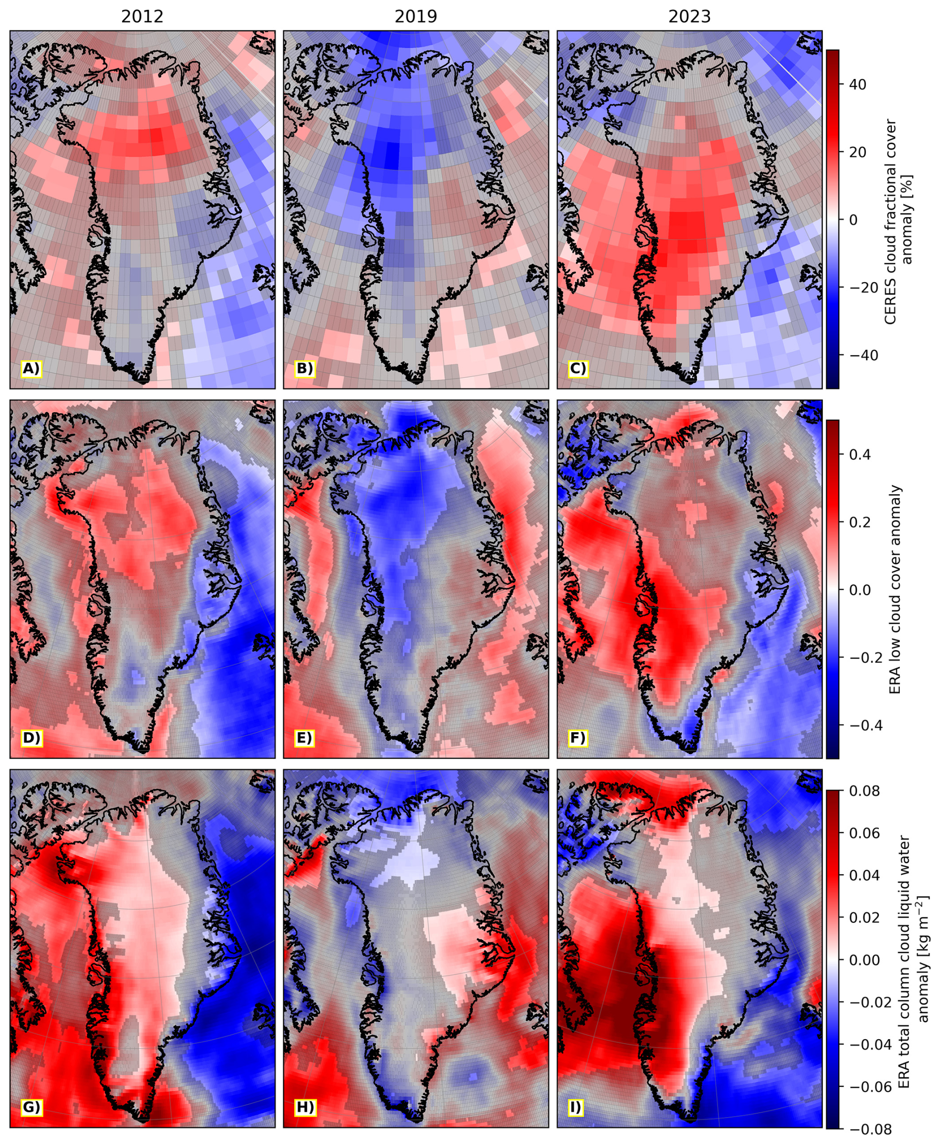
Figure A1 July (A–C) CERES EBAF-TOA cloud cover anomaly, (D–F) ERA5 low cloud cover anomaly or clouds on model levels at ca. 800 hPa, (G–I) ERA5 total column cloud liquid water anomaly. The left, center and right columns correspond to 2012, 2019 and 2023, respectively. All anomalies are calculated for the July of each year with respect the 2007–2024 July mean. Grid cells without a gray filter are one standard deviation away from the mean.

Appendix B: Daily atmospheric river and melt production maps for 2012 and 2019

Figures B1 and B2 are the 2012 and 2019 analogs of Fig. 8, respectively. For Fig. B1, 11 and 28 July of 2012 were selected, corresponding to the two largest peaks in SSMIS melt extent and MAR meltwater production (see Fig. 1). Similarly, 30 and 31 July 2019 are shown in Fig. B2 to illustrate the IVT and atmospheric river conditions associated with the 2019 melt peak.

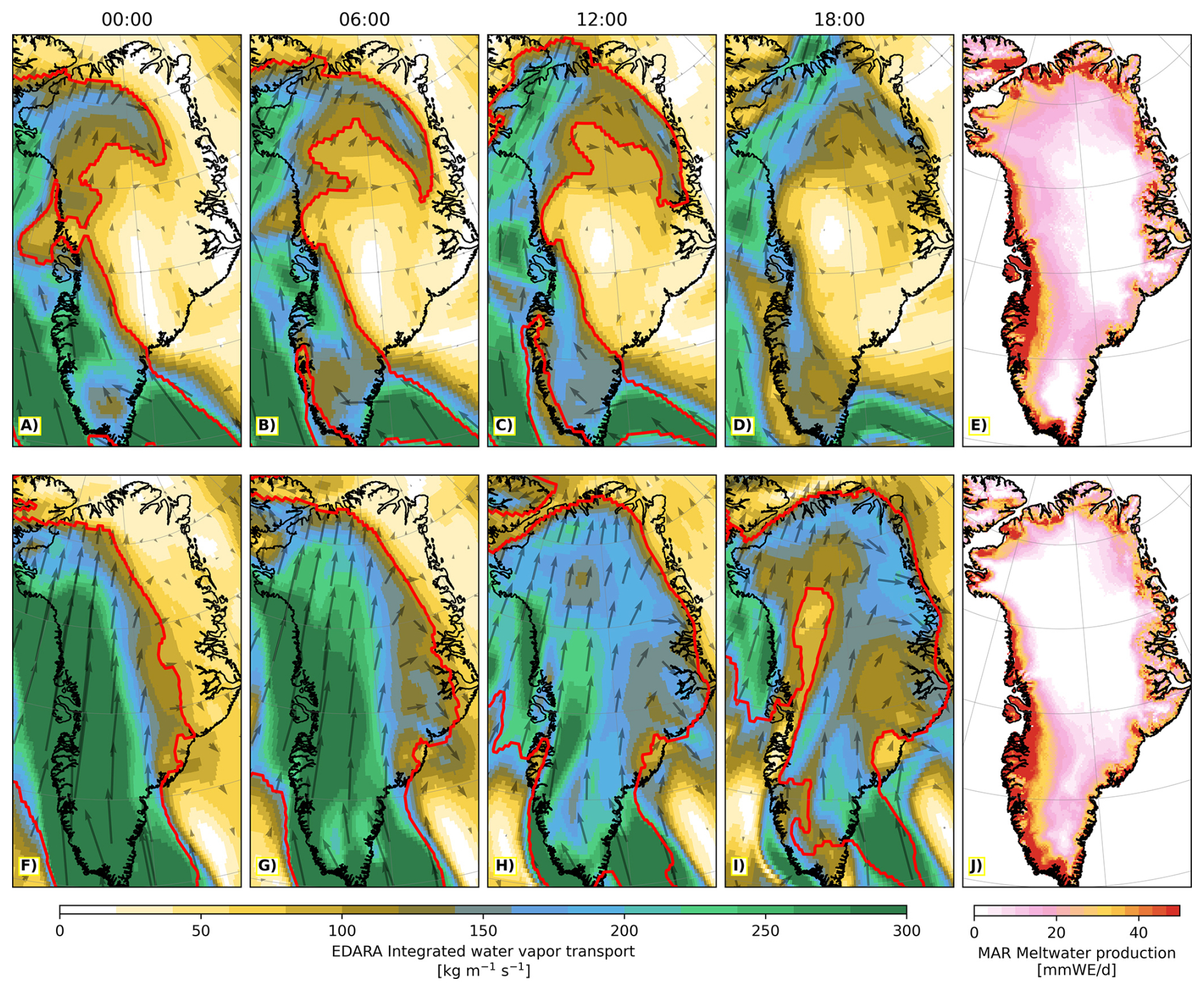
Figure B1 Greenland maps from the ERA5-based Dataset for Atmospheric River Analysis (EDARA) as well as Modèle Atmosphérique Régionale (MAR). Subplots (A)–(D) and (F)–(I) show EDARA integrated water vapor transport (IVT) maps in 6 h increments for the days of 11 and 28 July of 2012, respectively, while subplots (E) and (J) show meltwater production, for those same dates, simulated by MAR. In the EDARA maps, the arrows provide directional information about the IVT, and the red outline shows atmospheric rivers identified by the Tracking Atmospheric Rivers Globally as Elongated Targets v3 algorithm.

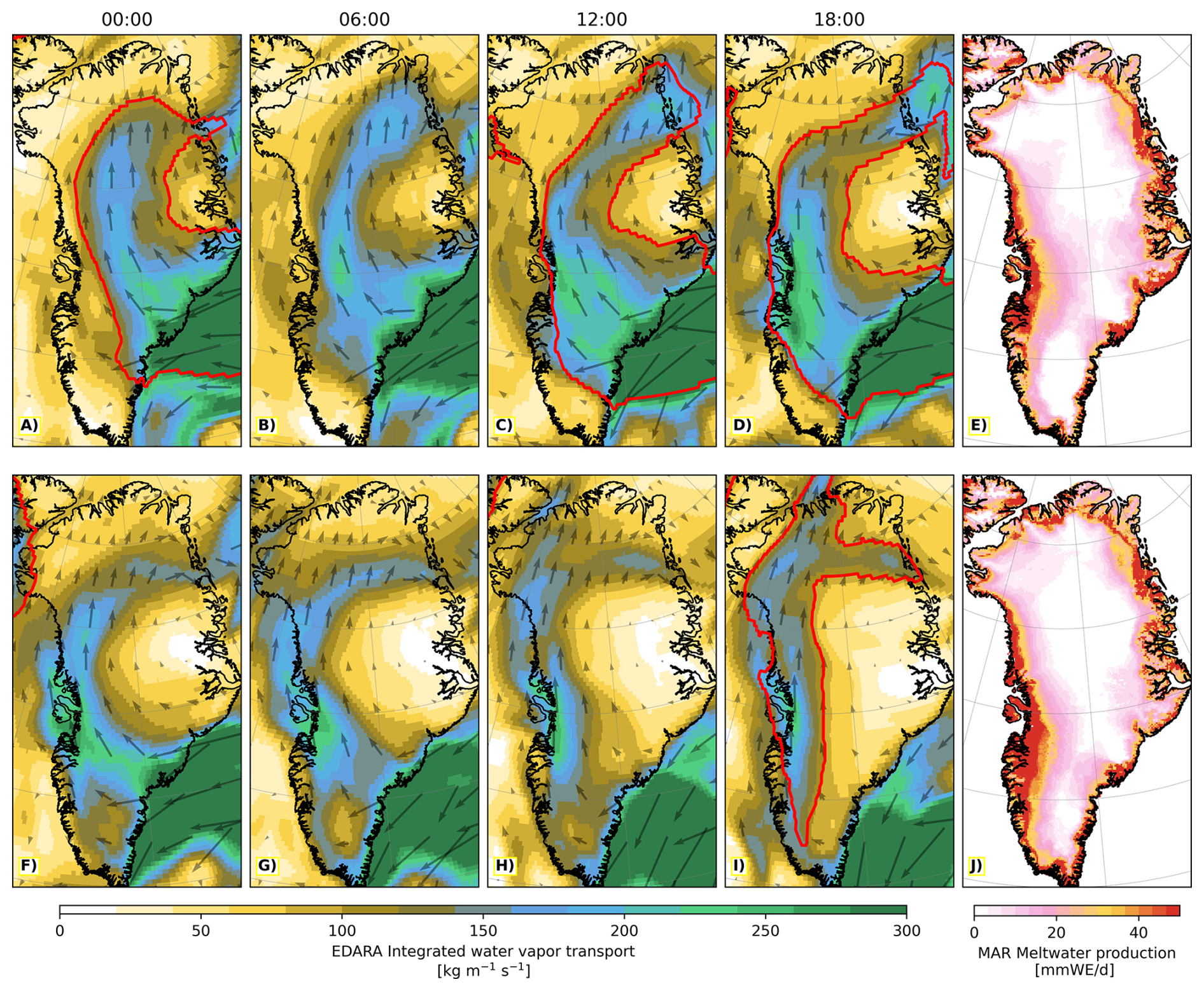
Figure B2 Greenland maps from the ERA5-based Dataset for Atmospheric River Analysis (EDARA) as well as Modèle Atmosphérique Régionale (MAR). Subplots (A)–(D) and (F)–(I) show EDARA integrated water vapor transport (IVT) maps in 6 h increments for the days of 30 and 31 July of 2019, respectively, while subplots (E) and (J) show meltwater production, for those same dates, simulated by MAR. In the EDARA maps, the arrows provide directional information about the IVT, and the red outline shows atmospheric rivers identified by the Tracking Atmospheric Rivers Globally as Elongated Targets v3 algorithm.

Appendix C: Monthly average maps for June and August from the years of interest

In addition to the month of July that takes the focus in our study, the months of June and August are featured here to assess the individual monthly averages that make up Figs. 2 and 4.

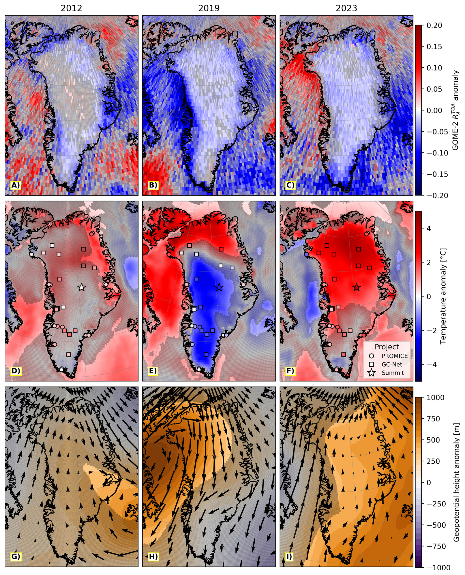
Figure C1 August (A–C) GOME-2 reflectance at the top of the atmosphere ($R_{\mathit{\lambda }}^{\mathrm{TOA}}$) anomaly, (D–F) ERA5 2 m temperature anomaly along with PROMICE/GC-Net automatic weather station temperature anomaly at 2.7 m and Camp Summit anomaly at 2 m, and (G–I) ERA5 geopotential height anomaly at 500 hPa, where arrows represent wind anomaly at 500 hPa. The left, center and right columns correspond 2012, 2019 and 2023, respectively. All anomalies are calculated for the August of each year with respect the 2007–2024 August mean (individual automatic weather station mean values may cover a shorter timeframe based on the operational lifetime of each station). Grid cells without a gray filter are one standard deviation away from the mean.

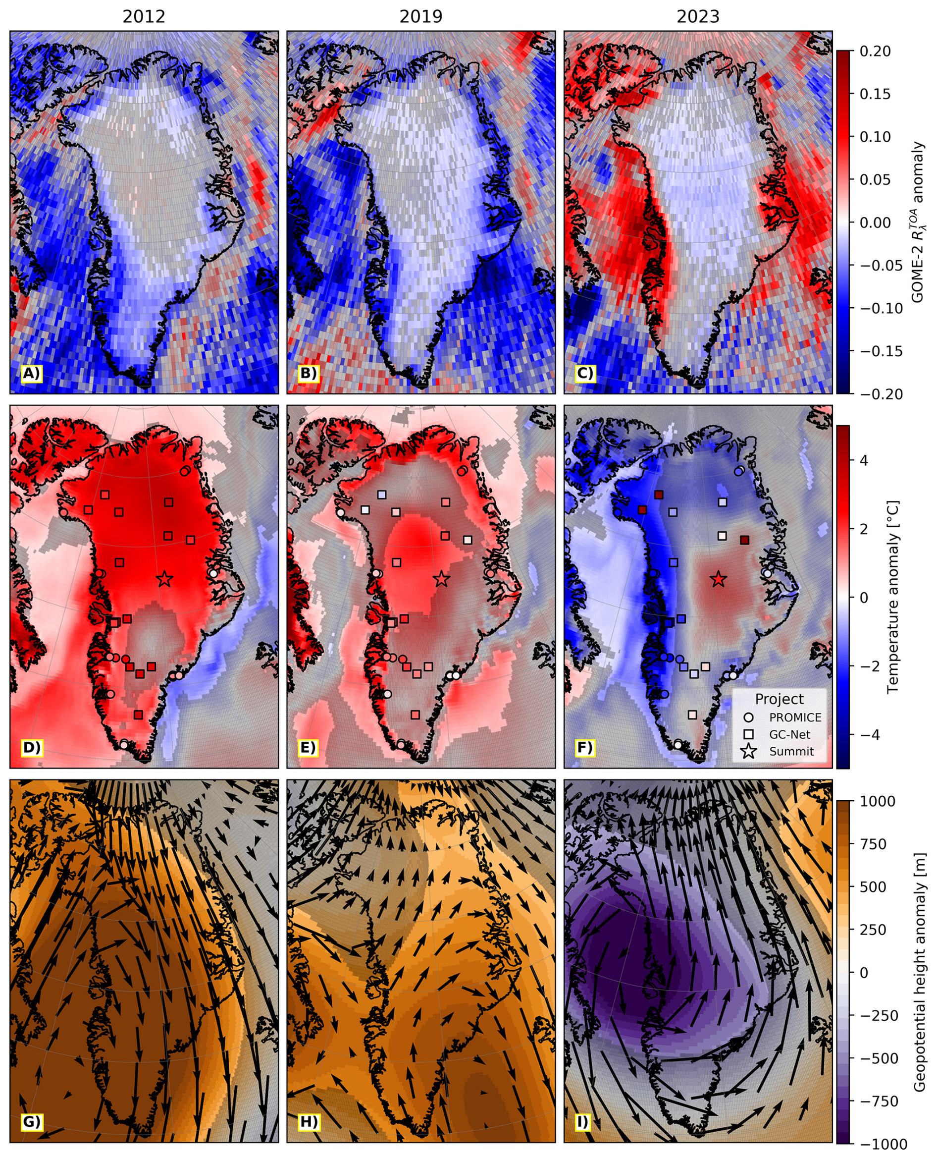
Figure C2 June (A–C) GOME-2 reflectance at the top of the atmosphere ($R_{\mathit{\lambda }}^{\mathrm{TOA}}$) anomaly, (D–F) ERA5 2 m temperature anomaly along with PROMICE/GC-Net automatic weather station temperature anomaly at 2.7 m and Camp Summit anomaly at 2 m, and (G–I) ERA5 geopotential height anomaly at 500 hPa, where arrows represent wind anomaly at 500 hPa. The left, center and right columns correspond 2012, 2019 and 2023, respectively. All anomalies are calculated for the June of each year with respect the 2007–2024 June mean (individual automatic weather station mean values may cover a shorter timeframe based on the operational lifetime of each station). Grid cells without a gray filter are one standard deviation away from the mean.

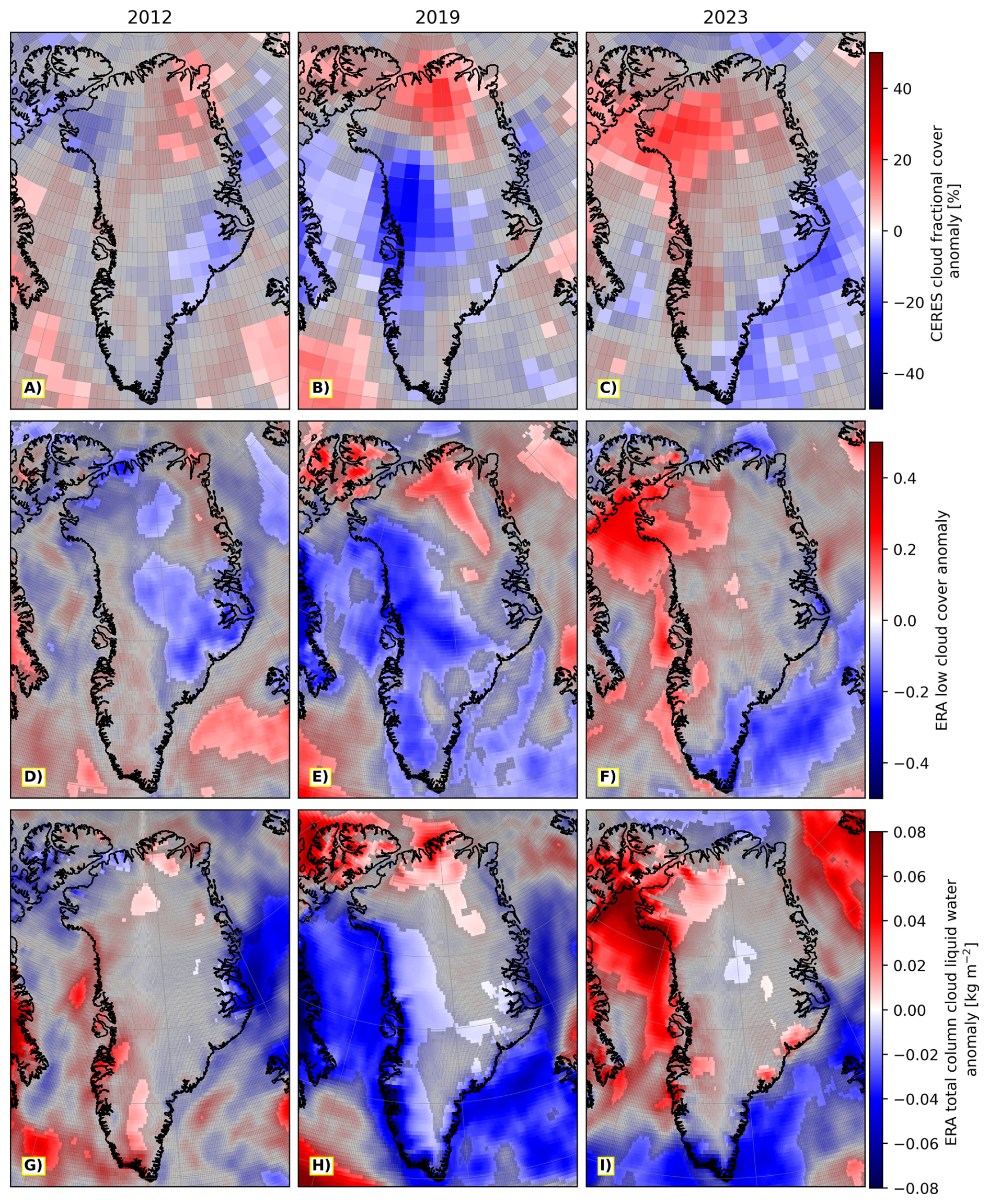
Figure C3 August (A–C) CERES EBAF-TOA cloud cover anomaly, (D–F) ERA5 low cloud cover anomaly or clouds on model levels at ca. 800 hPa, (G–I) ERA5 total column cloud liquid water anomaly. The left, center and right columns correspond 2012, 2019 and 2023, respectively. All anomalies are calculated for the August of each year with respect the 2007–2024 August mean. Grid cells without a gray filter are one standard deviation away from the mean.

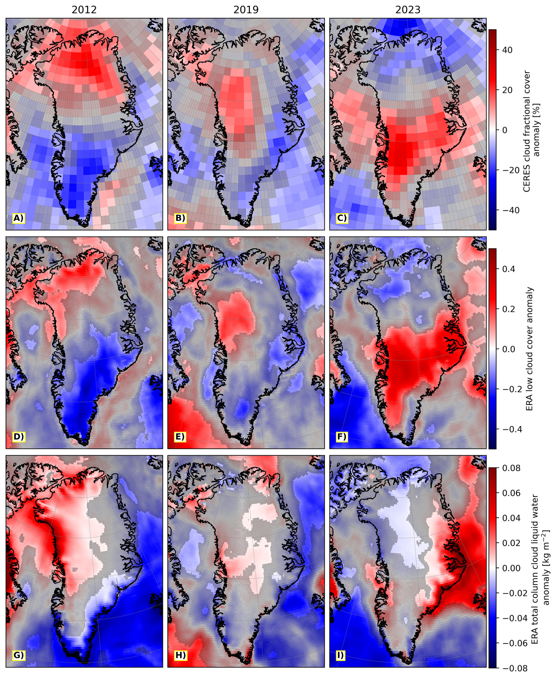
Figure C4 June (A–C) CERES EBAF-TOA cloud cover anomaly, (D–F) ERA5 low cloud cover anomaly or clouds on model levels at ca. 800 hPa, (G–I) ERA5 total column cloud liquid water anomaly. The left, center and right columns correspond 2012, 2019 and 2023, respectively. All anomalies are calculated for the June of each year with respect the 2007–2024 June mean. Grid cells without a gray filter are one standard deviation away from the mean.

Appendix D: JJA and July maps of temperature at 500 and 700 hPa

Since 2 m and skin temperatures are strongly coupled to GrIS surface melt and influenced by melt-related feedbacks, we also include ERA5 temperature anomalies at 500 and 700 hPa. At 500 hPa, the anomalies lie well above the boundary layer and are largely unaffected by surface processes, making them useful for assessing large-scale atmospheric forcing. Meanwhile, the 700 hPa level captures the thermal signature of warm, moist air intrusions, including those associated with ARs, while being less directly affected by surface processes than near-surface temperatures.

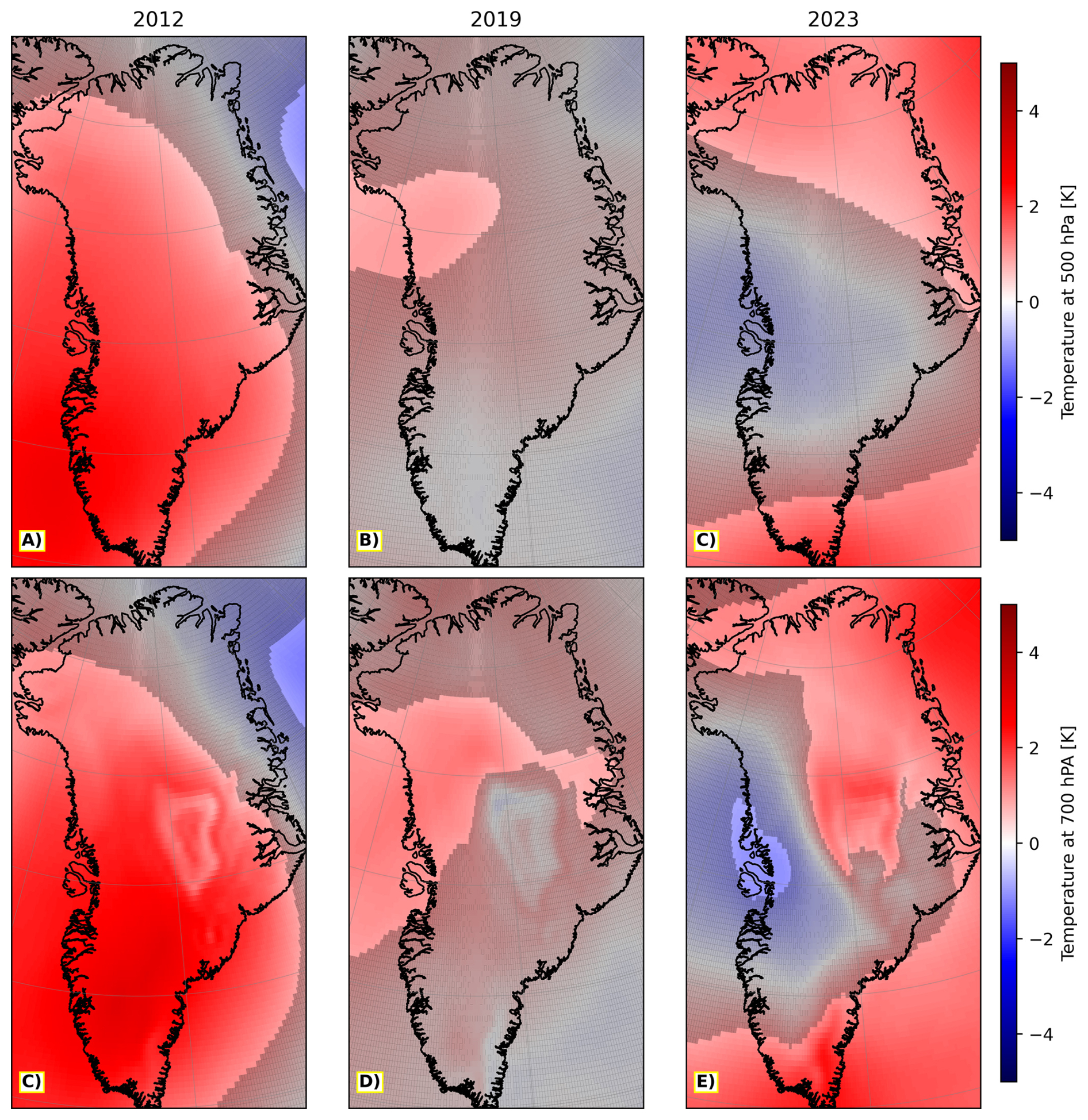
Figure D1 Maps of June–July–August (JJA) ERA5 temperature anomaly at (A–C) 500 hPa and (C–E) 700 hPa. The left, center and right columns correspond 2012, 2019 and 2023, respectively. All anomalies are calculated for the JJA of each year with respect the 2007–2024 JJA mean. Grid cells without a gray filter are one standard deviation away from the mean.

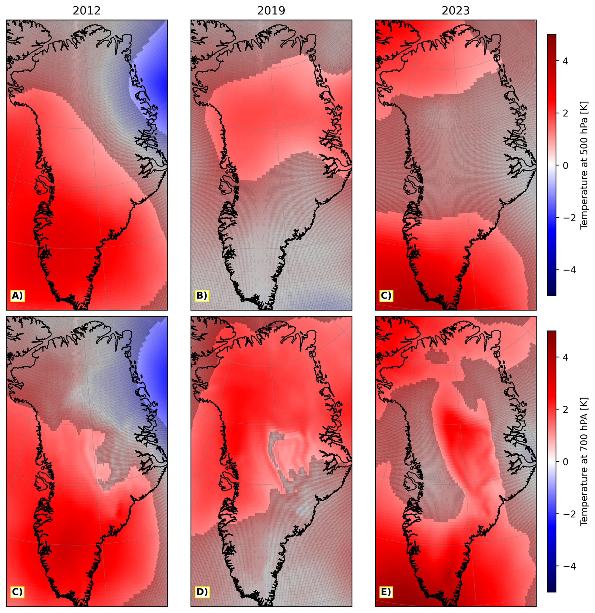
Figure D2 Maps of July ERA5 temperature anomaly at (A–C) 500 hPa and (C–E) 700 hPa. The left, center and right columns correspond 2012, 2019 and 2023, respectively. All anomalies are calculated for the July of each year with respect the 2007–2024 July mean. Grid cells without a gray filter are one standard deviation away from the mean.