Snow depth distributions on sea ice of different ages and thicknesses from regional field campaigns

Accurately representing the snow depth (SND) distribution on sea ice is essential for sea ice thickness (SIT) retrievals, ecological studies, and climate modelling. Using co-located SND and SIT measurements from multiple polar in-situ sea ice campaigns, this study examines sub-kilometre-scale SND variability and identifies the most suitable probability density function (PDF) to represent SND distributions across different ice ages and thicknesses. First, we examine the statistical properties of SND and their dependence on SIT, finding a linear increase in SND with SIT for first-year ice. The coefficient of variation (CV = standard deviation/mean SND) remains constant at 0.50 across all SIT regimes, allowing direct estimation of variability from mean SND. In particular, lower-than-expected SND variability was observed at flooded sites, where snow loading depresses the ice and allows seawater to infiltrate the snow, resulting in a reduced CV. Moreover, the results reveal differences in SND distributions across ice ages and SIT during winter and summer. Specifically, snow over younger ice has a shorter residence time and is best represented by a log-normal distribution, whereas progressive wind-driven redistribution shifts the SND towards a skew distribution. Accordingly, snow over older ice, which typically has a longer residence time, is better represented by a skew distribution. Notably, although the log-normal distribution performs best under specific conditions (e.g. new or melt-season snow), its performance can deteriorate substantially over older and thicker ice, whereas the skew distribution provides a robust representation across heterogeneous ice types. SND correlation lengths derived from semi-variograms show a positive relation with SIT and are enhanced by drifting snow events. These results underscore the importance of ice-condition-dependent parameterizations for representing sub-kilometre SND distribution and improve sub-grid-scale representations of SND variability in remote-sensing retrievals and climate models.

1 Introduction

Over sea ice, snow depth (SND) distributions are controlled by the presence of snow bedforms (e.g. dunes, ripples, or sastrugi) (Filhol and Sturm, 2015), as well as by wind redistribution, seasonal melting, the underlying ice surface (Massom et al., 2001; Herzfeld et al., 2006), and ice age (Warren et al., 1999; Iacozza and Barber, 1999; Trujillo et al., 2016; Shalina and Sandven, 2018; Kochanski et al., 2018; Wagner et al., 2022). A detailed understanding of SND distributions is essential for applying coarse-grid-scale SND products in biological studies, such as determining ideal habitats for ringed seals (Kelly et al., 2010; Chambellant et al., 2012; Iacozza and Ferguson, 2014) and light penetration beneath sea ice (Perovich, 1996; Nicolaus et al., 2012; Arndt et al., 2017). Moreover, an improved understanding of sub-kilometre SND distributions is essential for matching coarse-resolution snow models (tens of kilometres) with the fine spatial resolution of freeboard measurements (hundreds of metres) used to derive sea ice thickness (SIT). To address this, SND redistribution approaches based on sigmoidal functions (Kwok and Cunningham, 2008) or piecewise functions (Kurtz et al., 2009; Petty et al., 2020) have been employed. Glissenaar et al. (2021) demonstrated that small-scale snow variability exerts a significant influence on SIT estimates derived from laser freeboards. Furthermore, SND is a key parameter influencing both the thermodynamic and dynamic processes of sea ice. The spatial variation of SND is essential for understanding snow surface morphology and controls the onset of melt pond formation on level first-year ice (FYI) (Petrich et al., 2012).

Given the high spatial variability of snow cover, even over scales of just a few metres, it is impractical to define modelling units small enough to assume a uniform snow distribution within each unit. A common approach to address this challenge is to use larger modelling units (e.g.  >1 km) while representing sub-kilometre variability through statistical distributions. Due to various meteorological and geophysical processes, snow cover is naturally uneven. Consequently, the assumption of a uniform distribution (Veyssière et al., 2022) cannot accurately represent the SND distribution within a sub-grid cell. To address this, a skew normal distribution (hereafter denoted as skew distribution) based on mean SND (Mallett et al., 2022) has been used in model simulations for under-ice light estimations (Stroeve et al., 2024; Heorton et al., 2025).

Numerous studies have examined SND statistics on terrestrial snow using normal (Marchand and Killingtveit, 2005), log-normal (Donald et al., 1995; Kuchment and Gelfan, 1996; Marchand and Killingtveit, 2004), and gamma distributions (Kolberg and Gottschalk, 2010; Skaugen, 2007; Skaugen and Randen, 2013; Skaugen and Melvold, 2019). For snow on sea ice, Iacozza and Barber (2010) investigated SND on smooth landfast sea ice and reported that probability density functions (PDFs) evolved from a unimodal to a multimodal form with longer tails, indicating the development of deep snow accumulation. These PDFs effectively capture variability in SND and reflect changes under meteorological events such as snowfall and drifting snow (Iacozza and Barber, 2010). Abraham et al. (2015) analysed the effects of sub-grid-scale SND on the transmission of light and heat through sea ice, and implemented Rayleigh-distributed SND to improve the simulation of light fields in sea ice. Mallett et al. (2022) analysed SND measurements taken in straight lines every 10 m along 500–1000 m transects across Arctic sea ice and found that skew distribution provided the best statistical fit to snow depth anomalies over multi-year ice (MYI), with an average coefficient of variation around 0.42. The coefficient of variation (CV) was also calculated for an additional 24 FYI sites by Clemens-Sewall et al. (2024) with a similar mean CV value of 0.42.

Previous studies have revealed that SND distributions depend on ice types. Iacozza and Barber (1999) employed geostatistical analysis using variograms, revealing that SND variability is associated with sea ice age. In particular, FYI showed periodic snow patterns best modelled by Gaussian and wave variograms, while MYI and rubble ice exhibited increasingly irregular distributions, modelled by spherical–Gaussian and single Gaussian variograms, respectively (Iacozza and Barber, 1999). Liston et al. (2020) revealed a linear relationship between parcel age and SND, suggesting that an accurate representation of the evolution of SND on sea ice requires a detailed parcel age on weekly timescales. Itkin et al. (2023) thoroughly investigated the seasonal and ice-type dependence of the SND distribution, showing that the largest snow volumes accumulated by April and that snow on the level ice exhibited a pronounced spatial heterogeneity characterised by snow dunes.

Wind plays an essential role in shaping SND variability and redistribution (Moon et al., 2019). Iacozza and Barber (1999) demonstrated that the geometric anisotropy in the snow distribution was consistently aligned with the prevailing wind directions, highlighting the wind as a dominant control on snow redistribution. Wind influences the spatial distribution of SND across different ice types. For level ice, wind-blown snow tends to accumulate preferentially on younger ice (Clemens-Sewall et al., 2022), where it can form a 2.5–8 cm snow layer by redistributing from adjacent older ice. In addition, snow tends to be transported off level ice and deposited on ridges (Hames et al., 2022) and deformed ice (Merkouriadi et al., 2025) due to wind-driven redistribution. Despite the wind-driven redistribution of SND, Trujillo et al. (2016) examined the impact of a typical storm on SND at high spatial resolution (1–10 cm) over a 100×100 m area, revealing substantial local changes in SND while the overall statistical distribution of surface elevation remained stable.

The aforementioned studies demonstrated that ice ages and wind redistribution are key factors affecting SND distributions on sea ice. Mallett et al. (2022) applied a skew model to SND data from Soviet North Pole (NP) stations, demonstrating superior performance on MYI compared to younger ice. However, since no SIT data are available from these stations, they were unable to investigate the key relationship between SND distribution and SIT. Using co-located SND and SIT data, this study extends prior work by considering a wider range of ice types and by incorporating SIT and meteorological events through time-series analyses. The goal is to improve understanding of the spatial statistical characteristics of SND on sea ice and to determine the most suitable statistical distributions for sub-kilometre-scale SND across varying ice ages and thicknesses.

This study characterises SND variability using data from multiple field campaigns carried out in the Arctic and Antarctic, which are introduced in Sect. 2. Section 3 introduces the statistical distributions and variograms used to characterise SND. Section 4 presents SND statistics, identifies suitable PDFs for different ice conditions, and quantifies spatial variability via correlation lengths, revealing substantial ice-type-dependent differences in sub-kilometre-scale SND variability. The main findings are discussed in Sect. 5 and summarized in Sect. 6. Note that in this article, the ice age refers specifically to FYI, second-year ice (SYI), and MYI, and the ice type denotes broader categories of ice including age and surface condition, such as smooth FYI, deformed MYI, and flooded ice.

2 Data

2.1 Selection of in-situ field campaigns

Two criteria were applied in selecting the datasets. First, since this study aims to investigate the influence of ice age and SIT on SND distributions, it requires coincident in-situ measurements of SND and SIT from diverse ice types. We therefore selected field campaigns spanning a range of ice ages, surface roughness conditions, flooding states, and seasons, while maintaining a balance among sampling sites. Campaigns with well-established contextual knowledge of meteorological events and local ice conditions were prioritized to support the interpretation of the observations. Second, this study aims to analyse the temporal evolution of the SND distribution, which requires time-series observations of snow and ice properties at approximately weekly intervals. Characterizing snow and ice on this timescale is essential to capture snow accumulation and redistribution processes associated with ice growth and meteorological events (Liston et al., 2020).

Table 1 Summary of sea ice thickness (SIT) and snow depth (SND) across all sites. Within each site, co-located SIT and SND measurements were collected over several transects. The number of transects at each site is given in the last column. The mean, median, and standard deviation (SD) of SIT and SND are calculated over all the transects for each site. Ice ages include first-year ice (FYI), second-year ice (SYI), and multi-year ice (MYI), with (F) denoting sites identified as susceptible to flooding.

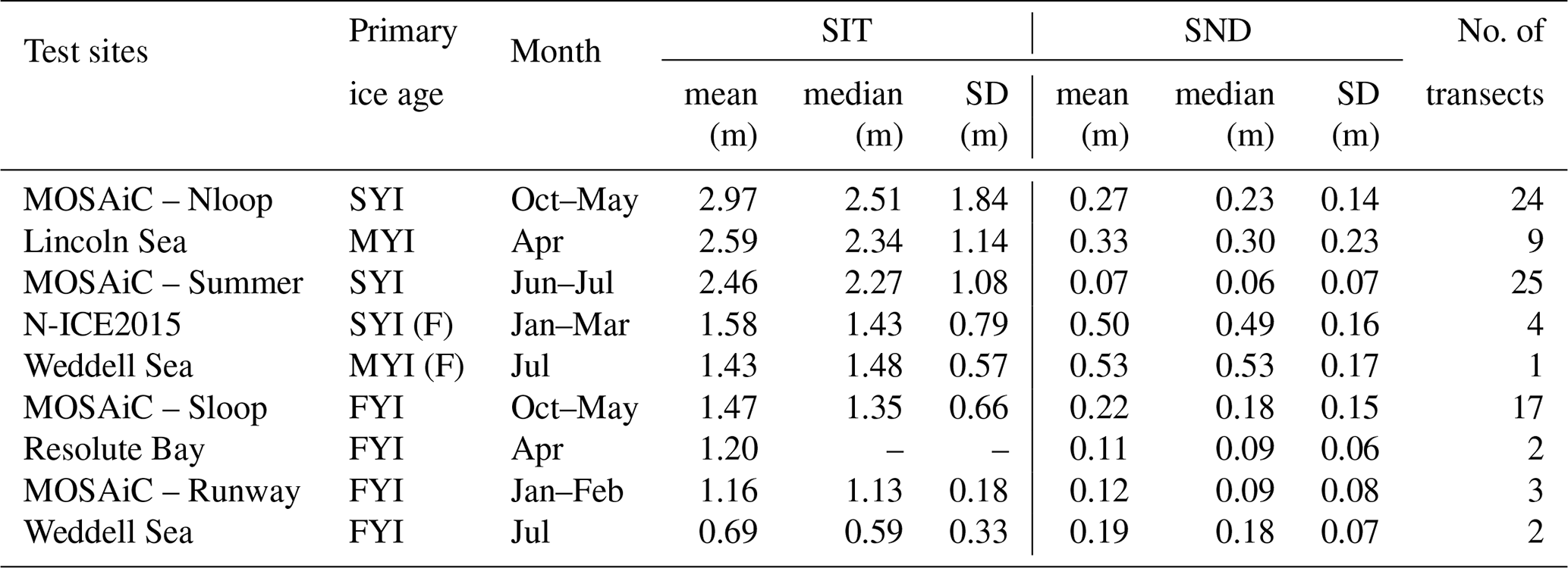
Based on the above criteria, the Multidisciplinary drifting Observatory for the Study of Arctic Climate (MOSAiC) 2019–2020 dataset was selected as the primary dataset because it spans a wide range of ice types and provides time-series in-situ measurements along repeated transects. The MOSAiC dataset includes four typical ice types: SYI and FYI from winter to spring, newly-formed smooth FYI in winter, and SYI in summer. Beyond MOSAiC, additional datasets were selected to capture two critical snow and ice conditions that are not represented in MOSAiC. First, to better account for the effects of thick snow on sea ice prone to flooding, we included data from the Norwegian Young Sea ICE Expedition 2015 (N-ICE2015) and the Weddell Sea (2013) campaigns. Second, the Lincoln Sea (2017) campaign was included to represent a distinct rough MYI type, enabling a more comprehensive assessment of SND distributions across different ice ages. We note that only three transects were acquired over newly-formed smooth FYI from the MOSAiC (i.e. Runway), as this site was disrupted by ice motion (Itkin and Liston, 2025). To improve sampling for this ice type, we included the Resolute Bay (2025) dataset, which represents smooth FYI covered by a thin snow layer comparable to that on the MOSAiC Runway. Although co-located SIT measurements were not available for Resolute Bay, field drilling indicated similar ice conditions (see Table 1). The geolocations of the selected test sites are shown in Fig. 1. Table 1 summarizes the ice type, season, mean, median, and standard deviation of both SIT and SND, and the number of transects, providing an overview of snow and ice properties of the selected test sites.

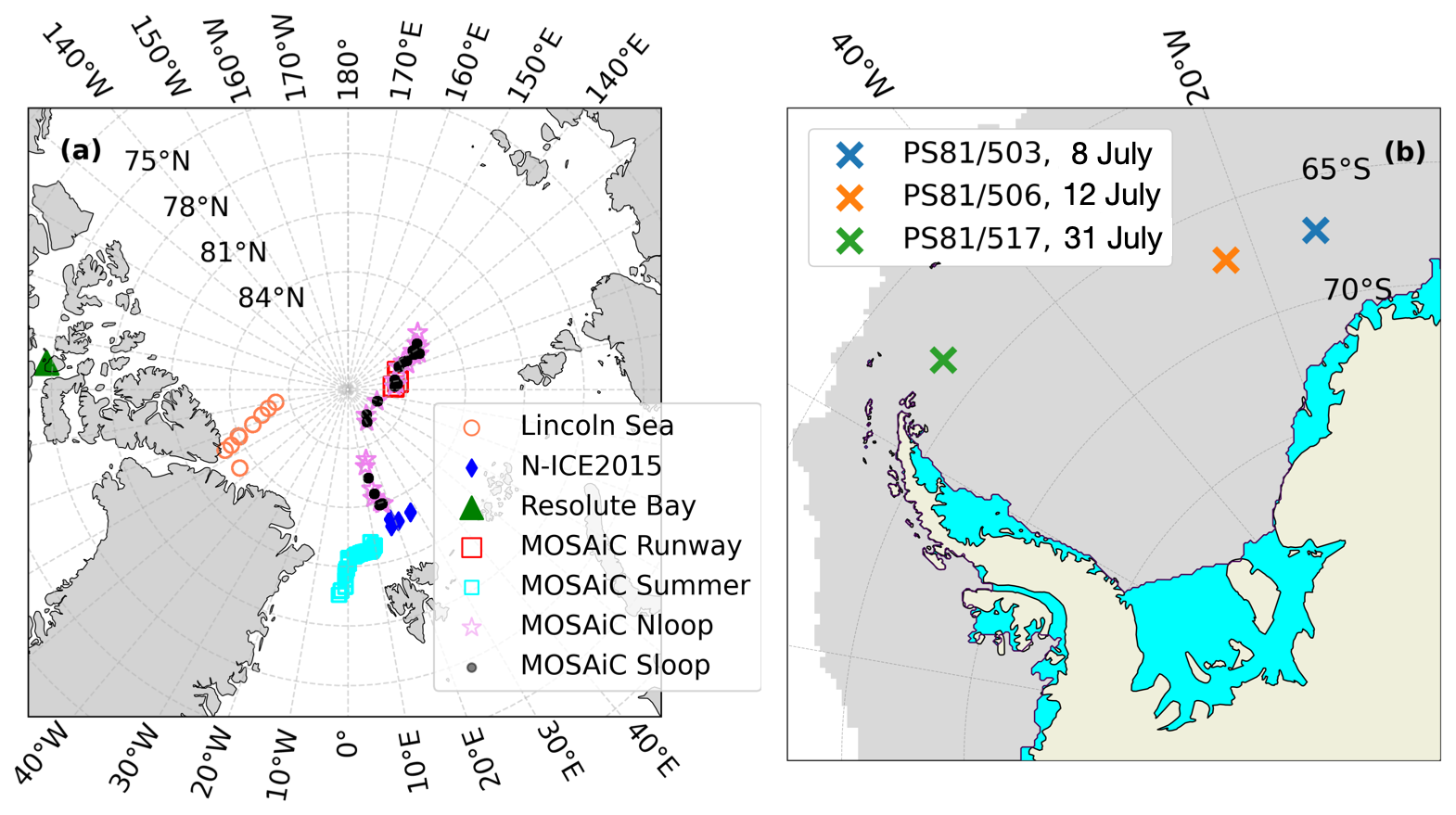
Figure 1 Geolocations of the selected field campaigns in the (a) Arctic and (b) Antarctic. In (a), MOSAiC Nloop and Sloop denote test sites of the MOSAiC northern and southern loops, respectively. (b) Data from the Weddell Sea survey in July 2013 (Lemke, 2014). The data are from the three ice stations: PS81/503, PS81/506 and PS81/517. Grey shading indicates sea ice cover on 31 July 2013 based on the NSIDC Bootstrap Sea Ice Concentration dataset (Comiso, 2023). Blue areas represent ice shelves derived from the NSIDC EASE-Grid 2.0 Land–Ocean–Coastline–Ice Masks dataset (Meier and Stewart, 2023).

2.2 Instruments

In all campaigns, SND measurements were carried out using automated snow-depth probes (magnaprobes) equipped with a data logger and GPS (Sturm and Holmgren, 2018). The device has a maximum measurement depth of 1.2 m, with an estimated accuracy of ∼3 mm (Sturm et al., 2006). In the Lincoln Sea, MOSAiC, and Weddell Sea campaigns, total thickness (snow + ice thickness) was sampled using a ground-based electromagnetic (EM) induction sounding system (GEM-2, Geophex Ltd.) operating at multiple frequencies (Hunkeler et al., 2015, 2016). During the N-ICE2015 campaign, total thickness was measured with portable EM instruments (EM31 and EM31SH, Geonics Ltd.) mounted on a sledge (Rösel et al., 2016a). The precision of the EM measurements is approximately 0.1 m on level ice up to 4 m thick. The accuracy decreases on rough and deformed ice, and the EM instrument can underestimate the ridge thickness by up to 50 % (Haas et al., 2009). For all datasets, SND and total thickness measurements were acquired along the same tracks.

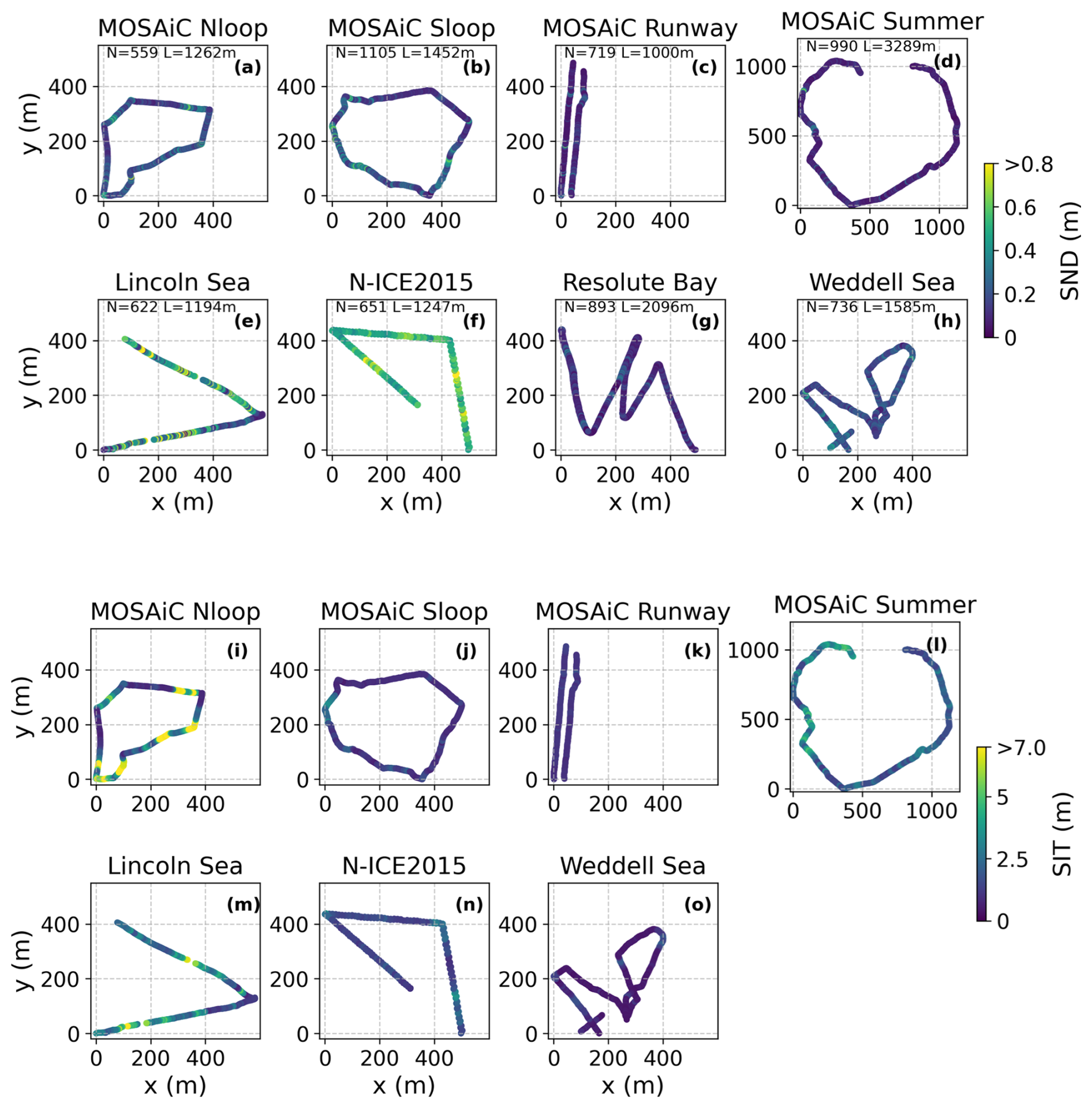
Figure 2 Examples of transects of snow depth (SND) and sea ice thickness (SIT) measurements. N is the total number of measurements and L is the total length of the transect. (a, i) MOSAiC northern loop (Nloop) transect on 14 November 2019. (b, j) MOSAiC southern loop (Sloop) transect on 26 December 2019. (c, k) MOSAiC Runway transect on 12 January 2020. (d, l) MOSAiC Summer transect on 3 July 2020. (e, m) Lincoln Sea 2017, transect 1. (f, n) N-ICE2015 transect on 28 January 2015. (g, o) Resolute Bay transect on 4 April 2025. (h, p) Weddell Sea, transect from floe 506. The x and y coordinates are shown as relative coordinates, with the bottom-left corner as the origin. The upper limit of the colorbar is set to the 99th percentile of the SND/SIT values.

All datasets had previously been corrected for sea ice drift following the procedures described in Itkin et al. (2023), Haas et al. (2017), Wever et al. (2021a), Merkouriadi et al. (2017). Co-location between magnaprobe and EM measurements was performed using nearest-neighbour interpolation. The co-location mismatch arises from the spacing between the magnoprobe and EM measurements, which is around 1–5 m (Merkouriadi et al., 2017; Haas et al., 2017; Wever et al., 2021a; Itkin et al., 2023). Given that our analyses in the following sections are based on values averaged along the transect rather than on individual measurements, the metre-scale mismatch is unlikely to influence the results. The SIT was then calculated as the co-located total thickness minus SND. Examples of the co-located SND and SIT along the transects are shown in Fig. 2.

2.3 In-situ measurements

Figure 3 shows an overview of the statistical distributions of SND and SIT measurements for each test site. Each test site comprises several sampling transects, and the corresponding violin plots for individual transects are provided in the Supplement (Figs. S1–S3).

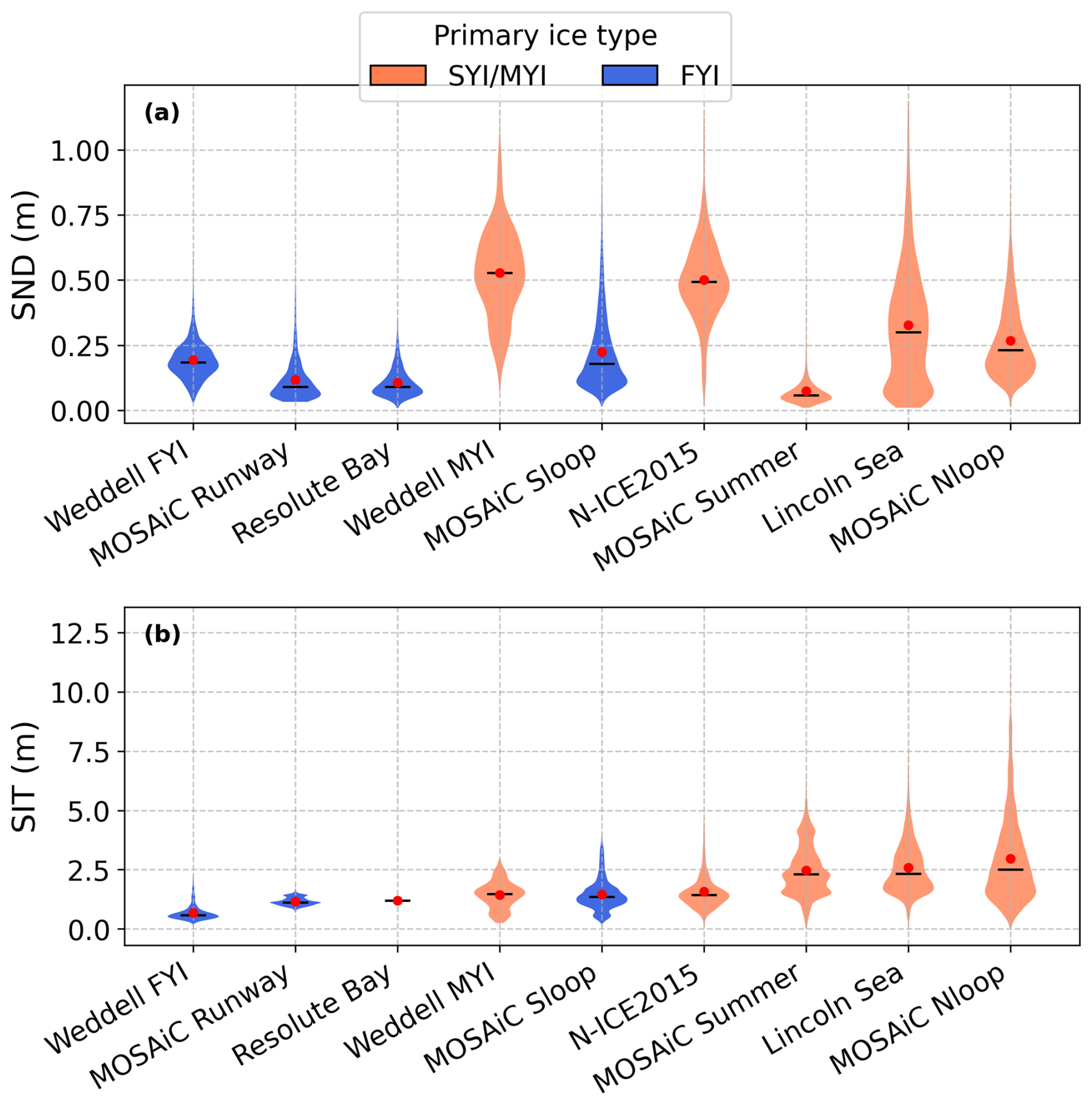
Figure 3 Violin plots of (a) snow depth (SND) and (b) sea ice thickness (SIT) for each study area, ranked in order of mean SIT. The red dot and black line represent the mean and median values, respectively.

2.3.1 MOSAiC 2019-2020

During MOSAiC, SND and total thickness were measured weekly over transects under various ice conditions (Nicolaus et al., 2022; Itkin et al., 2023). The EM 18 kHz measurements for total thickness are used in this study due to their higher signal-to-noise ratio (Itkin et al., 2023). The sites included the Northern Loop (Nloop), Southern Loop (Sloop), and Runway during the winter to spring season (24 October 2019–7 May 2020), as well as the Summer site from 17 June 2020 to 26 July 2020. The geolocation of these sites is shown in Fig. 1a. The GPS coordinates of the magnaprobe and EM measurements were converted to a local metric coordinate system (Itkin et al., 2023), with the ship position as the origin, using the FloeNavi toolbox (Hendricks, 2022).

A total of around 68 000 co-located magnaprobe and EM measurements were collected across the Nloop, Sloop, Runway, and Summer sites, at a spacing of 1–3 m (Itkin et al., 2021). The Nloop and Sloop sites each covered an area of ∼400 m × 400 m. The Runway site was located within a ∼100 m × 400 m area. The Summer site was located within an area of ∼1000 m × 1000 m. The MOSAiC Nloop was mainly deformed SYI, where the ice was older and thicker compared to other sites (Nicolaus et al., 2022; Wagner et al., 2022; Itkin et al., 2023). During the winter to spring season, the mean SIT was 2.97 m with mean SND values of 0.27 m. The MOSAiC Sloop, consisting primarily of FYI and remnant SYI, covered underlying frozen melt ponds and thus represents a younger and thinner ice section compared to the Nloop (Nicolaus et al., 2022; Wagner et al., 2022; Itkin et al., 2023). The mean SIT and SND were 1.47 and 0.22 m, respectively. The MOSAiC Runway was predominantly level FYI beginning at 0.05 m SIT on 20 October (Itkin and Liston, 2025). The formation of FYI on the Runway was observed by panoramic photography (Itkin et al., 2023) and was sampled three times in January and February 2020 until it was destroyed by ice motion. The Runway exhibited smooth and thin ice conditions, with a mean SIT and SND of 1.16 and 0.12 m, respectively. The MOSAiC Summer sites consisted predominantly of SYI, with a small spatial overlap with the Nloop site, while the last third of the transect was on FYI (Webster et al., 2022). The Summer site had a mean SIT of 2.46 m, while the snow layer was very thin (mean of 0.07 m). Detailed SND and SIT values along each transect are shown in the Supplement (Figs. S1–S2).

2.3.2 Resolute Bay 2025

A recent fieldwork was conducted at two different locations of landfast ice (4 and 6 April 2025) in Resolute Bay, Qikiqtaaluk Region, Nunavut, Canada (Fig. 1a). This dataset represents smooth FYI covered by a thin and smooth snow layer. No new snowfall occurred during the sampling period (Stroeve et al., 2026).

A total of around 1560 magnaprobe samples were collected along two transects, at a sampling spacing of 1–4 m. Each transect covered an area of approximately 300 m × 500 m. The two transects had similar mean SND values of 0.11 m. The transect on 6 April was observed to be smoother than the one on 4 April (Stroeve et al., 2026). The snow statistics (mean and standard deviation) are similar to those of the MOSAiC Runway dataset (Table 1), thereby providing a useful complement given that the MOSAiC Runway includes only three transects. Among all sites, Resolute Bay and the MOSAiC Runway exhibit the lowest mean and standard deviation of SND. Note that no coincident SIT measurements were available for individual SND samples; however, ice drilling indicated a SIT of approximately 1.2 m.

2.3.3 Lincoln Sea 2017

From 11 to 18 April 2017, co-located SND and SIT measurements were collected as part of the ESA CryoSat-2 Validation Experiment (CryoVEx) 2017 campaign, including nine transects between Ellesmere Island and 86.3° N (Fig. 1a). During the campaign, the sampling locations were covered by thick and deformed fast ice as well as drift MYI floes and SYI. The Lincoln Sea site captures a clear trend of decreasing SIT and ice age from the south to the north: thick and deformed landfast ice (transects 1–5), followed by drift sea ice with mixed MYI and SYI (transects 6–8), and finally a mixture of SYI and thick FYI (transect 9) (Haas et al., 2017). The transect numbers are shown later in Fig. 10.

A total of around 6400 co-located magnaprobe and EM measurements were collected at nine transects, at a spacing of 1–5 m (Haas et al., 2017). It comprises seven transects within an area of 500 m × 1000 m, and two transects slightly above the sub-kilometre scale (i.e. 900 m × 1600 m and 1100 m × 1400 m for transects 5 and 6, respectively). The site had a mean SIT of 2.59 m and a mean SND of 0.33 m, see Table 1 and Fig. 3. Detailed SND and SIT observations along each transect are shown in the Supplement (Fig. S3).

2.3.4 N-ICE2015

The N-ICE2015 expedition took place from January to June 2015 aboard the Norwegian R/V Lance research vessel north of Svalbard. During the campaign, Lance served as a research platform, moored to a sea ice floe, and moving with the sea ice drift. This study uses repeat transect data from the winter part of the N-ICE2015 campaign (22 January–15 March 2015), which represent SYI with significant snow load (Merkouriadi et al., 2017). The coincident SND and SIT measurements were from Floe 1 (28 January and 7 February 2015) and Floe 2 (28 February and 14 March 2015) (Rösel et al., 2016a, b). Both floes were situated in ice packs primarily composed of SYI (Granskog et al., 2018), with the snow stratigraphy on Floe 1 showing more wind slabs than Floe 2 (Merkouriadi et al., 2017). The geolocation of the four transects is shown in Fig. 1a.

A total of around 2130 co-located magnaprobe and EM31 measurements were collected across two repeat transects, at a spacing of 1–5 m. Each transect was within an area of 600 m × 1000 m. Across the two repeat transects, the mean SIT was 1.58 m covered by thick snow layers with a mean of 0.5 m, as shown in Table 1 and Fig. 3. Detailed SND and SIT values along each transect are shown in the Supplement (Fig. S3). Note that during the N-ICE2015 expedition, widespread negative freeboard and snowpack flooding were observed, resulting from thick snow over relatively thin sea ice (Merkouriadi et al., 2017; Rösel et al., 2021). Specifically, flooding was observed in 3 of the 10 drill holes (Rösel et al., 2021).

2.3.5 Weddell Sea 2013

To ensure a sufficient representation of thick snow conditions comparable to N-ICE2015 (two repeat transects), we included data from the Antarctic Winter Ecosystem and Climate Study (AWECS, ANT-XXIX/6), which surveyed the Weddell Sea between June and August 2013 (Lemke, 2014). During the campaign, SND and SIT measurements were collected from three ice floes: PS81/503 on 8 July 2013, PS81/506 on 12 July 2013, and PS81/517 on 31 July 2013, hereafter referred to as floe 503, 506, and 517. Floes 503 and 506 were FYI, while floe 517 was MYI (Arndt and Paul, 2018; Wever et al., 2021b). The locations of the floes are shown in Fig. 1b.

A total of around 1720 co-located magnaprobe and EM measurements were collected over three floes, at a spacing of 1–5 m. Each transect was within an area of approximately 400 m × 400 m. For FYI floes (503 and 506), the mean SIT and SND were 0.69 and 0.19 m, respectively. For MYI floe (517), the mean SIT and SND were 1.43 and 0.53 m, respectively, shown in Table 1 and Fig. 3. The detailed SND and SIT observations along each transect are shown in the Supplement (Fig. S3). Note that during the campaign, drilling measurements occasionally indicated negative freeboards for floes 506 and 517, with a median freeboard of 0 m, suggesting that both floes were susceptible to flooding (Wever et al., 2021a). The snowpacks on the Weddell Sea MYI floe 517 and during the N-ICE2015 field campaign are the thickest snowpacks in this study.

3 Methods

3.1 Statistical distributions

This section introduces four statistical distributions for fitting the observed SND samples: normal, log-normal, gamma, and skew. For a normal distribution with mean μ_g and standard deviation σ_g, the PDF is given by

$$\begin{array}{}\text{(1)}& N(x;{\mathit{\mu }}_{\mathrm{g}},{\mathit{\sigma }}_{\mathrm{g}})={\displaystyle \frac{\mathrm{1}}{\sqrt{\mathrm{2}\mathit{\pi }{\mathit{\sigma }}_{\mathrm{g}}^{\mathrm{2}}}}}{e}^{-\frac{(x-{\mathit{\mu }}_{\mathrm{g}}{)}^{\mathrm{2}}}{\mathrm{2}{\mathit{\sigma }}_{\mathrm{g}}^{\mathrm{2}}}}\end{array}$$

The PDF of the log-normal distribution follows (Gaddum, 1945):

$$\begin{array}{}\text{(2)}& \text{LG}(x;{\mathit{\mu }}_{\mathrm{l}},{\mathit{\sigma }}_{\mathrm{l}})={\displaystyle \frac{\mathrm{1}}{x{\mathit{\sigma }}_{\mathrm{l}}\sqrt{\mathrm{2}\mathit{\pi }}}}{e}^{-\frac{\left(\ln \right(x)-{\mathit{\mu }}_{\mathrm{l}}{)}^{\mathrm{2}}}{\mathrm{2}{\mathit{\sigma }}_{\mathrm{l}}^{\mathrm{2}}}}\end{array}$$

where μ_l and σ_l are the location and scale parameters in the logarithmic space, respectively. The mean and variance are $e^{({\mathit{\mu }}_{\mathrm{l}}+{{\mathit{\sigma }}_{\mathrm{l}}}^{\mathrm{2}}/\mathrm{2})}$ and $e^{\mathrm{2}{\mathit{\mu }}_{\mathrm{l}}+{\mathit{\sigma }}_{\mathrm{l}}^{\mathrm{2}}}\left(e^{{\mathit{\sigma }}_{\mathrm{l}}^{\mathrm{2}}}-\mathrm{1}\right)$, respectively.

The PDF of the gamma distribution is defined as (Thom, 1958):

$$\begin{array}{}\text{(3)}& \text{Ga}(x;a_{\mathrm{g}},\mathit{\theta })={\displaystyle \frac{\mathrm{1}}{\mathrm{\Gamma }\left(a_{\mathrm{g}}\right){\mathit{\theta }}^{a_{\mathrm{g}}}}}{x}^{a_{\mathrm{g}}-\mathrm{1}}{e}^{-x/\mathit{\theta }}\end{array}$$

where a_g>0 is the shape parameter and θ>0 is the scale parameter. Γ(⋅) is the gamma function.

The PDF of the skew distribution with standard deviation σ_s is given as (O'Hagan and Leonard, 1976; Azzalini and Capitanio, 2002):

$$\begin{array}{}\text{(4)}& \begin{array}{rl}S({\mathit{\sigma }}_{\mathrm{s}};\mathit{\omega },a_{\mathrm{s}},\mathit{\xi })& ={\displaystyle \frac{\mathrm{1}}{\mathit{\omega }\sqrt{\mathrm{2}\mathit{\pi }}}}\left(\mathrm{1}+\text{erf}\left({\displaystyle \frac{a_{\mathrm{s}}x}{\sqrt{\mathrm{2}}}}\right)\right)e^{-(x^{\mathrm{2}}/\mathrm{2})},\\ x& ={\displaystyle \frac{{\mathit{\sigma }}_{\mathrm{s}}-\mathit{\xi }}{\mathit{\omega }}}\end{array}\end{array}$$

where ω is the scaling parameter, a_s is the shape parameter, ξ is the location parameter, and erf(⋅) is the error function.

The four PDFs are used to fit the observed SND distributions. For each transect, the PDF parameters for each distribution are estimated using maximum likelihood estimation (MLE) (Myung, 2003). Considering that each transect has hundreds of samples, overfitting of MLE can be negligible. Figure 4a shows an example transect from MOSAiC Nloop (14 November 2019), where the histogram of the observed SND is shown as a step-line plot, while the fitted distributions are displayed in different colours.

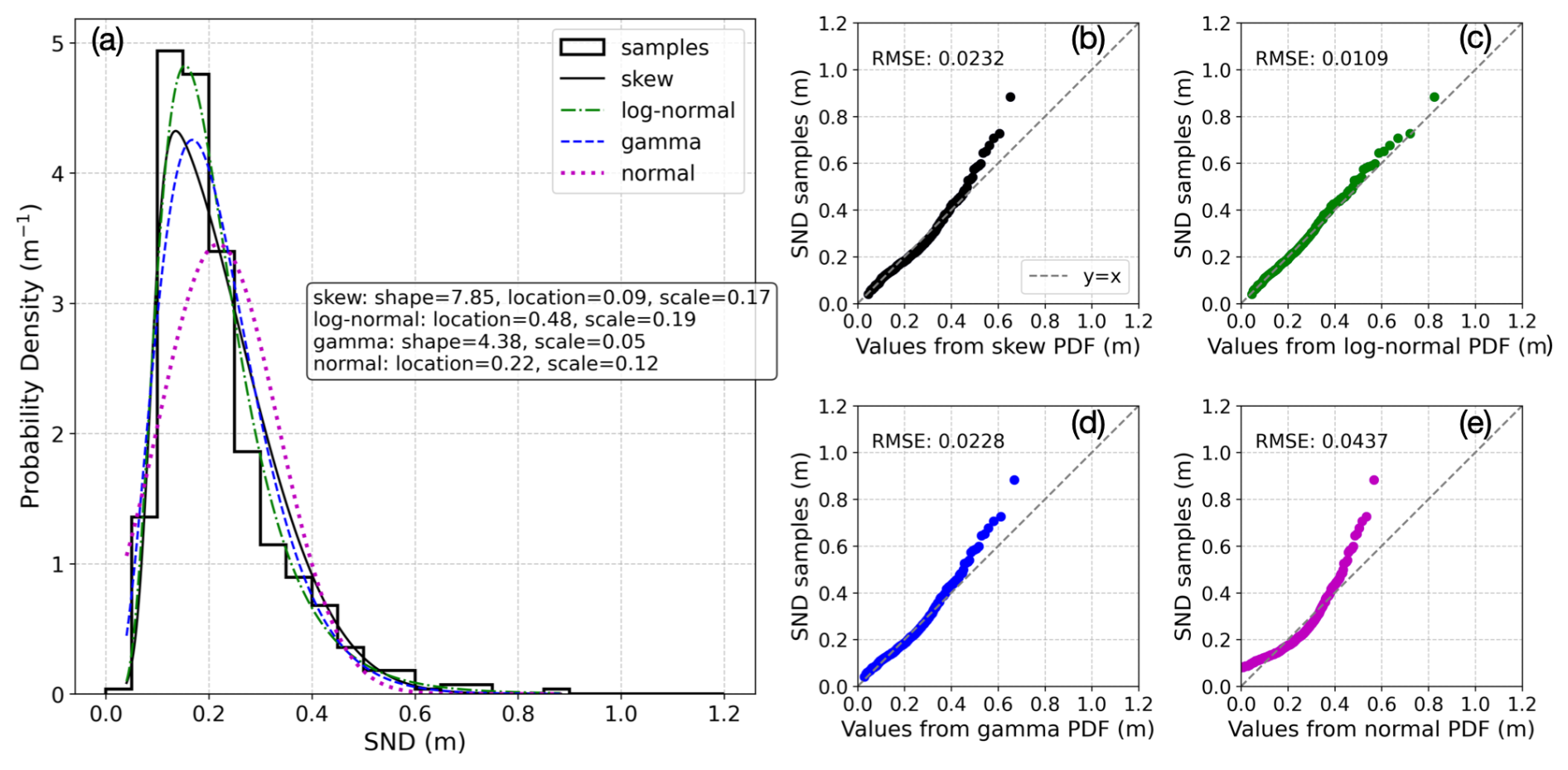
Figure 4 (a) Comparison of the skew, log-normal, gamma, and normal probability density functions (PDFs) with the histogram of measured snow depth (SND) values of a transect from MOSAiC northern loop (Nloop) on 14 November 2019. The histogram is generated with a bin width of 5 cm. (b–e) Quantile-quantile (Q-Q) plots illustrate the goodness of fit. The root-mean-squared error (RMSE) between the fitted distribution and the observed SND quantiles is calculated to quantify the goodness of fit. The black dashed lines in (b)–(e) are the 1:1 lines.

The goodness of fit is assessed using a quantile-quantile (Q-Q) plot, which compares the quantiles of the observed SND values with those of the fitted distributions (Wilk and Gnanadesikan, 1968). If the fitted distribution accurately represents the data, the points in the Q-Q plot should be along the 1:1 line. Deviations from this line indicate discrepancies between the observed and fitted distributions. To quantify the goodness of fit, we calculate the root-mean-square error (RMSE) between the observed and fitted quantiles (Wilk and Gnanadesikan, 1968):

$$\begin{array}{}\text{(5)}& \text{RMSE}=\sqrt{{\displaystyle \frac{\mathrm{1}}{n}}\sum _{i=\mathrm{1}}^n{\left(Q_{\mathrm{obs},i}-Q_{\mathrm{fit},i}\right)}^{\mathrm{2}}}\end{array}$$

where Q_obs,i and Q_fit,i are the ith quantiles of the observed and fitted distributions (Fig. 4b–e), respectively, and n is the total number of quantile points considered. A lower RMSE indicates a better fit. In contrast to the histogram, which is sensitive to arbitrary binning choice, the Q-Q plot enables a direct quantile–quantile comparison between the observed and theoretical distribution. Consequently, the RMSE derived from the Q-Q plot is not affected by binning, providing a more objective basis for evaluating model performance.

3.2 Geostatistics and variogram

Spatial variability in SND is controlled by factors such as local precipitation, wind redistribution, ice topography, and the amount of snow already accumulated in pre-existing bedforms that can be reworked by wind (Moon et al., 2019). A variogram provides a measure of the spatial continuity of snow cover and how it varies with distance and orientation on sea ice (Iacozza and Barber, 1999). A variogram can be computed by relating the semi-variance γ(h) to the lag distance (Sturm et al., 1995):

$$\begin{array}{}\text{(6)}& \mathit{\gamma }\left(h\right)={\displaystyle \frac{\mathrm{1}}{\mathrm{2}N}}{\mathrm{\Sigma }}_{i=\mathrm{1}}^N(x_i-x_{i+h}{)}^{\mathrm{2}}\end{array}$$

where x_i and x_i+h are the sample values (measured SND) at the location i and i+h respectively. N denotes the number of observations at a specific lag distance h.

In this study, the semi-variogram analysis employs the Matheron estimator (Matheron, 1962) with an exponential model and incorporates a non-zero nugget effect, using a bin width of 3 m. The non-zero nugget reflects either measurement error or spatial variability occurring at scales smaller than the 3 m bin size (Filhol and Sturm, 2015). Note that the bin width is set to 3 m based on the median spacing of the magnaprobe measurements. This choice ensures sufficient point pairs per bin while resolving spatial variability up to the sill. A constant bin width of 3 m enables a consistent comparison of variogram parameters across sites. We adopt the exponential model to fit the semi-variogram, as it provides a good balance between simplicity and accuracy. Data screening and data quality are essential for semi-variogram analyses. In this study, measurements with distances greater than 10 m are excluded, as they correspond to periods when the magnaprobe was moved between sampling locations. In addition, measurements with snow depths <1 cm or equal to 120 cm (the operational limits of the magnaprobe) were removed.

Figure 5 presents the semi-variogram of SND measurements collected from MOSAiC Sloop transect on 14 November 2019, as an example. The fitted exponential model approaches the sill, and the effective range corresponds to the lag distance where the modeled semi-variance reaches 95 % of the sill value. In the following, this effective range is referred to as the correlation length. The snow correlation length is the distance over which the SND remains spatially correlated; beyond this scale, the measurements become effectively independent. The correlation length provides a statistical measure of spatial continuity. Larger correlation lengths can be associated with prominent surface features, such as ridges and snow dunes, which can extend up to tens of meters (Filhol and Sturm, 2015). The estimated correlation length can be influenced by the spacing of the magnaprobe measurements. Finer sampling intervals allow the semi-variogram to resolve small-scale snow bedforms (Filhol and Sturm, 2015), whereas coarser spacing may miss these features and instead primarily capture broader-scale snow structures, leading to a longer apparent correlation length. Moon et al. (2019) showed that a characteristic scale of around 10 m is associated with the formation of snow dunes, whereas a second scale, between 30 and 100 m, likely reflects interactions among dunes, such as merging, calving, and lateral linking.

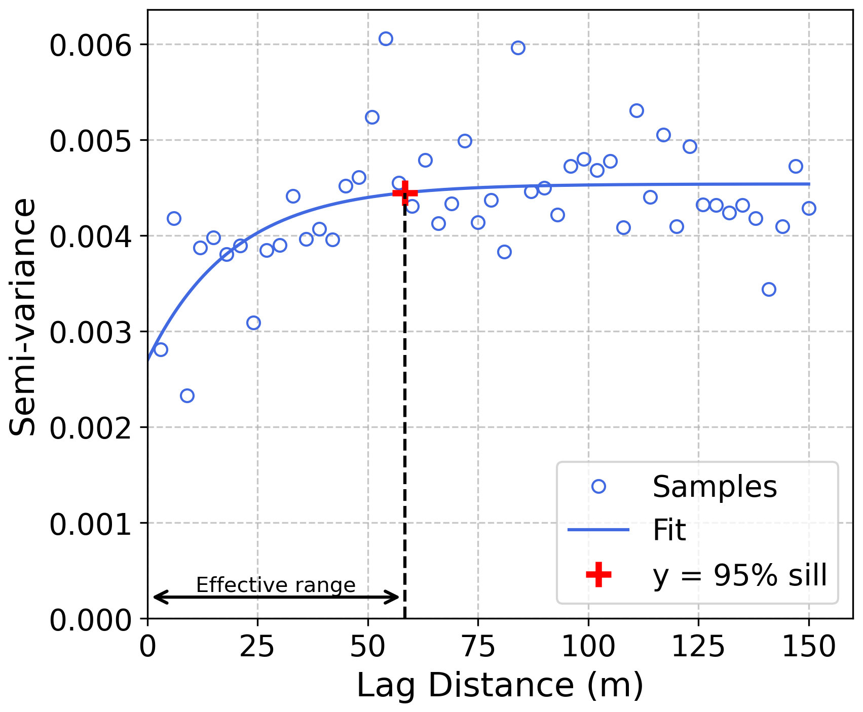
Figure 5 Semi-variogram of snow depth (SND) measurements collected on the MOSAiC southern loop (Sloop) on 14 November 2019.

4 Results

In this section, we first examine the statistical properties of the SND distribution (mean and standard deviation) and their relationship to ice type and SIT. We then fit the SND observations using statistical PDFs and identify the most suitable model for different ice types. Finally, we estimate the SND correlation lengths from semi-variograms and analyse their relationship to SIT and meteorological events.

4.1 Statistical properties of snow depth

To examine the relationship between SND and SIT for different ice types, we calculated the mean (μ_SND) and standard deviation (σ_SND) of SND, as well as the mean SIT (μ_SIT) for each transect at each site, as shown in Fig. 6. A clear linear relationship is observed between μ_SND and μ_SIT for FYI. This can be explained by the concurrent increase in SND and SIT during the ice thermodynamic growth season. In contrast, no significant linear relationship is observed for SYI and MYI. For these ice types, SIT is no longer controlled primarily by ongoing thermodynamic growth, as they tend to approach a quasi-equilibrium thickness. At the same time, the overlying snow has a longer residence time and is therefore increasingly modified by post-depositional processes such as wind-driven redistribution and the influence of surface roughness, rather than by concurrent snow accumulation alone.

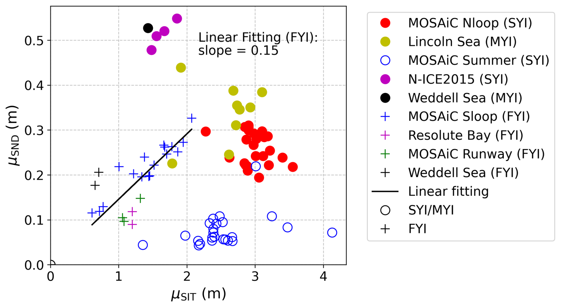
Figure 6 The relationship between the snow depth (SND) and sea ice thickness (SIT), where μ_SND and μ_SIT denote the mean SND and mean SIT values of each transect, respectively. The colour and symbol (“∘” and “+”) represent different test sites and ice types, respectively.

Since CV is defined as the ratio of σ_SND to μ_SND, a linear relationship is expected (Brown, 1998):

$$\begin{array}{}\text{(7)}& {\mathit{\sigma }}_{\mathrm{SND}}=\mathrm{CV}\times {\mathit{\mu }}_{\mathrm{SND}}\end{array}$$

which suggests that σ_SND can be estimated when μ_SND is known.

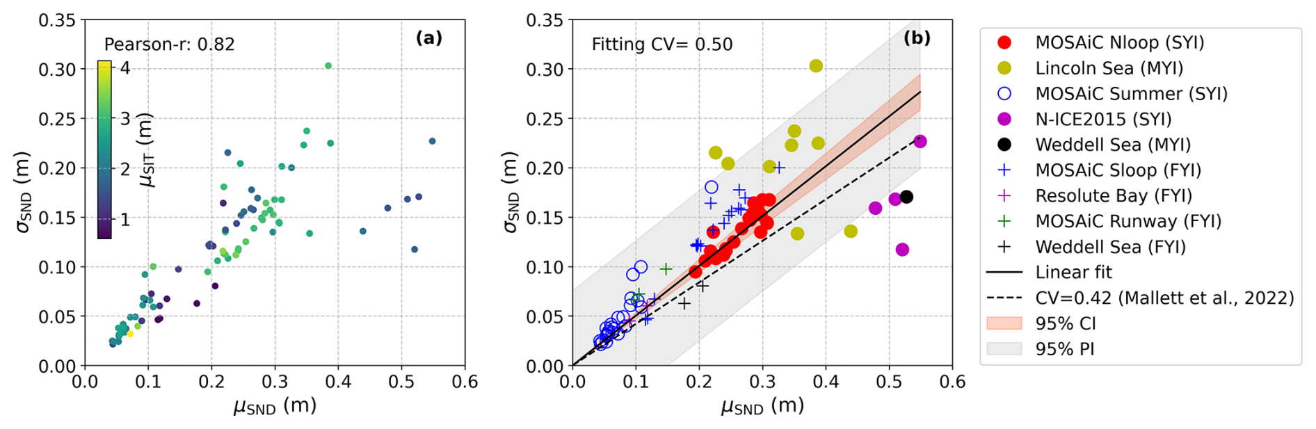
Figure 7 Relationship between each transect's average snow depth (SND, μ_SND) and the corresponding standard deviation (σ_SND). (a) The colour represents the mean ice thickness (SIT) of each transect. (b) The colour and symbol (“∘” and “+”) represent different test sites and ice types, respectively. The 95 % confidence interval (CI) and 95 % prediction interval (PI) are plotted in coral and gray shade. The coefficient of variation (CV = ${\mathit{\sigma }}_{\mathrm{SND}}/{\mathit{\mu }}_{\mathrm{SND}}$) is calculated by linear fitting.

Figure 7a shows the relationship between σ_SND and μ_SND for all sites. The results do not show a dependence of CV on μ_SIT, suggesting a constant value of CV across different ice types. A linear fit between σ_SND and μ_SND in Fig. 7b gives CV=0.5. The CV can be used to estimate SND variability from its mean value, as obtained from snow modelling (Liston et al., 2020). Most of the Lincoln Sea samples lie above the fitted line, indicating enhanced SND variability which can be linked to observed ice rafting events and significantly deformed surfaces. In contrast, samples from N-ICE2015 and the Weddell Sea (MYI) fall below the fitted line, with lower CV values than the other sites. Interestingly, these two sites experienced flooding (Merkouriadi et al., 2017; Rösel et al., 2021; Wever et al., 2021a). Flooding wets the basal snow layer, promoting wet-snow settling and densification that reduce the mean SND (Colbeck, 1979; Marshall et al., 1999; Techel et al., 2008; Wever et al., 2021a). Although flooding reduces mean SND, it is also associated with a lower-than-expected variability, leading to a reduced CV.

The reduced SND variability at flooded sites may arise from two physical mechanisms. First, because overburden stress increases with SND, thicker snow can undergo greater compaction once wet (Colbeck, 1979; Marshall et al., 1999), leading to a greater reduction in SND than thinner snow and thus reducing spatial SND variability. Mallett et al. (2024) reported the lowest brine wicking in the lowest-density layer, while the denser layers tended to exhibit higher wicking heights. A plausible explanation is that smaller capillaries in denser basal snow increase capillary suction, enhancing upward brine infiltration and increasing the volume of snow that becomes slush and subsequently freezes into snow ice. If snow-ice formation is more extensive in initially thicker snow, this could amplify net snow-thickness loss there and further suppress spatial SND variability. Second, snow may become more cohesive and mechanically stronger after flooding, making it less susceptible to wind-driven redistribution. In winter, upward conductive heat flux from the ocean warms the ice–snow interface, increasing the temperature gradient across the snow (for a given air temperature) and also raising the snow's mean temperature. Since sintering accelerates at higher temperatures (Blackford, 2007; Clemens-Sewall et al., 2022), snow warmed by basal flooding sinters faster, thus increasing cohesion and making the snow less susceptible to wind redistribution and thus reducing SND variability. The difference in CV between flooded and non-flooded sites suggests that flooding can imprint a measurable signature in the SND distribution. The above proposed mechanisms still require validation through sufficient in-situ SND and SIT measurements at flooded sites.

4.2 Snow depth variability through distribution fitting

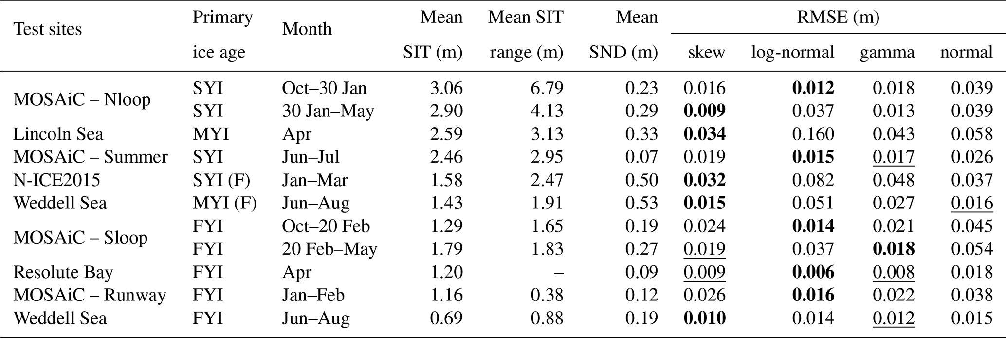
This subsection investigates (1) temporal variability based on the MOSAiC datasets; (2) the dependence of PDF fitting performance on ice age and SIT across all test sites. Following the method introduced in Sect. 3.1, the observed SND values for each transect across the test sites are fitted using the four probability distributions: normal, log-normal, gamma, and skew. The corresponding RMSE values derived from Q-Q plots are calculated to identify the most appropriate distribution for each sub-kilometre-scale transect (summarized in Table 2). To capture the levels of deformation, we define the SIT range (Δ_SIT) as the difference between the 95th and 5th percentiles of SIT for each transect.

Table 2 Performance of probability density function (PDF) fitting for snow depth (SND) across all sites. The root-mean-square error (RMSE) values measure the goodness of fit. The mean of sea ice thickness (SIT) and SND are calculated over all the transects for each site (row). Mean SIT range refers to the difference between the 95th and 5th percentiles of SIT for all transects within the site. The best-performing PDF (i.e. smallest RMSE value) is in bold. RMSE values that are underlined indicate PDFs for which the difference in RMSE is less than 0.003 m, corresponding to the instrumental precision of the magnaprobe. Ice types include first-year ice (FYI), second-year ice (SYI), and multi-year ice (MYI), with (F) denoting sites identified as susceptible to flooding.

4.2.1 Temporal variability

To enable effective time-series analysis of PDF fitting performance, we selected repeated measurements collected along the same transects from the MOSAiC dataset. The names of the transects used in this study are listed in the Supplement (Table S1). The fitting performances (i.e. RMSE values) of MOSAiC Nloop, Sloop, Runway, and Summer sites are shown in Figs. 8–9. Skewness and kurtosis values are provided to interpret the fitting performance. Kurtosis describes the tailedness of a distribution; lower kurtosis indicates a flatter distribution with fewer extreme values and more observations concentrated around the mean. Skewness quantifies the degree of asymmetry of a distribution; positive skewness indicates a longer right tail, whereas negative skewness indicates a longer left tail. The meteorological events reported in Wagner et al. (2022) are indicated in Fig. 8. Storms were closely related to ice deformation events. The first major change in ice conditions occurred around 16 November 2019, when a storm triggered strong ice deformation near the observation site. Another significant ice deformation event occurred around 11–12 March 2020 and periodically until 7 May 2020 (Wagner et al., 2022). Drifting snow events were identified by calculating the horizontal mass flux from snow particle counter (SPC) measurements. During periods of instrument downtime, a critical friction velocity threshold was applied to infer potential snow transport. The most significant drifting snow event occurred on 24–25 February 2020, during which the lower SPC recorded a cumulative mass flux of $\mathrm{1.014}\times {\mathrm{10}}^{\mathrm{6}}\mathrm{kg}{\mathrm{m}}^{-\mathrm{2}}$. During this event, 1 h average wind speeds at 2 m above the ice reached approximately 11 m s⁻¹, with instantaneous wind speeds at shorter temporal scales likely exceeding this value (Wagner et al., 2022).

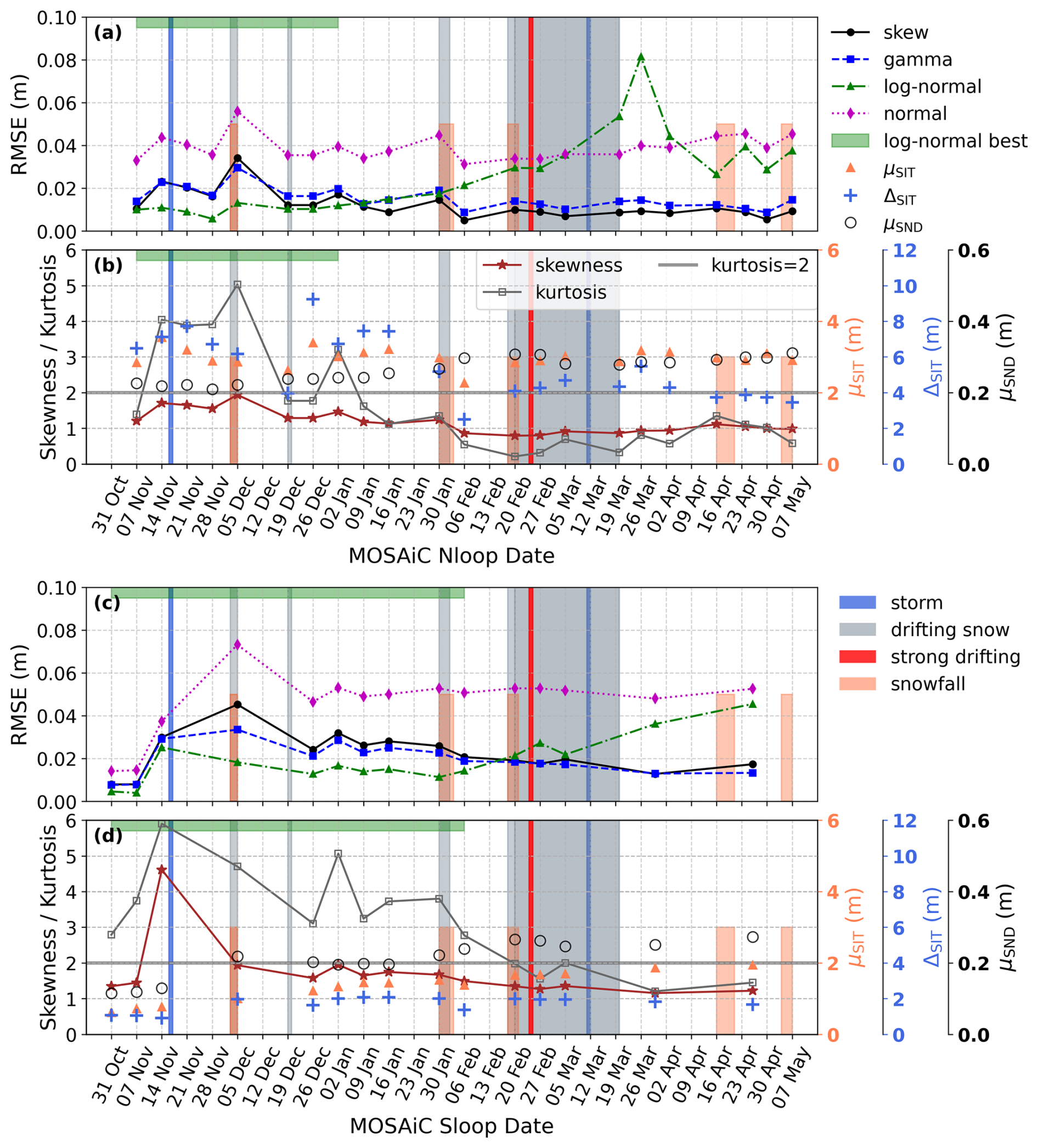
Figure 8 Time-series analyses of snow depth (SND) distribution over MOSAiC northern loop (Nloop) (a–b) and southern loop (Sloop) (c–d). The relevant meteorological events such as storm, snowfall, and drifting snow are from Wagner et al. (2022). (a) and (c) are root-mean-square error (RMSE) between the fitted probability density functions (PDFs) and the measured SND values. The dates on which the log-normal performs best are marked by green bars. (b) and (d) show skewness and kurtosis values calculated from the measured SND values. The mean SND (μ_SND), mean sea ice thickness (SIT, μ_SIT), and SIT range (Δ_SIT=95 % SIT − 5 % SIT) of each transect are also plotted.

For the MOSAiC Nloop (Fig. 8a), we observe a temporal shift in the best-fitting distribution on 30 January 2020, with the log-normal performing best initially, followed by a transition to the skew distribution. Before 19 December 2019, the log-normal distribution (green line) provides the best fit to the observed SND, with the lowest RMSE compared to the other PDFs, as shown in Fig. 8a. Since 19 December 2019, the performances of gamma and skew improve, coincident with a notable drop in kurtosis values below 2, as shown in Fig. 8b. A possible explanation for this transition is the drifting snow events reported on 3–5 December and 19 December (Wagner et al., 2022), which can reduce the peakedness of the SND distribution and lead to a more evenly redistributed snow layer.

From 19 December 2019 to 30 January 2020 (Fig. 8a), the performance of the gamma (blue line) and skew (black line) distributions improves, reaching RMSE values at the same level as the log-normal distribution. We observe kurtosis<2 (Fig. 8b) on 9 January 2020, coincident with the point where the skew distribution begins to outperform the log-normal distribution. The dates on which the log-normal performs best are marked by green bars in Fig. 8, suggesting that kurtosis >2 can represent a threshold above which the log-normal distribution outperforms the skew distribution. This threshold is also supported at all other test sites. Note that kurtosis values are slightly below 2 on 7 November, 19 December, and 26 December 2019, when the log-normal distribution still yields the smallest RMSE. However, in these three cases, the RMSE differences between log-normal and skew distributions are less than 0.003 m, which is within the instrumental precision of the magnaprobe, suggesting that both distributions perform comparably well.

After 30 January 2020 (Fig. 8a), coincident with a drifting snow event, the performance of the log-normal distribution deteriorates continuously, as reflected by a continuous increase in RMSE; while the skew distribution achieves the best fit with the lowest RMSE. Log-normal performance continues to decline during the drifting snow period from 20 February to 20 March 2020, including the strong drifting snow on 24–25 February 2020. During this period, observed SND samples exhibit the lowest kurtosis (∼0.2–0.8). These observations indicate that wind-driven redistribution events, such as drifting snow, cause the SND distribution to deviate from log-normal behaviour and favour a skew distribution. It can be attributed to the fact that Nloop was sampled on thick and deformed SYI with pronounced ridges, as supported by the large SIT range reported in Table 2. Such deformed ice topography promotes a non-homogeneous SND distribution. The subsequent drifting snow event likely redistributed the snow, leading to a more homogeneous SND distribution and resulting in a distribution better described by the skew distribution.

For MOSAiC Sloop, where FYI dominates, the continuous increase in μ_SIT over time indicates seasonal thermodynamic growth of sea ice (Fig. 8c). Similarly to Nloop, a temporal shift in the best-fitting distribution can be observed on 20 February 2020, with the log-normal performing best initially, followed by a transition to the gamma/skew distribution. Before 20 February 2020, log-normal performs best, exhibiting the lowest RMSE values. Similarly to Nloop, a significant improvement in gamma and skew performance is observed on 26 December 2019, after a documented drifting snow event that occurred on 19 December 2019 (Wagner et al., 2022). After 20 February 2020, μ_SIT reaches approximately 1.5 m. The gamma and skew distributions begin to outperform the log-normal, with the gamma distribution performing slightly better than the skew distribution. From Fig. 8d, kurtosis decreases below the threshold of 2 since 20 February 2020, consistent with the transition of the best-fit PDF from log-normal to gamma or skew distribution. It supports the previous observation that kurtosis >2 can represent a threshold above which the log-normal distribution outperforms the skew distribution. The deterioration in log-normal performance after 20 February 2020 is also coincident with the drifting snow period beginning that day, further supporting the interpretation that the drifting snow event leads to more evenly redistributed snow layers as observed in the MOSAiC Nloop results. Notably, unlike the Nloop over SYI where μ_SIT remains relatively constant, the transition of the best-fitting PDF from log-normal to skew indicates a clear dependence of the SND distribution on SIT for FYI during the growth season. This relationship is further discussed in Sect. 4.2.3.

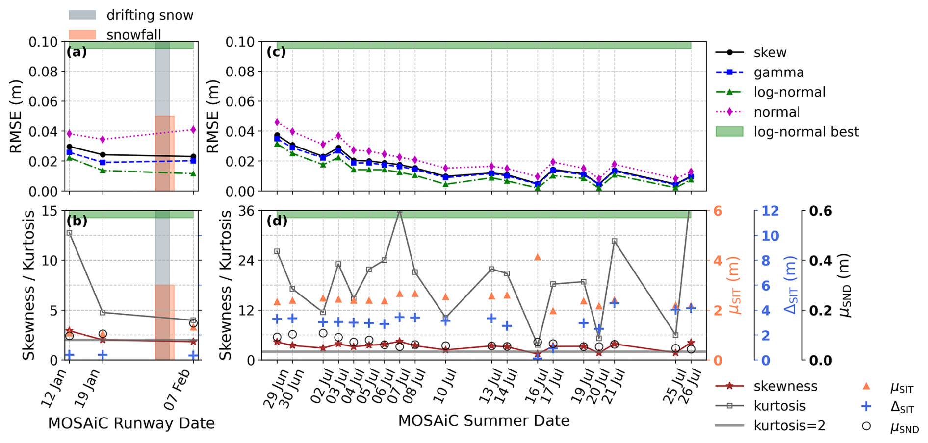
Figure 9 Time-series analyses of snow depth (SND) distribution over MOSAiC Runway (a–b) and MOSAiC Summer (c–d). (a) and (c) are root-mean-square error (RMSE) between the fitted probability density functions (PDFs) and the measured SND values. The dates on which the log-normal performs best are marked by green bars. (b) and (d) show skewness and kurtosis values calculated from the measured SND values. The mean SND (μ_SND), mean sea ice thickness (SIT, μ_SIT), and SIT range (${\mathrm{\Delta }}_{\mathrm{SIT}}=\mathrm{95}\mathit{\%}\mathrm{SIT}-\mathrm{5}\mathit{\%}\mathrm{SIT}$) of each transect are also plotted.

The MOSAiC Runway site was covered by newly-formed smooth FYI, with μ_SIT ranging between 1 and 1.3 m and a thinner snow layer (μ_SND from 0.1–0.15 m) compared to the MOSAiC Nloop and Sloop. In Fig. 9a, the log-normal provides the best fit of the observed SND, and the kurtosis values range from 4 to 13 (Fig. 9b), higher than those of the MOSAiC Nloop and Sloop. This indicates that the observed SND distribution from the Runway is more sharply peaked and exhibits heavier tails than the Nloop and Sloop, resulting in the best performance of log-normal.

For the MOSAiC Summer sites between 29 June and 26 July 2020, the snow layer was very thin (μ_SND<0.1 m) and smooth (σ_SND<0.07 m), while the underlying μ_SIT exceeds 2 m. In Fig. 9c, the log-normal consistently provides the best fit. The observed SND distributions are narrowly concentrated and highly asymmetric (Fig. S4), with 84 % of the transects exhibiting large kurtosis >10 (Fig. 9d). These results indicate that the log-normal provides superior performance in representing very thin and smooth snow layers under summer conditions, even when measured over thick SYI.

In summary, at the weekly timescale over the Nloop and Sloop, the SND distribution exhibits consistently temporal variability, with the log-normal performing best initially, followed by a transition to the skew distribution. This transition from log-normal to skew is associated with wind-driven redistribution events over non-smooth surfaces. In contrast, over the Runway and during Summer, where the snow cover is thin and smooth, the log-normal consistently provides the best fit. To visualize surface topography before and after the transition from log-normal to skew distribution, we used airborne laser scanner (ALS) data from MOSAiC Nloop and Sloop (Fig. S5) (Hutter et al., 2023). The corresponding changes in the freeboard (snow+ice above sea level), SIT, and SND distributions between 26 December 2019 and 27 February 2020 are also presented in Fig. S5.

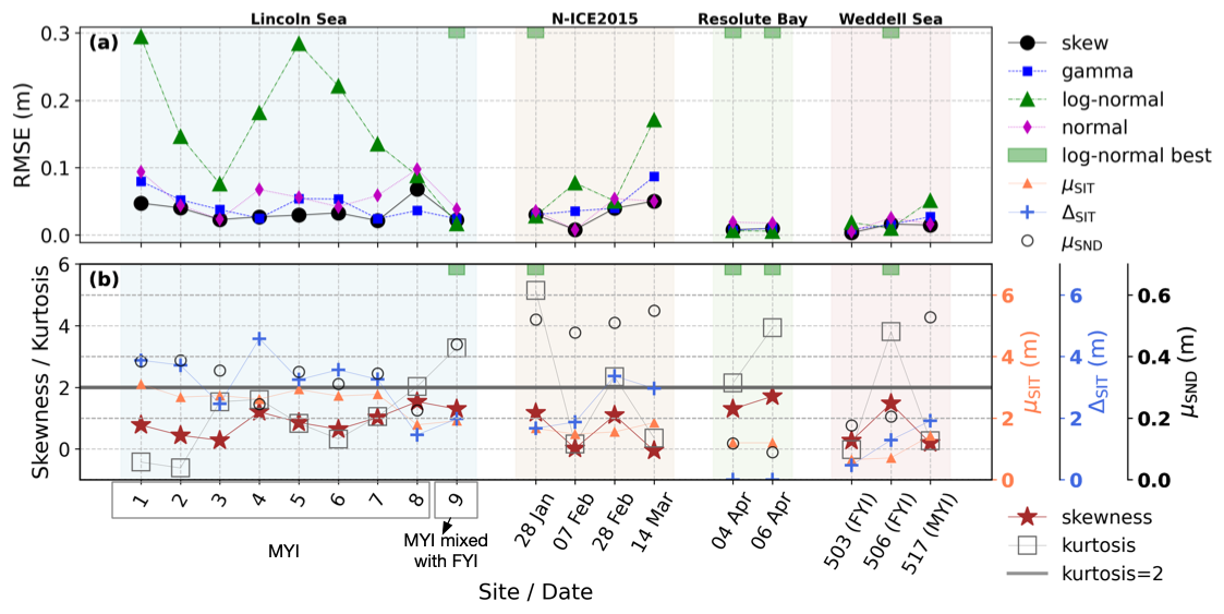
Figure 10 Time-series analyses of snow depth (SND) distribution over Lincoln Sea, N-ICE2015 (SYI), Resolute Bay (FYI), and Weddell Sea. Note that the thin lines connect samples within each test site for visual clarity only and do not imply time-series measurements. (a) Root-mean-square error (RMSE) between the fitted probability density functions (PDFs) and the measured SND values. The dates on which the log-normal performs best are marked by green bars. (b) shows skewness and kurtosis values calculated from the measured SND values. The mean SND (μ_SND), mean sea ice thickness (SIT, μ_SIT), and SIT range (${\mathrm{\Delta }}_{\mathrm{SIT}}=\mathrm{95}\mathit{\%}\mathrm{SIT}-\mathrm{5}\mathit{\%}\mathrm{SIT}$) of each transect are also plotted.

4.2.2 Regional comparison

The fitting performance at sites other than MOSAiC is shown in Fig. 10. For the Lincoln Sea where thick MYI dominates, the skew distribution provides the best fit of the observed SND from most transects. This result is consistent with observations from MOSAiC Nloop after 30 January 2020. Specifically, the skew distribution yields the lowest RMSE for transects 1–7, while for transects 4 and 7, both gamma and skew perform comparably. Transect 9 is located near the FYI zone and therefore contains a mixture of MYI and FYI (Haas et al., 2017). This transect exhibits kurtosis values greater than 2 in Fig. 10b, indicating an asymmetric and sharply peaked distribution. In this case, the log-normal distribution performs best, which is consistent with other FYI sites such as MOSAiC Runway and MOSAiC Sloop before 20 February 2020.

For N-ICE2015, the SYI was covered with a thick snow layer with μ_SND=0.50 m. However, μ_SIT is 1.58 m, similar to the Sloop transect but thinner than in the Lincoln Sea, MOSAiC Nloop, and MOSAiC Summer. Overall, as shown in Table 2, the skew distribution yields the highest accuracy with the smallest RMSE. This result is consistent with the SYI from MOSAiC Nloop after 30 January 2020 and the MYI from the Lincoln Sea. On 7 February and 14 March 2015, PDFs exhibit symmetric shapes, with skewness close to 0 in Fig. 10b. This explains why skew and normal distributions perform equally better, while log-normal does not provide a proper fit.

For Weddell Sea samples, MYI floe 517 exhibits μ_SIT of 1.43 m covered by a thick snow layer (μ_SND=0.53 m), where the snow and ice conditions are similar to those of the N-ICE2015 samples. The skew provides the best fit, consistent with the performance observed in the N-ICE2015 transects. FYI floes 503 and 506 have an average SIT of 0.69 m, which is the thinnest ice in the entire dataset. Floe 506 exhibits higher skewness than floe 503 and kurtosis >2, indicating an asymmetric and sharply peaked distribution (Fig. S4). In this case, the log-normal distribution performs best, consistent with the results of FYI from MOSAiC Runway and Resolute Bay. However, floe 503 shows poor performance for the log-normal distribution. This can be explained by the near-symmetric shape of the SND histogram, with a small skewness value of only 0.26, which diminishes the advantage of log-normal's ability to model asymmetry.

Resolute Bay (FYI) has snow and ice conditions similar to those at the MOSAiC Runway. The fitting results shown in Fig. 10 indicate that the log-normal distribution provides the highest accuracy, with the lowest RMSE values. This result is consistent with the FYI results from MOSAiC Runway samples.

4.2.3 Dependence on ice age and thickness

To analyse the dependence of the fitting performance on ice age and SIT, we categorize the RMSE values based on the μ_SIT interval using all samples from the non-summer datasets, shown in Fig. 11a. In general, for ice thinner than 1.5 m (mainly from FYI), log-normal provides the most accurate fit. For μ_SIT between 1.5–2 m, the samples are a mixture of ice ages, and both the gamma and the skew distributions perform well. When the ice exceeds 2 m (all from SYI and MYI), the skew provides the best fit. Note that the choice of thresholds at 1.5 and 2 m is based on the observed transition in the best-fitting distribution from the MOSAiC Sloop time-series observations. Specifically, SND fitting performance over FYI is shown in Fig. 11b–c, where RMSE exhibits a dependence on μ_SIT. Log-normal shows the best fitting performance for μ_SIT<1.5 m; however, its performance deteriorates significantly with increasing μ_SIT, while gamma and skew provide better fits. For SYI and MYI (Fig. 11d–g), the skew distribution always performs the best, and RMSE does not show dependence on μ_SIT. The MOSAiC Summer results, shown in Fig. 11h–i, indicate that for a very thin (μ_SND=0.07 m) and smooth snow layer, the log-normal provides the best fit and shows no dependence on μ_SIT.

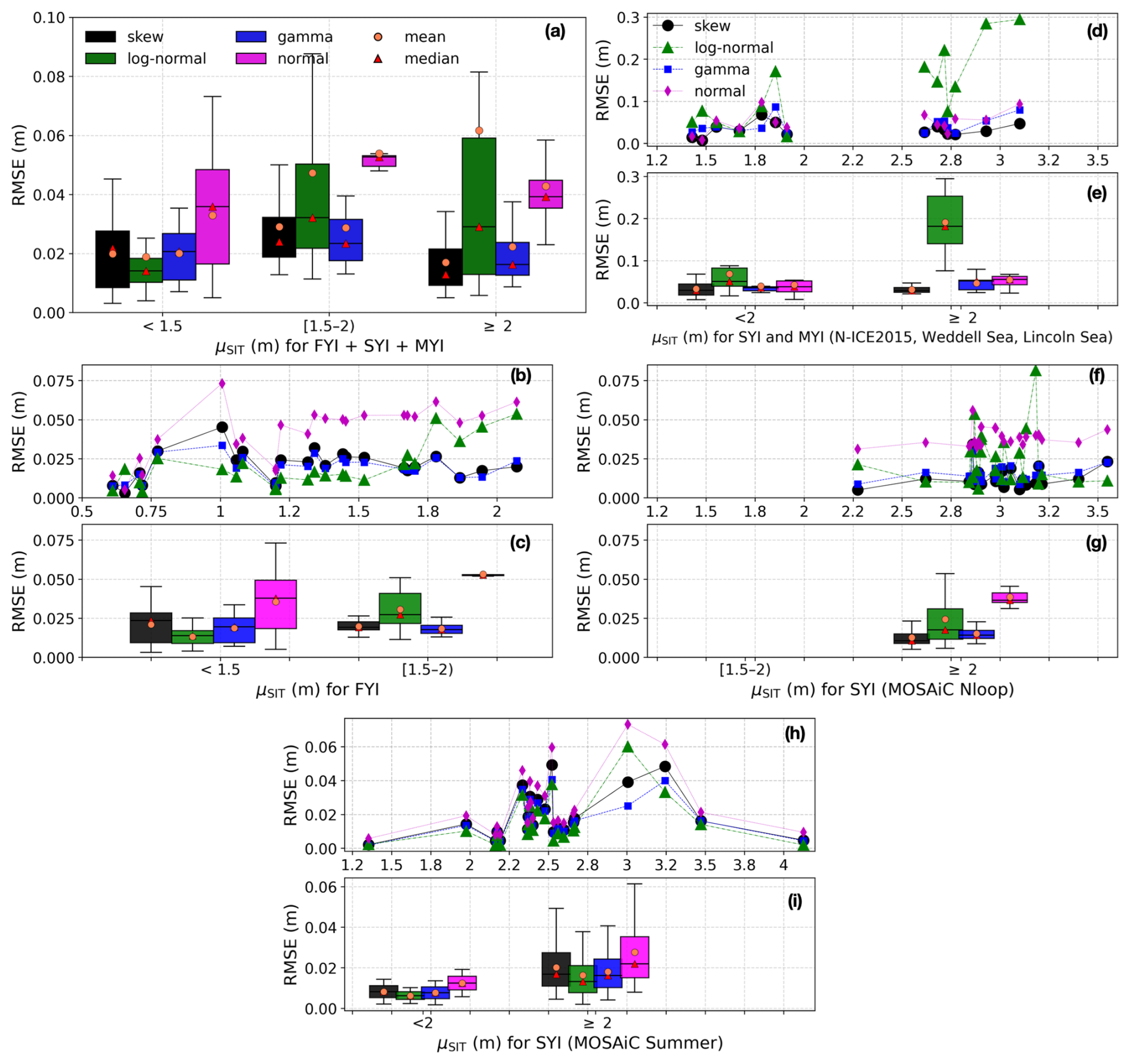
Figure 11 Boxplots of RMSE between the fitted probability density functions (PDFs) and the snow depth (SND) observations. μ_SIT denotes the mean sea ice thickness (SIT) of each transect. (a) All non-summer samples combined FYI, SYI, and MYI; the same samples are separated by ice types in panels (b)–(g). (h–i) Summer samples: MOSAiC Summer. Specifically, (b–c) FYI: MOSAiC Sloop, MOSAiC Runway, Weddell Sea, and Resolute Bay. (d–e) SYI and MYI: N-ICE2015, Weddell Sea, and Lincoln Sea. (f–g) SYI from MOSAiC Nloop. Note that SYI and MYI in panels (d) and (f) are shown separately for better visualization, as otherwise the points would be overcrowded. For each box, the top, middle, and bottom boundaries correspond to the third (Q3), median, and first (Q1) quartiles. The whiskers extend to the values within Q1 − 1.5× (Q3 − Q1) and Q3 + 1.5× (Q3 − Q1).

We interpret the differences in SND distributions between FYI and SYI/MYI primarily as a snow residence-time effect: snow remains on older ice for a longer period, allowing more time for accumulation and wind-driven redistribution, which progressively modifies the distribution. The snow with shorter residence time is typically well described by a log-normal distribution, evidenced by the snow over younger ice type in our observations at MOSAiC Runway, Resolute Bay, and the early stage of MOSAiC Sloop. In contrast, longer exposure to wind-driven redistribution progressively modifies the snowpack and can shift the SND distribution away from log-normal behaviour, as observed from the late stages of MOSAiC Sloop (after 20 February 2020), MOSAiC Nloop (after 30 January 2020), Lincoln Sea, N-ICE2015, Weddell Sea (MYI).

The apparent dependence of the SND distribution on the SIT for FYI can be attributed to the inherent positive relationship between the ice age and the SIT during the growth season, such that the SIT effectively serves as a proxy for the detailed ice age on a weekly scale. The observed SIT dependence therefore mainly reflects differences in ice age (and associated snow residence time), rather than thickness alone. Consequently, the threshold of 1.5 m should not be considered universal; it can vary with the regional ice growth rate and the occurrence and intensity of meteorological events that promote snow redistribution. It is also worth noting that although log-normal performs best for SND on younger and thinner ice, it can have a large deviation for thicker and older ice (μ_SIT>2 m, see Fig. 11a, e, and g). In contrast, the skew distribution is less prone to large deviations from the observed SND distributions. Therefore, the skew distribution can be a more robust choice for describing the SND distribution particularly over heterogeneous or unknown ice types, offering a balance between the accuracy and stability of the SND distribution fitting.

4.3 Correlation length of snow depth

The correlation length of SND for each transect at all test sites was estimated using the method in Sect. 3.2. Note that four transects, namely the MOSAiC Nloop transect on 27 February 2020, MOSAiC Summer transect on 27 June 2020, and Lincoln Sea transects 4 and 5, were excluded because their semi-variograms do not reach a constant semi-variance value, preventing accurate estimation of the sill and effective range (i.e. correlation length). This occurs because semi-variogram analysis can fail to detect slope-change points at large length scales due to undulations in the variogram introduced by local non-stationarities (Moon et al., 2019). In such cases, the effective range cannot be robustly estimated from the semi-variogram, and more advanced approaches such as multifractal temporally weighted detrended fluctuation analysis are required (Moon et al., 2019).

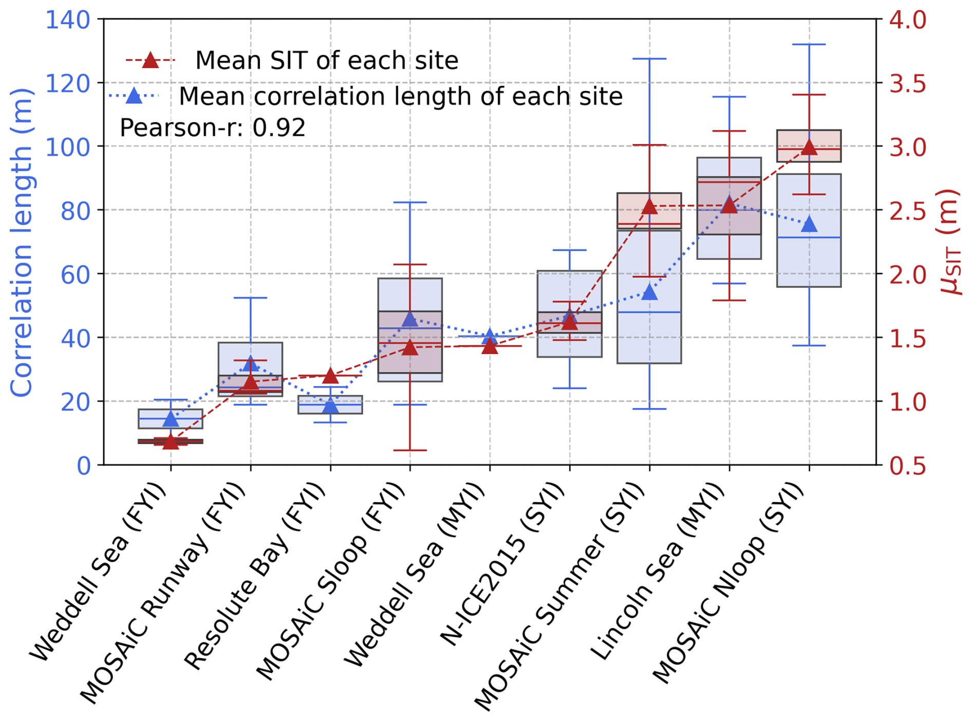
Figure 12 The relationship between snow depth (SND) correlation length and sea ice thickness (SIT). μ_SIT denote the mean SIT over each transect. For each box, the top, middle, and bottom boundaries correspond to the third (Q3), median, and first (Q1) quartiles. The whiskers extend to the values within Q1 − 1.5 × (Q3 − Q1) and Q3 + 1.5 × (Q3 − Q1). The red dash and blue dot lines indicate the mean SIT and mean correlation length for each site, with a correlation of Pearson-r=0.92.

The correlation lengths of the transects within each site are shown in Fig. 12. We observe that thicker ice is associated with a larger mean correlation length. The mean correlation length and mean SIT of each site are plotted as blue and red lines, respectively, showing a high correlation of 0.92. In general, the mean correlation length for FYI is 39±25 m (mean ± standard deviation). For smooth and thin snow-covered SYI in summer (MOSAiC Summer), it increases to 54±28 m, while snow-covered SYI and MYI in the non-summer season (i.e. excluding MOSAiC Summer) exhibit the longest correlation length, averaging 72±25 m.

For FYI, the correlation lengths vary between 10–80 m, as shown in Fig. 12. The range is consistent with observations from undeformed FYI where the 10 m length scale is associated with wind-driven dune formation (Moon et al., 2019). On larger scales (30–100 m), the governing processes may involve interactions between individual dunes, such as their gradual movement, merging, or dispersal over time. Specifically, for the three sites (Weddell Sea, MOSAiC Runway, and Resolute Bay) covered by thin ice with μ_SIT<1.2 m, the mean correlation length is approximately 14±8 and 19±8 m for FYI in the Weddell Sea and Resolute Bay, respectively. For MOSAiC Runway (FYI), the mean correlation length is 32±18 m. For MOSAiC Sloop, where FYI is growing with μ_SIT of 1.4 m, the mean correlation length is 46±26 m, with greater variability than other FYI possibly due to the broader range of SIT.

For SYI and MYI, the SIT values for the Weddell Sea and N-ICE2015 are ∼1.5 m, similar to the MOSAiC Sloop. The mean correlation lengths are approximately 45±17 m, consistent with those observed for MOSAiC Sloop. Sturm et al. (1998) reported that snow-surface correlation lengths vary from 3 to 70 m, averaging 13–23 m, based on observations from FYI and MYI in the Bellingshausen, Amundsen, and Ross Seas. In this study, the correlation lengths derived from two FYI floes and one MYI floe from the Weddell Sea are 8, 20, and 40 m, respectively, with a mean value of 23 m, which agrees well with the observations from Sturm et al. (1998).

For SYI and MYI thicker than 2 m, including MOSAiC Summer, Lincoln Sea, and MOSAiC Nloop, the correlation length shows larger mean values and greater variation compared to others. The mean correlation lengths are 75±24 m for the MOSAiC Nloop and 82±21 m for the Lincoln Sea. For MOSAiC Summer, the mean correlation length is 54±28 m, less than that of the Lincoln Sea, despite a similar mean SIT. This can result from the very thin snow layer (μ_SND=0.07 m) during the melting season, where the surface was smooth and therefore exhibits reduced spatial correlation.

The positive correlation between correlation length and SIT can be explained by the physical processes that shape the snow surface features. Small correlation lengths are likely associated with the spatial scale of individual snow dunes (Filhol and Sturm, 2015), beyond which SND at one location provides little information about that at another. In contrast, on rougher MYI, larger correlation lengths are expected, as prominent surface features, such as hummocks and ridges, affect snow accumulation over broader spatial scales. The surface topography of FYI (MOSAiC Sloop) and SYI (MOSAiC Nloop) captured by ALS is provided in Fig. S5, visualizing that SYI exhibits more pronounced surface features than FYI, which likely results in larger correlation lengths.

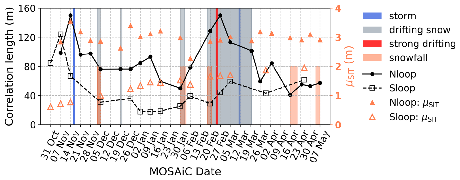
Figure 13 Time-series analysis of correlation lengths from MOSAiC northern loop (Nloop) and southern loop (Sloop). The relevant climate events such as storm, snowfall, and drifting snow are from Wagner et al. (2022).

To investigate the temporal changes of the spatial heterogeneity of snow cover, we analyse time-series variograms from the MOSAiC Nloop and Sloop sites. For MOSAiC Nloop, we observed a consistent increase in correlation length between 30 January and 27 February 2020, following snowfall and drifting-snow events that began on 30 January and 18 February 2020 (Fig. 13). A major drifting snow event occurred on 24–25 February 2020, coinciding with the largest correlation length observed on 27 February 2020, indicating a snow correlation length exceeding 150 m. Slight increases in snow correlation length were also observed on 26 December 2019, 24 April 2020, and 7 May 2020, coinciding with snowfall or drifting snow events. One possible process is that, during significant snowfall or drifting snow events, the valleys between the snow dunes become filled (Iacozza and Barber, 2010), leading to larger and more continuous snow structures, represented by increasing correlation lengths. This infill alters the pattern of the SND distribution and influences subsequent snow redistribution processes. For MOSAiC Sloop, although the changes in snow correlation length are less pronounced than those at MOSAiC Nloop, there is a steady increase from around 28 to 60 m during the drifting snow event from 20 February to 20 March 2020. These results suggest that drifting snow events have a greater impact on increasing snow correlation length over rougher ice (MOSAiC Nloop) compared to smoother ice (MOSAiC Sloop).

5 Discussion

5.1 Comparison with previous studies

Mallett et al. (2022) evaluated the skew distribution using SND transects spanning FYI to MYI. This study extends previous analyses by further investigating the effects of SIT and meteorological events on SND distribution. Mallett et al. (2022) showed that the skew distribution provides the best fit for SND over MYI, which is consistent with our results (Fig. 11e and g), with two exceptions. First, during summer, when the snow cover is very thin (mean 7 cm) over SYI (Fig. 11h and i), the log-normal distribution performs best. Second, during the early stage of snow accumulation over the MOSAiC Nloop (Fig. 8a), prior to wind-driven redistribution, the log-normal again provides the best fit. These two exceptions complement the findings of Mallett et al. (2022) and demonstrate that meteorological events and seasonality are essential in regulating SND distribution. Note that in these two cases, the improvement in the log-normal over skew distribution is modest (≈20 %–25 %), calculated from Table 2 using $({\mathrm{RMSE}}_{\mathrm{skew}}-{\mathrm{RMSE}}_{\text{log-normal}})/{\mathrm{RMSE}}_{\mathrm{skew}}$. However, the skew significantly outperforms the log-normal by ≈60 %–80 % in other SYI and MYI cases. In particular, large RMSE values of log-normal are observed for MOSAiC Nloop after 30 January 2020 in Fig. 8a and the Lincoln Sea and N-ICE2015 in Fig. 10. Hence, although the log-normal distribution performs best in these two exceptions, the skew distribution exhibits greater stability and is less sensitive to extreme deviations from the observed SND distributions. For practical applications, the skew distribution therefore provides a more robust representation of SND distribution over regions containing mixed ice types or lacking a priori knowledge of ice type.

Mallett et al. (2022) quantified the CV of the snow in MYI. We extend the analysis to include FYI and obtained an overall CV of 0.50. The value reported by Mallett et al. (2022) (CV = 0.42) falls within the 95 % prediction interval of our empirical fit (Fig. 7b), indicating consistency across the datasets. Additionally, we demonstrate that CV shows no dependence on SIT, suggesting that the linear relation (Eq. 7) to estimate sub-grid or footprint-scale SND variability from mean SND can be applied across a range of SIT conditions. We also observe that flooding can reduce CV, revealing that flooding can imprint a measurable signature on the SND distribution.

Wever et al. (2021a) used GEM on the floe-scale (400 m × 400 m) and GEM inside the terrestrial laser scanning (TLS) field (80 m × 80 m) to characterise spatial variability in SND and SIT. This study uses GEM floe-scale data because the 400 m × 400 m coverage can represent an individual floe and is consistent with the spatial scale across other test sites. Wever et al. (2021a) reported SND and total thickness (snow + ice) for each floe (503, 506, and 517) using both datasets. The violin plots (Figs. 3 and S3) summarize SND and SIT for FYI (503 and 506) and MYI (517) which are consistent with Wever et al. (2021a). Beyond this, we further explored the PDF that best fits the SND distributions related to ice age and SIT (Figs. 10–11).

Using MOSAiC time-series data, this study analysed the weekly evolution of SND statistics, providing new insights for the snow community. Liston et al. (2020) reported a strong correlation between mean SND and ice age (in days), suggesting that it is not sufficient to know only whether the ice is FYI; we must also know the age of FYI (in days or weeks). We examine how the best-fitting statistical distribution of SND evolves using weekly MOSAiC measurements (Fig. 8). For the Sloop (FYI) during the growing season, we observe a clear shift in the SND distribution from log-normal to gamma/skew as SIT continues to increase. These results not only reinforce the hypothesis that ice age strongly controls snow evolution (Liston et al., 2020), but also provide new quantitative insights into the temporal variability of snow layers. Furthermore, Moon et al. (2019) indicated that topography and wind redistribution are two main factors controlling the spatial variability of SND and its correlation length. Our results support the role of wind redistribution: drifting snow events increase correlation length (Fig. 13), consistent with the growth of snow-dune size (Iacozza and Barber, 2010; Moon et al., 2019). We also examine the influence of surface topography on SND distributions using ALS data for MOSAiC Nloop and Sloop (Fig. S5). However, no pronounced snow-topographic features were observed from December 2019 to February 2020, spanning the period before and after the transition in the best-fitting PDFs. Previous studies suggest a dependence of the correlation length on ice types (Fetterer and Untersteiner, 1998; Iacozza and Barber, 1999). The findings of this study are consistent with this dependence on ice types and further suggest a clear relationship between correlation length and SIT (Fig. 12).

5.2 Links to sea ice models

Sea ice models within coupled climate models are key tools for quantifying high-latitude climate variability and supporting seasonal sea ice prediction (Holland et al., 2010; Hamilton and Stroeve, 2016). Because even 1 km configurations cannot explicitly resolve the strong sub-grid heterogeneity of SIT and associated processes, most models represent thickness variability using an ice thickness distribution (ITD) framework (Thorndike et al., 1975). In practice, the ITD is discretized into a finite number of thickness categories. A proper selection of the number of categories is essential to ensure a meaningful simulation of key sea ice variables, such as the ice volume (Bitz et al., 2001; Lipscomb, 2001; Hunke, 2014; Massonnet et al., 2019). In addition to the ITD, snow parameterizations are a key source of uncertainty and control in sea ice models. Liston et al. (2018, 2020) showed that spatial variability in SND strongly modulates conductive heat flux, winter ice growth, and the timing and magnitude of surface melt, through its control on insulation, surface temperature, and radiative processes. Castro-Morales et al. (2014) evaluated two snow representations: one in which the SND is independent of the underlying SIT, and another in which the snow is distributed proportionally to the ITD. Their results indicate that the latter approach improves the simulation of thermodynamic ice growth during the ice-formation period. Castro-Morales et al. (2014) therefore emphasized the need for large-scale field observations to establish representative and robust statistical relationships between snow and sea ice. Our results provide new quantitative insights into this perspective. Specifically, Fig. 11 demonstrates that SND distributions exhibit a clear dependence on SIT for FYI, which can be used to evaluate and refine category-specific snow parameterizations in models. Moreover, our findings on SND distributions across ice ages and SIT values can be incorporated into ITD frameworks to better represent the statistical coupling between snow and ice, thereby improving simulations of thermodynamic ice growth during the ice-formation period. As a simplified alternative, a skew distribution can serve as a robust candidate when assuming a single universal distribution for the snow field across the ITD categories.

5.3 Links to satellite observations

To derive SIT from satellite altimetry, freeboard measurements must be combined with SND information. However, the horizontal resolution of snow depth products (25–100 km) is much coarser than that of along-track freeboard measurements (15 m–2 km) (Glissenaar et al., 2021), creating a scale mismatch that necessitates parameterized representations of sub-grid snow redistribution within altimeter footprints. Previous approaches have introduced empirical redistribution functions based primarily on freeboard (Kwok and Cunningham, 2008; Petty et al., 2020), with coefficients derived from airborne observations during Operation IceBridge (Petty et al., 2020). The findings of this article highlight that ice age, in addition to freeboard, can be a potentially important factor to consider in the empirical snow-redistribution functions for laser-altimetry-based SIT retrieval.

Because SIT retrieval from altimetry depends explicitly on SND through hydrostatic equilibrium, SND variability within the footprint directly propagates into SIT retrieval uncertainty. Given a large-scale mean SND, the standard deviation of SND can be inferred using the CV (Fig. 7). The statistical distribution of SND derived in this study provides a more comprehensive representation of sub-grid SND variability. Specifically, the most appropriate distribution (e.g. log-normal or skew) can be selected according to the ice age and SIT. For a log-normal distribution, which is defined by two parameters, the mean and standard deviation are sufficient to determine the distribution parameters and reconstruct the fitted PDF. The skew distribution requires three parameters, namely mean, standard deviation, and the skewness (as given in this study). Once the PDF is fitted, additional SND statistics, including modal values and percentiles, can be derived. From a satellite perspective, the modal SND is particularly relevant because it is the most frequently occurring SND within a satellite footprint and can be associated with the dominant surface condition. These statistics provide a more complete characterization of sub-grid snow variability and can be propagated to quantify uncertainty in SIT retrieval at sub-kilometre scale.

5.4 Limitations

A limitation of this study is the regional datasets. The analysis in this article is based on the selected test sites rather than on unified pan-Arctic and -Antarctic datasets. Nevertheless, the sites were carefully chosen to span various snow and ice types and each contains thousands of samples, ensuring statistically robust analysis. However, SND distributions can be sensitive to many local factors such as ice topography, snowfall, wind redistribution, flooding, and melt processes. Consequently, extending these findings to the hemispheric scale requires thorough evaluation using large and comprehensive datasets. Despite this limitation, the regional cases analysed here, supported by high-quality in-situ measurements, provide new insights into how SND distributions depend on ice types and thicknesses at the sub-kilometre scale. To assess the regional representativeness of the findings of this study, we summarize the dominant climatic and ice-type characteristics captured at each test site in the following.

The MOSAiC Nloop and Lincoln Sea datasets represent the thick (μ_SIT>2.5 m) and deformed SYI and MYI conditions. The consistent PDF-fitting performance between Nloop and the Lincoln Sea supports the conclusion that the SND distribution depends on ice age. Therefore, these results are most applicable to thick and deformed SYI and MYI types. The N-ICE2015 dataset, combined with observations from the Weddell Sea (MYI) during austral winter, represents conditions of substantial snow loading (μ_SND>0.5 m) and susceptibility to flooding. These sites are particularly relevant for characterizing SND distributions under heavy snow accumulation and snow–ice formation processes. The MOSAiC Sloop reflects a growing FYI evolving from newly-formed ice to fully developed FYI, with SIT increasing from <1 to ∼2 m between October and May. These observations are most representative of the evolution of snow over growing FYI, from initial formation through full development to the pre-melt season. The MOSAiC Runway and Resolute Bay datasets represent relatively level FYI with thin and smooth snow cover. Among all sites, they exhibit the lowest mean SND and standard deviation and are therefore most representative of newly-formed snow over young ice. The MOSAiC Summer represents SYI that persists into summer with a shallow snow layer (∼7 cm). This case demonstrates that, despite the same ice type (SYI), SND distributions can differ substantially between winter and summer. These observations are most applicable to thin snow-covered SYI during the melt season.

Another limitation concerns the measurement accuracy of SND and SIT obtained from the magnaprobe and EM instruments. The magnaprobe has a precision of 3 mm. Given that the typical mean SND within each transect is several to tens of centimetres, 3 mm is small relative to the SND measurements. In the analyses, we use μ_SND computed from all samples along each transect rather than an individual sample, which further reduces the influence of measurement uncertainty. Each transect contains hundreds of samples, ensuring that the inferred PDFs are statistically robust; therefore measurement error from a single sample has a negligible effect on the overall distribution shape. When evaluating the fitting performance, the differences in RMSE between two PDFs less than 3 mm are considered comparable (Table 2), consistent with the instrumental precision of the magnaprobe. The precision of the EM measurements is approximately 0.1 m on level ice. Similarly, we use μ_SIT calculated by averaging all samples along each transect, rather than individual measurements, thus reducing the influence of measurement uncertainty on the reported SIT-dependent relationship. The μ_SIT is used primarily for mean-SIT binning, so the influence of measurement uncertainty on the results is expected to be limited.

5.5 Recommendations for practical applications

This study examines the influence of ice age, SIT, and meteorological conditions on the most appropriate PDF to describe SND observations. In the context of practical applications, we recommend the following considerations for characterizing sub-kilometre SND distributions:

1. The ice age should be explicitly considered. Ice age represents the effective snow residence time on a given ice floe and therefore controls the degree of snow accumulation and wind redistribution. SND distributions vary with ice age: newly accumulated snow on younger ice (often FYI) is typically well described by a log-normal distribution, whereas progressive wind redistribution, compaction, and drift processes reshape the distribution toward a skew shape. Consequently, snow over older and thicker ice (often SYI and MYI), where the snow has a longer residence time, is generally better characterised by a skew distribution.

2. During the growth season, thicker ice generally corresponds to older FYI. Hence SIT acts as a proxy for fine-scale ice age (e.g., in days or weeks) across the evolution from newly formed to fully developed FYI. The apparent SIT dependence of PDF performance therefore mainly reflects relations to snow residence time. Accordingly, different PDFs are recommended for FYI at different growth stages. For thinner FYI (μ_SIT<1.5 m), the log-normal distribution is generally appropriate, whereas for thicker FYI (μ_SIT>1.5 m), the skew and gamma distributions provide the best performance. The 1.5 m threshold should not be regarded universal, as it depends on the rate of ice growth and the timing and intensity of redistribution events, which may vary regionally and seasonally.

3. Meteorological redistribution events should be explicitly considered. Wind-driven redistribution can induce temporal transitions in SND distributions, even within the same ice type, shifting behaviour from log-normal to skew distribution. During the melting season, when the snow layer is thin and smooth, the log-normal distribution performs best.

4. Although the log-normal distribution performs best for snow with a short residence time, its performance can deteriorate substantially over older and thicker ice. The skew distribution demonstrates greater robustness across types, offering a balance between fitting accuracy and stability, and is therefore suitable for applications spanning heterogeneous ice conditions or lacking a priori knowledge of ice types.

6 Conclusions

This study provided a systematic assessment of sub-kilometre SND distributions across diverse ice types and seasonal conditions. Based on field observations that covered FYI, SYI, MYI, flooded ice, and melt-season conditions, the results demonstrated that SND statistics are influenced by ice ages, SIT, and meteorological events.

During the growth season, the SND over FYI increases linearly with the SIT, reflecting the concurrent formation of ice and snow. Despite differences in ice types, CV remains approximately constant (≈0.50), indicating that sub-grid variability can be inferred from mean SND. Flooded ice exhibited reduced variability relative to non-flooded sites, suggesting that flooding can imprint a measurable signature in the SND distribution. Moreover, the PDF that best describes the SND distribution is governed by ice age, which represents the effective residence time of snow on a given ice floe and thus controls its accumulation and redistribution. New snow on young and thin FYI is best represented by a log-normal distribution, whereas redistributed snow on older and thicker ice is best represented by a skew distribution. In the MOSAiC Nloop and Sloop observations, this transition occurred after approximately three to four months of snow residence time. The threshold of approximately three to four months used to distinguish “new” from “redistributed” snow can be subjective to ice type, regional conditions, and seasonal forcing. Therefore, further validation will be required using large-scale time-series observations in the future. During the FYI growth season, the dependence of fitting performance on SIT reflects the role of SIT as a proxy for fine-scale ice age (e.g. in days or weeks). Meteorological events can induce temporal transitions in distribution shape within the same ice type, underscoring the dynamic coupling between wind redistribution and ice conditions. Although the log-normal distribution performs well under specific conditions (e.g. new or melt-season snow), its performance deteriorates significantly over older ice (e.g. SYI and MYI). The skew distribution provides a good compromise between robustness and accuracy and is therefore recommended for scenarios involving heterogeneous ice types. Semi-variogram analysis revealed that the correlation length of SND increases with SIT, indicating an association between SIT and the spatial variability of SND. Snowfall and strong drifting snow events further enhance correlation length by smoothing small-scale variability and strengthening larger snow structures.

All these findings identify snow residence time and ice type as key controls on sub-kilometre SND variability. By clarifying how SND distributions change with ice ages, thicknesses, and redistribution processes, this study improves our understanding of how snow evolves on different types of sea ice under various meteorological conditions. The results provide practical recommendations for representing snow variability and SND distribution at sub-kilometre scale, with potential applications in climate modelling and in improving uncertainty estimates for remote-sensing-based SIT retrievals. Future work involves characterising the regional and temporal variation in SND by integrating high-resolution surface topographic measurements (e.g. terrestrial laser scanner) of snow bedforms.