Analysis of long-term dynamic changes of subglacial lakes in the Recovery Ice Stream, Antarctica

The dynamic activity of subglacial lakes plays a crucial role in modulating glacial processes and the mass balance of the Antarctic ice sheet. The Recovery Ice Stream (RIS), projected to experience significant mass loss in East Antarctica during coming centuries, requires continued investigation of its subglacial dynamics. In this study, we re-examine and update the outlines of nine active subglacial lakes identified before 2012 and identify 14 additional new active lakes (RecN1-RecN14) using ICESat-2 data. By synthesizing multi-source altimetry data (ICESat, IceBridge, ICESat-2), we establish a 21-year (2003–2023) elevation change time series for lakes in the RIS. This extended observational record reveals that the drainage regime in RIS is characterized by long-term, sustained water transport. Through crossover analysis, we precisely identify elevation changes and elucidate internal spatiotemporal patterns across distinct lake sectors, revealing significant disparities between lake centers and their peripheries. We demonstrate that the original lake Rec1 comprises two distinct lakes and analyze their hydrological connection, supporting the previously proposed hypothesis of two subglacial drainage outflows in the RIS. Furthermore, quantitative volume change analysis along the constructed subglacial hydrological networks reveals clustered filling-draining patterns. Specifically, we identify for the first time a cascading drainage event involving ten lakes and spanning over approximately 1000 km, revealing a highly connected subglacial hydrological system in this region. This study advances the understanding of subglacial lake hydrological dynamics in the RIS, thereby informing the evolution of the Antarctic subglacial system.

1 Introduction

Active subglacial lakes in Antarctica play critical roles in modulating ice stream velocities and outlet glacier dynamics (Stearns et al., 2008; Siegfried et al., 2016), influencing subglacial hydrology (Siegert et al., 2016; Napoleoni et al., 2020), and serving as a crucial component in understanding the mass balance of the Antarctic ice sheet (Livingstone et al., 2022). According to the most recent comprehensive inventory of subglacial lakes, there are about 140 active subglacial lakes in Antarctica (Livingstone et al., 2022). The Recovery Ice Stream (RIS) is located in East Antarctica, and thus far, a significant number of active subglacial lakes have been discovered in this region (Smith et al., 2009; Fricker et al., 2014). It is predicted that RIS will become one of the areas with severe mass loss in East Antarctica in the coming centuries, bearing consequential implications for the mass balance of the East Antarctic ice sheet and global sea level rise (Golledge et al., 2017). Therefore, long-term monitoring of the dynamic changes of subglacial lakes in the RIS is essential for understanding the subglacial hydrological processes in this region and predicting potential changes in the RIS in the future (Dow et al., 2018).

The filling-draining events of active subglacial lakes are typically associated with fluctuations in surface elevation, leading to increases and decreases in surface elevation. Therefore, satellite altimetry offers a distinct advantage by providing extensive coverage and long-term data on ice surface elevations (Fricker et al., 2016), opening new avenues for identifying active subglacial lakes and monitoring their activity (Fricker et al., 2007; Fricker and Scambos, 2009). Three primary methods are employed to detect surface elevation changes using satellite altimetry data. The first is the repeat-track analysis method, which involves resampling the repeated measurement tracks from different times to a reference track, allowing for the calculation of elevation changes at the same location relative to the initial measurement time (Smith et al., 2009). This approach is commonly applied to laser satellite altimetry data, such as ICESat and ICESat-2, due to their strictly repeatable ground tracks. The second is the crossover analysis method. This approach involves obtaining the elevation data at the crossovers where the ascending and descending tracks intersect, and then differencing the elevation data to obtain the changes at the same location over different time periods (Fricker et al., 2010; Leong, 2021). This crossover analysis method can be applied to both laser altimetry data, such as ICESat (Shi et al., 2009), and ICESat-2 (Leong, 2021), as well as radar altimetry data, such as Envisat (Fricker et al., 2010). The third is the digital elevation model (DEM) differencing method. This method involves establishing a reference DEM or incorporating an external DEM, and then comparing it with satellite altimetry data collected at different times to calculate the surface elevation changes over a specific time interval (Siegfried and Fricker, 2021; Fan et al., 2023). In recent years, the commonly used radar altimetry satellite CryoSat-2 employs SARIn mode to monitor active subglacial lakes. In this mode, the distribution of data points is relatively sparse, rendering both repeat-track analysis and crossover analysis less applicable. In response to this situation, the DEM differencing method is often adopted. This approach involves accumulating sufficient altimetry data over a specific period to generate a DEM, which is then compared to the reference DEM (Kim et al., 2016), thus obtaining surface elevation changes over a specific time interval and facilitating the monitoring of elevation changes in subglacial lakes.

In the RIS region, the first four subglacial lakes (referred to here as Lakes A–D) were identified using a combination of ice surface elevation changes from ICESat and satellite imagery (Bell et al., 2007). These lakes are located in extensive, flat, and featureless ice surface areas, delineated by upstream troughs and downstream ridges. In subsequent studies, Langley et al. (2011) and Diez et al. (2019) examined the subglacial environments of these lakes and found that only the southern part of Lake A had a typical subglacial lake area, while the other areas had drained and had wet beds. Downstream from Lakes A–D, Smith et al. (2009) identified 11 active subglacial lakes based on surface elevation changes from repeat-track analysis using ICESat data between 2004 and 2008. This study also offered initial evidence of hydrological connectivity within the RIS (Smith et al., 2009). By combining ICESat satellite altimetry data and IceBridge airborne altimetry data, using an improved repeat-track analysis that divides tracks into narrower strips for closer repetition to reduce cross-track slope errors compared to Smith et al. (2009), the active subglacial lakes in RIS were re-investigated, and the existence of nine subglacial lakes (Rec1-Rec9) between 2003 and 2012 was ultimately confirmed (Fricker et al., 2014).

Previous studies utilized satellite altimetry data to monitor subglacial lake activity in the RIS region until 2012. According to simulations based on the Glacier Drainage System model (GlaDS), the basal hydrological system of the RIS has maintained an active state and is expected to continue this activity in the long term (Dow et al., 2018). Following the retirement of ICESat, a significant gap in continuous monitoring has limited our understanding of recent changes. The CryoSat-2 radar satellite provides only partial coverage through its SARIn mode, limited to lakes Rec1 and Rec2. During this monitoring gap, the Operation IceBridge airborne mission offers a valuable alternative, providing not only comprehensive coverage for lakes Rec1 through Rec6 but also extensive repeat survey data for the RIS over multiple years (Fricker et al., 2014). These features make IceBridge a significantly better choice for studying this area compared to CryoSat-2. Furthermore, the successful launch of ICESat-2 provides high-resolution and high-accuracy altimetry data of the Earth's surface, offering valuable opportunities for detailed investigation of the recent dynamics of subglacial lakes in the RIS region.

In this paper, the recently active subglacial lakes in the RIS region are investigated by using new satellite altimetry data from ICESat-2. The outlines of subglacial lakes in the inventory are updated, and several new subglacial lakes are also identified. Additionally, by integrating altimetry data from ICESat, IceBridge, and ICESat-2, the time series of elevation changes in subglacial lakes within the RIS region from 2003 to 2023 is obtained. Additionally, through crossover analysis, the variations in elevation changes at different locations within the lakes are investigated. Finally, the hydrological connections among subglacial lakes in the RIS are identified based on the subglacial hydrological networks and volume changes of the subglacial lakes.

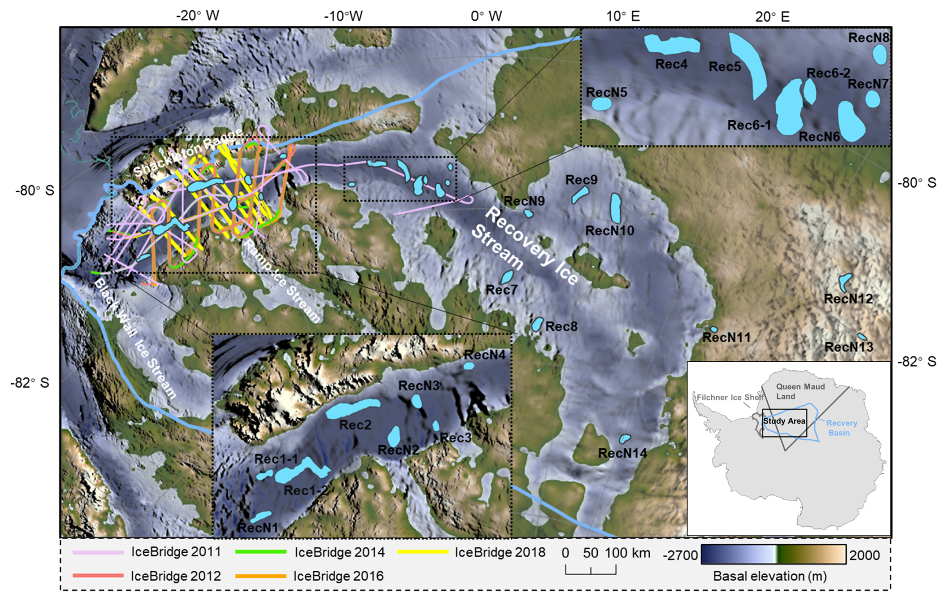
Figure 1 The inset map indicates the location of the study area. The main panel presents the bed elevation from BedMachine V3 (Morlighem, 2022), overlaid with the MODIS Mosaic of Antarctica (MOA) (Haran et al., 2014). The figure also highlights the flight lines from IceBridge campaigns in 2011, 2012, 2014, 2016, and 2018, as well as the locations of subglacial lakes. Two zoomed-in panels provide enlarged views of the lower and upper troughs of the RIS.

2 Study area and data

2.1 Study area

The Recovery Basin is situated in Queen Maud Land, East Antarctica, covering approximately 996 000 km², which represents about 8 % of the East Antarctic ice sheet's area (Rignot et al., 2008). As shown in Fig. 1, RIS is the core ice stream of Recovery Basin, contributing 58 % of the total flux to the Filchner Ice Shelf (Joughin and Bamber, 2005), extending into the interior of Recovery Basin with a distinctive funnel-shaped structure – narrower in the downstream area while widening in the upstream region (Jezek, 1999). RIS borders the Shackleton Range to the north, while to the south it develops two important tributaries, namely Ramp Ice Stream and the less active Blackwall Ice Stream (Eis, 2019). The RIS features a distinctive narrow bedrock trough that extends approximately 1000 km, reaching depths of 1500–2000 m below sea level (Fricker et al., 2014). The bedrock trough is divided into upper and lower sections by a ridge located at −17° W (Fricker et al., 2014). Most reported active lakes in the RIS region are located within the bedrock trough. The surface ice flow velocity increases from the upper trough to the lower trough, with speeds reaching approximately 870 m yr⁻¹ in the rapid ice flow region of the RIS (Floricioiu et al., 2014).

2.2 Data

2.2.1 Altimetry data

In this study, three altimetry missions, including ICESat satellite altimetry data from 2003–2009, IceBridge airborne altimetry data from 2011–2018, and ICESat-2 satellite altimetry data from 2018–2023, are combined to obtain the long-term dynamics of the subglacial lakes in the RIS. The detailed information of these altimetry data is illustrated in Table 1.

Table 1 The acquisition time of the altimetry data used in this study.

ICESat uses a single-beam laser altimeter equipped with a Geoscience Laser Altimetry System (GLAS) to sample the Earth's surface. The ground footprint of each laser pulse of ICESat is about 50–100 m in diameter, and the resolution along the satellite ground orbit is about 170 m (Abshire et al., 2005). Three identical lasers (Laser 1–Laser 3) were mounted on GLAS to ensure redundancy and extend the mission's operational lifetime. Laser 1 onboard ICESat malfunctioned 56 d after launch, resulting in very limited data collection. Additionally, the integration of its data with subsequent data requires various error corrections. Therefore, this study only utilizes data collected by Laser 2 and Laser 3. Laser 2 was shut down after the Laser 2c campaign, and was restarted following the failure of Laser 3, so the Laser 2d-Laser 2f campaign period occurred after Laser 3k (Borsa et al., 2014, 2019). The GLAH12 polar ice sheet elevation product provided by the National Snow and Ice Data Center (NSIDC) is adopted in this study. This product has been processed with a series of corrections including saturation correction, receiver gain filtering, data processing flags, ellipsoid correction, task period deviation correction (Sun et al., 2017).

Operation IceBridge is a large-scale polar aerial survey mission designed to bridge the data gap between ICESat and ICESat-2 satellites, hence the name “ice bridge” (Fricker et al., 2014). In the polar area, over 1000 aircraft survey flights have been conducted from 2010 to 2018. However, only five years of ice bridge operation tasks in 2011, 2012, 2014, 2016, and 2018 collected data on active subglacial lakes in the RIS. This study incorporates the Airborne Topographic Mapper (ATM) data from the IceBridge operation. To minimize uncertainty, we only retained data collected along the nadir track, which provides more precise ice surface elevation measurements and minimizes the influence of terrain undulations and tilt angles on the measurement results. The locations of flight lines used in this study from the IceBridge mission are shown in Fig. 1.

ICESat-2 is equipped with an Advanced Topographic Laser Altimetry System (ATLAS), which achieves centimeter-level accuracy in surface elevation measurements. ICESat-2 Land-Ice Surface Heights product ATL06 and the Slope-Corrected Land Ice Height Time Series product ATL11 are employed to analyze elevation changes in subglacial lakes within the RIS region. The ATL06 data, oriented along the orbital path, utilize 40 m track segments to calculate average heights, with an along-track resolution of 20 m (Smith et al., 2019). The time span of the ICESat-2 ATL06 data used in this study extends from October 2018 to June 2023 (Cycle 1 to Cycle 19, as shown in Table 1). ATL11 provides a temporally organized land-ice surface height time series derived from the ATL06 product (Smith et al., 2023b). Height variations in the ATL11 data are computed for successive observations (spaced 91 d apart) along individual ICESat-2 ground tracks in polar regions, with an along-track resolution of 60 m. Due to suboptimal overlap of repeated orbits during the initial two cycles, ATL11 began providing products from cycle 3 onward, starting after 29 March 2019. Additionally, ATL11 offers elevation data at crossovers with a temporal resolution reduced from the original 91 d cycle to one month or even a few days.

2.2.2 Ice thickness and bedrock elevation data

The ice thickness data provided by the latest Antarctic terrain dataset BedMachine V3 (Morlighem, 2022) are used. The ice thickness data with 500 m horizontal resolution are sourced from airborne ice-penetrating radar surveys (Morlighem, 2022). The surface elevation is derived from the surface DEM of Reference Elevation Model of Antarctica (REMA) (Howat et al., 2019). REMA represents the first continental-scale DEM with a horizontal resolution of less than 10 m. It is constructed using high-resolution commercial satellite imagery from GeoEye-1, WorldView-1, WorldView-2, and WorldView-3. The bedrock elevation is obtained from BedMachine V3.

3 Methods

3.1 Detection of potential active subglacial lake areas

To detect potential active subglacial lake areas post-2019, ICESat-2 ATL11 data, which have a smaller data volume, are utilized to calculate elevation changes along repeat tracks for improved computational efficiency. The elevation change is defined as the absolute difference between the maximum and minimum elevations recorded for the data points. A 0.5 m elevation change threshold is an empirical value widely used in Antarctic subglacial lake studies (Fricker et al., 2014; Smith et al., 2017) and previously applied in the RIS (Fricker et al., 2014). Therefore, a 0.5 m threshold is set for the magnitude of elevation change to filter potential active subglacial lake regions.

Significant apparent displacement tends to occur in areas where the surface slope exceeds 1° (Smith et al., 2009), as areas with large surface slopes have complex topography that impacts footprint positioning accuracy and may introduce errors in altimetry data. Therefore, a slope constraint is used to enhance the reliability of the signal by excluding data from steeply sloping terrain, where footprint positioning accuracy may introduce additional uncertainties in the altimetry measurements (Smith et al., 2009; Liu et al., 2025). Consequently, a slope constraint calculated using the 100 m resolution REMA DEM product (Howat et al., 2019) is applied to areas with elevation changes exceeding 0.5 m. In addition, to eliminate elevation anomalies caused by factors other than subglacial lake activity, such as surface roughness that may affect the reliability of altimetry measurements (Smith et al., 2009; Shen et al., 2020), the Landsat Image Mosaic of Antarctica (LIMA) (Bindschadler et al., 2008) is used to visually inspect and exclude areas with large surface roughness. Finally, the filtered potential active subglacial lake regions, along with inventory lakes (Rec1–Rec9) reported by Fricker et al. (2014) in the RIS, are considered as potential active subglacial lake areas for further analysis.

3.2 Obtaining long-term elevation changes of subglacial lakes

The calculation of long-term elevation changes in subglacial lakes consists of three modules: generating a reference DEM for each potential active subglacial lake area to avoid the influence of topography, delineating the outlines of subglacial lakes based on ICESat-2 ATL06 data, and obtaining elevation changes induced by subglacial lake activity from 2003 to 2023 using multi-mission altimetry data by differencing elevation changes between inside and outside the lakes.

3.2.1 Generating reference DEMs

To ensure all lake areas are included, each detected potential active subglacial lake area is extended outward by 10 km. This empirical value, commonly adopted in active subglacial lake studies (Siegfried and Fricker, 2021), ensures the lake-induced elevation change signal is fully captured and distinguishable from regional background signals. ICESat-2 ATL06 altimetry data are used to generate a reference DEM for each potential subglacial lake area. Outliers in the altimetry data are removed using an iterative three-sigma filter with a 95 % convergence threshold (Siegfried and Fricker, 2018). Then, an adjustable tension continuous curvature spline interpolation method (Siegfried and Fricker, 2021) is applied to grid the block-averaged data points, resulting in a reference DEM for each potential lake area. In this study, the spatial resolution of the reference DEMs is set as 100 m, considering the density of ICESat-2 altimetry data in the RIS. These DEMs will serve as references for calculating elevation changes across all altimetry missions, enabling the quantitative analysis of elevation changes for each subglacial lake.

3.2.2 Delineating the outlines of subglacial lakes

Compared to ICESat and ATM altimetry data, ICESat-2 mission provides a higher orbit sampling resolution and denser cross-track spacing (Smith et al., 2019). Therefore, ICESat-2 ATL06 altimetry data are used to delineate the outlines of lakes in this study. The reference DEMs are interpolated onto the ICESat-2 tracks, and surface elevation changes are calculated by subtracting the observed elevations from their corresponding values in the reference DEMs. To ensure extensive coverage of ICESat-2 for each active subglacial lake, following Siegfried and Fricker (2021), we use a three-month overlapping time window centered on each month to calculate average elevation changes on a monthly scale. For each potential subglacial lake area, we comprehensively analyzed monthly elevation change maps from 2018 to 2023, identified regions with elevation changes exceeding 0.5 m, and extracted the common change areas across different periods as lake outlines by comparing multiple temporal elevation change maps.

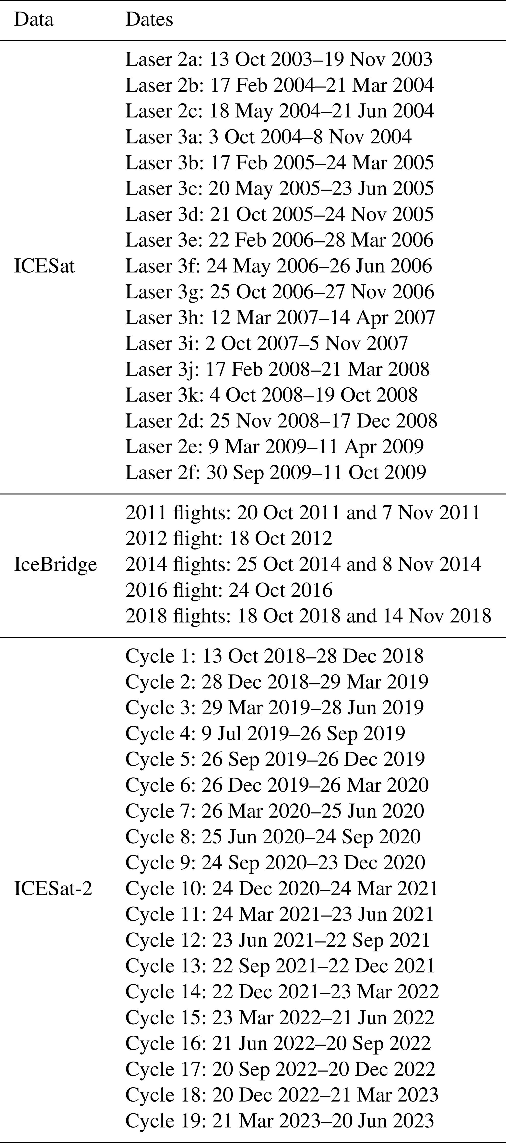
For lakes where observed elevation changes significantly deviate from their outlines defined in existing inventory, a repeat-track analysis is performed to investigate the spatial pattern of these deviations. The analysis utilizes ICESat-2 ATL11 data, which are repeatedly collected over different cycles through three pair tracks (PT1, PT2, PT3), as illustrated in Fig. 2, along each Reference Ground Track (RGT). All track data are then differenced with the reference DEM synthesized in this study, yielding elevation changes for each track in each cycle to verify the updated outlines.

3.2.3 Obtaining elevation changes of subglacial lakes from 2003 to 2023 using multi-mission altimetry data

To capture the long-term dynamic variations of active subglacial lakes in the RIS and gain a comprehensive understanding of subglacial hydrological patterns, altimetry data from ICESat (2003–2009), IceBridge (2011–2018), and ICESat-2 (2018–2023) are combined to calculate surface elevation changes for each active subglacial lake. As described earlier, surface elevation changes are derived by subtracting ICESat, IceBridge, or ICESat-2 altimetry data from their corresponding values in the reference DEM. To isolate elevation variations predominantly attributable to subglacial water activity from regional surface elevation trends (such as glacier melting and accumulation), this study adopts the method proposed by Siegfried et al. (2014), which involves subtracting the average exterior lake measurements from the average interior lake measurements based on the delineated outlines of subglacial lakes. Moreover, we propose a weighting method that assigns weights to measurement points based on their distance from the lakes' outlines to calculate surface elevation changes in subglacial lakes accurately. Generally, for measurements within the lake, the farther a measurement point is from the lake's outline, the stronger the correlation between ice surface elevation changes and subglacial lake activity. Conversely, for measurements outside the lake, the farther the point is from the outline, the weaker this correlation. The surface elevation changes are calculated by using Eq. (1).

$$\begin{array}{}\text{(1)}& \mathrm{\Delta }h=\mathrm{\Delta }{h}_{\mathrm{inlake}}-\mathrm{\Delta }{h}_{\mathrm{outlake}}={\displaystyle \frac{{\displaystyle }\sum _{i=\mathrm{1}}^{N_{\mathrm{in}}}{p}_i{h}_i}{{\displaystyle }\sum _{i=\mathrm{1}}^{N_{\mathrm{in}}}{p}_i}}-{\displaystyle \frac{{\displaystyle }\sum _{j=\mathrm{1}}^{N_{\mathrm{out}}}{p}_j{h}_j}{{\displaystyle }\sum _{j=\mathrm{1}}^{N_{\mathrm{out}}}{p}_j}},\end{array}$$

where Δh_inlake represents the elevation changes for lake interior points. Δh_outlake represents the elevation changes for lake exterior points. N_in, N_out denote the quantities of lake interior and exterior points respectively. p_i, p_j correspond to the weights, which are assigned based on the minimum distance from the elevation measurement points to the lake outline, and are normalized to sum to 1 for the interior and exterior points separately. h_i and h_j correspond to elevation change values for lake interior and exterior points. To comprehensively investigate the spatiotemporal evolution of these lakes, we construct elevation change time series for each group by integrating multi-source altimetry data from ICESat, IceBridge, and ICESat-2. Following Siegfried and Fricker (2018), we normalize the elevation changes to ensure data comparability and facilitate analysis: all data are adjusted by subtracting the elevation change value at the initial ICESat observation time, making each time series curve start from zero. This normalization facilitates comparison of variation patterns across different lakes and time periods.

To characterize the filling-draining dynamics of lakes between adjacent observation months, we conduct a quantitative analysis of volume changes for each lake. Assuming the subglacial lake outlines remain constant, we estimate the volume changes of each subglacial lake using the following approach:

$$\begin{array}{}\text{(2)}& \mathrm{\Delta }V=A\times \mathrm{\Delta }h,\end{array}$$

where ΔV is the volume change, A is the lake area calculated based on the lake outline, and Δh is the weighted average elevation change derived from altimetry data.

The uncertainty in volume change is obtained by combining the uncertainty in lake-induced surface elevation change with the uncertainty in lake area. The detailed calculation is described in the Supplement. Furthermore, as Stubblefield et al. (2021) point out, altimetry-derived estimates of subglacial volume change can deviate considerably from their true values due to viscous ice flow. For a given ice thickness and basal drag, shorter filling–draining periods lead to altimetry-derived volume changes that more closely match the true subglacial volume changes (Stubblefield et al., 2021). Following the approach of Stubblefield et al. (2021), and using parameter values appropriate for the RIS, we estimated the ratio of altimetry-derived volume change to the true volume change ($\mathrm{\Delta }{V}_{\mathrm{est}}/\mathrm{\Delta }{V}_{\mathrm{true}}$). The results are presented in Fig. S1 in the Supplement, and the quantitative statistics for all subglacial lakes within the RIS are summarized in Table S2 in the Supplement.

3.3 The detailed trend of elevation changes within lakes based on crossover analysis

The elevations at crossovers obtained from ascending and descending tracks, with the time interval approximately from one to several tens of days, are compared to reveal the detailed elevation change patterns in different regions of the lake.

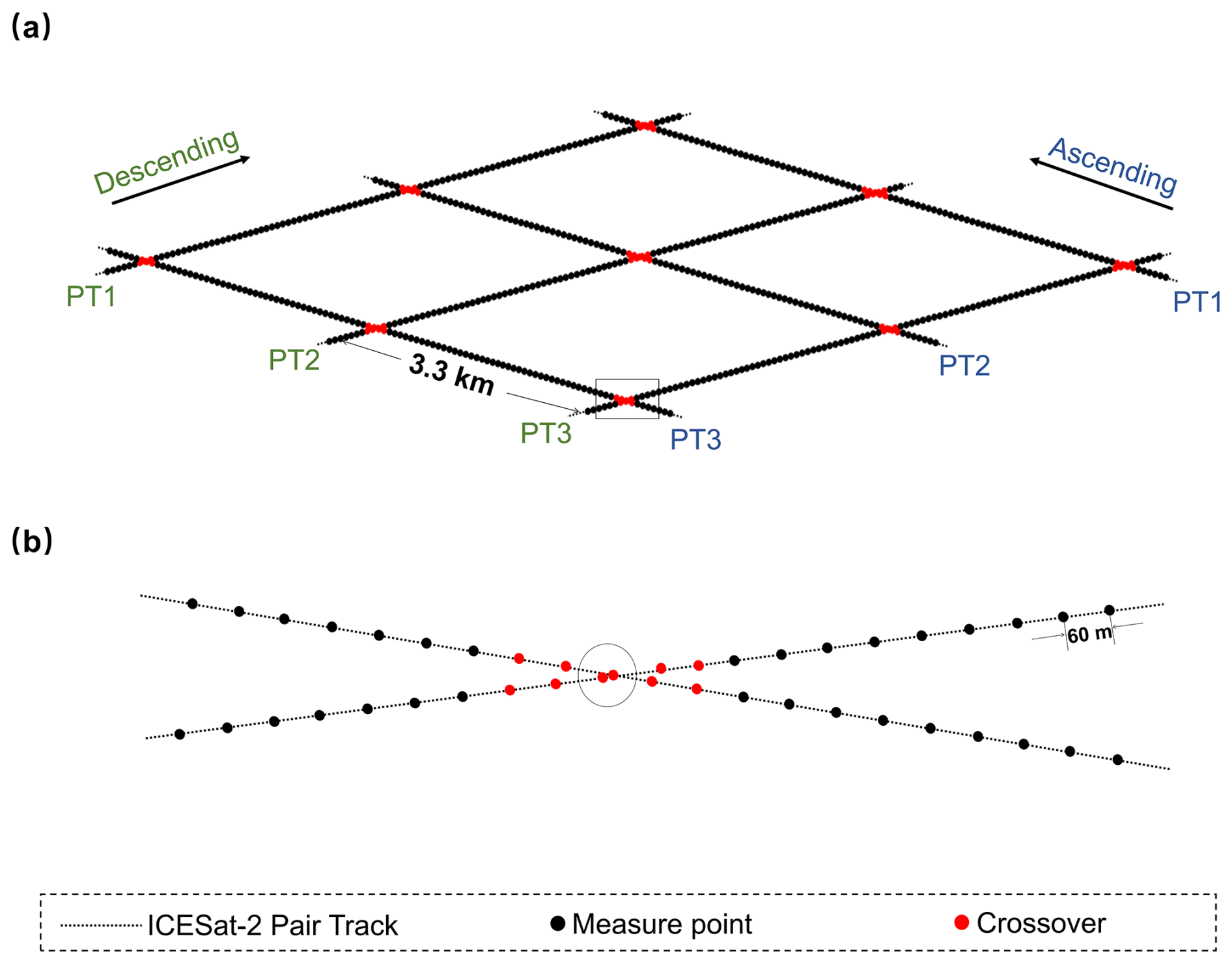
Figure 2 A schematic diagram of crossovers in ICESat-2 ATL11 data. (a) Distribution of crossovers at the intersections of ascending and descending reference ground tracks (RGTs), where each RGT consists of three pair tracks (PTs) spaced 3.3 km apart. The magnified view of crossovers within the box in (a) is shown in (b).

In the altimetry data from ICESat-2, each measurement point is treated as the center of a circular search area with a radius of 65 m, within which neighboring measurement points are identified. If a measurement point from a crossing track is found within this range, it is recorded as a crossover stored in ATL11 data products. However, in our study area, multiple crossovers, forming X-shaped clusters as illustrated in Fig. 2a, can be found in a pair of ascending and descending tracks. This is because large intersection angles between ascending and descending tracks at high latitudes allow a single crossing track to match multiple crossovers. To address this, we first identify the two measurement points closest to the theoretical intersection of the ascending and descending tracks within each crossover cluster, as shown by the two points inside the circle in Fig. 2b. Next, we compare the number of valid data points associated with these measurements and select the point with the greater number of valid data points as the representative crossover. This point is then used to analyze elevation changes at the crossover. We organize the elevation measurement data at a crossover in chronological order. Then, the earliest elevation measurement value at time T₀ is subtracted from the elevation values at each moment T_i to calculate the elevation change at each moment relative to the initial time. Finally, the elevation changes for each crossover are arranged into time series.

3.4 Subglacial hydrological analysis in the RIS

To explore the hydrological connections between subglacial lakes in the RIS region, the subglacial hydraulic potential ϕ is calculated using the Shreve hydraulic potential model (Shreve, 1972), as shown in Eq. (3).

$$\begin{array}{}\text{(3)}& \mathit{\varphi }=B+{\displaystyle \frac{{\mathit{\rho }}_{\mathrm{i}}}{{\mathit{\rho }}_{\mathrm{w}}}}H,\end{array}$$

where ρ_w and ρ_i represent the densities of water (1000 kg m⁻³) and ice (917 kg m⁻³), respectively. B and H denote the bedrock elevation and ice thickness, respectively, which are obtained from BedMachine v3 in this study. First, based on the results of the hydraulic potential calculations, the hydraulic potential surface is generated in ArcGIS. Then, the D8 flow direction method (O’Callaghan and Mark, 1984) is employed to calculate the changes in hydraulic potential gradients in each direction within each grid cell, directing flow to the direction of the steepest hydraulic potential gradient, thereby determining the subglacial drainage networks. Finally, according to the Strahler (Strahler, 1957) method, all river systems are classified into hierarchical networks from first to sixth orders based on the calculated cumulative flow from the largest to the smallest, simulating the final configuration of the subglacial hydrological networks.

4 Results

4.1 Outlines of active subglacial lakes in the RIS region

In this subsection, we delineate the outlines of active subglacial lakes in the study area based on elevation change results during the ICESat-2 mission period. Among the nine previously reported subglacial lakes, four remain active during this period, while five show no significant filling or drainage signals. In addition, 14 newly detected subglacial lakes are identified. A detailed description of these three categories of subglacial lakes is provided below.

Of the nine reported subglacial lakes, lakes Rec1, Rec2, Rec4, and Rec6 demonstrate noticeable filling-draining cycles during the ICESat-2 mission. However, the draining and filling areas of these four lakes during this time period show differences from those in the inventory. The updated outlines and the annual elevation changes of lakes Rec1, Rec2, Rec4, and Rec6 are shown in Fig. 3.

Figure 3 Updated outlines and the annual elevation changes of lakes (a) Rec1, (b) Rec2, (c) Rec4, and (d) Rec6.

Our repeat-track analysis confirms the asynchronous variations within lake Rec1 identified during the ICESat-2 mission. The quantitative analysis reveals that different parts of the lake exhibit contrasting elevation change patterns, with substantial differences in both magnitude and timing. Specifically, according to the elevation change ranges during the time periods of these three repeat tracks (RGT 0063 PT3, RGT 0505 PT2, and RGT 0947 PT1) from Cycle 3 to Cycle 19 (Fig. 4b–d), the elevation changes of the west part of lake Rec1 (approximately 3 m) are significantly greater than those of the east part of lake Rec1 (approximately 0.5 m). There are even periods when the elevation changes are reversed. For example, the west part of lake Rec1 is draining while the east part is filling during Cycle 3, and this situation is reversed in Cycle 17, as shown in Fig. 4b–d. Therefore, we recognize lake Rec1 as two separate lakes, named as Rec1-1 (west part of lake Rec1) and Rec1-2 (east part of lake Rec1) during the ICESat-2 mission, as shown in Fig. 3. It is worth noting that the boundary zone between the outlines of these two parts contains transitional elevation signals that create uncertainty. Therefore, we maintain a gap between the lake sections, which represents a conservative approach to avoid incorrectly classifying the transition area as part of either lake.

Figure 4 Repeat-track analysis results of lake Rec1. (a) The location of three repeat tracks crossing through lake Rec1. (b)–(d) show the elevation changes of individual cycles along each repeat track, as well as the overall elevation change range (cyan line, right y axis) for (b) RGT 0063, (c) RGT 0505, and (d) RGT 0947. The varying widths of the gaps between the gray zone (Rec1-1 and Rec1-2) in (b)–(d) are caused by slightly different placements among the three ICESat-2 tracks.

As illustrated in Fig. 3, lake Rec2's outline contracted inward while preserving its central location, evolving into a more elongated form. The shape and position of lake Rec4 have also changed, developing a more elongated morphology, with a subtle displacement in the lake's center position. Lake Rec6 displayed two sections with contrasting elevation change patterns during the ICESat-2 mission, leading us to classify them as separate lakes: lake Rec6-1 (west section) and lake Rec6-2 (east section), as shown in Fig. 3.

The remaining five reported lakes (Rec3, Rec5, Rec7, Rec8, and Rec9) show low levels of activity during the ICESat-2 period, with slight elevation changes (less than 0.5 m; see Fig. S2 for their outlines and annual elevation changes), and therefore, they are not further analyzed in this study. In addition, 14 active subglacial lakes, named lakes RecN1 through RecN14 from downstream to upstream, are newly detected in this study (see Figs. S3–S5). The spatial distribution of these newly detected subglacial lakes and updated subglacial lakes (Rec1-1, Rec1-2, Rec2, Rec4, Rec6-1, and Rec6-2) is illustrated in Fig. 1.

4.2 Analysis of time series of elevation changes of subglacial lakes

In this subsection, we reveal the cyclical filling-draining patterns of all active subglacial lakes in the study area using multi-source altimeter data from 2003 to 2023. Based on their spatial distribution, these lakes are categorized into lower trough, upper trough, and upstream of bedrock trough groups for detailed analysis.

According to Fricker et al. (2014), the bedrock trough in the RIS region is naturally divided into upstream and downstream sections by a ridge located at −17° W. Based on the geographical distribution of active lakes in the region (as shown in Fig. 1), we classified all the lakes into three groups: The first group (lakes RecN1, RecN2, RecN3, RecN4, Rec1-1, Rec1-2, Rec2, and Rec3) is located in the downstream section of the bedrock trough; the second group (lakes RecN5, RecN6, RecN7, RecN8, Rec4, Rec5, Rec6-1, and Rec6-2) is concentrated in the upstream section of the bedrock trough; and the third group (lakes RecN9, RecN10, RecN11, RecN12, RecN13, RecN14, Rec7, Rec8, and Rec9) is primarily distributed in the upstream region outside the bedrock trough, exhibiting relatively dispersed spatial characteristics. The time series in Figs. 5–7 represent the weighted average elevation change across the entire lake region, including lower/upper troughs and upstream of bedrock trough. These time series curves intuitively reflect the hydrological dynamic characteristics of the lakes: an upward trend indicates rising water levels during the filling phase, while a downward trend signifies decreasing water levels during the draining phase.

4.2.1 Lower trough

The temporal elevation changes of active lakes in the lower trough are shown in Fig. 5. During the ICESat mission, lakes Rec1-1 and Rec1-2 exhibit the most significant elevation changes: lake Rec1-2 shows a nearly continuous filling trend from early 2003 to 2008, with a cumulative rise exceeding 5.5 m, while lake Rec1-1 experiences a notable filling event between May 2004 and May 2005, with an elevation increase of over 3 m. During the same period, lakes RecN4 and Rec2 also demonstrate significant dynamic features, with elevation changes exceeding 2 m. In contrast, lakes Rec3, RecN1, RecN2, and RecN3 show relatively minor elevation changes, with fluctuations around 1 m.

During Operation IceBridge, lake RecN2 shows particularly significant variations, with elevation dropping sharply by over 10 m between October 2011 and October 2012, and then showing an overall elevation increase of approximately 9 m when measured again in October 2018. During the same period, lake Rec3 also experiences significant elevation changes, with an increase of up to 7 m. Lake Rec1-1 exhibits a pattern of first accumulating water and then draining, with a maximum elevation change of approximately 4 m. Lakes Rec1-2 and Rec2 initially experience slight drainage before stabilizing. Lakes RecN1 and RecN3 remain relatively stable during this period. Lake RecN4 has only one observation recorded in October 2011, with an elevation approximately 1.5 m higher than that measured by ICESat in October 2009, and similar to the elevation measured by ICESat-2 in October 2018. Additionally, the observations from IceBridge in October 2018 show high consistency with ICESat-2 data from the same period, providing reliable connecting data for elevation changes and further confirming the reliability of the observational data.

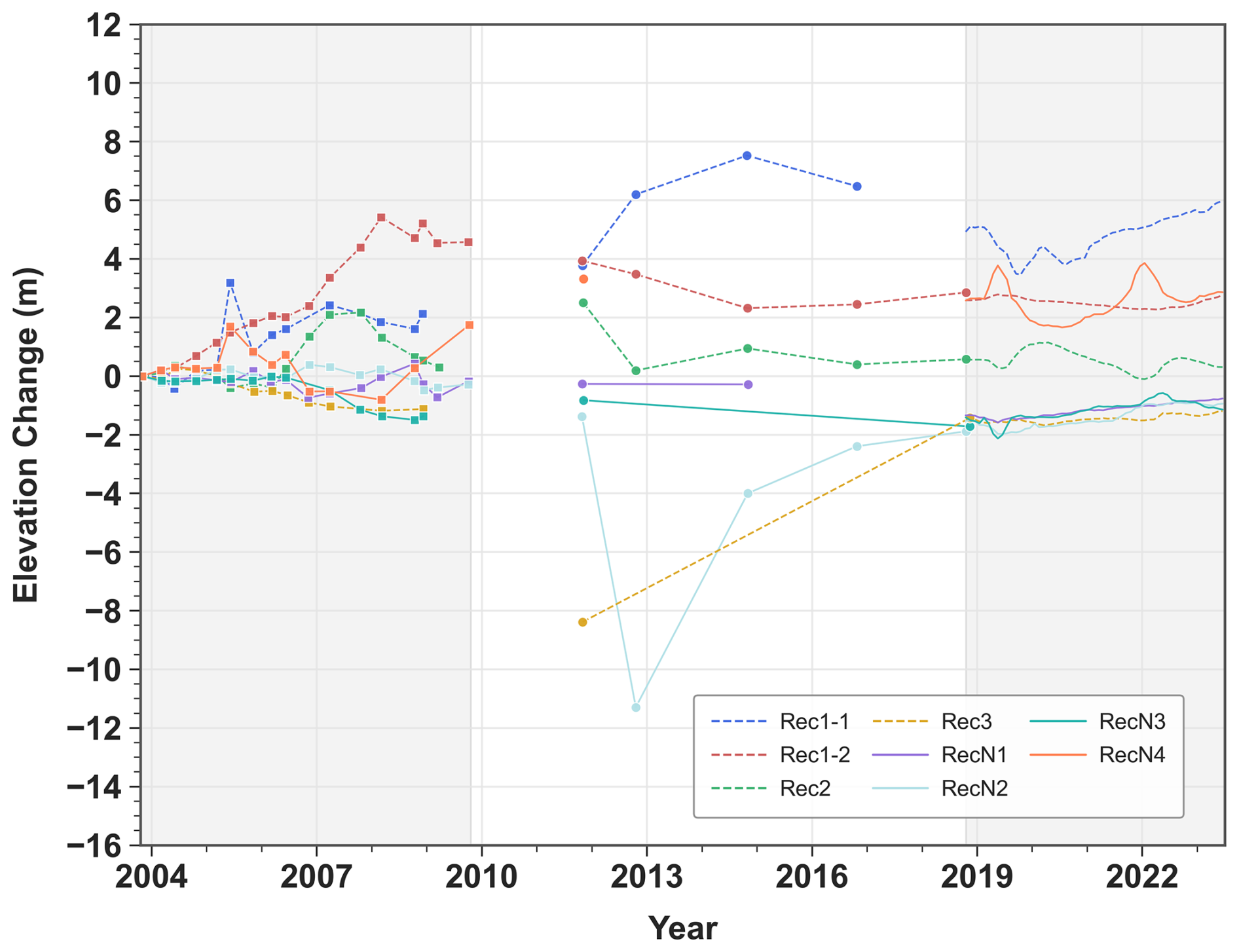
Figure 5 Time series of elevation changes of the lakes in the lower trough. Individual observations are shown as markers for ICESat (2003–2009, squares) and IceBridge (2011–2018, circles). For ICESat-2 (2018–2023), monthly elevation changes are calculated using a three-month temporal window and displayed as connected lines due to the higher temporal resolution.

During the ICESat-2 observation period, lakes RecN4, Rec1-1, and Rec2 show significant elevation changes with distinct drainage and recharge events. Lake RecN4 experiences two notable filling-draining cycles. The first cycle begins in February 2019, with elevation rising by 1.1 m within three months, followed by a rapid decrease to its lowest point in July 2020, with a total decline of 2.1 m. The second cycle occurs between July 2020 and October 2022, initially experiencing an increase of approximately 2.4 m, reaching its peak in January 2022, followed by another decline of about 1.4 m by October 2022. Lake Rec1-1 undergoes two draining-filling cycles. Notably, between August 2020 and June 2023, a nearly continuous elevation uplift is observed with a cumulative increase of 2.2 m. Lake Rec2 experiences two filling-draining cycles. The first cycle commences in June 2019, with a gradual water accumulation of 0.9 m over a 10-month period. By April 2020, the lake transitions to a sustained drainage phase, culminating in a cumulative decrease of approximately 1.3 m by January 2022. The second cycle begins in January 2022, with elevation rising by 0.6 m over the subsequent eight months until September 2022. Finally, from September 2022 through June 2023, Lake Rec2 persists in its draining trend, exhibiting an elevation decrease of 0.3 m. Lake Rec1-2 maintains relative stability during this period, showing an overall trend of initial decrease followed by increase. Lakes RecN1, RecN2, and RecN3 display similar change patterns: decreasing in elevation from October 2018 to June 2019, then transitioning to a fluctuating upward trend. The total elevation changes range from 0.5 to 1 m. Lake Rec3 exhibits relatively stable characteristics during this period, with minimal elevation changes.

4.2.2 Upper trough

The time series analysis of elevation changes for subglacial lakes in the upper trough is presented in Fig. 6. During the ICESat mission period, lakes Rec6-1 and Rec6-2 show the most significant changes. Lake Rec6-1 experiences intense drainage between early 2006 and early 2008, featuring a sustained elevation decrease exceeding 10 m. The elevation change pattern of lake Rec6-2 can be divided into two phases: between 2003 and 2006, it shows similar change trends to lake Rec6-1, while from early 2008 to late 2009, it displays distinct dynamic characteristics, with four significant elevation change events recorded, each exceeding 4 m in magnitude. Lake Rec4 also exhibits significant hydrological activity, recording multiple major recharge and drainage events with amplitudes exceeding 1 m. In contrast, lakes Rec5, RecN5, and RecN7 show relatively moderate change characteristics: lake Rec5's elevation displays a fluctuating slow rise with total amplitude less than 1 m; lake RecN5 overall undergoes a fluctuating drainage process with a cumulative elevation decrease of 0.8 m; while lake RecN7 records a fluctuating rise of approximately 0.8 m. Lakes RecN6 and RecN8 exhibit similar elevation change characteristics throughout the observation period. Lake RecN6 first experiences a cumulative elevation decrease of about 1 m from late 2003 to late 2006; then undergoes a six-month rise-and-fall cycle with comparable amplitudes; subsequently enters a two-year recharge period with an elevation increase of 0.7 m; and finally shows fluctuations of about 0.5 m. Lake RecN8 shows similar patterns to lake RecN6, with only relatively smaller magnitudes of change.

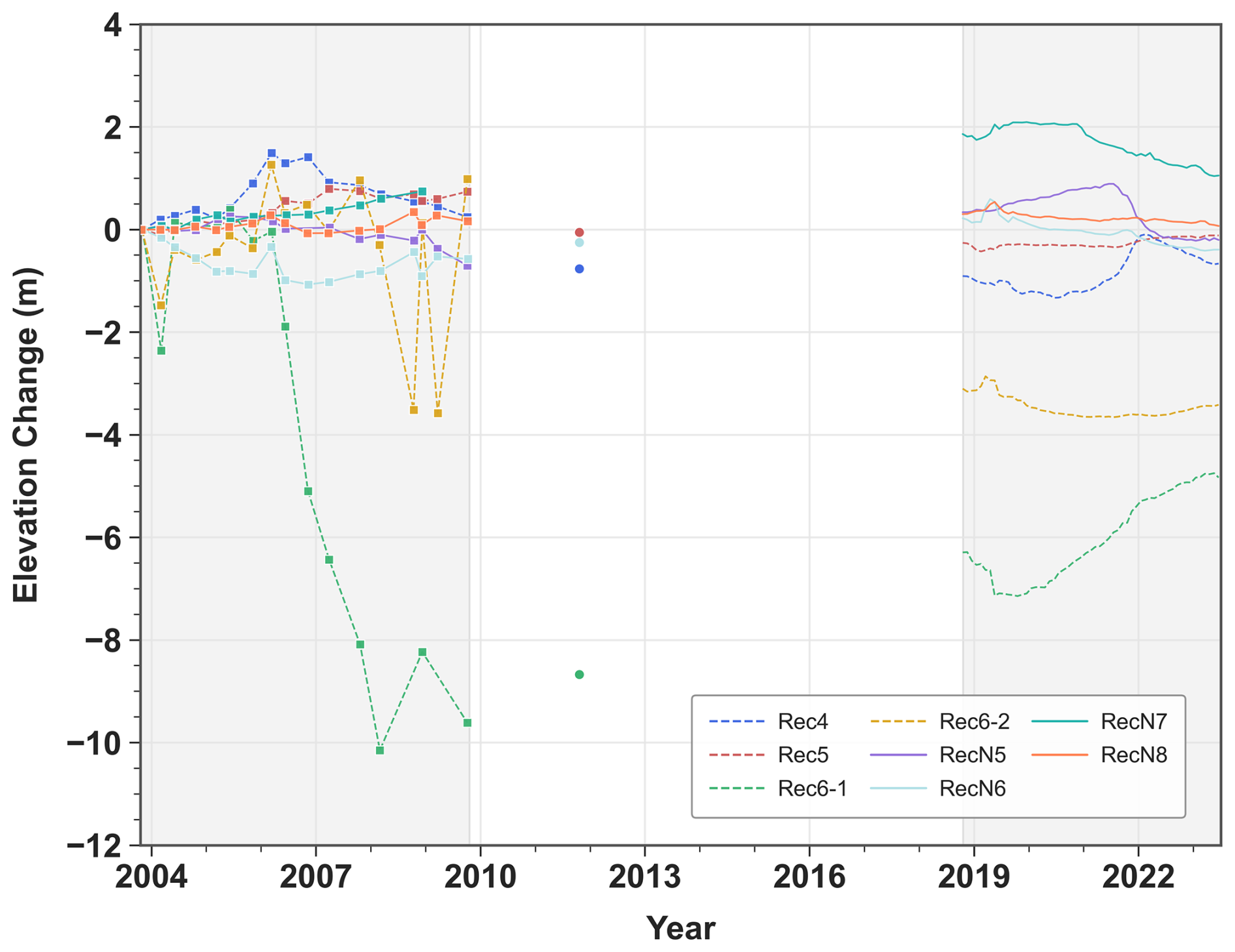
Figure 6 Time series of elevation changes of the lakes in the upper trough, with a similar setting as Fig. 5.

During the Operation IceBridge observation period, only lakes Rec4, Rec5, Rec6-1, and RecN6 are observed once in 2011. Compared to the elevations measured by ICESat in late 2009, lakes Rec4 and Rec5 experience a decrease of approximately 1 m, while both lakes Rec6-1 and RecN6 experience elevation increases, with rises of approximately 1 and 0.5 m, respectively. Compared to the elevation data observed by ICESat-2 in late 2018, the elevations of lakes Rec4, Rec5, and RecN6 show no significant changes (less than 0.5 m), while lake Rec6-1 exhibits a substantial increase of more than 2 m.

During the ICESat-2 observation period, lakes Rec6-2, RecN6, RecN7, and RecN8 initially show similar change patterns, successively reaching their peak elevations during May–June 2019. However, these lakes subsequently exhibit distinct change patterns: lakes RecN6 and RecN8 immediately enter continuous drainage modes, lake Rec6-2 stabilizes after approximately two years of drainage, while lake RecN7 maintains its peak elevation until January 2021 before beginning to decline, recording a cumulative decrease of over 1 m by the final observation in June 2023. Lake Rec6-1, as the most active lake in the region, displays a distinct change pattern compared to other lakes. Prior to May 2019, while other lakes are generally in filling phases, lake Rec6-1 exhibits continuous drainage characteristics. Subsequently, after May 2019, it transitions to a sustained filling mode accompanied by minor fluctuations. Lake Rec4 records a complete draining-filling-draining cycle: experiencing fluctuating drainage from late 2018 to May 2019 with an elevation decrease of approximately 0.5 m; then entering a sustained filling phase with gradual water level rise until reaching its peak in early 2022, accumulating an increase of about 1.5 m; finally entering a new drainage phase with an elevation decrease of approximately 0.6 m. Lake RecN5 shows a significant elevation increase of 0.6 m during the period from October 2018 to July 2021; subsequently experiences a drainage event between July 2021 and May 2022, with a sharp elevation decrease of 1.2 m; and finally enters a relatively stable period from May 2022 to June 2023, showing no significant changes. Lake Rec5 exhibits remarkable stability throughout the observation period, maintaining elevation changes within 0.3 m.

4.2.3 Upstream of bedrock trough

As shown in Fig. 7, the subglacial lakes in the upstream region of the bedrock trough exhibit different dynamic characteristics during various observation periods. During the ICESat mission period, lakes Rec7, Rec8, and RecN11 exhibit significant elevation changes. Lake Rec7 shows a nearly continuous declining trend with a cumulative decrease of 1.5 m; lake Rec8 experiences two distinct phases: initially showing minimal elevation changes, followed by a sharp decline of 3.6 m between March 2006 and February 2008; lake RecN11 demonstrates elevation changes exceeding 1.5 m during single filling or draining events. Lake RecN10 maintains relative stability during the early observation period, showing only one significant fluctuation from late 2008 to early 2009, characterized by a decrease followed by an increase, with both changes approaching 1 m in magnitude. Lakes Rec9, RecN9, RecN12, RecN13, and RecN14 maintain relatively stable conditions, with elevation changes limited to around 0.5 m.

Although the lakes in this area are not covered by IceBridge data, by comparing the latest ICESat data with the earliest ICESat-2 data, it is found that the elevations of lakes Rec7, Rec8, Rec9, RecN9 and RecN14 are similar. In contrast, the elevations of lakes RecN10, RecN11, and RecN12 decrease by approximately 4, 5, and 2.5 m, respectively, while the elevation of lake RecN13 increases by about 1.5 m.

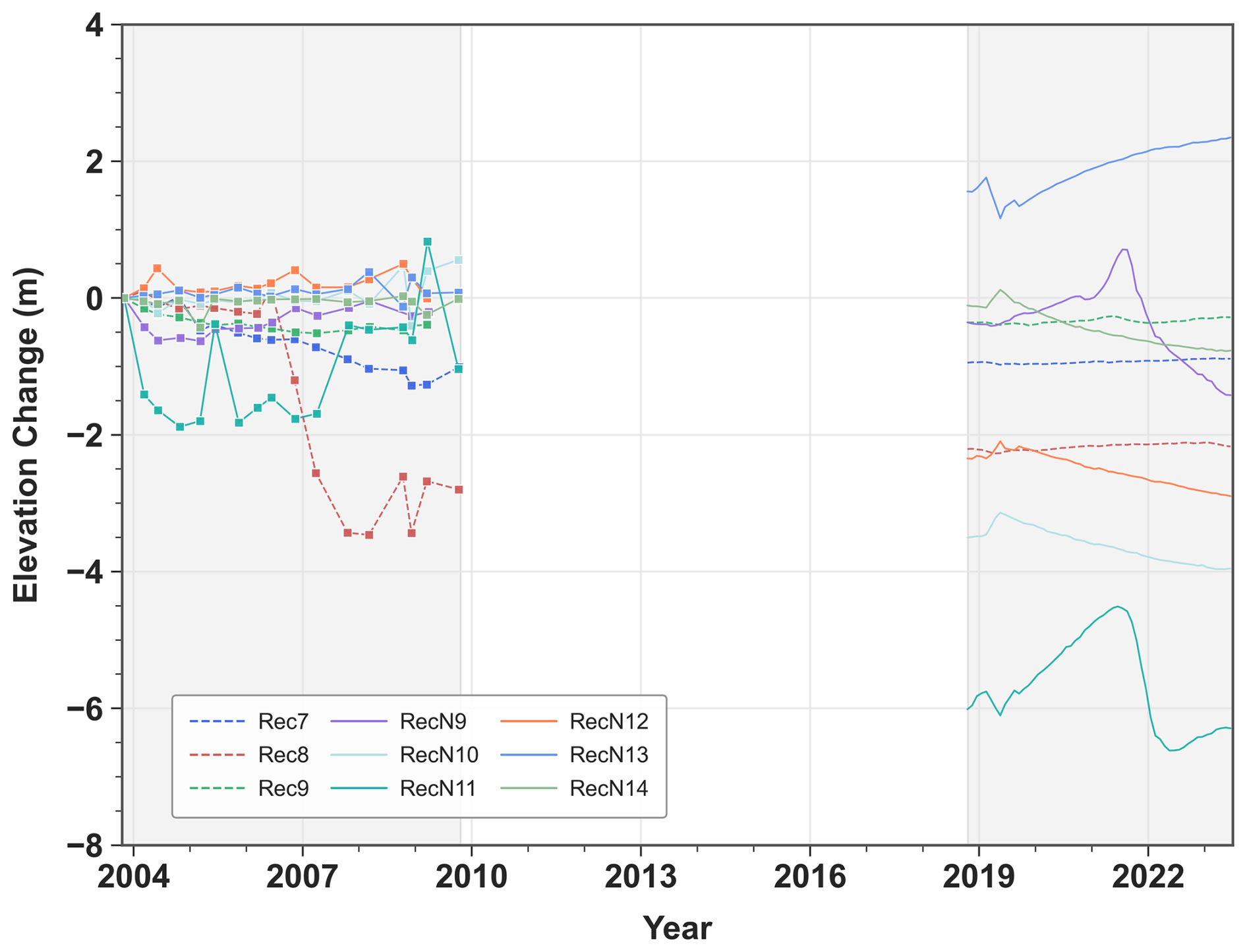
Figure 7 Time series of elevation changes of the upstream lakes, with a similar setting as Fig. 5.

During the subsequent ICESat-2 mission period, lake RecN9 experiences significant elevation changes, first rising by 1.1 m followed by a decrease of 2.1 m; lakes RecN10, RecN12, and RecN14 display highly consistent change patterns, all reaching peak elevations around May 2019 before continuously declining by approximately 0.8 m; lakes RecN13 and RecN11 initially show similar change trends, with lake RecN13 reaching its lowest point in May 2019 (dropping by 0.6 m) before gradually rising by 1.6 m, while lake RecN11 undergoes a significant transformation after July 2021, rapidly declining by 2.1 m followed by a slow recovery trend. Lakes Rec7, Rec8, and Rec9 show notably reduced activity during this period, maintaining relatively stable elevation changes.

We analyze lakes by clustering them based on their geographic locations and find that some lakes within the same cluster (such as lakes RecN7 and RecN8 in the upper trough region, lakes RecN2 and RecN3 in the lower trough region, and lakes RecN9 and RecN11 in the upstream region) exhibit similar elevation change patterns, indicating a certain degree of regional hydrological consistency. However, lakes within the same region do not change in perfect synchrony, and these differences likely stem from the heterogeneity of basal topography. The hydrological network of the Recovery Ice Stream is strongly controlled by bedrock topography (Fricker et al., 2014), which may lead to different hydrological connectivity pathways even between lakes in close geographic proximity. Therefore, we hypothesize that the hydrological patterns of lakes in the RIS, under the influence of basal topographic features, form a complex hydrological connectivity network, causing lakes to exhibit both a degree of cluster similarity in space while maintaining their unique hydrological characteristics. A more detailed bedrock topography may help to reveal the synchronical pattern of regional draining/filling behavior of lakes, which shall satisfy the mass conservation principle more strictly.

4.3 The detailed trend of elevation changes within the lakes based on crossover analysis

To investigate the detailed elevation change trend within the subglacial lakes, we select four representative lakes based on their characteristic temporal variations. The results reveal significant spatial heterogeneity within individual lakes, with maximum elevation changes consistently occurring in central areas and minimal changes in peripheral regions.

Lake Rec6-1, which demonstrates the most pronounced elevation change amplitude in long-term observations, is selected. Additionally, lake Rec6-2, which was part of the same lake as Rec6-1 in the past, is also investigated to facilitate a detailed comparison of the elevation change patterns between these two adjacent lakes. Lake Rec2 is geographically adjacent to the Shackleton Range, with its hydrological activity influenced by the topography of the Shackleton Range (Fricker et al., 2014). Considering its geographical significance, it is analyzed as a representative case. Lake RecN4 exhibits highly pronounced filling-draining cycle characteristics in its temporal elevation changes, with each complete filling-draining cycle lasting approximately 2 years and an elevation change range of about 2 m, as shown in Fig. 5. Therefore, it is also analyzed as a representative active subglacial lake. As shown in Fig. 8, in each subplot, every line represents the elevation change time series of a crossover, with color intensity related to the normalized magnitude of elevation change (darker colors indicate larger changes). Meanwhile, in the insets of each subplot, the spatial distribution of crossovers within each lake is displayed using exactly the same colors as their corresponding time series curves. Additionally, it can be observed from the figure that the thick black dashed lines (weighted average results) show consistent trends with individual crossover curves and are located near the median range of all crossover results.

As shown in Fig. 8a, the elevation of subglacial lake Rec6-1 exhibits a continuous increasing trend during the ICESat-2 observation period, indicating significant active characteristics. Although all crossovers display similar patterns of elevation change, their magnitudes show notable spatial variations: crossovers in the central lake area demonstrate the maximum elevation changes, while those distributed in the peripheral regions show smaller changes. By June 2023, this spatial differentiation reaches its most pronounced level, with maximum elevation changes exceeding 4 m in the central lake area, while the minimum elevation changes in the peripheral regions are only about 0.3 m.

Lake Rec6-2 shows different characteristics of elevation change during the ICESat-2 observation period. The elevation of crossovers in lake Rec6-2 initially decreases and then stabilizes as shown in Fig. 8b. In particular, between May 2019 and May 2021, these two lakes show opposite activity patterns, with lake Rec6-1 in a phase of continuous water recharge and lake Rec6-2 in a drainage process. This difference indicates that the original lake Rec6 evolves into two parts.

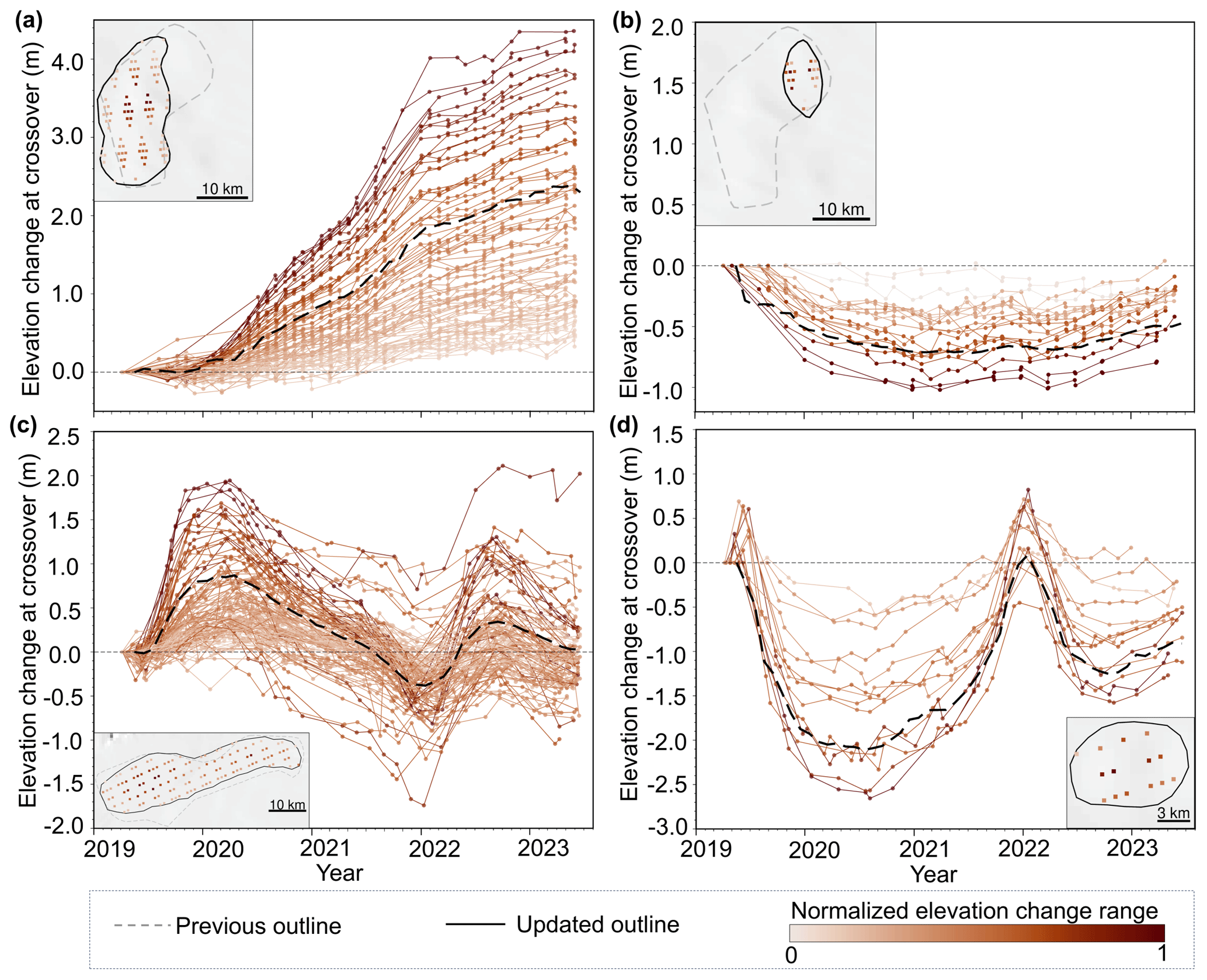
Figure 8 The detailed trend of elevation changes of lakes (a) Rec6-1, (b) Rec6-2, (c) Rec2, and (d) RecN4. The locations of crossovers in each lake are shown in the inset, with their colors indicating the corresponding normalized elevation change range. The thick black dashed lines represent the weighted average elevation changes of the lakes calculated using the method in Sect. 3.2.3.

Lakes Rec2 and RecN4 exhibit distinct filling and draining characteristics. Based on the spatial distribution of crossovers and the temporal elevation change patterns shown in Figs. 8c, d, crossovers in the central areas of the lakes display significant elevation changes, whereas those in the peripheral areas exhibit minimal variation, remaining close to 0. As shown in Fig. 8c, lake Rec2 is a large and elongated lake with extensive crossover observation data. During the ICESat-2 observation period, the lake undergoes two filling-draining cycles, with elevation changes at crossovers remaining within the range of 4 m. The first filling-draining event takes place from May 2019 to February 2021. During the filling phase, most crossovers reach their peak elevation in March 2020, when the elevation difference between crossovers in the central and peripheral regions exceeds 2 m. Subsequently, during the approximately two-year-long draining phase, the elevations at crossovers gradually decrease, reaching their lowest values in February 2022. The second filling-draining event spans from February 2022 to June 2023. By September 2022, the elevations at crossovers reach a second peak. This period also marks the stage with the most pronounced elevation differences, as the elevation difference between the central and peripheral crossovers exceeds 2.5 m. As shown in Fig. 8d, Lake RecN4 is a relatively small lake with fewer crossovers in its observation data. During the study period, the lake experiences two draining-filling cycles. The first draining-filling event has a longer duration, spanning from May 2019 to January 2022. During this period, the crossover elevations decrease until August 2020, achieving their minimum values, with the largest elevation decrease of 2.8 m observed in the central region of the lake, while the elevation decrease in the peripheral region is relatively small at only 0.6 m, resulting in an elevation difference of over 2 m between the central and peripheral regions. The second draining-filling event occurs between January 2022 and June 2023. The crossover elevations within the lake reach their second trough in September 2022, during which the elevation difference between the central and peripheral regions exceeds 1 m.

4.4 Hydraulic potential and hydrology of the RIS

Based on hydraulic network simulation, we analyzed the relationship between filling and drainage for active subglacial lakes located along the primary drainage pathways. It is indicated that effective hydraulic connectivity can be established between subglacial lakes in the RIS, exhibiting upstream-downstream hydrological connections during different observation periods.

The simulated hydrological networks, as shown in Fig. 9a, are obtained according to the subglacial hydrological analysis. It is found that most of the subglacial lakes are situated along the simulated subglacial hydrological networks, affirming that the active subglacial lakes within the RIS form a hydrologically connected subglacial water system. Based on the Strahler (Strahler, 1957) method, we classify the hydrological network into six distinct orders. Subglacial water flows along these streams, gradually converging from lower order streams to higher order streams, with the flow becoming progressively stronger. In this study, we focus on the activity of eleven active subglacial lakes (blue areas in Fig. 9a) located along highest-order and second-highest-order stream networks. These networks constitute the primary drainage pathways within the system, forming the main trunk channels where subglacial water from extensive upstream catchments converge, resulting in maximized water fluxes. From upstream to downstream, these subglacial lakes are sequentially arranged as lakes RecN10, Rec9, RecN9, RecN6, Rec6-2, Rec6-1, Rec4, RecN4, RecN2, Rec1-2, and RecN1. By calculating the volume differences between adjacent observation months, we establish diagnostic criteria for lake draining and filling status: a positive volume difference indicates a filling process, while a negative volume difference indicates a draining process. Figure 9b and c show histograms of volume differences for these eleven subglacial lakes during adjacent observation months throughout the ICESat and ICESat-2 missions, respectively. The lakes from upstream to downstream are marked using a color gradient transitioning from dark to light hues. Due to the significant sparsity of valid altimetry data obtained during the IceBridge mission, a detailed discussion is not conducted for this period.

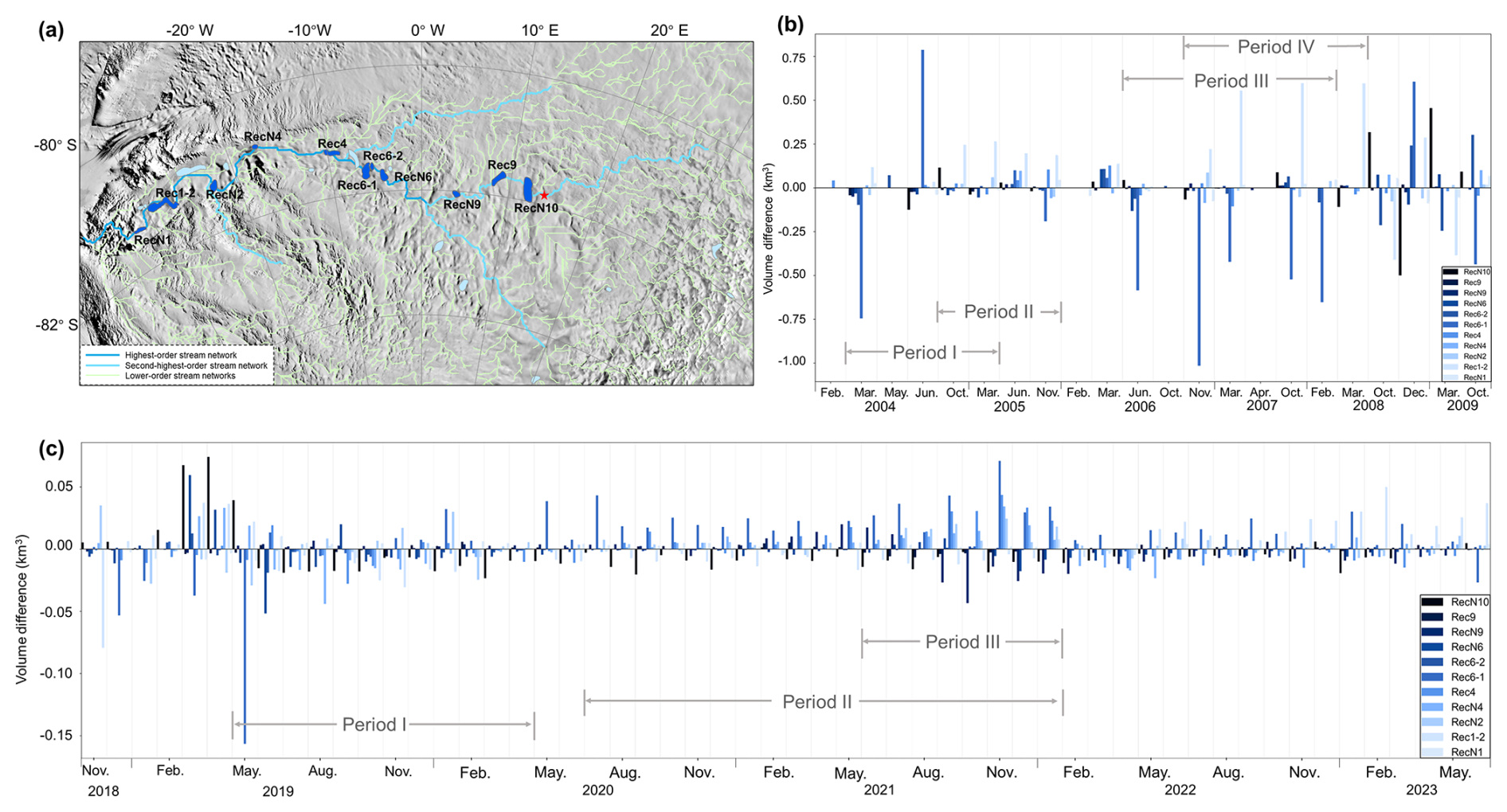
Figure 9 (a) The simulated distribution of hierarchical hydrological networks in the subglacial hydrological system. (b) and (c) present the histograms of volume differences between adjacent observation months of eleven lakes along the highest-order and second-highest-order stream networks during ICESat and ICESat-2 missions, respectively.

The volume change uncertainties for individual lakes are presented in Table S1. During the ICESat mission period (from February 2004 to October 2009), the subglacial hydrological system of RIS shows a total discharge of 8.91±0.56 km³, a total recharge of 8.75±0.55 km³, and a net water volume change of $-\mathrm{0.16}\pm \mathrm{0.78}$ km³, indicating that the RIS hydrological system releases a certain amount of water during this period. From March 2004 to March 2005 (Period I in Fig. 9b), the upstream system is predominantly characterized by discharge, with a cumulative water release of approximately 1.52±0.29 km³, while the downstream region between October 2004 and November 2005 (Period II in Fig. 9b) exhibits a recharge-dominant state, accumulating approximately 1.62±0.29 km³. During this process, there exists a time lag of about three months between upstream discharge and downstream recharge. From June 2006 to February 2008 (Period III in Fig. 9b), the midstream region of the RIS hydrological system is primarily discharge-oriented, with discharge reaching 4.05±0.37 km³ during this phase, significantly higher than the discharge in the previous period (Period I), more than twice the earlier volume. Between November 2006 and March 2008 (Period IV in Fig. 9b), the downstream continues to be recharge-dominant, with recharge volume approximately 2.50±0.23 km³, 1.5 times the previous period (Period II). At this time, the time difference between midstream discharge and downstream recharge is approximately 5 months, with the system's maximum discharge occurring in November 2006 and the maximum recharge happening in October 2007, with an interval of nearly one year.

As shown in Fig. 9c, during the ICESat-2 mission period (from November 2018 to June 2023), the RIS hydrological system shows a total recharge of 2.80±0.18 km³, a total discharge of 2.53±0.15 km³, and a net water volume change of 0.27±0.23 km³, indicating that the RIS hydrological system accumulates a certain amount of water during this stage. Before May 2019, the upstream region is primarily in a recharge state; however, from May 2019, the upstream transitions to a discharge-dominant state. From May 2019 to April 2020 (Period I in Fig. 9c), the system's discharge significantly exceeds recharge, with a total discharge of 0.96±0.09 km³ and a total recharge of only 0.37±0.07 km³. In the subsequent stage, from July 2020 to January 2022 (Period II in Fig. 9c), the hydrological dynamics undergo a reversal, with system recharge (1.24±0.12 km³) surpassing discharge (0.57±0.07 km³). Between June 2021 and January 2022 (Period III in Fig. 9c), upstream discharge and downstream recharge occur almost simultaneously. Notably, the maximum upstream discharge occurs in October 2021, reaching 0.06±0.02 km³, while the maximum downstream recharge happens in November 2021, reaching 0.18±0.03 km³, with a time interval of approximately one month. After February 2022, discharge is primarily concentrated in the upstream, but the water volume remains relatively small, averaging approximately 0.03±0.01 km³ per month.

5 Discussion

5.1 Dynamic evolution of subglacial lake outlines

Subglacial lake outlines naturally evolve over time in response to filling-draining cycles (Wilson et al., 2025). During the period of our study, five previously reported lakes (Rec3, Rec5, Rec7, Rec8, and Rec9) show no significant activity, suggesting a “dormant” state (Wilson et al., 2025), while the 14 newly detected lakes may represent reactivation from dormancy (Fricker et al., 2016). These observations demonstrate the dynamic co-evolution of ice sheets and subglacial hydrological systems (Fricker et al., 2016). In contrast, we observe changes in the outlines of four previously reported subglacial lakes (Rec1, Rec2, Rec4, and Rec6). Among these lakes, Rec1 and Rec6 are each reclassified as two independent lake systems based on their distinct evolutionary patterns.

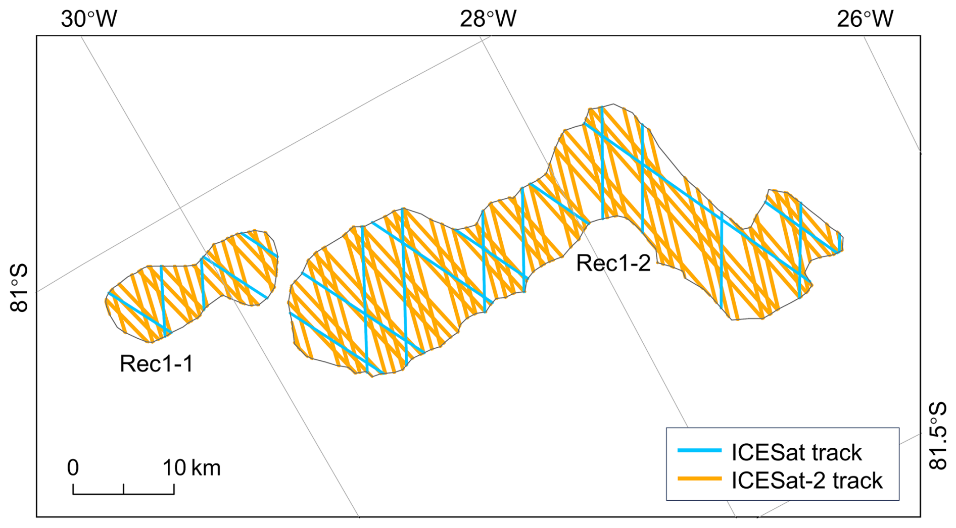
Figure 10 Comparison of ground track density between ICESat (blue tracks) and ICESat-2 (orange tracks) over the Rec1-1 and Rec1-2 subglacial lakes.

A typical example is Rec1, where sparse ICESat ground tracks and weak elevation signals at lake margins led to subjective delineations, with both one-lake and two-lake interpretations coexisting in previous studies (Smith et al., 2009; Fricker et al., 2014). With ICESat-2's higher track density (a comparison of ICESat and ICESat-2 track densities is shown in Fig. 10), we identify two subregions exhibiting opposite elevation change trends in multiple observation periods, indicating asynchronous filling-draining behavior. When these new outlines are retrospectively applied to ICESat data, asynchronous variations remain evident, confirming that Rec1 comprises two distinct lakes. To further investigate the hydrological connectivity between these two distinct lakes, we conduct quantitative analysis of lake volume changes during the ICESat-2 period (Fig. 11). This reveals that most water from Rec1-2 is preferentially delivered to Rec1-1 (with relatively consistent outflow and inflow volumes between them), while RecN1 shows only minor volume changes. However, the Shreve hydropotential model predicts water flow from Rec1-2 downstream along the primary hydrological network toward RecN1, excluding Rec1-1 from this pathway (Fig. 9a). This discrepancy may stem from errors in the surface and bed topography DEMs used for the hydropotential field, as small surface changes or moderate bed alterations can significantly redirect drainage pathways (Wright et al., 2008; Willis et al., 2016). Thus, integrating observations with model predictions is essential for assessing subglacial hydrological connectivity. Moreover, although Fricker et al. (2014) treated Rec1 as a single lake, RES data identified a subglacial channel in the Shackleton branch, implying dual drainage pathways: a dominant near-side route toward Rec1-1 (possibly along the Shackleton branch to the Slessor Glacier region) and a secondary path toward RecN1. By dividing Rec1 into two parts and analyzing interactions among Rec1-1, Rec1-2, and RecN1, this study provides further evidence supporting that inference.

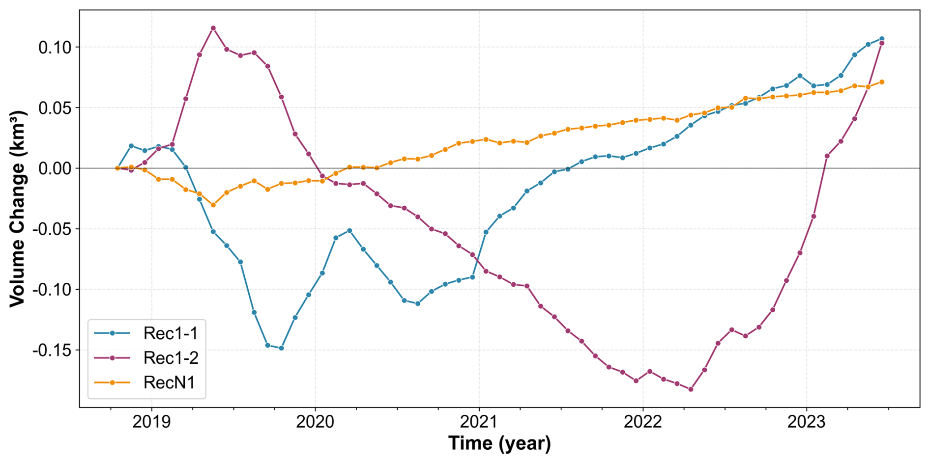
Figure 11 Volume changes of three subglacial lakes (Rec1-1, Rec1-2, and RecN1) during the ICESat-2 period (2018–2023). The solid lines represent the volume changes calculated from ICESat-2 elevation measurements, with data points marked by filled circles.

Subglacial drainage can exert substantial influence on basal melting of ice shelves, localized acceleration of ice flow, and thinning of the ice column (Gourmelen et al., 2025), yet current projections of Antarctic ice mass loss have not systematically incorporated the effects of subglacial drainage (Wilson et al., 2025). Moreover, model simulations suggest that the timing and magnitude of retreat in the East Antarctic RIS region may constitute a substantial fraction of the continent's future contribution to global sea level rise (Golledge et al., 2017). Accordingly, updating and continuous monitoring of active lakes in the RIS, with particular attention to the structure of interconnected subglacial networks and their drainage behaviour, will improve mass balance estimates, provide better constraints for coupled ice-flow–hydrology models, and reduce uncertainties in projections of East Antarctica’s future dynamics and sea level contribution.

5.2 Volume change uncertainty

Based on the 20-year observations in this study and combined with the elevation change time series shown in Figs. 5–7, it is evident that the lakes along the primary drainage networks have experienced multiple filling-draining events. Particularly between 2019 and 2023, all lakes completed 1–2 drainage events, implying a filling–draining cycle period of approximately 2–4 years for lakes in the primary drainage networks. We estimated the ratio of altimetry-derived volume change to the true volume change ($\mathrm{\Delta }{V}_{\mathrm{est}}/\mathrm{\Delta }{V}_{\mathrm{true}}$) for a filling-draining cycle of 3 years. For lakes in the main hydrological network, the ratio ranges from 0.53 to 0.93, with a mean value of 0.76. These results reveal underestimation of the true volume changes, highlighting a limitation that the satellite altimetry cannot fully capture the absolute magnitude of subglacial water exchange. Nevertheless, the altimetry data still successfully detect the occurrence of major filling-draining events, as demonstrated by the clustered filling-draining patterns among lakes along the primary hydrological network (Fig. 9b–c) and the fact that numerous lakes have experienced multiple filling-draining cycles over the 21-year observation period (Figs. 5–7). Moreover, the filling–draining periods differ among lakes and may also vary between successive events at an individual lake. Consequently, this variability makes it difficult to define a single, accurate period for lakes, thereby introducing errors in quantifying the bias caused by viscous ice flow. Future work should use new estimation methods that include ice flow physics to reduce the discrepancies introduced by the viscous transmission of basal volume changes to the surface (Stubblefield et al., 2021).

5.3 Cyclical variations in water volume and potential mechanisms

Examining the spatial patterns in more detail (as shown in Fig. 9c), observations indicate that during and after Period III, the system predominantly exhibits a pattern of upstream filling and downstream draining, which suggests that water continues to migrate downstream. The main difference after Period III lies in the amplitude of water volume changes, with both draining and filling amplitudes decreasing, and individual fluctuations generally smaller than those during Period III. Such variations in water volume are not unique to this period. Throughout the ICESat-2 observation period (Fig. 9c), water volume exhibits noticeable fluctuations: it is relatively high in the first half of 2019, declines over the following two years, rises again in the latter half of 2021, and then decreases once more. These observed water volume changes may result from variations in subglacial meltwater recharge. Given that subglacial water primarily originates from basal melting (Fricker et al., 2016), meltwater source may decline following periods of intensified drainage, and it may take time for water to accumulate before larger fluctuations in water volume occur again. In addition, fluctuations in water volume may be related to the evolution of subglacial drainage channels. As shown in Fig. 9c, a large water volume fluctuation is observed in the first half of 2019. Model simulations (Dow et al., 2016, 2018) suggest that periods of intensified drainage promote channel expansion, allowing water to be routed more efficiently through the system and accumulating meltwater to be drained rapidly. Over the following approximately two years (2020, 2021), meltwater recharge to the system decreases substantially, accompanied by a corresponding reduction in drainage volume. When recharge remains consistently low and available water decreases, the channels gradually contract or even close (Dow et al., 2016, 2018), reducing overall drainage efficiency. Over time, the lake accumulates additional meltwater until channels redevelop sufficiently to produce larger amplitude fluctuations in drainage volume, as observed in the latter half of 2022 (Period III). As channels mature, they evacuate meltwater rapidly, so that when meltwater source later declines, there is less stored water and subsequent fluctuations in volume are smaller, consistent with observations after Period III. The cyclical variation in water volume within the RIS may be primarily driven by the interaction between regional meltwater recharge and the evolving subglacial drainage channels, as suggested by both observational and modeling results; however, higher resolution observations and further model verification are still required to confirm this behavior.

5.4 Cascading dynamics of active subglacial lakes

Based on Fig. 9c, it is found that the major, periodic filling-drainage events of the lakes located along the primary drainage pathway are centered on Period III. We examine the filling-to-draining transition points of these lakes from early 2021 to mid-2023 to determine the drainage onset time for each lake, as shown in Fig. S6. This analysis reveals that lakes from upstream to downstream exhibit an almost sequential drainage pattern, forming a relatively complete subglacial hydrological system response event. Despite the fact that viscous relaxation of the ice may cause the surface elevation extrema observed by altimetry (the apparent highstand and lowstand times) to precede the true extrema of the subglacial water volume, the lakes involved in the cascading drainage event exhibit relatively short filling–draining cycle period, meaning that the resulting time lag is minimal and viscous relaxation is unlikely to alter the inferred hydrological connectivity or the sequence of drainage between lakes (Stubblefield et al., 2021). Therefore, the time offset is neglected in this study, and the altimetry-derived timing of surface extrema is used in the subsequent cascading drainage analysis.

The schematic diagram of the cascading drainage pattern along the primary drainage pathways of RIS is shown in Fig. 12. The drainage process initiates at the most upstream lake, RecN10, which begins draining in June 2019. The drainage of RecN10 triggers synchronous water recharge in the downstream lakes Rec9 and RecN9. After nearly two years of almost continuous filling, these two lakes reach their drainage thresholds in May and August 2021, respectively, and begin draining successively. Subsequently, lakes RecN6 and Rec6-2, located approximately 200 km downstream of lake RecN9, begin draining in November of the same year, with this propagation process taking only about 3 months. This may be attributed to the descending bed topography in this section, which accelerates the water transport rate. Further downstream, lake Rec4 begins draining in March 2022, however, its downstream lake RecN4 begins draining approximately one month earlier. This reverse-sequence drainage phenomenon may stem from the area differences between the two lakes: Rec4 has an area exceeding 200 km², more than three times that of lake RecN4. Large-area lakes may require longer water recharge time to reach the drainage threshold, suggesting that lake geometric characteristics play an important role in controlling cascading drainage timing. The section from RecN4 to RecN2 spans approximately 130 km, where the bed elevation shows an increase, yet the cascading drainage effect still completes transmission within about six months. This indicates that although topographic highs may slow the propagation speed, they do not completely block subglacial hydrological connectivity. Subsequently, the propagation reaches the terminal region, where the two lakes RecN2 and Rec1-2 remain recharging throughout the observation period without reaching the drainage threshold. This typical cascading drainage pattern indicates that the subglacial hydrological system beneath the RIS is highly connected, capable of transmitting drainage perturbations over long distances despite modest topographic variability. Such phenomena could potentially affect basal sliding and thus influence ice mass loss.

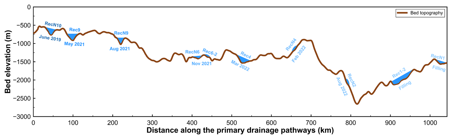
Figure 12 Cascading drainage pattern along the primary drainage pathway of the RIS. The bed topography (brown line, data from BedMachine V3; Morlighem, 2022) and subglacial lake positions (blue filled areas) are shown along the drainage network from upstream (left) to downstream (right). Color gradient denotes the timing of initial drainage events. Terminal lakes Rec1-2 and RecN1 did not drain during the observation period (marked “Filling”). The origin of the x axis corresponds to the red star in Fig. 9a.

The drainage onset time of other lakes distributed in the upstream area of RIS, including RecN12 and RecN14, is around June 2019 and continues until the end of the observation period. This drainage pattern, characterized by spatially dispersed lake locations but temporally synchronized elevation changes, suggests that there may exist a common catchment area or meltwater supply system in the upstream region, with these lakes connected to a common source region through the subglacial river network system. The sustained drainage cycle lasting four years indicates that this catchment area may possess substantial water storage capacity, capable of maintaining long-term stable meltwater supply.

Although Fricker et al. (2014) reported a cascading drainage event beneath the RIS, our observed cascade demonstrates significant expansions: the spatial distance has widened from the previous 800 km to roughly 1000 km, while the number of participating lakes has more than doubled from the original four to ten (RecN10, Rec9, RecN9, RecN6, Rec6-2, Rec4, RecN4, RecN2, Rec1-2, and RecN1). This increased transmission distance and lake involvement indicate a more extensive and highly interconnected subglacial lake network, which may reflect improved detection capabilities by ICESat-2 and/or genuine temporal changes in subglacial connectivity. In addition, elevation changes observed in lower trough lakes during IceBridge indicate that hydrological activity still exists during the interval between the two large-scale cascading events, suggesting that RIS may not have stopped subglacial hydrological activity during 2003–2023.

Based on this expanded network, we further analyze the characteristics and possible mechanisms of its water volume changes. We find that the magnitudes of both individual and cumulative water volume changes during the ICESat-2 observation period cascading event are smaller than those observed during the ICESat period event (Fig. 9). This pattern may reflect several interconnected processes. For example, over time the RIS region may have developed a more mature drainage system: enhanced connectivity and increasingly stabilized channels facilitate downstream transport rather than temporary storage within a single lake, thereby reducing the amplitude of lake volume fluctuations. At the same time, the number of lakes involved in recent years cascade has increased substantially, which may have distributed the available water across a larger set of basins and further diminished the volume change observed at individual lakes. Finally, it is also possible that upstream water supply has decreased, reducing the total amount of water available for filling and draining. These mechanisms may operate individually or in combination, collectively contributing to the smaller water volume amplitudes observed in recent years. Beyond the changes in spatial extent and water volume, on the temporal scale, the two cascading events show similar characteristics. In the event recorded by Fricker et al. (2014), drainage propagates from lake Rec9 before 2003 to lake Rec1 in 2008; in the event observed in this study, it propagates from lake RecN10 in June 2019 to lakes RecN2 and Rec1-2 in June 2023 (still filling). Both events show that water propagation along the main drainage network from upstream to downstream in the RIS system requires at least 4–5 years. More importantly, although the two drainage events are separated by more than a decade, the propagation time and spatial patterns are relatively consistent, which indicates that the Recovery system has stable and persistent drainage channels.

Compared with the Siple Coast, the RIS demonstrates substantially greater hydrological persistence and system scale connectivity. The Siple Coast subglacial network is readily reorganized by modest, local ice-thickness perturbations, so that channels and lakes frequently change configuration (Anandakrishnan and Alley, 1997; Carter et al., 2013). By contrast, the RIS is characterized by a relatively stable and spatially extensive drainage structure. The bedrock elevation gradient in the Recovery region is significantly greater than the surface elevation gradient, rendering the system less sensitive to short-term surface ice thickness perturbations (Fricker et al., 2014). Modelling by Dow et al. (2018) shows that drainage channels downstream of Recovery can persist for several years following lake drainage events, with the overall hydrological behaviour governed by a regional drainage network spanning hundreds of kilometres. Our observations align with this: in the Recovery region, subglacial water can be transported downstream over distances of approximately 1000 km, with individual events lasting at least 4–5 years. This long-distance and long-duration transport capability indicates that the high connectivity in Recovery not only prolong channel persistence but also expand the spatial propagation scale of drainage events, thereby supporting sustained subglacial water transport on a continental scale.

The cascading drainage pattern observed along the main RIS pathway shows certain similarities with observations from Jutulstraumen Glacier (JG) (Neckel et al., 2021). The topographic configuration at JG is characterized by subglacial water generated in a large upstream catchment area that must converge through a relatively narrow constriction zone starting from the onset of ice streaming (Neckel et al., 2021). This configuration is relatively consistent with that of the RIS: the upstream region contains spatially dispersed lakes, while the most active downstream drainage converges into a relatively narrow bedrock trough. This topographic characteristic, transitioning from a broad upstream catchment to a narrow downstream channel, is likely a key geomorphological factor promoting the development of an efficient channelized drainage system. Despite the similarities in drainage pattern and topographic setting, the two systems differ in their spatiotemporal scales. The cascading drainage event at JG propagates along approximately 175 km of flow path over about one year (Neckel et al., 2021). In contrast, the RIS drainage event we observe exceeds JG in both spatial and temporal scales: the drainage propagation distance reaches roughly 1000 km, and the entire event lasts at least 4 years. This significant scale expansion likely reflects the more extensive catchment system and substantially larger drainage network of the RIS.

6 Conclusions

The recent activity of nine reported subglacial lakes in the RIS region is investigated based on ICESat-2 satellite altimetry data. It is found that five reported lakes show low levels of activity during the ICESat-2 period. Four other lakes have shown changes in their activity range compared to previous observations. The updated outlines of these lakes are given in this study. Moreover, 14 new active lakes (named RecN1–N14) are discovered. This extended observational record demonstrates that the drainage regime in RIS is characterized by long-term, sustained water transport. The long-term elevation changes of these lakes from 2003 to 2023 are established by integrating altimetry data from ICESat, Operation IceBridge's ATM measurements, and ICESat-2. Among the reported lakes, lakes Rec1-1, Rec1-2, Rec2, Rec4, Rec6-1, and Rec6-2 remain active (with elevation changes over 0.5 m) throughout the 20-year time series. Most of the newly detected lakes are identified mainly due to their activity during the Operation IceBridge and ICESat-2 periods, particularly lakes RecN4, RecN9, and RecN11, which exhibit high levels of activity (over 2 m). Elevation change analysis at crossovers on four representative lakes reveals that the lakes' central regions exhibit greater variation than the surrounding areas, with a maximum difference of up to 4 m. Our results also reveal that Rec1 consists of two distinct lakes (Rec1-1 and Rec1-2), exhibiting different drainage and accumulation characteristics. Based on their volume transfer patterns, we analyze the hydrological connectivity between them, which lends additional support to the earlier hypothesis that the RIS hosts two subglacial drainage outflows. Additionally, quantitative analysis of volume changes for 11 lakes distributed along primary hydrological pathways reveals systematic volume fluctuations and temporal synchronization of volume changes, suggesting water exchange relationships among these lakes. Through turning point identification in the elevation time series, we detect a cascading drainage event involving 10 lakes along primary drainage pathways and spanning over 1000 km, with sequential drainage from upstream to downstream, demonstrating a highly connected subglacial hydrological system in this region during our observation period. Future studies could introduce hydrological models to explore the response mechanisms of ice sheet internal hydrological systems and their impact on glacier dynamics, providing more comprehensive scientific evidence for assessing Antarctic ice sheet stability and its influence on global sea level changes.