Results of the second Ice Shelf–Ocean Model Intercomparison Project (ISOMIP+)

Ocean-driven basal melting of Antarctic ice shelves plays an important role in the mass loss of the Antarctic Ice Sheet. Ice shelf cavity-resolving ocean models are a valuable tool for understanding ice shelf-ocean interactions and for simulating projections of ice shelf and ocean states under future climate. Designed to assess the current state of ice shelf–ocean modelling, the second Ice Shelf–Ocean Model Intercomparison Project, ISOMIP+, consists of 12 ocean model configurations submitted with a common, idealised experimental setup. Here, we focus on the experiments Ocean0–2 (Asay-Davis et al., 2016), which are ocean models with idealised, static ice shelf geometries, but where the ocean reaches a balance with prescribed far-field ocean conditions. Different thermal transfer coefficient values (ranging from 0.011 to 0.2) are used for each model in the melting parameterisation to achieve a common, tuned melt rate since the models cover a range of types of vertical coordinates, ice–ocean boundary layer treatments, and numerical schemes. These model differences lead to spread in the resultant ocean properties, circulation, boundary-layer structure and spatial distribution of melting. We also highlight similarities between models, such as a shared linear relationship across most models between melt rate and overturning and barotropic streamfunctions during the spin-up and spin-down, demonstrating a robust relationship between melt and circulation across models and forcing conditions. The ISOMIP+ results provide a systematic comparison of ice shelf cavity-capable ocean models. However, we also demonstrate the need for realistic ice shelf–ocean model intercomparison projects (some already underway) to assess model biases and inter-model variation against sparse observations. Further research is needed to understand the differences between models and further improve our modelled representations of the ice–ocean boundary layer and ice shelf cavity circulation.

1 Introduction

The projection of ice sheet behaviour is paramount for understanding, mitigating, and adapting to the impacts of climate change on global sea level. The Antarctic Ice Sheet, which contains most of the world's frozen freshwater, is a key driver of sea level rise over decadal and longer timescales (IPCC, 2021) and also has strong interactions with the Southern Ocean and global thermohaline circulation (e.g. Fogwill et al., 2015; Bronselaer et al., 2018; Golledge et al., 2019; Li et al., 2023) and therefore global climate. With global temperatures increasing, the sea level rise indirectly caused by the melting of ice shelves poses significant risks to coastal communities, infrastructure and ecosystems worldwide (Bronselaer et al., 2018; Sadai et al., 2022; Galton-Fenzi et al., 2025a). Consequently, accurate projections of ice sheet behaviour, particularly in response to the ocean-driven basal melting of ice shelves, are crucial for informing climate policy, coastal planning, and disaster preparedness (Hinkel et al., 2019; Durand et al., 2022).

To address this challenge, numerical models have been developed to simulate the interactions between ice shelves and the ocean (e.g. Williams et al., 1998; Dinniman et al., 2016; Asay-Davis et al., 2017; Rosevear et al., 2025). These models are indispensable for understanding how ocean processes drive ice shelf melting and for projecting how ice sheets will respond to warming oceanic conditions (e.g. Holland et al., 2008; Gwyther et al., 2016; Seroussi et al., 2020; Naughten et al., 2023; Kusahara et al., 2023). However, there are still uncertainties in these simulations associated with model differences (Naughten et al., 2018b), compounded by uncertainties in ice sheet model projections (IPCC, 2021; Seroussi et al., 2020). The first iteration of the Ice Shelf–Ocean Model Intercomparison Project (ISOMIP) was conceived in the early 2000s through the Forum for Research into Ice Shelf Processes (FRISP) (https://scar.org/science/physical/frisp, last access: 1 April 2026), in response to the need for improving the accuracy and reliability of simulations by providing a standardised framework for their comparison and enhancement (Holland et al., 2003; Hunter, 2006). Through a common set of protocols and test cases for model evaluation, different models were systematically compared using highly idealised geometries and simplified physical conditions based on the original “Grosfeld” cavity (Grosfeld et al., 1997). This collaborative endeavour facilitated the identification of strengths and weaknesses of various modelling approaches and fostered model development. Although a formal ISOMIP comparison was not published, several studies used the protocol to demonstrate the importance of simulation of the sub-ice shelf circulation and associated numerical modelling choices for the computed melt rates in individual models (e.g. Hunter, 2006; Losch, 2008; Holland et al., 2008; Galton-Fenzi, 2009; Little et al., 2009; Gwyther et al., 2015, 2016; Mathiot et al., 2017). Many of these ISOMIP studies also show good model agreement with the Grosfeld et al. (1997) benchmark, providing confidence in the numerics and physics of ice shelf–ocean models, at least in an idealised setting.

Community engagement in ice sheet–ocean modelling was revitalised through the Climate and Cryosphere (CliC) project of the World Climate Research Programme (WCRP), resulting in the establishment of the Marine Ice Sheet–Ocean Model Intercomparison Project in 2014 (MISOMIP;  Holland and Holland, 2015). MISOMIP sought to develop a suite of coupled glacier–ocean model benchmark tests using more complex ice and bed topography but still idealised model configurations. An ice sheet-only experiment (MISMIP+) was already under development, based on previous standalone marine ice sheet model intercomparisons (Pattyn et al., 2012, 2013). MISOMIP developed two complementary tests, an ocean-only set of simulations (ISOMIP+) and coupled ice sheet and ocean simulations (MISOMIP1), that together comprised the next-generation framework for idealised ice sheet-ocean model intercomparison (Asay-Davis et al., 2016). Building complexity on the idealised ISOMIP (Hunter, 2006) and MISMIP (Pattyn et al., 2012, 2013) frameworks, a common, high-resolution domain was used for MISMIP+, ISOMIP+ and MISOMIP1. The domain used in these experiments was designed to be representative of small-sized, laterally confined ice shelves that experience buttressing, such as Pine Island Glacier Ice Shelf. These ice shelves are thought to be particularly vulnerable to retreat and are potentially major contributors to sea level rise because of the large volumes of grounded ice contained in the regions they buttress (Rignot et al., 2014; Favier et al., 2014; Christianson et al., 2016; Reed et al., 2024). The ISOMIP+ protocol specifies experiments testing the response to both warm and cold ice shelf cavity conditions and the transition between them. ISOMIP+ also builds on the first generation of ISOMIP by using a higher spatial resolution (from ∼ 3–9 km horizontal resolution and at least 10 vertical layers to ∼2 km and 36 vertical layers Hunter, 2006; Asay-Davis et al., 2016), a velocity-dependent basal melt parameterisation (Holland and Jenkins, 1999; Jenkins et al., 2010), and a more complex bottom topography and ice draft that introduces aspects of reality, but is still constrained by the topography requirements for the ice sheet models in the parallel MISMIP+ and MISOMIP1 experiments. The added complexity of ISOMIP+ compared with ISOMIP likely amplifies the effect of model choices and therefore increases model spread, but also exposes what model choices may be important in realistic ice shelf–ocean simulations.

The ISOMIP+ protocol (Asay-Davis et al., 2016) has been used extensively for model comparison and development. Gwyther et al. (2020) use three ISOMIP+ models to assess the sensitivity of melt rate to specific model choices in the melt parameterisation; specifically, the distance over which a far-field temperature is sampled, and the distance over which freshwater or melt fluxes are distributed. Scott et al. (2023) and Zhou and Hattermann (2020) use the framework to verify and assess new unstructured grid ice shelf cavity ocean models. Additionally, Scott et al. (2023) explore the sensitivity of melt rate to vertical resolution and find that melt rates converge at high vertical resolution, whilst Zhou and Hattermann (2020) quantify pressure gradient errors. Stern et al. (2017, 2019) use a modified ISOMIP+ setup to test a Lagrangian iceberg model. Yung et al. (2025) use two ISOMIP+ ocean models to evaluate a basal melt parameterisation incorporating the unresolved feedback effect of stratification due to buoyant meltwater suppressing boundary layer turbulence and therefore melt rates. Buissou et al. (2022) use some ISOMIP+ simulations to train and assess melt parameterisations based on neural networks, and Vaňková et al. (2025) explore relationships between melt and subglacial discharge in an ISOMIP+ model. Many of these studies, as well as earlier ISOMIP studies, explore sensitivities to resolution and melt parameterisation choices – reconciling parameterised melt with real observed ice shelf melt and cavity regimes remains a challenge for the community.

The related MISOMIP1 protocol has also been used for model development: Zhao et al. (2022) explore sub-ice shelf melt oscillations and the relationship with ocean circulation with the MISOMIP1 setup, whilst Favier et al. (2019) use the MISOMIP1 setup to assess basal melt parameterisations for stand-alone ice sheet models. Zhou et al. (2024) use two ocean models with MISOMIP1 configurations to assess an accelerated forcing approach to coupled ice sheet–ocean modelling. Smith et al. (2021) develop the ice shelf–ocean coupling framework used in the UKESM1 climate model using the MISOMIP1 test case and assess the impact of grid resolution on coupling feedbacks. Richter et al. (2025) use the MISOMIP1 setup to develop and verify a coupled ice sheet–ocean model framework. These studies demonstrate the benefit of common, idealised protocols in facilitating advances in ice shelf–ocean models.

Model developments in idealised experiments can support and ultimately transition to realistic domains for future projections of Antarctic ice shelf melt (e.g. Timmermann and Hellmer, 2013; Naughten et al., 2018a; Siahaan et al., 2022; Jourdain et al., 2022; Kusahara et al., 2023; Mathiot and Jourdain, 2023; Naughten et al., 2023; Bett et al., 2024; De Rydt and Naughten, 2024) and guide melt parameterisations for simulations used in current and future Intergovernmental Panel on Climate Change (IPCC) reports (Jourdain et al., 2020, 2022; Burgard et al., 2022). Additionally, two realistic Antarctic ice sheet–ocean model intercomparison projects have been established since ISOMIP+, the Realistic Ice-shelf/ocean State Estimates (RISE;  Galton-Fenzi et al., 2025b) project focused on comparing and evaluating existing circum-Antarctic ice shelf–ocean simulations and the Marine Ice Sheet and Ocean Model Intercomparison Project – phase 2 (MISOMIP2;  De Rydt et al., 2024, the next iteration of the MISOMIP collaboration), focused on the ice sheet–ocean interactions in the Weddell and Amundsen Seas. Whilst realistic model intercomparisons facilitate validation with observations (where they exist) and future projections, they also have added complexity that makes untangling the consequences of model choices more difficult: therein lies the value of idealised models as a well-controlled verification and benchmarking tool, which will likely continue to be used in future model development as we seek to achieve model agreement with the real world.

Here, we report the results of ISOMIP+, consisting of contributions from 12 model configurations. These contributions, which include eight independent ocean models, demonstrate the increasing number of ocean models that can simulate ice shelf cavities (Dinniman et al., 2016) and the successful reach of the collaborative model intercomparison approach. After summarising the Asay-Davis et al. (2016) experimental protocol and detailing the model configurations, we present the modelled ocean properties, melt rates and drivers of melt (friction velocity and thermal driving, used in the basal melt parameterisation) and ocean cavity circulation. While we verify the internal consistency of the basal melting parameterisation and water mass conservation, we cannot validate the idealised simulations with observations, and no analytical solutions have been found. Instead, we present and compare the model results as a diagnostic benchmarking exercise, and aim to understand the causes of their similarities and differences where possible. We identify key aspects of model variability on which future work can focus as we progress towards improved ice shelf–ocean model fidelity.

2 Experimental design

The ISOMIP+ protocol, documented by Asay-Davis et al. (2016), consists of five different experiments using ocean models: a tuning experiment (Ocean0), two experiments with static ice shelves and a warming or cooling ocean boundary forcing (Ocean1 and Ocean2), and two experiments with a prescribed retreat and re-advance of the ice shelf grounding lines (Ocean3 and Ocean4). In this study, we do not describe the latter two experiments with dynamic ice shelves. Their results are provided in an analysis of a separate intercomparison for the MISOMIP1 two-way coupled ice sheet–ocean models (Hélène Seroussi and Nicolas Jourdain, personal communication, 2026). The ISOMIP+ experiments use common geometries (bed topography and the ice shelf draft), boundary and initial conditions, and mixing and melt parameterisations. In this section, we briefly summarise the protocol and refer the reader to Asay-Davis et al. (2016) for further details. This study focuses on the “common” (COM) experiments where models strictly follow the protocol and are tuned to achieve similar melt rates. Some participants also submitted “typical” (TYP) results for their models where parts of the model protocol were relaxed, described in Sect. 2.7.

2.1 Geometric setup

The ISOMIP+ bed topography and ice shelf draft (Fig. 1) are idealised geometric configurations that overlap with the MISMIP+ (Cornford et al., 2020; Asay-Davis et al., 2016) and MISOMIP1 domain. The domain has size 480 and 80 km in the x and y directions, respectively, though part of this domain (x<400 km) contains only grounded ice and is therefore not included in our figures. The x direction aligns with the direction of the ice flow, towards the calving front. This choice does not affect the ocean circulation, since the participating models use the f-plane approximation (referenced to 75° S latitude). The bed topography is the same as MISMIP+ and the ice shelf draft for Ocean0 and Ocean1 is a steady state ice shelf configuration computed with the BISICLES model (Cornford et al., 2013) with the MISMIP+ Ice1 parameters (Asay-Davis et al., 2016; Cornford et al., 2020), and computed similarly for Ocean2 with MISMIP+ Ice1r parameters. The BISICLES geometry includes a steep calving front located at x=640 km. The bed topography (also provided as an analytic expression;  Asay-Davis et al., 2016) and ice shelf draft were provided on a 1 km horizontal resolution grid. Participants then interpolated and smoothed the bed topography and ice shelf draft using different methods to achieve a horizontal grid resolution of 2 km (details are in Sect. 3; see Figs. S11, S12 in the Supplement). However, where interpolation results in an ice shelf thickness less than 100 m, the thickness is set to zero to represent a steep calving front, except where smoothing of the calving front was required for model stability. Models are configured with 36 vertical levels, spread over the 720 m maximum depth in different ways depending on the vertical coordinate used, resulting in varying vertical resolution beneath the ice shelf. All z-level models use a vertical grid size of 20 m with differing partial cell choices. In the Ocean0-2 experiments discussed in this paper, the ice shelf draft is fixed and does not change in time.

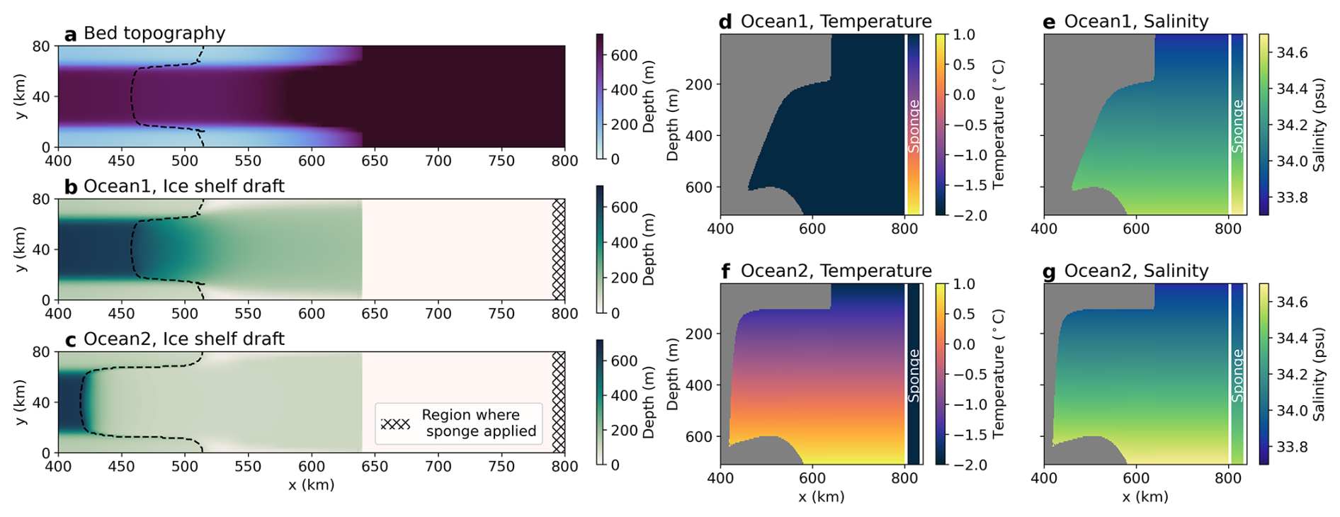
Figure 1 Experiment geometry and initial conditions, showing the bed topography (a), and ice shelf draft for the Ocean0 and Ocean1 (b) and Ocean2 (c) experiments, and cross sections at y=40 km of the temperature and salinity initial conditions for Ocean1 (“cold initial conditions”, d, e) and Ocean2 (“warm initial conditions” f, g). The sponge forcing applied at the positive x boundary is the opposite (cold/warm) of the initial conditions, therefore once models have been run to an equilibrium state, Ocean1 has “warm” conditions and Ocean2 “cold”. Ocean0 uses the warm initial conditions and warm sponge boundary.

2.2 Initial and boundary conditions

The initial conditions for the experiments are either a “warm” or “cold” profile (Fig. 1d–g). Potential temperature (referred to as temperature in the remainder of this manuscript) and practical salinity (noting that we use the PSS-78 salinity scale, so values do not have units) vary linearly with depth. For the cold profile (qualitatively representative of the Ross or Weddell Seas), the temperature is a constant −1.9 °C and salinity varies linearly between 33.8 at the surface (0 m depth) to 34.55 at the bottom (720 m). For the warm profile (qualitatively representative of the Amundsen and Bellingshausen Seas, with warm, salty Circumpolar Deep Water intrusions at depth, e.g., Dutrieux et al., 2014), the temperature and salinity varies from -1.9°C and 33.8 at the surface to +1 °C and 34.7 at the seafloor. By making use of the experiment's linear equation of state, the cold and warm profiles are designed to have the same density profile (Fig. 6 from Asay-Davis et al., 2016) to reduce convective instabilities. Having the same density profile also means that density variations are solely created by ice shelf meltwater, not by the boundary (Holland, 2017). However, the salinity stratification of the cold profile is stronger than the conditions observed in cold Antarctic ice shelf cavities (e.g. Orsi and Wiederwohl, 2009; Nicholls et al., 2004; Darelius et al., 2014). In all experiments, the ocean begins at rest.

The boundaries on all side walls use no-slip conditions whilst top and bottom boundaries employ a quadratic drag with drag coefficient C_D. Additionally, the temperature and salinity are forced using a restoring sponge at the “northern” x boundary. This sponge is applied over the entire ocean depth and y direction, and linearly increases in restoring strength from no restoring at x=790 km to full restoring at x=800 km, with a restoring timescale of 0.1 d (i.e. 2.4 h) towards either the warm or cold profile. To avoid sea level rise over the course of the simulation, sea level may also be restored if melting is implemented as a volume flux using surface mass fluxes in the sponge restoring region; otherwise, there are no open ocean surface fluxes (unless specified in Sect. 3, see also the Meltwater addition column of Table 2).

2.3 Equation of state

The experiment protocol prescribes a linear equation of state given by

$$\begin{array}{}\text{(1)}& \mathit{\rho }={\mathit{\rho }}_{\mathrm{ref}}\left[\mathrm{1}-\mathit{\alpha }(T-T_{\mathrm{ref}})+\mathit{\beta }(S-S_{\mathrm{ref}})\right],\end{array}$$

where the reference density, temperature and salinity are ρ_ref, T_ref and S_ref, and the thermal expansion and haline contraction coefficients are α and β. Numerical values are presented in Table 1.

Table 1 Parameters for the ISOMIP+ common experiments, reproduced from Asay-Davis et al. (2016).

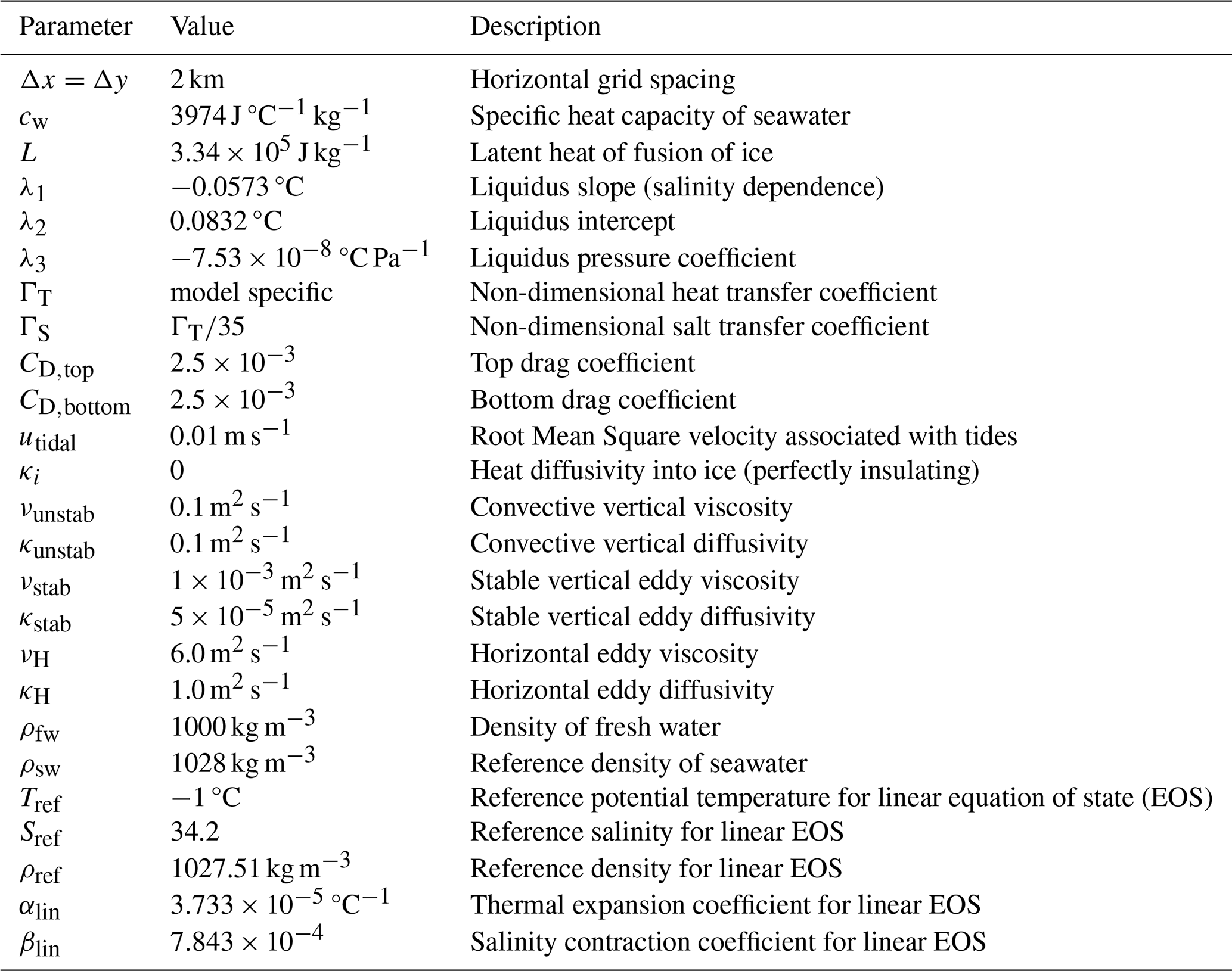
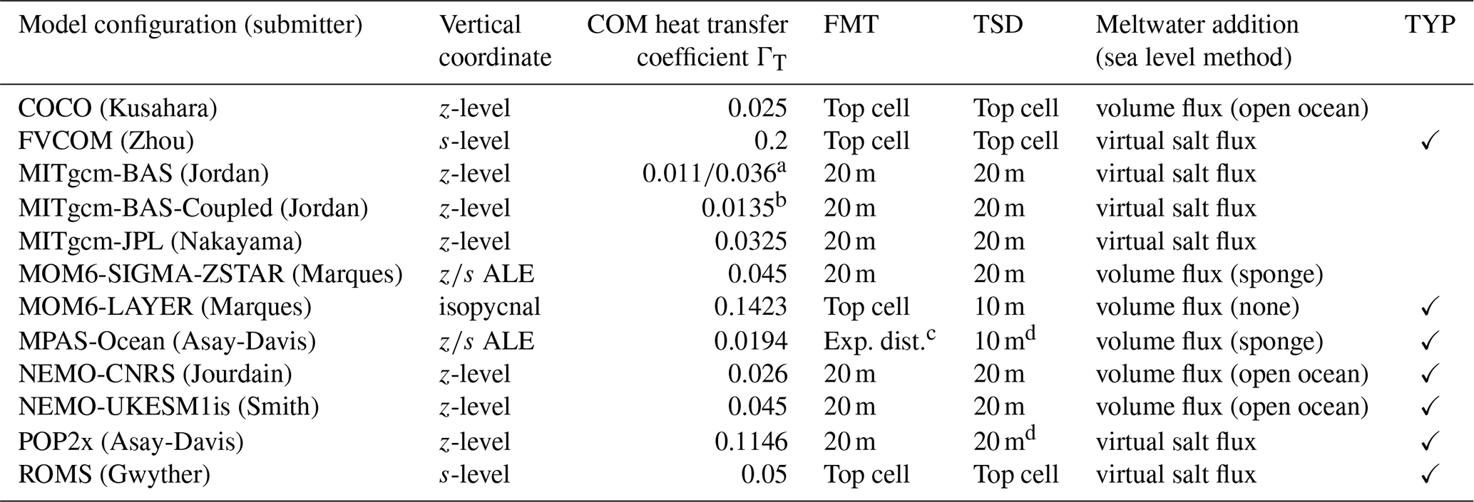
Table 2 Summary of the model configuration submissions for the ISOMIP+ Ocean0, Ocean1 and Ocean2 experiments. We list the vertical coordinate (z-level, sigma/terrain-following (s-level), isopycnal, and $z/s$ ALE for Arbitrary Eulerian-Lagrangian coordinates. In the latter, z coordinates in the open ocean transition into an ice shelf draft-following target coordinate in the ice shelf cavity; see Stern et al. (2019) and Comeau et al. (2022) for further details), heat transfer coefficient for COM experiments, the flux mixing thickness (FMT, vertical distance over which meltwater was spread), tracer sampling distance (TSD, for the melt parameterisation), meltwater addition method and whether TYP Ocean1 and Ocean2 experiments were also submitted. The method of meltwater addition is either a virtual salt flux or volume flux. In the case of a volume flux, we also specify whether the sea level is constrained to be constant via an adjustment applied to the entire open ocean, applied to just the sponge boundary, or not constrained (“none”). COM salt transfer coefficients were fixed according to ${\mathrm{\Gamma }}_{\mathrm{S}}={\mathrm{\Gamma }}_{\mathrm{T}}/\mathrm{35}$.

^a Derived transfer coefficient for Ocean1 simulation is 0.011 and 0.036 for Ocean2, see Sect. 3.3 for more details. ^b Using derived transfer coefficient rather than reported value (Sect. 3.3). ^c See Sect. 3.5. ^d Velocity sampled only in top cell.

2.4 Melt parameterisation

Ice shelf basal melt rates are calculated using the three-equation parameterisation (Hellmer and Olbers, 1989; Holland and Jenkins, 1999) with a linear dependence of the freezing temperature on pressure and salinity and constant transfer coefficients (Jenkins et al., 2010):

$$\begin{array}{}\text{(2)}& {\displaystyle }{T}_{z_{\mathrm{d}}}={\mathit{\lambda }}_{\mathrm{1}}{S}_{z_{\mathrm{d}}}+{\mathit{\lambda }}_{\mathrm{2}}+{\mathit{\lambda }}_{\mathrm{3}}{p}_{z_{\mathrm{d}}}\text{(3)}& {\displaystyle }{\mathit{\rho }}_{\mathrm{fw}}{m}_{\mathrm{w}}L=-{\mathit{\rho }}_{\mathrm{sw}}{c}_{\mathrm{w}}{u}_{*}{\mathrm{\Gamma }}_{\mathrm{T}}(T_{z_{\mathrm{d}}}-T_{\mathrm{w}})\text{(4)}& {\displaystyle }{\mathit{\rho }}_{\mathrm{fw}}{m}_{\mathrm{w}}{S}_{z_{\mathrm{d}}}=-{\mathit{\rho }}_{\mathrm{sw}}{u}_{*}{\mathrm{\Gamma }}_{\mathrm{S}}(S_{z_{\mathrm{d}}}-S_{\mathrm{w}})\text{(5)}& {\displaystyle }{u}_{*}^{\mathrm{2}}=C_{\mathrm{D}}\left(u_{\mathrm{w}}^{\mathrm{2}}+u_{\mathrm{tidal}}^{\mathrm{2}}\right).\end{array}$$

All parameters are described in Table 1. Here, the liquidus slope is λ₁, intercept λ₂ and pressure coefficient λ₃. The melt rate m_w is expressed as a freshwater flow rate (m s⁻¹), which is solved by the equations along with the temperature and salinity at the ice–ocean interface $T_{z_{\mathrm{d}}}$ and $S_{z_{\mathrm{d}}}$. The temperature T_w, salinity S_w and velocity u_w represent the ocean properties outside of the turbulent ice-ocean boundary layer and can be determined by models in different ways, but are generally taken as the surface mixed layer properties or properties averaged over a constant distance from the ice. Salt and freshwater densities are ρ_sw and ρ_fw. The latent heat of fusion is L and the specific heat capacity of water is c_w. The drag coefficient C_D for determining the friction velocity is the same as the dynamic drag boundary condition at the top and bottom boundaries.

Here, the prescribed tidal velocity u_tidal is used to account for the additional ocean motion (ostensibly due to tides) in the friction velocity (u_*). Without this prescribed velocity, no melt would occur when the ocean is at rest, even when heat is available for melting, contradicting our expectations from both theory and observations. It is worth noting that there are more complex and accurate methods to include the effect of tidal motion (Jourdain et al., 2019). The transfer coefficients Γ_T and ${\mathrm{\Gamma }}_{\mathrm{S}}={\mathrm{\Gamma }}_{\mathrm{T}}/\mathrm{35}$ are tuned constants (see Sect. 2.6). Using constant transfer coefficients is an approximation that does not hold in the real world, and models may use variable transfer coefficients (e.g. Holland and Jenkins, 1999). Furthermore, the ice is considered to be perfectly insulating without any conductive heat flux at the ice–ocean interface. For a review on melt parameterisations in ice shelf–ocean models, see Malyarenko et al. (2020) and Rosevear et al. (2025).

Gwyther et al. (2020) demonstrate with the ISOMIP+ setup that melt rates are impacted by both the distance across which the ocean properties subscript w are sampled (tracer sampling distance, TSD) and the distance across which the meltwater is distributed (flux mixing thickness, FMT). The ISOMIP+ model contributions vary in their sampling and distribution methods (Table 2); these are described further in Sect. 3. Additionally, models vary in their addition of freshwater, either as a volume or virtual salt flux (Table 2).

2.5 Mixing parameterisation

The mixing of momentum and tracers in vertical and horizontal directions is parameterised using a Laplacian (harmonic) operator with constant coefficients (values are prescribed in Table 1). Vertical (or more precisely, between model layers) diffusivity is κ_stab, except when there is locally unstable stratification, where it increases to account for convective instability (to κ_unstab) or using a model-dependent convective adjustment scheme described in Sect. 3. Similarly, the vertical viscosity ν_stab in the interior also increases with unstable local stratification to ν_unstab. Horizontal diffusivity and viscosity are κ_H and ν_H, respectively, though numerical mixing may also be significant. Mixing also occurs implicitly via the distribution of meltwater: typically, z-coordinate models use a Losch (2008)-style scheme where meltwater is distributed evenly over a fixed distance from the ice. This distance is usually the z-coordinate thickness, which usually covers multiple grid cells if partial cells are used. Other models may distribute meltwater only in the uppermost cell, thereby removing the implicit mixing due to meltwater distribution (details in Sect. 3).

2.6 Experiments Ocean0, Ocean1 and Ocean2

The Ocean0 tuning experiment uses the warm initial conditions and warm northern boundary sponge forcing with the ice draft of Fig. 1b. This allows a quasi-equilibrium, warm-shelf melt rate and circulation to be attained quickly. For the COM experiments, participants were requested to modify Γ_T (and consequently ${\mathrm{\Gamma }}_{\mathrm{S}}={\mathrm{\Gamma }}_{\mathrm{T}}/\mathrm{35}$ also varies) to achieve a target area-averaged melt rate at depth ($z<-\mathrm{300}$ m) of 30±2 m yr⁻¹. This tuning involved running multiple Ocean0 configurations to sample various Γ_T until the target melt rate was achieved, with larger Γ_T producing more melt via Eqs. (3)–(4). The Ocean0 simulations use these optimal transfer coefficients and were run for 1 year, or longer if quasi-equilibrium was not achieved within 6 months.

Ocean1 and Ocean2 use the same optimally tuned transfer coefficients as Ocean0 but with different restoring forcing, initial conditions and/or ice draft. Ocean1 begins with cold initial conditions but a warm restoring boundary (Fig. 1d) and same ice draft as Ocean0 (Fig. 1b), whereas Ocean2 begins with warm initial conditions and a cold restoring boundary (Fig. 1f) and a different ice draft (Fig. 1c), consisting of a steeper ice base slope over a narrower x-axis extent compared to Ocean1. Both experiments are run for 20 years to investigate the timescales and ocean states during the transition between warm and cold states of an ice shelf cavity.

2.7 Typical experiments

In their typical usage (for both realistic and idealised simulations), ice shelf–ocean model configurations generally differ from the prescribed ISOMIP+ protocol. For example, they may employ different mixing schemes, horizontal resolutions, or ice shelf melt parameterisations (e.g. Holland and Jenkins, 1999). The typical “TYP” simulations submitted by participants use the same geometry and boundary conditions as the Ocean0-2 COM experiments but with other parameters, resolutions, or physics schemes configured per participant choices for more conventional use, with these settings often taken from previous simulations. Since ice shelf melt parameterisations may have been modified, most TYP experiments do not use a tuned transfer coefficient to achieve the COM Ocean0 target melt rate. The TYP experiments provide an additional measure of variability between models, which are compared in Sect. 4.5. Any differences between models' TYP and COM configurations are described in Appendix A. Since participants were asked to prioritise COM simulations, not all participants submitted TYP experiments (Table 2).

3 Model descriptions

Twelve different model configurations (eight independent models) were submitted to ISOMIP+ with results for the Ocean0-2 experiments. Table 2 summarises these model configurations. All model configurations solve the primitive equations under hydrostatic and Boussinesq approximations. The details of each model and any deviations from the COM protocol of Sect. 2 are described here. The vertical coordinate is a key area of model difference – divided into those that use z-level coordinates and those that use other coordinates – and also tends to categorise meltwater distribution and tracer sampling distances (Table 2).

The ISOMIP+ model results were submitted between 2016 and 2020. Many model codes have evolved and improved since their original submission, and erroneous model behaviour may reflect the imperfect application of the idealised experiment protocol, which differed from the typical, realistic use cases for many models. Additionally, a multi-model mean of these model results may not be the “correct” solution to the ISOMIP+ experimental setup; we cannot verify the simulations with observations, and no analytical solutions have been found. We analyse the original ISOMIP+ submissions with these caveats and aim to understand the causes of similarities and differences between models.

3.1 COCO

One submission is based on COCO version 4.9 (Hasumi, 2006), using the ice shelf component described in Kusahara and Hasumi (2013). The horizontal direction uses an Arakawa B-Grid. The vertical direction employs a hybrid coordinate system consisting of sigma layers in the near-surface and z-coordinate layers below. The ice shelf component is only activated in the z-coordinate layers. The configuration uses a second-order centred scheme for momentum advection and the UTOPIA/QUICKEST scheme for horizontal and vertical tracer advection (Leonard, 1979; Leonard et al., 1993, 1995). The melt rate is calculated by sampling the temperature, salinity, and velocity in the uppermost grid cell under the ice shelf. Meltwater is also distributed on the uppermost grid cell under the ice shelf. The mean sea level is maintained by removing the mean sea level anomaly in the open water area at each time step. The land mask is generated by designating areas where the water column thickness is less than 40 m (i.e. 2-grid cells) as land grid points. The ice draft is also manually filled in at the sides to create a smoother geometry (e.g. Figs. 5, S11, S12). The COCO submission uses partial cells to represent the bed topography better in the z-coordinate model (Adcroft et al., 1997), with an accuracy of 10 % of the grid cell thickness (i.e. 2 m). For the ice shelf draft, a full step representation is used to reduce grid size noise in the velocity field (see  Gwyther et al., 2020, for further explanation).

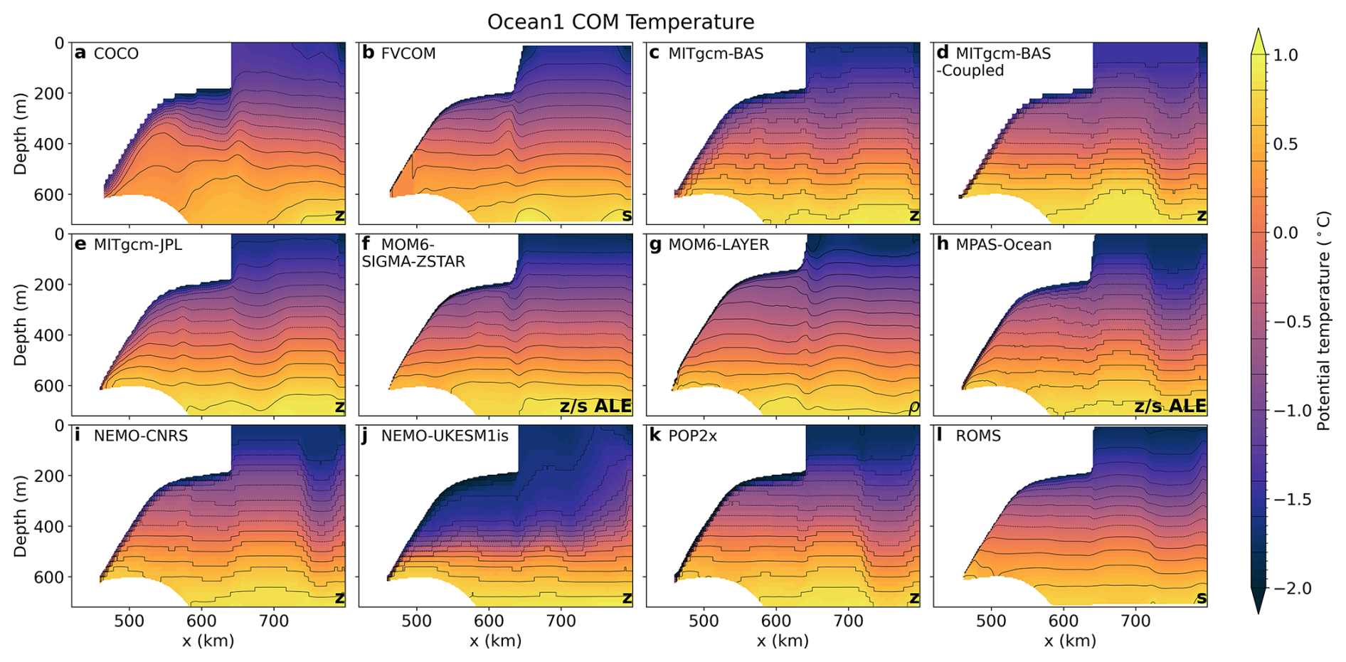
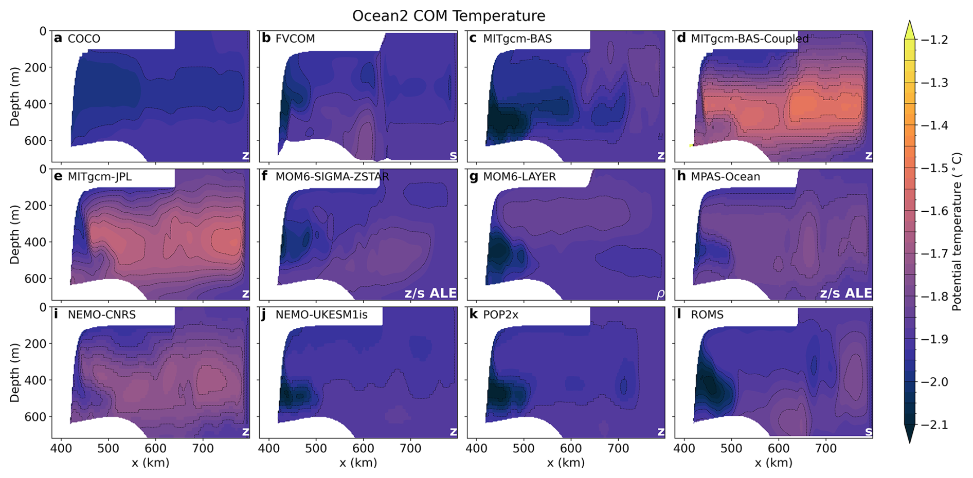
Figure 2 Spun-up (average of year 20) temperature transect along y=40 km in the Ocean1 COM experiment. Model vertical coordinates are labelled in the lower right corner, with z for z-coordinate models, s for terrain-following, ρ for isopycnal, and $z/s$ ALE for Arbitrary Lagrangian-Eulerian coordinates with a quasi z–ice shelf-following target coordinate (Table 2). Contours are spaced by 0.2 °C.

3.2 FVCOM

One submission uses the version of the unstructured grid Finite Volume Community Ocean Model (FVCOM) that resolves ice shelf cavities (Chen et al., 2003; Zhou and Hattermann, 2020). FVCOM solves the governing equations in integral form by computing fluxes between non-overlapping horizontal triangular control volumes using generalized terrain-following coordinates. In the COM submission, the model setup uses a horizontal grid mesh composed of equilateral triangles of sidelength 2 km, and 35 terrain-following vertical layers with slightly increasing resolution towards the bottom. Both momentum and tracers are horizontally advected using a second-order upwind scheme. For the vertical advection of tracers, the second-order Multidimensional Positive Definite Advection Transport Algorithm is used (Smolarkiewicz and Szmelter, 2005). To address unstable vertical mixing, salinity and temperature values in the two layers are averaged if the upper layer's density is greater than that of the lower layer. The melt rate is calculated by sampling the temperature, salinity, and velocity in the uppermost grid cell under the ice shelf. The ice shelf draft is linearly smoothed within 20 km of the ice front (Fig. 2b). The minimum water column thickness is 30 m. In addition, the bed topography in Ocean2 (seen in Fig. 3b) is further adjusted according to the water column thickness output from the ROMS model, which was first smoothed using a mean filter over a square of size 10 km side length. It was not possible to reach the target melt rate of 30±2 m yr⁻¹ below 300 m depth in FVCOM during the tuning stage in Ocean0 as melt rates saturated with high transfer coefficient values. Instead, the large value of Γ_T=0.2 chosen resulted in an equilibrium melt rate of 18.9 m yr⁻¹ in Ocean0.

Figure 3 Spun-up (average of year 20) temperature transect along y=40 km in the Ocean2 COM experiment. Model vertical coordinates are labelled in the lower right corner, as in Fig. 2. Contours are spaced by 0.05 °C. Note the different colourbar to Fig. 2.

3.3 MITgcm

Three submissions are based on the Massachusetts Institute of Technology general circulation model (MITgcm; Marshall et al., 1997), from Jet Propulsion Laboratory (hereafter MITgcm-JPL), the British Antarctic Survey (MITgcm-BAS) and a second configuration from the British Antarctic Survey that uses the coupled ice–ocean framework as described in Jordan et al. (2018) (MITgcm-BAS-Coupled). The implementation of ice shelf cavities in MITgcm is described in Losch (2008). MITgcm is a finite volume model. The configurations used here employ an Arakawa C-grid and a z-level vertical coordinate. Momentum is advected using a second-order centered scheme, while tracers are advected using a third-order Direct Space-Time (DST) flux limiter scheme (note this scheme was later found to cause some spurious behaviour, see Sect. 4.4). Differing from the COM protocol, unstable vertical mixing is parameterised with the convection scheme of Cessi and Young (1996), which instantaneously mixes the unstable density gradients, and is applied every time step. The melt rate is calculated by sampling the temperature, salinity, and velocity within a fixed 20 m boundary layer beneath the ice. Melt fluxes are also distributed over a 20 m layer beneath the ice.

The major difference between the three MITgcm COM submissions is the choice of heat and salt transfer coefficients at the ice–ocean interface (Table 2), the minimum water column thickness and the limit on the size of partial grid cells at the ice–ocean boundary. MITgcm-BAS uses a minimum water column thickness of 40 m, which is maintained by excavating the ice draft while keeping the bed topography and grounding line fixed. MITgcm-BAS-Coupled imposes a minimum water column thickness of 0.5 m for consistency with the Ocean3-4 and MISOMIP1 experiments, where the minimum water column thickness is required (Goldberg et al., 2018), with minimal effect on melt rates. The minimum size of partial cells is 25 % of a regular cell for MITgcm-JPL and 20 % for MITgcm-BAS and MITgcm-BAS-Coupled. All three configurations achieved similar, but not identical, melt rates at depth during the tuning experiment that fell within the target error margin, explained by their use of similar but not equal heat transfer coefficients and partial cell limits. The MITgcm-BAS-Coupled setup requires the use of a small (of the order of 0.05 m) minimum water column under all grounded ice in the domain (seen in Fig. 2d) to represent grounding-line retreat when used in coupled mode (Goldberg et al., 2018).

Heat transfer coefficients Γ_T for MITgcm-BAS and MITgcm-BAS-Coupled were initially reported as 0.019 and 0.021 respectively. However, subsequent analyses verifying the melt parameterisation (Sect. 4.4) revealed inconsistencies between the quoted transfer coefficients and the model output. These analyses suggested that MITgcm-BAS-Coupled used a transfer coefficient of 0.0135, and MITgcm-BAS used 0.011 in the Ocean1 experiment and 0.036 in the Ocean2 experiment (Table 2). Due to a lack of model data traceability during the intervening years, we are unable to verify which transfer coefficients these experiments used. It is hence possible that the experimental protocol was not completely followed, particularly for the MITgcm-BAS Ocean2 experiment (in the MITgcm-BAS Ocean1 experiment we can verify it achieved the tuned melt rate of 30 m yr⁻¹ averaged below 300 m depth at steady state, see Sect. 4.5). For MITgcm-BAS-Coupled we are reasonably confident that the value 0.0135 was used because we have found ISOMIP+ Ocean3 and Ocean4 simulations using that value.

3.4 MOM6

Two submissions are based on the Modular Ocean Model version 6 (MOM6; Adcroft et al., 2019). MOM6 is a finite volume model, uses the Arakawa C-grid and is formulated in a generalised vertical coordinate form. Momentum is advected using a second-order centred scheme, while tracers are advected using a piecewise linear method. Vertical mixing due to shear instabilities and convection is represented using the Jackson et al. (2008) scheme, with the critical Richardson number set to 0.25. The minimum vertical viscosity within the surface boundary layer is 10⁻² m² s⁻¹. Melting is set to zero when the total water column thickness is less than 10 m, and meltwater is added as a volume flux. The differences between the two MOM6 COM submissions are described below.

3.4.1 MOM6-SIGMA-ZSTAR

For the MOM6-SIGMA-ZSTAR configuration, the vertical coordinate is a hybrid between terrain-following (in the cavity) and z^* coordinates (in the open ocean) (Stern et al., 2017, 2019). Vertical mixing at the surface boundary layer in MOM6-SIGMA-ZSTAR is parameterised with an energetically consistent planetary boundary layer scheme (Reichl and Hallberg, 2018). The temperature, salinity and velocity used in the melt parameterisation are averaged within 20 m of the ice draft; the velocity is further averaged to the tracer grid points using the four horizontal neighbours. Sea level is maintained by adding a mass flux in the restoring region (while ensuring no change to buoyancy forcing). The ice shelf draft is smoothed using a Gaussian filter with a half-width of 2 km.

3.4.2 MOM6-LAYER

For the MOM6-LAYER configuration, the vertical coordinate is isopycnal. Vertical mixing at the surface boundary layer in MOM6-LAYER uses the bulk mixed layer scheme described in Hallberg (2003), with a minimum boundary layer thickness of 10 m. MOM6-LAYER does not use a sea level correction, so sea level increases throughout the experiment, resulting in a minor long-term drift in the melt rate of the experiments (more prominent in Ocean1) as the ocean temperature at the ice base depth is modified. The temperature, salinity and velocity used in the melt parameterisation are averaged within 10 m of the ice draft; the velocity is further averaged to the tracer grid points using the four horizontal neighbours. Meltwater is distributed into the upper layer of the bulk mixed layer. The ice shelf draft is smoothed using a Gaussian filter with a half-width of 5 km in the x-direction and 1 km in the y-direction. The ice thickness near the grounding line is decreased to maintain a minimum water column thickness of 40 m. The calving criterion (removing ice thinner than 100 m) is not applied near the ice front to minimise pressure gradient errors.

3.5 MPAS-Ocean

One submission uses the Model for Prediction Across Scales Ocean (MPAS-Ocean; Ringler et al., 2013; Petersen et al., 2018) version 6.1. MPAS-Ocean uses finite volume methods on an Arakawa C-grid. The configuration has an Arbitrary Lagrangian-Eulerian (ALE) vertical coordinate, which smoothly transitions from z^* (Adcroft and Campin, 2004) in the open ocean (with 36 vertical layers of 20 m resolution) to a terrain-following top coordinate under ice shelves. The coordinate under ice shelves constrains layer thicknesses such that the local Haney number (rx1; Haney, 1991) does not exceed a maximum value of 5. This prevents large horizontal pressure gradient errors due to the tilted vertical coordinate. Momentum is advected using a second-order, kinetic-energy-conserving scheme (Ringler et al., 2010) and tracers are advected with a third-order, flux-corrected transport (FCT) scheme (Skamarock and Gassmann, 2011). MPAS-Ocean's melt parameterisation uses temperature and salinity that are averaged within 10 m of the ice draft. The far-field ocean speed $\left|u_{\mathrm{w}}\right|=\sqrt{\mathrm{2}{E}_{\mathrm{K}}}$ is computed from kinetic energy E_K at cell centres in the layer closest to the interface, and is not averaged vertically over multiple layers. Melt fluxes (heat and freshwater) are distributed based on an exponentially decaying transmission function $T=e^{\mathrm{-}\left(z\mathrm{-}{z}_{\mathrm{d}}\right)/D}$, where z_d is the ice draft and the length scale of decay D=10 m. Sea level is approximately maintained, for all but the Ocean0 experiment, using negative freshwater fluxes applied in the northern restoring region. These fluxes are adjusted monthly, using a 3-month running mean of the meltwater flux, which was implemented offline via simple “evaporative” freshwater flux, heat flux and salt flux adjustments rather than modifying MPAS-Ocean code. The 3-month averaging window was chosen so that the lagged sea-level adjustment would not over-react to monthly fluctuations in the melt rates, though in retrospect this was likely not needed for the ISOMIP+ experiments. The provided ISOMIP+ topography was modified by smoothing with a Gaussian filter with a half-width of 2 km before interpolating to the 2 km grid. A minimum thickness of 3 layers was maintained by deepening bed topography near the grounding line.

3.6 NEMO

Two submissions are based on NEMO, the Nucleus for European Modelling of the Ocean (Madec et al., 2019): a version used at the French National Centre for Scientific Research (CNRS) (e.g., Jourdain et al., 2017) and a version used in the UK Earth System Model (UKESM,  Smith et al., 2021). The NEMO-CNRS configuration is based on a post-v3.6 release of NEMO that is described as the “COM” configuration in Favier et al. (2019), with details on the model parameters in Jourdain (2019). The NEMO-UKESM1is configuration is the “GO7” version described in Storkey et al. (2018). Both configurations use finite-difference methods on an Arakawa C-grid (Arakawa, 1966). A z^* coordinate (Campin et al., 2008) is used with a nominal uniform vertical resolution of 20 m. For a better representation of the topography, partial cells are used in the lowest and uppermost grid cells (Barnier et al., 2006; Mathiot et al., 2017). NEMO-CNRS makes use of the third-order Upstream Biased Scheme (UBS) scheme for momentum advection (flux form) and for horizontal tracer advection (Madec et al., 2019), and a second-order flux corrected transport scheme is used for vertical tracer advection. In NEMO-UKESM1is, momentum is advected in a vector invariant form, and tracers are advected with a Lax-Wendroff Total Variance Dissipation (TVD) scheme. Vertical mixing in NEMO-CNRS follows the ISOMIP+ protocol, while NEMO-UKESM1is uses a different “TKE scheme” (Madec et al., 2019), in which the background viscosity is set to the recommended stable vertical eddy viscosity and diffusivity (Table 1), with double diffusion mixing for tracers. The melt rates are calculated using temperature, salinity and velocity averaged over the top 20 m of the water column. The ice shelf meltwater and associated heat are also spread uniformly over the top 20 m. To maintain the mean sea level, ice shelf melting in NEMO-CNRS is compensated by a uniform water flux correction applied at the open ocean surface at each time step, with no associated latent heat and salt flux as described in equations 34–36 of Asay-Davis et al. (2016). In NEMO-UKESM1is, this correction was incorrectly allowed to affect the salinity of the remaining surface water. For cases of significant ice shelf melting, this issue leads to salinification of the open ocean surface and unwanted convective mixing, cooling the interior of the domain (e.g. Fig. 2j). As NEMO needs at least two vertical cells to resolve a water column, the topography is adjusted by “digging” into the ice in NEMO-UKESM1is, and equally into the ice shelf draft and the bed topography in NEMO-CNRS. Water columns of only one grid cell width in either x or y directions are also removed.

3.7 POP2x

One submission uses the Parallel Ocean Program 2 eXtended (POP2x), a version of POP2 that includes ice shelf cavities (Smith et al., 2010). POP2x uses finite-difference methods on an Arakawa B-grid. It has a z-level vertical coordinate with 20 m vertical resolution and partial top and bottom cells to represent the topography with higher fidelity. Momentum is advected using a second-order, centred scheme and tracers are advected with a flux-limited Lax-Wendroff scheme (Lax and Wendroff, 1960). POP2x's melt parameterisation uses far-field temperature and salinity, averaged over the top 20 m – from the top of the first partial cell down to the remaining required fraction of the second vertical layer. The far-field ocean velocity used in the melt parameterisation is averaged over the four neighbouring B-grid points only in the upper vertical layer. Melt fluxes (heat and freshwater) are distributed over the upper 20 m. After interpolation and removing ice thinner than 100 m, the topography is modified by (1) smoothing with a Gaussian filter with half-width of 2 km, (2) deepening bed topography near the grounding line to maintain a minimum water column thickness of 40 m, (3) either thickening or removing partial top cells thinner than 5 m, and (4) adjusting the ice draft and bed topography to ensure horizontal connectivity between neighbouring cells.

3.8 ROMS

One submission is based on the Regional Ocean Modeling System (ROMS; Shchepetkin and McWilliams, 2009), adapted to include ice shelf cavities (Dinniman et al., 2007; Galton-Fenzi et al., 2012). ROMS is a finite volume model that uses an Arakawa C-grid and a terrain-following vertical coordinate system. Only 21 vertical layers are used in the ROMS configuration, with a higher resolution near the surface and bottom. The mean top layer thickness is 0.5 m near the grounding line, 3 m at the mid-ice shelf, and 5 m near the ice front. Momentum is advected using a 3rd order upstream scheme (fourth-order centred for the barotropic momentum), and all tracers are advected using a third-order upstream scheme in the horizontal direction and a fourth-order centred scheme in the vertical. Horizontal mixing is along geopotential (i.e. horizontal, not the model terrain following) surfaces. Basal melting and freezing are computed using temperature, salinity and velocity from the top vertical layer. Heat and meltwater fluxes are distributed at the surface of the top layer only. The topography was smoothed with a 4th-order Shapiro filter to lower the maximum “slope parameter” (Beckmann and Haidvogel, 2003) to 0.1. A minimum water column depth of 20 m is used. It was not possible to reach the target melt rate of 30±2 m yr⁻¹ below 300 m depth in ROMS during the tuning stage in Ocean0, as melt rates saturated with high transfer coefficient values. Instead, the chosen value of Γ_T=0.05 results in an equilibrium melt rate of 14 m yr⁻¹.

4 Results

Here, we present the ISOMIP+ results, beginning with temperature and salinity transects, melt and circulation in the spun-up model states (Sect. 4.1, 4.2), then exploring the transient response (Sect. 4.3), differences in melt between models and their drivers (Sect. 4.4) and an alternative set of experiments where parts of the experimental protocol were relaxed (Sect. 4.5).

4.1 Spun-up temperature profiles and melt rate patterns

In this section, we present the spun-up temperature and salinity profiles and melt rate spatial distributions at the end of the Ocean1 and Ocean2 COM experiments. We take results from the average of the final year (year 20). By then, Ocean1 melt rates are approximately constant and at steady-state, but Ocean2 is still evolving and therefore still exhibits a small amount of transient adjustment (see Sect. 4.3 for further details).

Temperature and salinity distributions at year 20 of the Ocean1 and Ocean2 COM simulations at the y= 40 km transect show similarities between models (Figs. 2, 3 for temperature and Figs. 4, S8 for salinity, noting that salinity variations control the density stratification). Though Ocean1 is initialised with cold conditions, the temperature inside the cavity resembles the warm restoring conditions at the end of the simulation, with an additional cold boundary layer near the ice. Similarly, Ocean2, which is initialised with warm conditions, ends up resembling the cold restoring conditions. However, there are differences between the models; in Ocean1, NEMO-UKESM1is has a relatively colder interior (Fig. 2j), and POP2x has a colder boundary layer (Fig. 2k, see also Fig. 14k) than most other models. The cold interior of NEMO-UKESM1is can be explained by spurious convection arising from the incorrect water flux correction, as discussed in Sect. 3.6. In Ocean2, temperatures are more uniform within the domain, matching the uniform −1.9 °C sponge forcing, but MITgcm-BAS-Coupled, MITgcm-JPL and NEMO-CNRS have a warmer interior of the cavity with temperatures reaching −1.6 °C (note the different colourbar to Ocean1, which emphasises these features). This warm interior may be associated with remnant warm water from the Ocean2 warm initial conditions that have not been circulated out of the domain by the boundary forcing; that is, Ocean2 is not yet at a steady state after 20 years (see Sect. 4.3), or may indicate spurious model behaviour. These three models' counterparts MITgcm-BAS and NEMO-UKESM1is are much colder, but also have known inconsistencies with the experimental protocol (Sect. 3.3, 3.6). The coldest temperatures in all simulations range between −2.3 to −2.0 °C, lower than the coldest −1.9 °C sponge forcing temperature. These cold temperatures are generated by the melt parameterisation and occur at depth where the freezing temperature is depressed below the surface freezing point.

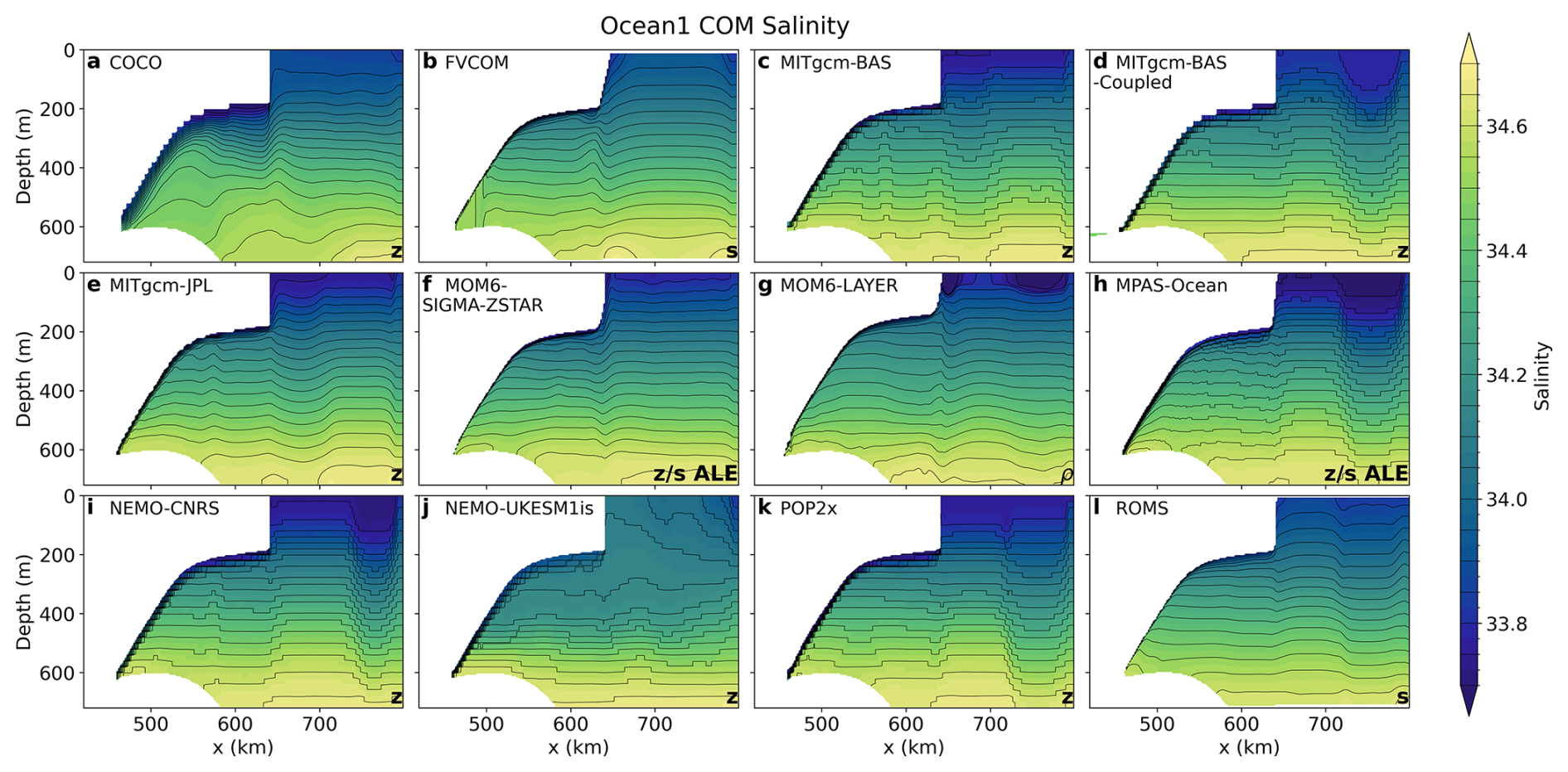
Figure 4 Spun-up (average of year 20) salinity transect along y=40 km in the Ocean1 COM experiment. Model vertical coordinates are labelled in the lower right corner, as in Fig. 2.

In the open ocean, Ocean1 temperature stratification (Fig. 2) and salinity stratification (Fig. 4) have distinct column-like features that are associated with barotropic gyres, discussed in Sect. 4.2. There is a front with a horizontal gradient in temperature below the calving front, and for some models, there is an additional front at approximately x=720 km, indicating the presence of one or two gyres.

Salinity transects in both experiments approximately indicate the density and stratification (Figs. 4, S8), which are important controllers of ocean circulation. The fresh salinity near the ice shelf–ocean boundary layer of the Ocean1 experiment indicates meltwater stratification, further highlighted by the increased density of the salinity contours near the ice. Stratification of the Ocean2 experiment (Fig. S8) is dominated by the far-field restoring forcing rather than meltwater effects, with relatively flat salinity contours. The density of the initial conditions and far-field forcings is the same for both cold and warm profiles, indicating that gradients of density are only due to meltwater interactions.

Melt rate spatial distributions in year 20 of the warm Ocean1 and cold Ocean2 COM simulations also show similarities between models (Figs. 5, 6). Melt in both experiments is enhanced at depth and near the grounding line (Fig. 7), where the thermal driving is larger. This enhancement is particularly pronounced for Ocean2, which has a steep ice shelf draft near the grounding line (Fig. 1c). Comparing Ocean1 models, the spatial distribution of melt varies, with MOM6-LAYER, MPAS-Ocean and NEMO-UKESM1is having enhanced melt at the deepest grounding line (Fig. 7a). In contrast, COCO, MITgcm-BAS-Coupled and MOM6-SIGMA-ZSTAR have enhanced melt at the cavity sidewalls (Fig. 5). FVCOM has a region of freezing on the +y side wall. Additionally, POP2x has a pronounced checker-board melt pattern. This striped pattern is also visible to a lesser extent in the other z-level coordinate models COCO, MITgcm and NEMO. For Ocean2, melt rates away from the deepest grounding line are small but COCO and FVCOM simulate significant freezing at the side walls (Fig. 6). COCO and FVCOM also have larger melting at depth near the grounding line (Fig. 7b) and also have cold temperatures near the ice base of the y=40 km transect (Fig. 3). Other models (e.g. MITgcm-BAS, MOM6-LAYER, NEMO-UKESM1is, POP2x, ROMS) also have cold temperature transects (i.e. lack the warm temperatures remnant from the spin-down observed in some models, Fig. 3) and no such freezing, however, the temperature transects do not sample the sidewall region where freezing occurs. These variations demonstrate that models can achieve similar cavity-averaged melt rates (the tuning target melt rate below 300 m is achieved by all models except ROMS and FVCOM) with very different spatial distributions of melting. These differences in melt rate patterns, particularly near the grounding line and side walls, are likely to be at least partly associated with differences in representations of bed topography and ice shelf draft between models that are enhanced near the side walls, grounding line and ice front (Figs. S11, S12). Differences in spatial distributions of melting have implications for ice sheet evolution in coupled ice sheet–ocean models as the ice thickness and therefore the buttressing effect may evolve differently depending on the location of melt.

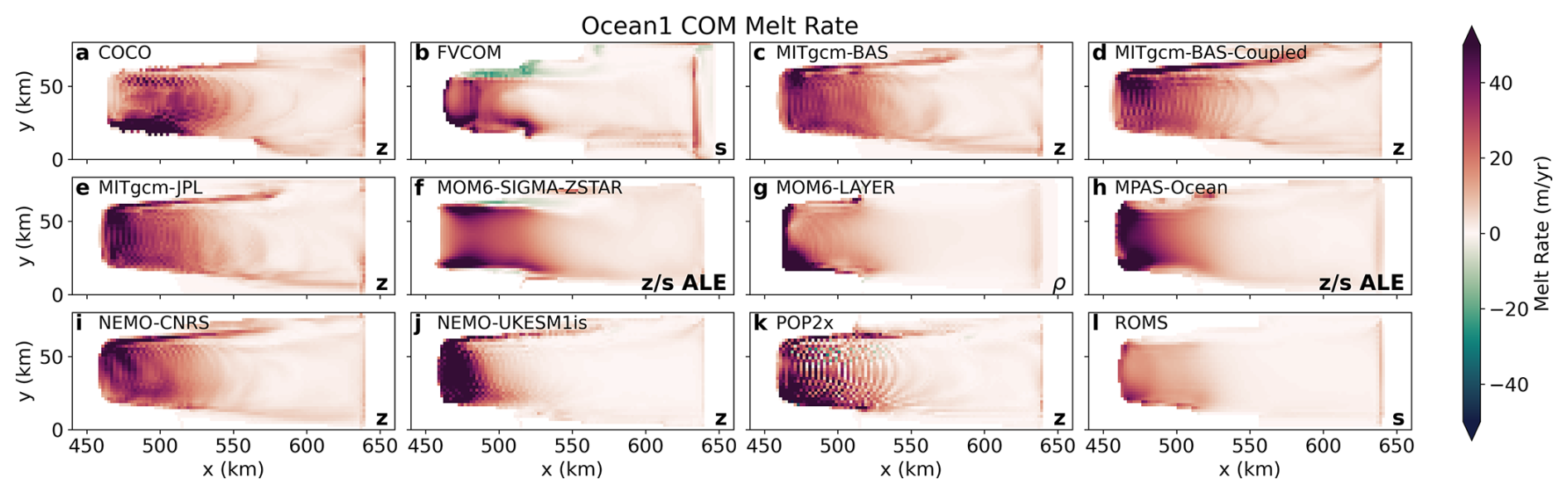
Figure 5 Spun-up (average of year 20) melt rate spatial distributions for each of the 12 models in the Ocean1 COM experiment, corresponding to a warm cavity state. Model vertical coordinates are labelled, as in Fig. 2.

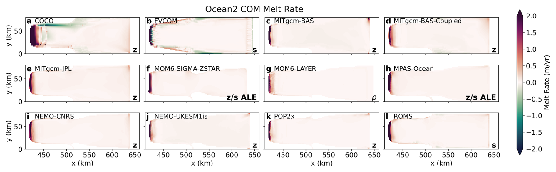
Figure 6 Spun-up (average of year 20) melt rate spatial distributions for each of the 12 models in the Ocean2 COM experiment, corresponding to a cold cavity state. Model vertical coordinates are labelled, as in Fig. 2.

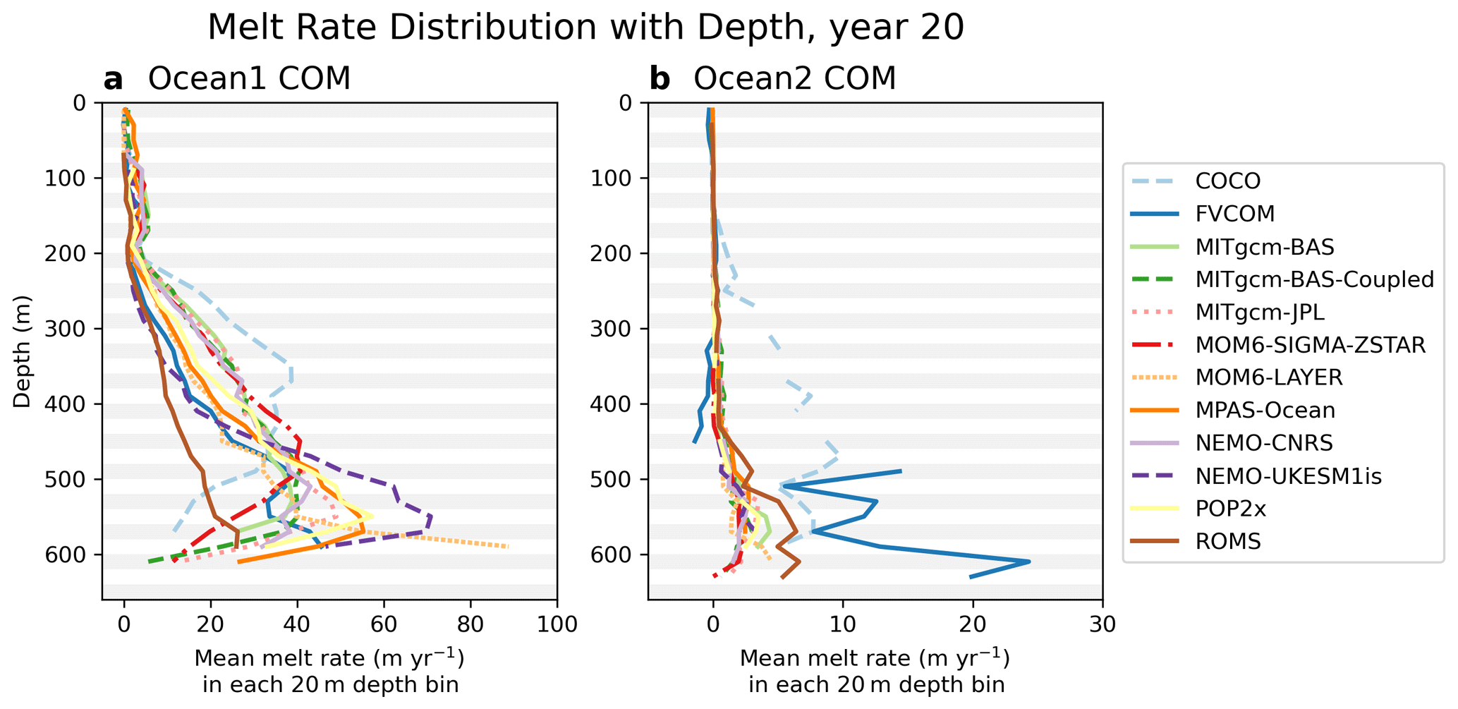
Figure 7 Melt rates averaged over year 20 as a function of ice depth, for (a) the Ocean1 COM (warm) and (b) the Ocean2 COM (cold) experiments. The two experiments have different geometries, Ocean2 having a steeper ice base slope over a narrower x-axis extent than Ocean1. Due to the discontinuous vertical axis and differences in ice draft between models, we plot the average melt rate in 20 m sized depth bins, indicated by the grey and white bars. Discontinuities occur when no regions of the model's ice draft are within a 20 m bin.

4.2 Spun-up circulation

We present the overturning and barotropic streamfunctions for the Ocean1 and then Ocean2 COM experiments during year 20, where models are spun up. Ocean1 is approximately at steady state, but Ocean2 still exhibits some transient adjustment. Further calculation details are in Asay-Davis et al. (2016). The overturning streamfunction is presented in x–depth coordinates due to model data availability: using density coordinates may have allowed better quantification of water mass transformations in the ice shelf cavity (Webber et al., 2019), but circulations are qualitatively similar (see, e.g. Fig. 4 in Yung et al., 2025, but note they use smaller transfer coefficients and have lower melt rates than the ISOMIP+ protocol). Future model intercomparisons should consider including the density-coordinate overturning streamfunction as a required diagnostic, and may also consider diagnosing adiabatic and diabatic contributions to heat transport.

The overturning circulations in year 20 of the warm Ocean1 experiments show common features across models (Fig. 8), with upwelling occurring in the ice shelf cavity and downwelling near the northern boundary. The strength of the overturning varies between models, with most models showing maximum streamfunction values of 0.20–0.25 Sv. COCO demonstrates the strongest overturning streamfunction, with a peak value of 0.39 Sv, whilst ROMS and FVCOM have weaker circulation which is likely attributed to lower melt rates (Fig. 5, see also Fig. 12). The structure of the overturning streamfunction also varies, with some models displaying two distinct peaks, one within the ice shelf cavity and another near the “northern” (x= 800 km) boundary (e.g., MITgcm-BAS-Coupled, MITgcm-JPL, NEMO-CNRS), and others exhibit a single peak near the northern boundary (e.g., FVCOM, MITgcm-BAS, MPAS-Ocean, POP2x, ROMS). Varying bed topography and ice geometry in both x and y-direction (Fig. 1) results in the streamfunction, which is computed by averaging velocities over the y-direction, being nonzero in (x,z) coordinates that are not simulated as ocean in the y=40 km transect (e.g. Fig. 2).

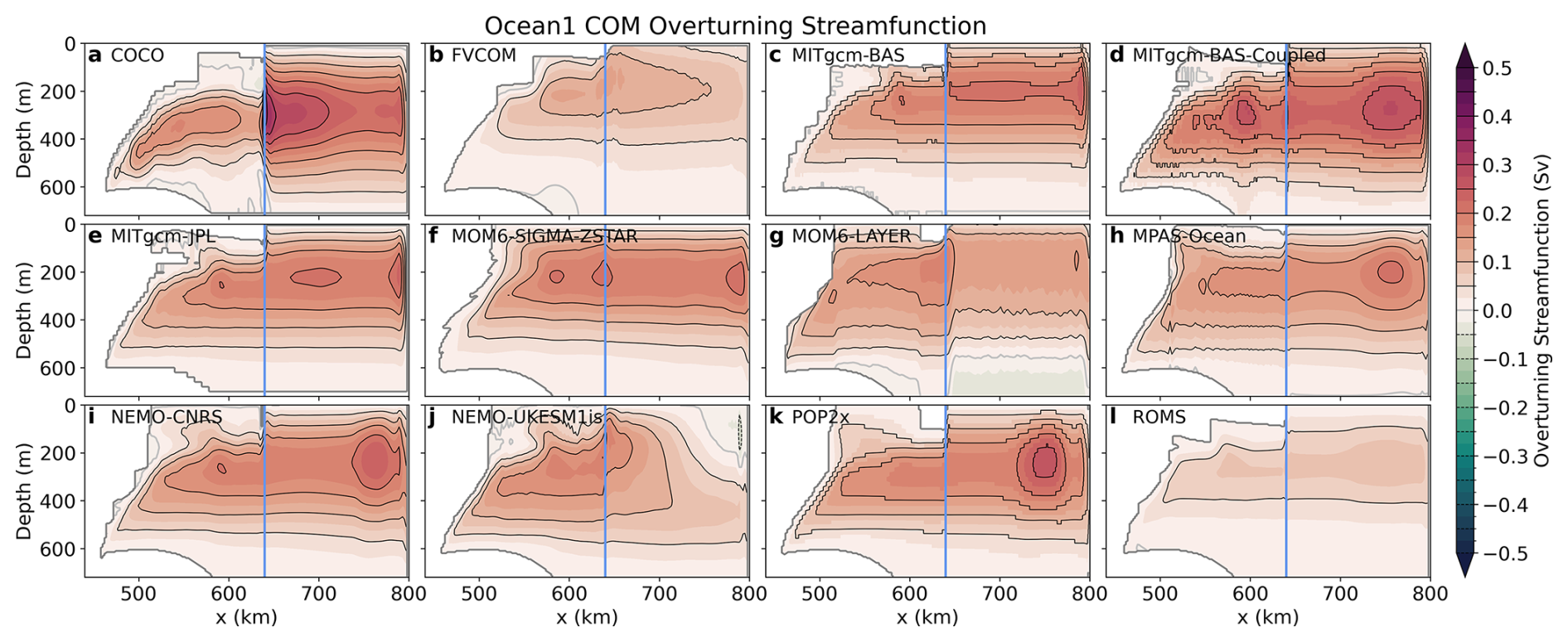
Figure 8 Ocean1 COM overturning streamfunctions in depth–x coordinates, averaged over the y direction and over year 20, corresponding to the steady warm state of the cavity. The 0 Sv contour is indicated by a light grey line and the ice front at x=640 km is indicated by a blue line.

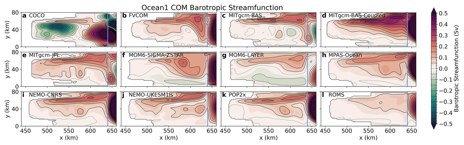
Figure 9 Ocean1 COM barotropic streamfunction averaged over year 20, corresponding to the steady warm state of the cavity. We restrict the range of the x-axis to the ice shelf cavity; an extended version is shown in Fig. S5. The 0 Sv contour is indicated by a light grey line and the ice front at x=640 km is indicated by a blue line.

The barotropic streamfunctions in year 20 of the warm Ocean1 experiments reveal similar circulation patterns across most models within the ice shelf cavity, with the exception of COCO (Fig. 9 in the ice shelf cavity and see Fig. S5 for the full domain). The typical pattern involves a boundary-intensified (y>50 km) clockwise, cyclonic circulation within the cavity, with a maximum barotropic streamfunction of 0.26 ± 0.17 Sv in this region (y>50 km, x<640 km). The circulation feature varies in shape, with some models having strongly boundary-intensified circulation (e.g. MITgcm-BAS) while others are centred further away from the boundary (e.g. MOM6-SIGMA-ZSTAR), and the extent that the circulation penetrates towards the grounding line also differs between models. However, COCO deviates from this pattern, with only a weak boundary flow and instead a strong counterclockwise circulation within the ice shelf cavity. This circulation is potentially linked to a spatial pattern of ice shelf melt with peaks along the “eastern” (y<30 km) boundary of the ice shelf cavity, in contrast to many other models (Fig. 9). In this eastern region of the ice shelf cavity, there are differences in circulation between all models (e.g. differences in location of the grey, solid 0 Sv line in Fig. 9), and in particular, the MOM6 models display a large counterclockwise circulation. Variation in circulation between models may be associated with the different interpolation and smoothing choices of the bed topography and ice shelf draft, particularly near the side walls, grounding line and ice front (Sect. 3, Figs. S11, S12) and are likely also related to the different melt rate spatial distributions (Figs. 5, 6, 7).

Moving further towards the open ocean, the warm Ocean1 barotropic streamfunctions show a clockwise inflow and outflow of water crossing beneath the ice shelf calving front at x= 640 km. This flow, quantified by the maximum barotropic streamfunction near the ice front (630 km $<x<$ 650 km), varies in magnitude (0.41 ± 0.27 Sv), with models with higher barotropic streamfunctions also typically having higher overturning streamfunctions. Despite the general similarity in ocean circulation within the ice shelf cavity, the ocean circulation outside the ice shelf cavity shows significant variability among the models, and is generally stronger in magnitude (Fig. S5). Some models have two open ocean gyres, with no consistent rotation direction between models, whilst other models (e.g. FVCOM, MOM6-SIGMA-ZSTAR) have just one gyre (and the number of gyres can vary with time). These open ocean gyres are sensitive to the discretisation of the ice shelf geometry in the MISOMIP1 configuration (Zhao et al., 2022) and may also be sensitive to the model implementation of the northern boundary restoring region.

In the cold and steep ice base Ocean2 experiments at year 20, the overturning circulation consists of an opposing two-cell structure across most models, with a clockwise, cyclonic circulation at deeper levels and a counterclockwise circulation at shallower depths (Fig. 10). This circulation can be explained by a buoyant meltwater current that rises beneath the steep ice base near the grounding line until it reaches its neutral buoyancy and separates from the ice shelf (Holland, 2017). Return flow above and below this depth is created by the modifications made by the restoring forcing to the fluid's buoyancy at the x=800 km wall boundary and is constrained by conservation of volume. The similar cell separation height across models (grey solid line in Fig. 10) suggests that the neutral buoyancy depth places a strong constraint on the vertical overturning structure, especially since the salinity stratification is strong (Fig. S8). Typical circulation strengths are 8.2±2.4 mSv for the deep clockwise circulation and $-\mathrm{7.6}\pm \mathrm{2.4}$ mSv for the shallower counterclockwise circulation for all models except COCO and FVCOM. COCO and FVCOM show overturning strengths about 14 and 3 times larger than the other models, respectively. The separation of the meltwater current from the ice draft at its neutral buoyancy depth also explains the lack of freezing in the models (Fig. 6). Note that the simulated shallow counterclockwise circulation is likely related to density gradients in the domain that develop in response to the boundary restoring to the salinity-stratified cold profile, in combination with the steep ice base geometry, rather than local buoyancy fluxes (which are small due to the low melting at shallow depths, Fig. 6). The circulation is a feature of our model setup, noting the unrealistically strong stratification and that reversed overturning cells of this extent have not been observed in Antarctic ice shelf cavities (to our knowledge). However, the counterclockwise circulation may not be completely unrealistic since mixed-source circulation and a surface inflow of shelf water have been observed at cold cavity ice fronts (Hattermann et al., 2021; Janout et al., 2021) and observations of large-scale currents beneath Antarctic ice shelves remain limited.

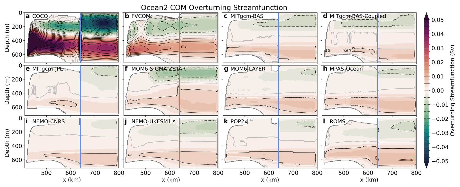
Figure 10 Ocean2 COM overturning streamfunctions in depth–x coordinates, averaged over the y direction and over year 20, corresponding to the steady cold state of the cavity. The 0 Sv contour is indicated by a light grey line and the ice front at x=640 km is indicated by a blue line.

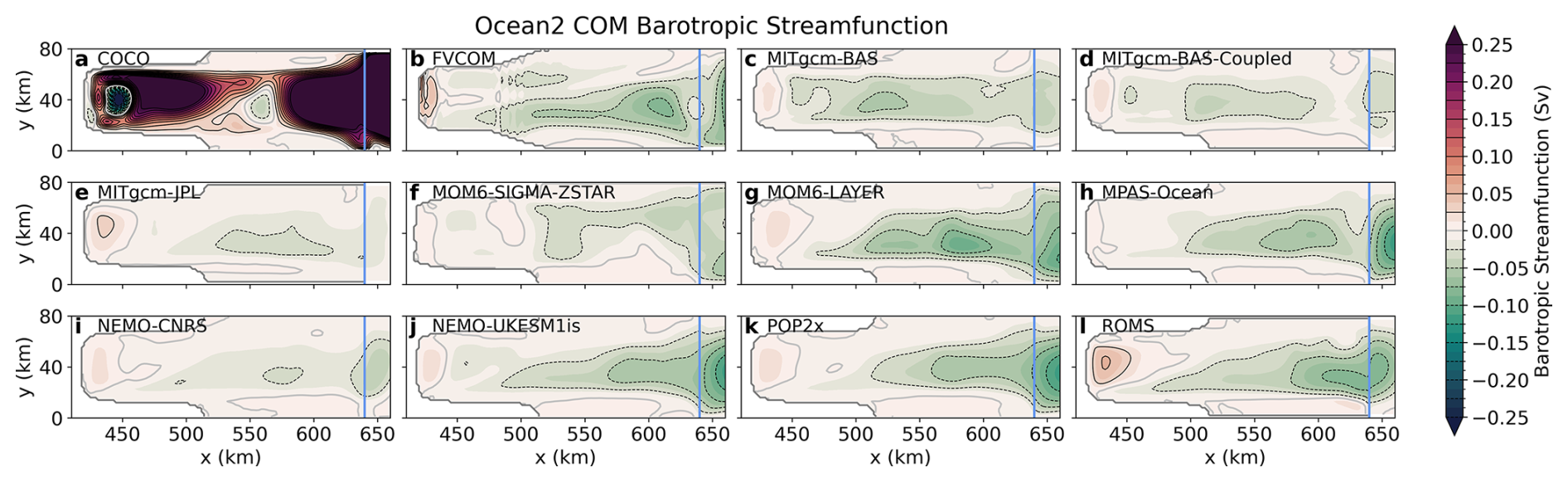
Figure 11 Ocean2 COM barotropic streamfunction averaged over year 20, corresponding to the steady cold state of the cavity. We restrict the range of the x-axis to the ice shelf cavity; an extended version is shown in Fig. S6. The 0 Sv contour is indicated by a light grey line and the ice front at x=640 km is indicated by a blue line.

The barotropic streamfunction in the cavity (Fig. 11; see Fig. S6 for the full domain) at year 20 of the cold Ocean2 experiments generally shows a similar circulation pattern across models, except for COCO. Most models exhibit weak clockwise circulation near the grounding line (maximum streamfunction for x< 460 km is 47 ± 42 mSv) and counterclockwise circulation in the outer ice shelf cavity (minimum negative streamfunction inside the cavity for x> 460 km is −75 ± 43 mSv), though circulation patterns differ. In contrast, circulation in COCO once again differs significantly from other models, consisting of two strong clockwise circulations within the ice shelf cavity. These circulations have peaks in both the inner and outer cavity, showing circulation strengths of 0.29 and 1.2 Sv, respectively. Despite the similarities in simulated ocean circulation within the ice shelf cavities, the circulation patterns outside the ice shelf cavity differ significantly (Fig. S6), consistent with the findings from the Ocean1 experiment.

The circulation results for both the Ocean1 and Ocean2 experiments suggest that (a) most ISOMIP+ ocean models are capable of simulating similar ocean circulation structures within the ice shelf cavity, which are only weakly influenced by the off-shelf ocean circulation, underscoring the robustness of these models, and (b) differences in the treatment of ocean boundaries and sponge layers among the models and model geometries may contribute to the observed discrepancies.

4.3 Transient melting

In this section, we explore the transient nature of the ISOMIP+ Ocean1 and Ocean2 COM ice shelf cavity experiments where the ocean's initial conditions adjust to the forcing at the northern boundary. The melt rate changes as temperature and salinity changes are advected into the cavity, and there are feedback mechanisms between melting and the barotropic and overturning circulation.

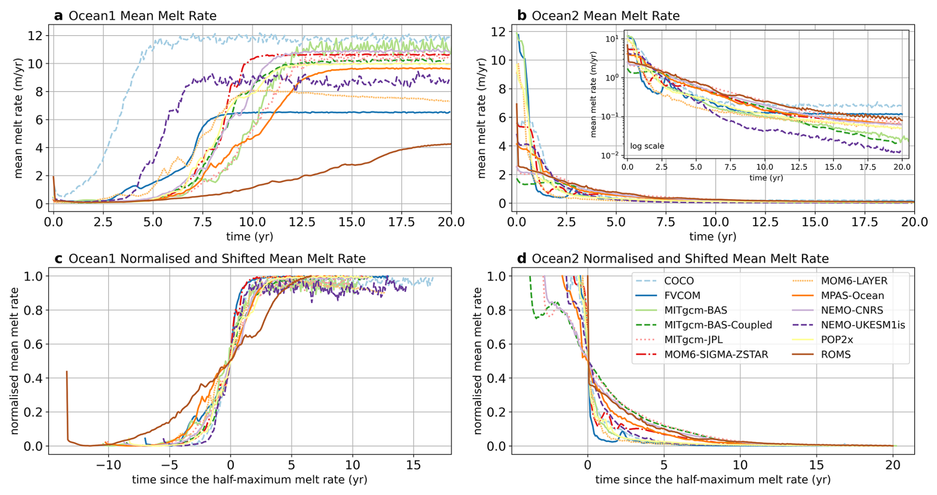
Figure 12 Area-averaged melt rate over the entire ice shelf for the (a) Ocean1 COM and (b) Ocean2 COM experiments, showing a spin-up and spin-down respectively of the overturning circulation over time. Panels (c) and (d) normalise the melt rate by the maximum melt rate and shift the time axis such that their midpoints are at time zero for each experiment.

The area-averaged melt rates over the entire ice shelf for the Ocean1 and Ocean2 experiments as a function of time demonstrate the dependence of melt rate on ocean conditions and circulation (Fig. 12). The Ocean1 melt rate increases from its low baseline created by the cold initial conditions as the warm boundary forcing penetrates the cavity. Melt rates approach a constant value for all models by year 14, except for ROMS which is still increasing in year 20 (Fig. 12a). The quasi-steady mean melt rates vary significantly across models (4–12 m yr⁻¹) and some models (COCO, MITgcm-BAS, NEMO-UKESM1is and MPAS-Ocean) show larger temporal variability in melt rate with ∼ 1 m yr⁻¹ variation in the monthly averaged data. These maximum area-averaged melt rates are lower than the target 30 m yr⁻¹ of the Ocean0 tuning experiment, which matches the steady state Ocean1 conditions, because the Ocean0 tuning only considers the ice shelf cavity regions deeper than 300 m (recall that all models except FVCOM and ROMS achieved the Ocean0 target melt rate). The large variation in the final ice shelf cavity-averaged melt rate highlights the importance of the spatial distribution of melt (Fig. 5a), particularly as a function of depth (Fig. 7). Additionally, the time taken for the model spin-up to reach a steady state varies between the models, with COCO reaching steady melt rates within 5 years but ROMS still increasing in melt at year 20. However, after an initial spin-up phase, most models show a similar transition time during which the melt rates increase in response to the warming cavity, as demonstrated in Fig. 12c. Here, the melt rates are normalised by their maximum value and shifted by the earliest time they achieve a melt rate of half their maximum melt rate. The models merge into one sigmoid-like profile with an approximate width of 5 years, except for ROMS. This similarity indicates that differences in spin-up time are more likely to be associated with the timescales for which the boundary forcing propagates into the ice shelf cavity rather than different circulation responses to changing melt rates.

The Ocean2 melt rates decrease from relatively high values, due to the warm initial conditions, towards melt rates of less than 2 m yr⁻¹ within 2 years, in response to the advection of the colder water from the restoring into the cavity (Fig. 12b). The logarithmic scale inset demonstrates that the resultant melt rates at 20 years still vary by an order of magnitude between 0.01–0.2 m yr⁻¹, and additionally that many of the models have not yet reached steady state, a possible explanation for the remnant warm temperatures in some of the year 20 temperature transects (Fig. 3). When scaled and shifted in time (Fig. 12d), the models are similarly described by a sigmoid-like profile, though there are some exceptions with a rebound in melt rate in MITgcm-BAS-Coupled and MITgcm-JPL after ∼ 2 years, possibly related to the development of a melt-circulation feedback or a result of the advection scheme producing spuriously warm water (Sect. 3.3).

The different initial (slower) spin-up and (faster) spin-down timescales in the Ocean1 and Ocean2 experiments, respectively (Fig. 12), can be explained by the timescales of advection of temperature anomalies by the overturning circulation, as well as the differing ice geometries in the two experiments. Since the boundary conditions and initial conditions have the same density stratification (Fig. 6 of  Asay-Davis et al., 2016), the only source of density variations is ice shelf melting (Holland, 2017), which is guided by the temperature of the cavity. In the Ocean1 simulation, warm water is slowly advected from the boundary to the base of the initially cold Ocean1 ice shelf by the weak cold cavity state circulation, leading to low melt rates for ∼ 5 years for most models. Once warm intrusions arrive at the ice shelf base, they drive increased melt and buoyancy-driven overturning, which advects warm boundary water into the cavity more quickly in a feedback mechanism that further spins up the circulation. The colder-restoring Ocean2 begins with a fast warm cavity state circulation, rapidly slowed by the cold temperature intrusion as the melting drops, to become a weak circulation. The flow also separates from the ice at mid-depth (Fig. 10), further reducing melt and circulation. The slower circulation in Ocean2 therefore increases the time required to “flush” the cavity with the boundary conditions and equilibrate, explaining why most models have reached a steady state by the end of Ocean1, but not Ocean2. Additionally, the difference in ice base geometries between Ocean1 and Ocean2 (Fig. 1) likely contributes to this asymmetric behaviour. However, similar asymmetries in warming and cooling transient melt rate responses are seen in fixed geometry simulations with an oscillating far-field forcing, such as in the Ocean1 domain (Zhou et al., 2024) and in wedge-like ice shelf setups (Holland, 2017).

We also compare the relationship between ocean temperatures and melting. For the Ocean2 experiments, area-averaged melt rates scale approximately quadratically with ocean temperatures near the front of the cavity (or more specifically, the thermal forcing at the front of the cavity, taken as the difference between the ocean temperature and a reference freezing point at depth of −2.1 °C, has a log-log best-fit power-law exponent with melt of n≈2 on average in Fig. S1b). This relationship is consistent with the quadratic equilibrium response of the melt rate to thermal forcing shown in Holland et al. (2008) and Holland (2017). The Ocean1 simulations have a different scaling (close to linear with n≈1.3, see Fig. S1a) associated with the cavity being in a transient state. This transient state can be explained by the observed delay in spin-up due to weak circulation despite warming ocean temperatures near the front of the cavity. The deviation from the quadratic scaling is consistent with Holland (2017), who show that warm-to-cold transitions (i.e. Ocean2) better match the equilibrium response (a quadratic melt rate–thermal driving relationship) compared with cold-to-warm transitions (i.e. Ocean1).

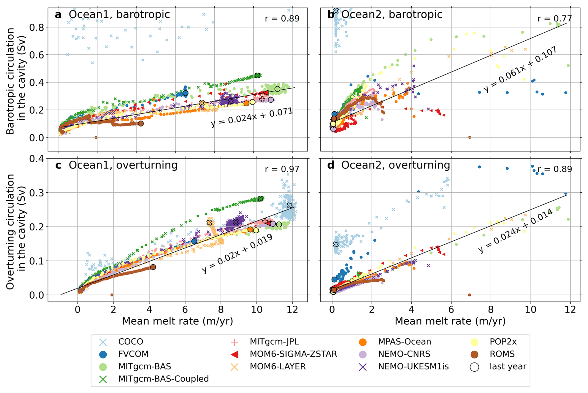
Figure 13 Strength of the barotropic (upper) and overturning (lower) streamfunctions as a function of area-averaged melt rate for the Ocean1 COM experiments (left) and Ocean2 COM experiments (right). Circulation strength is determined from the maximum minus minimum streamfunction values in the cavity, i.e. for x< 640 km. Each scatter point represents a different month of data. Linear lines of best fit and Pearson correlation coefficients include all data except for the COCO model. In some panels, COCO results fall outside the main range of the other models.

The ISOMIP+ experiments demonstrate a strong relationship between melt rate and circulation across models and forcings. Fig. 13 shows the barotropic and overturning circulation strength, calculated from the difference between maximum and minimum streamfunction amplitudes within the ice shelf cavity, as a function of area-averaged melt rate for each month of the Ocean1 and Ocean2 simulations. Most models follow shared linear relationships between melt rate and overturning and barotropic streamfunctions for both the Ocean1 and Ocean2 experiments. Consistent with previous circulation metrics (Figs. 9 and 11), the COCO barotropic streamfunction is abnormally strong in both experiments, suggesting the influence of a circulation source other than melting. Deviation from the linear relationship between melt and circulation strength may be explained by the circulation being influenced by the restoring at the boundary in addition to the expected buoyancy forcing from melting. If the ice shelf cavity flow is driven only by buoyancy, the magnitude of melt would be expected to be proportional to the near-ice velocity, which in turn should scale (to first-order) with overturning circulation strength (e.g. MacAyeal, 1984; Jourdain et al., 2017), noting that melt rate feedbacks on stratification would modify this relationship. In this buoyancy-driven flow regime, the barotropic ice shelf cavity flow is mostly geostrophic and driven by the density difference between the buoyant meltwater and deep ocean restoring water properties, therefore, barotropic flow would also scale linearly with melt (e.g. Jenkins, 2016; Jourdain et al., 2017; Finucane and Stewart, 2024). However, note that geostrophy does not hold near boundaries due to the presence of boundary drag, but the boundaries of the ice shelf cavity contain regions with significant melt (e.g. y>60 km in Fig. 5). Understanding the ocean dynamics involved in the coupled melt rate–circulation relationship requires further experiments not performed here.

Despite both Ocean1 and Ocean2 having linear circulation–melt relationships, correlations are weaker in Ocean2 (Fig. 13b, d). The overturning metric in Ocean2 quantifies the speed of the mid-depth flow away from the ice shelf as the meltwater flow separates from the ice (Fig. 10), and is therefore less tightly coupled to the melt rate averaged across the whole ice shelf than in Ocean1. Additionally, the reduction in the strength of the correlation between melt and circulation in Ocean2 may be due to weaker circulation strength, which would increase the importance of boundary layer temperature and salinity properties that change with melting. The prescribed tidal friction velocity (acting to increase the melt compared to that expected by the boundary layer velocity) may contribute to the non-zero intercepts of the circulation–melt relationships, which is more prominent in the slower Ocean2 experiments (Fig. 13).

Despite the deviations in some models from the linear circulation–melt relationship, Fig. 13 demonstrates agreement in the circulation–melt relationship amongst the models. This model agreement is promising, showing reliability in simulated ocean-ice interactions and feedback processes between circulation and melt. The circulation–melt relationship is thus an important metric for model comparison, where models display agreement despite individual melt rate or temperature distributions.

4.4 Differences and drivers of melt rate

Many of these differences in melt rate between models can be understood by considering the driving factors of ice shelf basal melt. Much of these differences can be attributed to (a) the differences in the representation of the temperature and salinity properties in the boundary layer region, and (b) model choices of calculating the thermal and haline driving and the distribution of heat and meltwater fluxes.

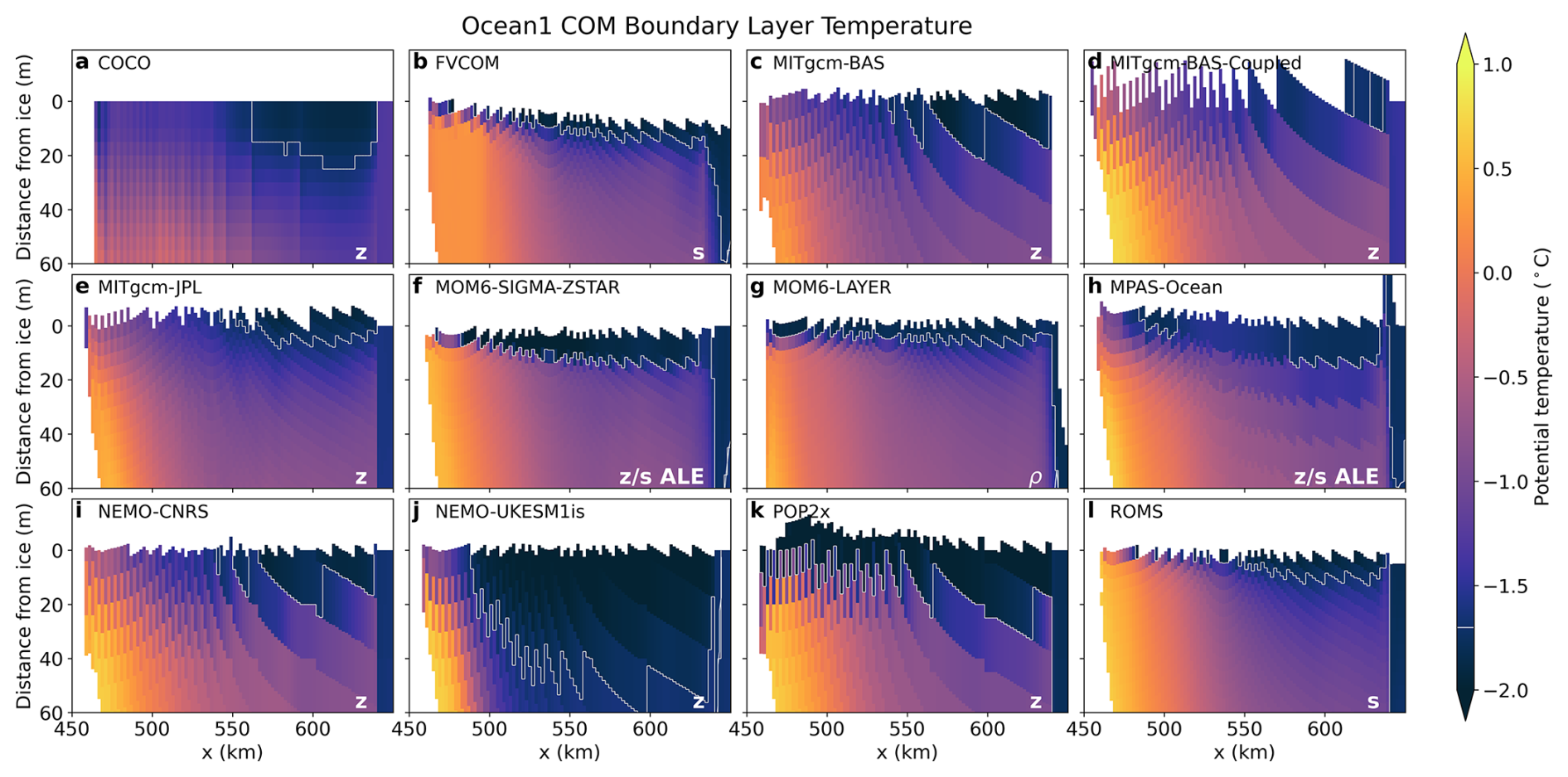
Figure 14 Boundary layer temperature transect, averaged over year 20 of the Ocean1 COM experiment. The temperature transect of Fig. 2 is remapped in the vertical direction to be the distance away from the ice (taken from the difference between the remapped model output on a 5 m resolution grid to the ice draft, which can be values not on the 5 m grid, leading to jagged shapes; see Fig. S13). Model vertical coordinates are labelled, as in Fig. 2. The −1.7 °C contour is shown in white.

The representation of the ice shelf–ocean boundary layer in the Ocean1 COM models at year 20 is shown in Fig. 14, when the cavity is in a warm state. Here, we show the potential temperature in the upper ice shelf cavity, where the vertical coordinate is the distance from the ice shelf basal surface. This remapping produces the jagged features of Fig. 14: model output is remapped onto a discrete grid with 5 m vertical spacing, relative to 0 m depth, whereas the ice draft used in each model can vary continuously. Therefore, the distance from the ice (the difference in depth, i.e. the difference between ice draft crosses and 5 m output in Fig. S13) has both discrete and continuous components and is jagged in shape. Additionally, the distance can be negative if the depth to which the ocean model output is remapped is shallower than the ice draft (e.g. MITgcm-BAS-Coupled, Fig. S13d).

Comparing boundary layer temperature profiles, most Ocean1 models show warmer water at depth away from the ice base (Fig. 14). Conditions are particularly warm (greater than 0.5 °C) near the ice base in the deeper portions of the cavity (e.g. x-coordinate of 450–500 km), but models show different widths in the x-direction of this warmer water band. Upslope of this warm region (x>500 km), there is a transition to cooler temperatures (∼ −1.1 to −0.025 °C). Above this, and directly below the ice shelf, there is a cold layer (the ice shelf meltwater; approximately $<-\mathrm{1.7}$ °C, shown in white contours in Fig. 14). All the Ocean1 COM models simulate these features but with different horizontal and vertical scales. Ice shelf–ocean boundary layers in the cold Ocean2 COM models are colder and thicker than Ocean1, but also exhibit inter-model variation (Fig. S2) and may be associated with the models not yet reaching equilibrium (Figs. 3, 12).

Focusing on the meltwater layer closest to the ice shelf–ocean boundary, Ocean1 COM models have different temperature profiles (Fig. 14; see Fig. S2 for Ocean2 COM results). Some models have a thin, cold layer that transitions smoothly and relatively rapidly into warmer water below, e.g. FVCOM, MITgcm-JPL, MOM6-SIGMA-ZSTAR, MOM6-LAYER and ROMS: mostly the terrain-following and isopycnal coordinate models (note the 5 m resolution output may also hide part of the thin, cold boundary layers in ROMS and FVCOM, e.g. ROMS has top layer thicknesses less than 5 m). Some models have a cold layer but with a thicker extent (MITgcm-BAS, MITgcm-BAS-Coupled, MPAS-Ocean, NEMO-CNRS and NEMO-UKESM1is). Sharp differences in temperature along the meltwater layer suggest that the z-coordinate resolution and its step-like boundary are partially responsible. Lastly, some other models have a largely unique representation of the boundary layer, being much thicker than the other models (COCO and NEMO-UKESM1is, the latter of which has known erroneous surface cooling). POP2x also has a very cold boundary layer, which explains why it requires such a large melt rate transfer coefficient (Table 2) compared to other z-coordinate models to achieve the same target melt rate, and may indicate numerical inaccuracies. Boundary layer representations are therefore dependent on the vertical coordinate, with terrain-following coordinates tending to have thinner boundary layers, likely due to their higher vertical resolution beneath the ice shelf and reduced implicit mixing (in models that distribute meltwater over only the uppermost layer). Meltwater fluxes stably stratify the water column, hence thin, stratified boundary layers have potential feedback effects on melt rate. However, other model-specific numerics may also play a role, noting significant differences in boundary layer representation even between z-coordinate models with the same vertical resolution. These differences may be associated with different implementations of the Losch (2008)-style sampling and meltwater distribution layer, as well as partial cell thicknesses. The simplified, prescribed diffusivities of the ISOMIP+ COM protocol may also be an important controller of boundary layer representation compared to model mixing parameterisations used in typical realistic model configurations (equivalent results for TYP configurations shown in Figs. S9, S10). In summary, Fig. 14 demonstrates that the ice–ocean boundary temperature profile is a key metric of variability between models.

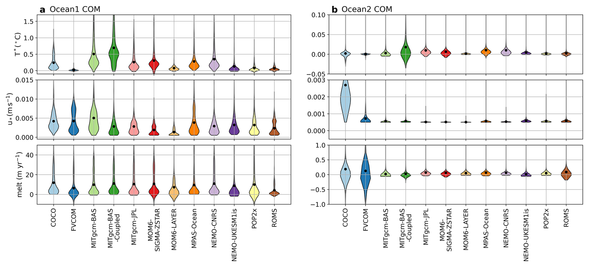
Figure 15 Statistical distributions in space of thermal driving (T^*), friction velocity (u_*) and melt for each model and Ocean1 and Ocean2 COM experiments, averaged over year 20. Black dots represent the spatial mean values.

Ice shelf–ocean boundary layer temperature is one controller of melting that differs between models. However, the strength of the friction velocity is also included in the basal melt parameterisation, as are the transfer coefficients. Fig. 15 shows the distribution of thermal driving (defined as the difference between the far-field and boundary layer temperature in the melt parameterisation; $T_{\mathrm{w}}-T_{z_{\mathrm{d}}}$ in Eq. 3), friction velocity and melt over the cavity averaged over year 20, noting that the product of thermal driving and friction velocity is scaled by the transfer coefficients (which differ between models) and other constants to determine melt. Thermal driving in Ocean1 is generally larger in the models with thicker boundary layers, mostly z-level models that use a 20 m layer to sample temperature and salinity that may extend deeper into the warm cavity interior than the meltwater layer (e.g. COCO, MITgcm-BAS, MITgcm-BAS-Coupled, MITgcm-JPL and NEMO-CNRS). z-level models also tend to have slightly larger friction velocities, possibly also associated with a deeper sampling depth. The spatial distribution of melt rates with depth (Fig. 7) is associated with both thermal driving and friction velocity distributions, where model variation in the location of peak melt rate is associated with the friction velocity (and therefore circulation) as well as increasing thermal driving with depth. In Ocean2, there are large differences in the distribution of thermal driving, whereas friction velocities are small and for all but COCO (which has an anomalously strong barotropic circulation, Sect. 4.2) display a nearly spatially uniform friction velocity of $\mathrm{5}\times {\mathrm{10}}^{-\mathrm{4}}$ m s⁻¹, which is the minimum prescribed tidal velocity scaled by the drag coefficient. Fig. 15b also highlights the significant portions of the COCO, FVCOM, ROMS and MITgcm-BAS-Coupled cavities that are freezing at the ice shelf-ocean interface rather than melting.

One of the key parameters in the experiment is the heat and salt transfer coefficients of the three-equation parameterisation, which control the melt rate and, therefore, circulation. To verify the implementation of the basal melt parameterisation, diagnosed melt rates (and hence applied meltwater fluxes) are compared with the product of the diagnosed thermal driving and friction velocity in the Ocean1 and Ocean2 COM models (Fig. S3). The melt rate is scaled by constants in Eq. (3), including model-dependent transfer coefficients (Table 2). POP2x shows some deviations from the diagonal 1:1 line, possibly indicating transient numerical inaccuracies. The MITgcm-BAS-Coupled simulation has a slope of 1 only if a readjusted transfer coefficient is used rather than the value initially reported (see Sect. 3.3 for more details), as does the Ocean1 simulation of MITgcm-BAS, which has a systematically different slope from the Ocean2 simulation. As discussed in Sect. 3.3, the transfer coefficients used may have differed from the reported values, or there was a diagnostics error. Nevertheless, the z-level models tend to have similar thermal transfer coefficients between 0.0135 and 0.0325 (Table 2) with some exceptions: NEMO-UKESM1is requires a larger coefficient to offset its erroneous cooling, MITgcm-BAS has inconsistent transfer coefficients, and POP2x has an anomalously large transfer coefficient that we do not have an explanation for. The other z-level model configuration transfer coefficients are generally smaller than that for the terrain-following, ALE and isopycnal coordinates (Table 2). z-level models are expected to require smaller transfer coefficients to achieve the same tuned melt rate, since the lower vertical resolution near the ice implies greater thermal driving sampling and freshwater flux distribution distances. z-level models therefore tend to have larger melt rates compared with higher resolution terrain-following configurations when the same transfer coefficient is used (Gwyther et al., 2020).

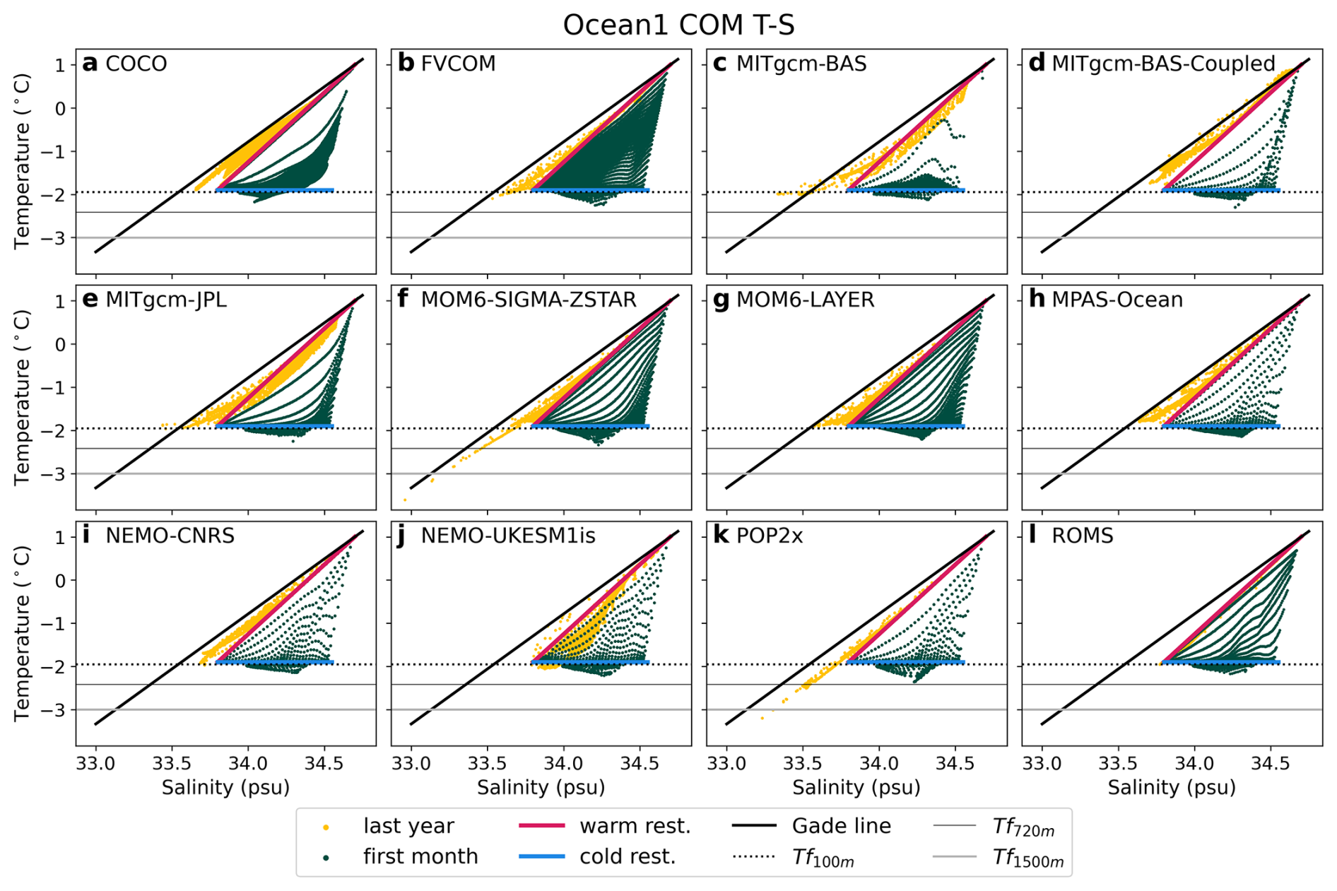
Figure 16 Temperature–salinity space verification of Ocean1 COM experiments. Model output averaged over the first month is shown in green, and averaged over the last year (year 20) in yellow. The warm and cold restoring profiles are shown by red and blue lines, respectively. The Gade line (see Eq. 6 for definition) is shown, indicating the meltwater mixing line in temperature–salinity space. Freezing points calculated from Eq. (2) are shown for three depths: 100, 720 (the maximum domain depth) and 1500 m. Ocean2 results are in Fig. S4.

To verify the simulated representation of ice–ocean thermodynamics in the models, we assess the water mass evolution in the warming Ocean1 experiment (Fig. 16). In the absence of other heat and freshwater sources, water mass properties should eventually be confined between the restoring conditions and the meltwater mixing line (Gade, 1979), along which a given water mass will cool and freshen at a constant ratio when interacting with the ice shelf at different depths. Neglecting heat conduction into the ice, as in the experimental protocol (Asay-Davis et al., 2016), the slope of these characteristic lines in temperature–salinity (T–S) space are given by

$$\begin{array}{}\text{(6)}& {\displaystyle \frac{\partial T}{\partial S}}={\displaystyle \frac{T_{\mathrm{w}}-T_{\mathrm{f}}+L/c_{\mathrm{w}}}{S_{\mathrm{0}}}},\end{array}$$

(Gade, 1979; Jenkins and Holland, 2007). Here, the specific heat capacity of seawater c_w and latent heat of fusion L are presented in Table 1. The salinity S₀ of the seawater in contact with the ice is taken as a constant S_ref=34.2 for simplicity, but with insignificant impact on the results. T_w is the temperature of the source water, taken to be the warmest water of the warm restoring condition, and T_f, the boundary layer freezing point, is taken to be the freezing point at the reference salinity and a depth of 360 m. Temperature and salinity data are taken from the cross-section of the model results at y=40 km, the most complete available datasets for this analysis. Fig. 16 shows that most models produce water masses within the expected range that is spanned by the restoring conditions and modification by ice shelf melting: T–S properties in all models deviate along the meltwater mixing line from the cold restoring properties (that were used as model initial conditions, blue line) to lower temperatures during the first month of the simulation, confirming the consumption of heat by basal melting of ice at greater pressure in the cold cavity. At the end of the simulation, this cold and saline water mass has been eroded by the warmer Ocean1 forcing, with most models featuring a T–S distribution in the last year (year 20, yellow colours) of the simulation that is bounded by the warm restoring conditions (red line), and the meltwater mixing line originating from the warmest water mass in the domain (black thick line), indicating mixing between these water masses. The absence of significantly colder temperatures than the 100 m melting point in most models at the end of the Ocean1 experiment is consistent with the paradigm of a warm ice shelf cavity circulation, where melt rates are limited by the fluxes across the ice-ocean boundary layer and a significant fraction of the available heat for melting is advected out of the cavity by the cavity circulation.

Some models show T–S properties at year 20 “to the right” of the warm restoring conditions (compare yellow and red colours in MITgm-BAS, MITgcm-JPL and NEMO-UKESM1is in Fig. 16). This feature could originate either from remnants of the initial conditions (unlikely, since models are well spun up; Fig. 12), or spurious salinification. The latter is known to have occurred in the imperfect application of the sea level restoring in NEMO-UKESM1is. Additionally, T–S properties “to the left” of the meltwater mixing line (MITgcm-BAS and MITgcm-JPL) indicate spurious freshwater. Both the spuriously fresh and saline features in these two models were found to be caused by the MITgcm advection scheme (https://mitgcm.readthedocs.io/en/latest/algorithm/adv-schemes.html, last access: 1 April 2026) used, the third-order DST flux limiter option 33 (and can be resolved with alternative advection schemes e.g. the second-order flux limiter option 77). Lower ocean temperatures than the freezing point at 720 m depth (the deepest ice in the domain) may indicate unphysical heat loss in two other models (POP2x and MOM6-SIGMA-ZSTAR, the latter found to be likely caused by diagnostic interpolation errors). T–S properties in ROMS lie below the warm restoring line, likely caused by a combination of the 5 m vertical resolution processed model output not capturing the cold, top boundary layer that is thinner than 5 m (the raw model data has water masses colder and fresher than the warm restoring line, not shown), and also that melting is driven by this cold boundary layer rather than warm restoring conditions, shifting the location of the Gade line. The latter highlights that differences in the water masses that drive melt (either through model differences, boundary layer and mixing choices) create different signatures in T–S space (Fig. 16).

For Ocean2, the water mass evolution reverses (Fig. S4), confirming a transition from a warm cavity into a cold cavity circulation paradigm. However, in some models (MITgcm-BAS-Coupled, MITgcm-JPL and NEMO-CNRS) there is less Ice Shelf Water (water masses colder than the surface freezing point, similar to the dotted line) present in the last year of the Ocean2 experiment compared to the first month of the Ocean1 experiment. These are the same models with a relatively warm interior in Fig. 3. The lack of Ice Shelf Water may be because these Ocean2 models have not yet reached their “cold” steady state (Figs. 3, 12) or a numerical issue, perhaps a consequence of the advection scheme issue noted in the Ocean1 analysis for the MITgcm models. The different ice base geometries between Ocean1 and Ocean2 may also affect the comparison between the first month of Ocean1 and last of Ocean2. The T–S space results indicate that water mass analysis is effective for model verification.

4.5 Typical experiment variability

The TYP set of experiments noted in Sect. 2.7 repeated the geometries and forcing used in Ocean1 and Ocean2 but allowed groups to configure their models as they would choose to do for a typical simulation, relaxing the stricter requirements of resolution, physics and parameter choices required for the COM experiments. COM simulations were the priority in ISOMIP+, and not all groups chose to conduct TYP simulations (Table 2). TYP configuration choices are described in Appendix A.

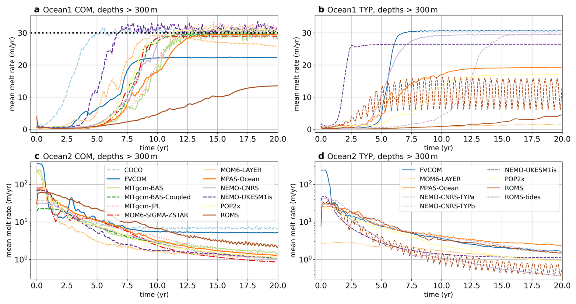
Figure 17 Time series of area-averaged melt rates at ice depths below 300 m for (a) Ocean1 COM, (b) Ocean1 TYP, (c) Ocean2 COM and (d) Ocean2 TYP ensembles.

There are a wide variety of differences between the COM and TYP configurations across the models so it is challenging to find simple explanations when comparing results between the two sets of experiments. It is generally true that a group's TYP model configuration produces less melt in response to the warm ocean forcing than using the idealised COM protocol (Fig. 17a, b), but this primarily reflects differences in resolution and parameterizations rather than the COM target melt rate being unrealistically high. Comparing melt below 300 m, which is the calibration depth used for setting each model's transfer coefficient values in Ocean0, the only model with a higher melt rate in its TYP configuration is FVCOM, which achieves this benchmark with the Ocean1 TYP configuration but not with COM, likely because of the use of different vertical mixing schemes. This lowering of melt rates and a marked increase in the variety of melt responses to warming suggests that the COM protocol was quite different to what model groups typically use, but succeeded in creating a common ground on which very different models could be compared. Although TYP models generally do not show more melt than COM, there is no consistent picture when comparing the rate at which the circulation spins up in the Ocean1 experiment. Temporal variability is similar in most TYP models compared to their Ocean1 COM counterparts, except for NEMO-UKESM1is, which has less temporal variability, and the ROMS model equipped with semidiurnal tides, which develops a clear periodic signal (likely showing resonance or aliasing in the monthly output).

There is less variation between COM and TYP in the Ocean2 experiment, with the models generally reducing their melt rates below 300 m at a similar rate (Fig. 17b, d). MPAS-Ocean has a higher final melt rate in TYP than COM in Ocean2 despite having a significantly lower melt rate in TYP compared to COM in Ocean1, and FVCOM shows the opposite behaviour, with more TYP melt in Ocean1 and less in Ocean2 compared to COM. This difference may be associated with changes in the depth at which the buoyant meltwater current separates from the ice. The two TYP variants of NEMO-CNRS achieve the same mean melt rate as each other in Ocean1 but with different timescales (possibly associated with different lateral momentum boundary conditions, vertical resolutions and melt distributions), and in Ocean2, after 20 years, they have spun down towards different area-average melt rates. As in COM, few of the Ocean2 TYP models have fully equilibrated melt rates at the end of the 20 years.

Even where TYP configurations produce similar melt rates to COM in response to the boundary forcing, similar melt rates can result from a different balance of physical processes (friction velocity and thermal driving) in the cavity (Fig. S7) and are also complicated by varying melt parameterisation choices. Generally, TYP models use smaller transfer coefficients than their COM counterparts (except for the NEMO simulations which tuned their melt rates to 30 m yr⁻¹, see Table 2 vs. Appendix. A4, A5), and are closer to those suggested by observations (e.g. $C_d^{\mathrm{1}/\mathrm{2}}{\mathrm{\Gamma }}_{\mathrm{T}}=\mathrm{1.1}\times {\mathrm{10}}^{-\mathrm{3}}$ suggested by Jenkins et al., 2010, in comparison to an average $C_d^{\mathrm{1}/\mathrm{2}}{\mathrm{\Gamma }}_{\mathrm{T}}$ of $\mathrm{3.0}\times {\mathrm{10}}^{-\mathrm{3}}$ across the COM models). However, note that transfer coefficients vary with ice shelf melt regimes and may not be constant in reality (Malyarenko et al., 2020; Rosevear et al., 2022). FVCOM TYP uses a smaller transfer coefficient than its COM counterpart but has a higher melt rate (Fig. 17b), likely explained by its more realistic vertical mixing scheme (Appendix A1), highlighting the importance of interior mixing choices on melt rates. Additionally, boundary layer temperature profiles of TYP configurations are also diverse and likely related to varying melt rate parameterisation and mixing choices (Figs. S9, S10).

In summary, the TYP experiments demonstrate how the COM experimental protocol moved many models away from their typical behaviour. There is significant variation in the simulated melt, melt drivers and circulation when models use their typical model parameters and resolution. However, untangling mechanisms and causes of model differences amongst the TYP models is challenging and emphasises the success of the COM experiments in providing a consistent common ground from which models can be compared.

5 Discussion

The ISOMIP+ project shows that there are a substantial number of ocean models now capable of simulating the ocean circulation in ice shelf cavities and its interactions with the ice shelf. These models have qualitatively similar hydrographic profiles, melt and circulation when forced with a common, idealised simulation protocol (“COM”). The twelve model configurations submitted to the common Ocean1 and Ocean2 experiments show similar temperature and salinity profiles consistent with the formation of a fresh, cold meltwater layer (Figs. 2, 3). Melt rates have similar spatial distributions, enhanced at the grounding line where thermal driving is greatest (Figs. 5, 6). All models reproduce the expected buoyancy-driven overturning circulation, and most have similar barotropic circulation within the ice shelf cavity (Figs. 8, 9, 10 11). Models also exhibit similarities during the spin-up, which occurs over a similar ∼ 5 year time period once initiated (Fig. 12). Melt and circulation strength are linearly proportional in a common relationship for most models, particularly for the Ocean1 experiment (Fig. 13). This common behaviour is not unsurprising given the prescribed, idealised model framework, but it is a positive outcome for the reliability of ice shelf cavity ocean models. Additionally, differences between the warm Ocean1 and cold Ocean2 experiments at steady state can be explained by the different forcing and ice base geometries.

However, there are differences between the models across several diagnostics. Melt rate patterns for Ocean1 vary (Figs. 5, 7), some affected by the vertical coordinate and modifications to geometry. Variation in melt rate spatial distributions, particularly near the grounding line and side walls, has implications for ice sheet evolution in coupled ocean–ice sheet models to be explored in the complementary MISOMIP1 model analysis (Hélène Seroussi and Nicolas Jourdain, personal communication, 2026). Overturning and barotropic streamfunctions also indicate differences in the cavity circulation patterns (Figs. 8–11). Both of these spatial distribution differences are likely to be at least partly associated with differences in bed topography and ice shelf draft as a result of model smoothing, particularly near side-walls, the grounding line and ice front, and vertical coordinate choices. Models also differ significantly in the ice–ocean boundary layer. ISOMIP+ COM models have their transfer coefficients tuned to achieve a given melt rate at depth, resulting in an order of magnitude spread of their values (Table 2). Boundary layer temperature and salinity (Figs. 14, S2), as well as thermal driving and friction velocity (Fig. 15), vary between models. These differences occur mainly between groups of models with different vertical coordinates, highlighting the sensitivity of ice shelf basal melt and circulation to the choice of the vertical coordinates (Gwyther et al., 2020) and emphasising the challenges in parameterising and modelling boundary layer processes under ice shelves in ocean models.

There are also outliers in certain diagnostics. The COCO setup used in ISOMIP+ has an anomalously strong circulation, possibly related to spurious currents from the implementation of the sponge boundary. The NEMO-UKESM1is setup used here has a known surface cooling error that results in a cooler interior. The MITgcm models used here have anomalously fresh meltwater associated with the advection scheme (Figs. 16, S4), and the transfer coefficients of MITgcm-BAS appear to be inconsistent (Fig. S3). POP2x and MOM6-SIGMA-ZSTAR displayed anomalously cold temperatures in the T–S diagrams, and the POP2x transfer coefficient was far larger than other z-coordinate models, indicating possible numerical issues. Many of these differences are likely associated with the imperfect implementation of the idealised model protocol rather than fundamental issues with the models. However, the ability to compare these models as part of the ISOMIP+ project allowed anomalous model behaviour to be identified, and in some cases, resolved. Outliers worth highlighting are the low melt rates in the ROMS and FVCOM model submissions (Fig. 12), which could not achieve the target melt rate of 30 m yr⁻¹ even with large transfer coefficients (Fig. 17a). The 30 m yr⁻¹ target was contrived based on a z-level model and may not represent what melt the Ocean0 domain and forcing would create in reality, particularly given the other idealised model assumptions made, such as the low internal vertical mixing and resolution – a limitation of the experimental setup. The ROMS and FVCOM results highlight the effect of different vertical coordinates, oceanic forcing sampling and flux distribution schemes on simulating ice shelf basal melting.

Low melt rates in ROMS and FVCOM can be explained by the high vertical resolution of their terrain-following coordinates, leading to relatively thin upper cell thicknesses. Meltwater fluxes are distributed into this upper cell and can only be mixed downwards by the explicit vertical mixing; most other models apply a Losch (2008)-style scheme, which induces an effective mixing over a chosen depth that is typically deeper than the s-coordinate top cell thickness. The paradigm used by ROMS and FVCOM thus likely leads to reduced vertical mixing of meltwater fluxes and a thin, fresh meltwater layer (Fig. 14), which is further emphasised by the prescribed low vertical mixing coefficients in the COM setup. Consequently, the sampling of temperature and salinity properties for the melt parameterisation will be more influenced by the colder meltwater fluxes leading to reduced thermal driving (Gwyther et al., 2020). Gwyther et al. (2020) demonstrate this effect using an ISOMIP+ Ocean0 experiment with a modified version of ROMS that effectively simulated a Losch (2008)-style scheme and find that melt rates increase with effective mixing depth (beyond 30 m yr⁻¹). Scott et al. (2023) also suggest that melt rates converge with higher vertical resolution and low vertical mixing. These studies suggest that models with higher resolution near the ice-ocean boundary, such as terrain-following and hybrid coordinate models, better represent the ice-ocean boundary layer with regard to numerical convergence (given a mixing and/or meltwater distribution scheme). At the same time, the results from the COM and TYP experiments highlight the sensitivity of the simulated melt rates and ice-ocean boundary layer structure to the integration of the applied basal melt parameterisation and the model's interior vertical mixing parameterisation, rather than indicating that the COM target melt rate itself was unrealistic.

The analysis of the TYP models (Sect. 4.5) highlights the variability in melt rates created by modifying model parameters. Since multiple changes may have been made between COM and TYP configurations, it is difficult to identify a causal link between specific parameter changes and the resultant ice shelf melt and circulation. However, it is clear that there is a complex relationship between melt rate, the spin-up of melt and circulation (Fig. 17), and melt rate drivers of friction velocity and thermal driving (Fig. S7), and that models typically used for realistic test cases vary significantly when compared in the ISOMIP+ idealised framework. Future work could more systematically probe causal links between model choices and consequent model solutions by performing parameter testing experiments or by tuning the TYP experiments to, for example, achieve a certain melt rate (as in COM; only the NEMO and FVCOM models used this approach in the TYP experiments presented here, Fig. 17). These experiments would test whether model states can be made more similar if their parameters have greater freedom to vary, noting that results likely still depend on the complexity of the model configuration used.

(Kusahara, 2025)(Zhou and Hattermann, 2025)(Hattermann and Zhou, 2025)(Jordan et al., 2025a)(Jordan et al., 2025b)(Nakayama, 2025)(Marques, 2025a)(Marques, 2025b)(Marques, 2025c)(Asay-Davis, 2025a)(Asay-Davis, 2025c)(Jourdain and Mathiot, 2025a)(Jourdain and Mathiot, 2025b)(Smith et al., 2025a)(Smith et al., 2025b)(Asay-Davis, 2025b)(Asay-Davis, 2025d)(Gwyther et al., 2025a)(Gwyther et al., 2025b)

Table 3 Digital Object Identifiers for ISOMIP+ model data registrations published on Open Science Framework.

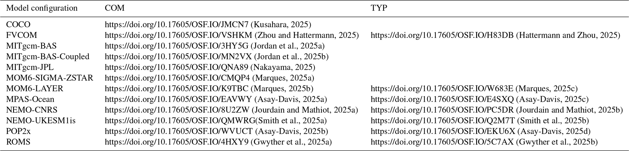
The variability seen in the ISOMIP+ ensemble may also be influenced by the model protocol. Models appear more similar in the original ISOMIP (Grosfeld et al., 1997; Losch, 2008; Holland et al., 2008; Galton-Fenzi, 2009; Gwyther et al., 2015, 2016; Mathiot et al., 2017), but this inter-model consistency largely reflects the simplicity of that configuration, which omits key processes relevant to Antarctic ice-shelf cavities (e.g. warm CDW inflow, thin turbulent boundary layers, complex topography). ISOMIP+ was designed to stress those processes, though still with a highly idealised geometry, and consequently highlights where models may differ: e.g. in the boundary layer, associated with vertical coordinates, or due to topography interpolation and smoothing differences at the boundaries amplified by the small domain. Other differences in ISOMIP+ may be exacerbated by the simplified forcing conditions: the open-ocean gyres that differ greatly between models are likely an artifact of the idealised, sponge-forced model setup that is highly sensitive to geometry choices (Zhao et al., 2022). The model variability in ISOMIP+ highlights that conclusions made with one idealised ocean model may not be directly applicable to other ocean models. This may be an important consideration for melt parameterisation development, particularly with machine learning methods. The results also demonstrate that the model representation of the ice shelf–ocean boundary layer is an area for future development.

Though there are clear differences between the ice shelf–ocean boundary layer and melt rates across models, there are already some methods to reconcile these. Different models may need different model parameters to achieve the same state, unlike the prescriptive COM protocol here. By calibrating the depth over which temperature, salinity and velocities are sampled in the three-equation melt parameterisation and the distance over which freshwater or a virtual salt flux is distributed, similar melt rates can be achieved with different vertical coordinates and resolution (Gwyther et al., 2020). Melt rates can also converge as the vertical resolution is enhanced (Scott et al., 2023). Models will likely require tuning and development of new melt parameterisations in future Antarctic ice shelf simulations, in both idealised and realistic configurations, to achieve melt rates and ice shelf cavity conditions consistent with in situ observations. Tidal forcing is also an important process that is missing from ISOMIP+ (with the exception of the ROMS TYP submission) and will affect ice shelf melt. The integration of melt parameterisations with the model-specific interior vertical mixing schemes, which may depend on vertical coordinates, is also an area for future work.

When simulating realistic geographic domains, model choices are expected to also play a large role between models (Naughten et al., 2018b; Richter et al., 2022; Galton-Fenzi et al., 2025b). However, ocean models may be constrained to prescribed atmospheric forcings or tuned to achieve an ocean and ice state similar to existing observations, using greater parameter freedom than in ISOMIP+. Realistic ice shelf–ocean model intercomparison projects such as RISE (Galton-Fenzi et al., 2025b) and MISOMIP2 (De Rydt et al., 2024) are therefore able to validate models and assess biases compared to limited observations, something ISOMIP+ cannot do. These realistic projects will provide the next assessments of our ice sheet-ocean modelling capabilities and guide future model development. As has been done in the past, this model development will likely rely on idealised models of varying complexity: highly idealised for verification, and adding complexity for benchmarking. For example, the next generation of idealised ice shelf–ocean models might consider including features not included in ISOMIP+, such as rough topography, eddies, tides and more realistic ice shelf cavity stratification, and learn from the difficulties of the ISOMIP+ sponge boundary. They may also consider a higher vertical resolution to better resolve the ice shelf–ocean boundary layer. In lieu of observations or an analytical solution in idealised models, the latter of which is an area for future work, attempting to achieve model solution convergence with increased resolutions may better establish a truth for benchmarking of these models. Going forward, we see idealised and realistic experiments as complementary, and expect the community will continue to oscillate between the two in order to both understand mechanisms and test against observations, as we work towards improved ice shelf–ocean model fidelity.

6 Conclusions

We have presented the results of the second Ice Shelf–Ocean Model Intercomparison Project, ISOMIP+. Twelve model configurations (eight independent ocean models) in a common model setup were submitted across a tuning and two forcing experiments. Nine model configurations were also submitted in a more flexible, typical category. Through the common, idealised modelling framework, we demonstrate the consistency in simulated basal melt rate and ice shelf cavity circulation across the models and a shared relationship between melt rate and circulation. However, we highlight the differences in boundary layer characteristics between models and the order of magnitude spread in transfer coefficients required to parameterise a common melt rate. We find that many differences in the model results can be explained by the use of different vertical coordinates. This sensitivity highlights the need for improved model representation of ice-shelf boundary layers and the physical processes within, and their integration with the model-specific interior vertical mixing schemes, requiring further research and direct observations of the boundary layer. When constraints on model parameters are relaxed, the variation in boundary layers, melt rate and cavity circulation is further enhanced. However, this variation may be enhanced by the idealised nature of the ISOMIP+ setup, where not all the models could follow the exact idealised protocol. Future work will compare models in realistic ice shelf–ocean configurations to assess the state of ice sheet–ocean modelling and guide model development for improved Antarctic Ice Sheet, climate and sea level projections.

Appendix A: Typical model configurations (TYP)

Here, we outline the changes made to develop the TYP configurations from the COM experiments for each model. Where details are missing, models use the COM parameters (Sect. 3).

A1 FVCOM

The horizontal resolution in the FVCOM TYP submission is increased in regions of steeply sloping bed topography and ice shelf draft (ranging from 200–2000 m). Mixing schemes that are typically used in more realistic applications were also employed. Vertical mixing uses the Mellor and Yamada level 2.5 turbulent closure model (Mellor and Yamada, 1982; Galperin et al., 1988) with background viscosity and diffusivity set to 10⁻⁵ m² s⁻¹. Horizontal mixing uses the Smagorinsky eddy parameterisation (Smagorinsky, 1963), with the constant used in the parameterisation being 0.1. Alternative transfer coefficients of Γ_T=0.06 and ${\mathrm{\Gamma }}_{\mathrm{S}}=\mathrm{1.7}\times {\mathrm{10}}^{-\mathrm{3}}$ are also used.

A2 MOM6-LAYER

The MOM6-LAYER TYP submission is similar to MOM6-LAYER COM, but has a higher vertical resolution with 72 isopycnal layers. The ice geometry is also modified to have a minimum ocean thickness of 40 m. The Holland and Jenkins (1999) basal melt parameterisation is used with the McPhee (1981) stability parameter. The experiments also included frazil ice formation, in which seawater is artificially warmed to its freezing point when the temperature falls below that threshold.

A3 MPAS-Ocean

The MPAS-Ocean TYP submission has a coarser horizontal resolution than COM, of 5 km, which is close to the highest resolution that MPAS-Ocean is typically run at in the Energy Exascale Earth System Model (E3SM). Horizontal momentum is mixed with a biharmonic scheme, with ${\mathit{\nu }}_{\mathrm{H}}=-\mathrm{1.0}\times {\mathrm{10}}^{\mathrm{9}}{\mathrm{m}}^{\mathrm{4}}{\mathrm{s}}^{-\mathrm{1}}$, and tracers were not mixed horizontally. Vertical mixing is parameterised by the Community Vertical Mixing library (CVMix Griffies et al., 2015) with background vertical diffusion and shear-based mixing via the K-Profile Parameterization (Large et al., 1994) (parameter values in supplementary model description documents). Output is presented as snapshots rather than monthly output due to constraints at the time of production. A nonlinear density equation of state from Jackett and Mcdougall (1995) is used, and a nonlinear freezing equation of state (a least-squares fit to TEOS-10, Millero et al., 2008, over salinities between 20 and 40 and pressures between 0 and 2×10⁷ Pa) is also used with a salinity–pressure cross-term (${\mathit{\lambda }}_{\mathrm{1}}=-\mathrm{5.64}\times {\mathrm{10}}^{-\mathrm{2}}\mathit{°}\mathrm{C}$, ${\mathit{\lambda }}_{\mathrm{2}}=\mathrm{6.22}\times {\mathrm{10}}^{-\mathrm{2}}\mathit{°}\mathrm{C}$, ${\mathit{\lambda }}_{\mathrm{3}}=-\mathrm{7.43}\times {\mathrm{10}}^{-\mathrm{8}}\mathit{°}\mathrm{C}{\mathrm{Pa}}^{-\mathrm{1}}$, ${\mathit{\lambda }}_{\mathrm{4}}=-\mathrm{1.74}\times {\mathrm{10}}^{-\mathrm{10}}\mathit{°}\mathrm{C}{\mathrm{Pa}}^{-\mathrm{1}}$). The transfer coefficients from Jenkins et al. (2010) were used; Γ_T=0.011 and ${\mathrm{\Gamma }}_{\mathrm{S}}=\mathrm{3.1}\times {\mathrm{10}}^{-\mathrm{4}}$. The tidal velocity is increased to 0.05 m s⁻¹ and bottom drag coefficient decreased to $\mathrm{1}\times {\mathrm{10}}^{-\mathrm{3}}$.

A4 NEMO-CNRS

There are two NEMO-CNRS submissions, TYPa and TYPb.

TYPa has a 2.4 km resolution and 75 vertical levels ranging from 1 m at the surface to ∼ 100 at 1000 m depth. This grid represents the $\mathrm{1}/\mathrm{12}$° NEMO configuration used for the Amundsen Sea in Jourdain et al. (2017). Compared to the NEMO-CNRS COM configuration, TYPa uses the EOS80 equation of state (ICES, SCOR, and IAPSO, 1981), a 100 times stronger vertical mixing in unstable conditions, a TKE vertical mixing scheme in stable conditions (Madec et al., 2019), a 30 m Losch (2008)-style layer over which temperatures, salinities and velocities are averaged to compute melt, and lateral advection and diffusion as in Jourdain et al. (2017), with partial slip as lateral boundary condition for momentum. The prescribed tidal velocity is set to zero. The transfer coefficients are modified to ${\mathrm{\Gamma }}_{\mathrm{T}}=\mathrm{4.8}\times {\mathrm{10}}^{-\mathrm{2}}$ and ${\mathrm{\Gamma }}_{\mathrm{S}}=\mathrm{1.37143}\times {\mathrm{10}}^{-\mathrm{3}}$, while the top interface drag coefficient is $C_{\mathrm{D}}=\mathrm{1.0}\times {\mathrm{10}}^{-\mathrm{3}}$.

TYPb is a more idealised experiment, similar to the COM experiment, but run at 1 km resolution and with a different representation of vertical mixing: the TKE scheme in stable conditions and a 100 times stronger vertical mixing in unstable conditions. The Losch (2008)-style layer over which temperatures, salinities and velocities are averaged to compute melt is also thinner, with 10 m thickness. Although not identical, this experiment is similar to the TYP-1km experiment described in Favier et al. (2019). Transfer coefficients are modified to ${\mathrm{\Gamma }}_{\mathrm{T}}=\mathrm{2.63}\times {\mathrm{10}}^{-\mathrm{2}}$ and ${\mathrm{\Gamma }}_{\mathrm{S}}=\mathrm{7.51429}\times {\mathrm{10}}^{-\mathrm{4}}$.

A5 NEMO-UKESM1is

The NEMO-UKESM1is TYP setup is very similar to UKESMis simulation (Smith et al., 2021). The major difference with COM is the use of a coarse grid equivalent to a sector of the eORCA025 global grid used in GO7 (Storkey et al., 2018). Horizontal diffusivity of momentum is biharmonic and along geopotentials, horizontal tracer diffusivity is increased to ${\mathit{\kappa }}_{\mathrm{H}}=\mathrm{260}{\mathrm{m}}^{\mathrm{2}}{\mathrm{s}}^{-\mathrm{1}}$, a weaker vertical stable mixing is used (${\mathit{\nu }}_{\mathrm{stab}}=\mathrm{1}\times {\mathrm{10}}^{-\mathrm{4}}{\mathrm{m}}^{\mathrm{2}}{\mathrm{s}}^{-\mathrm{1}}$, ${\mathit{\kappa }}_{\mathrm{stab}}=\mathrm{1}\times {\mathrm{10}}^{-\mathrm{5}}{\mathrm{m}}^{\mathrm{2}}{\mathrm{s}}^{-\mathrm{1}}$), a 100 times stronger vertical mixing (${\mathit{\kappa }}_{\mathrm{unstab}}=\mathrm{10}{\mathrm{m}}^{\mathrm{2}}{\mathrm{s}}^{-\mathrm{1}}$) is used in unstable conditions, the convective vertical viscosity ν_stab is set to zero, and the TEOS-10 equation of state (IOC et al., 2010; Roquet et al., 2015) is used. The lower bottom drag coefficient is decreased to $\mathrm{1.0}\times {\mathrm{10}}^{-\mathrm{3}}$, and a diffusive bottom boundary layer parameterisation is used. As in COM, the evaporative flux that maintains sea level was incorrectly allowed to affect the salinity of the remaining surface water. The Γ_T and Γ_S coefficients were tuned to achieve the COM target melt rate in Ocean0, and are Γ_T=0.06, Γ_S=0.001714.

A6 POP2x

The POP2x TYP submission has a different model resolution compared to its COM counterpart of 4 km in the horizontal and 48 layers in the vertical, with increasing thickness with depth from 10 m at the surface to 40 m at the bottom. A thicker layer of 30 m is used to sample temperature and salinity for the melt parameterisation as well as distribute the melt fluxes, and the transfer and drag coefficients from Jenkins et al. (2010), Γ_T=0.011, ${\mathrm{\Gamma }}_{\mathrm{S}}=\mathrm{3.1}\times {\mathrm{10}}^{-\mathrm{4}}$ and $C_{\mathrm{D},\mathrm{top}}=\mathrm{9.7}\times {\mathrm{10}}^{-\mathrm{3}}$ were used, with bottom drag reduced to $C_{\mathrm{D},\mathrm{bottom}}=\mathrm{1}\times {\mathrm{10}}^{-\mathrm{3}}$. The configuration uses a nonlinear density equation of state from McDougall et al. (2003) and a modified linear freezing equation of state (${\mathit{\lambda }}_{\mathrm{1}}=-\mathrm{5.89}\times {\mathrm{10}}^{-\mathrm{2}}\mathit{°}\mathrm{C}$, λ₂=0.153°C, ${\mathit{\lambda }}_{\mathrm{3}}=-\mathrm{8.04}\times {\mathrm{10}}^{-\mathrm{8}}\mathit{°}\mathrm{C}{\mathrm{Pa}}^{-\mathrm{1}}$). Vertical mixing is parameterised with the Pacanowski and Philander (1981) convective adjustment scheme based on the Richardson number with ${\mathit{\nu }}_b=\mathrm{1}\times {\mathrm{10}}^{-\mathrm{3}}{\mathrm{m}}^{\mathrm{2}}{\mathrm{s}}^{-\mathrm{1}}$, ${\mathit{\kappa }}_b=\mathrm{1}\times {\mathrm{10}}^{-\mathrm{4}}{\mathrm{m}}^{\mathrm{2}}{\mathrm{s}}^{-\mathrm{1}}$ and ${\mathit{\nu }}_{\mathrm{0}}=\mathrm{5}\times {\mathrm{10}}^{-\mathrm{3}}{\mathrm{m}}^{\mathrm{2}}{\mathrm{s}}^{-\mathrm{1}}$. The unstable enhanced vertical mixing is increased ten-fold to 1 m² s⁻¹. Biharmonic horizontal mixing is used with ${\mathit{\nu }}_{\mathrm{H}}=-\mathrm{7.0}\times {\mathrm{10}}^{\mathrm{9}}{\mathrm{m}}^{\mathrm{4}}{\mathrm{s}}^{-\mathrm{1}}$. The tidal velocity is increased to 0.05 m s⁻¹.

A7 ROMS

The two ROMS TYP configurations use different mixing schemes to COM. Vertical diffusivity and viscosity is implemented through the K-Profile Parameterisation (KPP, Large et al., 1994) with parameters ${\mathit{\nu }}_{\mathrm{stab}}=\mathrm{1}\times {\mathrm{10}}^{-\mathrm{4}}{\mathrm{m}}^{\mathrm{2}}{\mathrm{s}}^{-\mathrm{1}}$ and ${\mathit{\kappa }}_{\mathrm{stab}}=\mathrm{1}\times {\mathrm{10}}^{-\mathrm{6}}{\mathrm{m}}^{\mathrm{2}}{\mathrm{s}}^{-\mathrm{1}}$ and unstable mixing coefficients are calculated by KPP. Horizontal harmonic diffusion for tracers is set to zero. Horizontal mixing of momentum and tracers are both scaled by grid size, and momentum diffusion is computed along sigma surfaces rather than geopotential levels. A nonlinear density equation of state is used (Jackett and Mcdougall, 1995), with coefficients available in the model description PDF. Turbulent exchange velocities follow McPhee et al. (1987) rather than constant transfer coefficients. The linear freezing equation of state is also modified slightly (${\mathit{\lambda }}_{\mathrm{1}}=-\mathrm{5.7}\times {\mathrm{10}}^{-\mathrm{2}}\mathit{°}\mathrm{C}$, ${\mathit{\lambda }}_{\mathrm{2}}=-\mathrm{0.0939}\times {\mathrm{10}}^{-\mathrm{2}}\mathit{°}\mathrm{C}$, ${\mathit{\lambda }}_{\mathrm{3}}=-\mathrm{7.61}\times {\mathrm{10}}^{-\mathrm{4}}\mathit{°}{\mathrm{Cm}}^{-\mathrm{1}}$). The ROMS tides run also includes a forced tide with a 12 h period, designed to emulate the S2 tide. This is achieved by forcing the u-momentum at the x=800 km boundary towards a barotropic sinusoidal profile with 0.5 m s⁻¹ amplitude.