Southwest Greenland supraglacial lake bathymetry derived from ICESat-2 and spectral stratification of satellite imagery

Arctic supraglacial lakes volume changes serve as critical indicators of global temperature fluctuations. Accurate lake depth measurements are essential for reliable volume estimation, yet traditional bathymetry methods (e.g., airborne LiDAR and shipborne sonar) face significant challenges and high costs in the harsh Arctic environment, and are also inadequate for capturing the rapid temporal variability in lake depth. To address this, we utilized satellite-derived bathymetry (SDB) to achieve supraglacial lake water depth inversion. Specifically, three approaches were tested: (i) applying the radiative transfer equation (RTE) model (Philpot RTE model) using only Sentinel-2 multispectral optical imagery; (ii) combining ICESat-2 (Ice, Cloud, and Land Elevation Satellite-2) single photon-counting laser altimetry data with Sentinel-2 imagery through a semi-empirical log-transformed linear regression model (Lyzenga model); and (iii) a proposed novel approach that optimizes the model by considering the varying reflectance characteristics across different spectral bands in the water column. For the proposed method, we propose an SDB approach based on spectral stratification using the Otsu algorithm (maximum between-class variance method), and further integrate the spectral stratification with the Lyzenga model. To validate the effectiveness of the proposed method, we applied it to four relatively large and morphologically intact lakes on the southwest Greenland Ice Sheet (GrIS), using time-stamped ArcticDEM (Arctic Digital Elevation Model) strips as reference data. Compared with the Philpot RTE model, the root mean square error (RMSE) and mean absolute error (MAE) were reduced by up to 86.6 % and 89.0 %, respectively; compared with the traditional Lyzenga model, the RMSE and MAE decreased by up to 13.0 % and 14.0 %, respectively. The enhanced accuracy of our approach improves the ability to monitor volume changes in GrIS supraglacial lakes, providing valuable insights into their response to environmental changes.

1 Introduction

The Arctic plays a crucial role in maintaining Earth's temperature balance and exhibits heightened sensitivity to global climate change (Box et al., 2019; Sand et al., 2016; Schmale et al., 2021). The accelerated melting of Arctic glaciers in recent years, driven by global warming, has exerted substantial negative impacts on the global ecological environment (Beckmann and Winkelmann, 2023; Box et al., 2022). Greenland Supraglacial Lakes (SGLs) are formed in depressions on the surface of the Greenland Ice Sheet (GrIS). Their volume is influenced by factors such as runoff (meltwater, rain, and refreezing) and lake drainage (Leeson et al., 2015). These changes in water volume within Arctic SGLs are closely linked to ice sheet dynamics through a critical mechanism: when lake depth and volume reach sufficient thresholds, rapid drainage events can deliver massive amounts of meltwater to the glacier bed, triggering basal lubrication and ice acceleration (Das et al., 2008; Stevens et al., 2015). Observations demonstrate this volume-dependent control on glacier dynamics: a drainage event at Store Glacier transferred 4.8 million m³ of water to the bed within 5 h, accelerating ice flow from 2.0 to 5.3 m d⁻¹ (Chudley et al., 2019), while cascading drainage across lake networks has produced 50 %–100 % velocity increases over distances exceeding 80 km (Christoffersen et al., 2018). Therefore, accurate quantification of lake depth and volume is essential for understanding ice sheet response to climate warming and predicting future sea level contributions.

Accurately estimating the volume of these lakes requires detailed bathymetry data, which is particularly challenging to obtain due to the harsh climatic conditions in the Arctic. Although conventional bathymetric methods, including bathymetric airborne LiDAR and shipborne sonar, have achieved high levels of maturity and accuracy, and also been successfully applied over the GrIS (Box and Ski, 2007; Tedesco and Steiner, 2011); due to limitations in cost and timeliness (Li et al., 2022; Qi et al., 2022, 2024), these methods cannot meet the monitoring demands of rapidly changing SGLs on GrIS. This limitation restricts the acquisition of continuous spatiotemporal volume data for SGLs. With advancements in satellite remote sensing technology, satellite-derived bathymetry (SDB) has emerged as a promising method for estimating bathymetry in clear water areas using multispectral imagery (Ma et al., 2020). Classic bathymetry inversion models, such as the log-transformation linear regression model (Lyzenga model) and the log-transformation ratio model (Stumpf model) (Lyzenga, 1978, 1985; Stumpf et al., 2003), are widely used in water depth inversion, but their accuracy is constrained by the lack of in-situ depth data.

In recent years, the launch of the spaceborne single-photon altimetry satellite ICESat-2 (Ice, Cloud, and Land Elevation Satellite-2) has partially mitigated challenges in obtaining precise water depth measurement data (Albright and Glennie, 2020; Li et al., 2023). Numerous studies have integrated multispectral imagery with ICESat-2 to conduct bathymetric detection and inversion, leveraging both passive and active remote sensing methods. These studies have yielded significant results, primarily in island reef areas. Cao et al. (2016) developed a high-precision bathymetry model for Ganquan Island in the South China Sea by using laser satellite data and optical imagery. This approach leverages active and passive remote sensing techniques, tailored to the specific characteristics and requirements of shallow water bathymetry. Ma et al. (2020) used ICESat-2 data and Sentinel-2 data to retrieve the bathymetry information of the Xisha Islands and Aklin Island. Chu et al. (2023) considered the penetration limit bathymetry in different bands of multispectral imagery and proposed an SDB method based on spectral stratification, which was successfully applied to the long line reefs in the Nansha area of China and Buck Island in the United States Virgin Islands, improving the inversion accuracy to a certain extent. For the bathymetry inversion in polar lakes, Lin et al. (2012) used multibeam bathymetric data and Landsat TM data to invert the bathymetry of lakes in the Arctic Alaska Coastal Plain. Pope et al. (2016) also utilized the Landsat satellites with the OLI sensor, applying both the Philpot radiative transfer equation (RTE) model (Philpot, 1987) and a semi-empirical model based on partial in situ measurements to estimate the water volume of SGLs in western GrIS. The results were evaluated and validated using satellite stereo-derived elevation data. Similarly, Moussavi et al. (2016) also utilized the stereoscopic imaging capability of Worldview-2 data to estimate and validate the bathymetry of SGLs on the GrIS, achieving high accuracy. Williamson et al. (2018) applied this RTE approach to Sentinel-2 multispectral imagery. Through the synergistic use of Sentinel-2 and Landsat 8 satellites, they identified numerous drained lakes, providing algorithmic support for water depth and volume estimation. Melling et al. (2024) used Sentinel-2 data to construct the Philpot RTE for different bands and validated them with ICESat-2 and ArcticDEM (Arctic Digital Elevation Model) data. Based on a rigorous adherence to physical principles, they evaluated the applicability of the RTE model to SGLs. Fricker et al. (2021) utilized ICESat-2 data to estimate the meltwater depth of the Antarctic ice sheet (AIS) and GrIS, providing a reference for the AIS and GrIS SGLs water depth inversion. Datta and Wouters (2021) proposed the Watta algorithm, which automatically calculates SGLs bathymetry and detects potential ice layers along tracks of the ICESat-2, focusing on the drainage situation of arctic lakes by utilizing ICESat-2 data and multispectral data. Lv et al. (2024) used the Stumpf model, combined with ICESat-2 and Sentinel-2 imagery, to invert the bathymetry of some SGLs on the GrIS from 2019 to 2023. Lutz et al. (2024) integrated ICESat-2 altimetry, in situ sonar measurements, and the RTE to establish four depth estimation methods, validated against TanDEM-X elevation models, providing a systematic methodological comparison for supraglacial lake depth and volume estimation in GrIS. Feng et al. (2025) integrated ICESat-2 and Sentinel-2 data using a multi-layer perceptron neural network for depth inversion, achieving volumetric evolution monitoring of SGLs throughout the 2022 melt season in southwestern GrIS.In this study, we further extend previous methods for retrieving SGLs bathymetry. Inspired by Chu et al. (2023) on offshore islands and reefs, we applied an improved bathymetric inversion approach for SGLs that combines active and passive remote sensing. Specifically, ICESat-2 LiDAR data were integrated with Sentinel-2 multispectral imagery, taking into account the varying penetration abilities of different spectral bands (i.e., red, green, blue, and near-infrared). The Sentinel-2 imagery was divided into multiple spectral layers using the Otsu algorithm to construct a spectral stratification-based Lyzenga model. In this framework, ICESat-2 lake bottom photons were used as training samples to build semi-empirical models for each spectral layer, thereby improving the accuracy of SGLs bathymetric estimation. For comparison, we also applied the Philpot RTE model and traditional Lyzenga model without spectral stratification to the same study area. All results were validated against high-resolution ArcticDEM data. This study provides a new and more accurate approach for monitoring the volumes of SGLs and offers methodological guidance for SGL bathymetry research.

2 Study area and data

2.1 Study area

The study area is located in the southwest of the GrIS. This region contains numerous shallow SGLs with clear water, providing good conditions for bathymetry retrieval using ICESat-2 laser altimetry and multispectral remote sensing imagery (Feng et al., 2025). Four SGLs are selected for research and analysis, as depicted in Fig. 1. For convenience, these lakes are referred to as Lake A, Lake B, Lake C, and Lake D. The study aims to validate the feasibility of the bathymetric inversion model using these four lakes. Subsequently, the bathymetry data obtained by the proposed method were used to calculate the volume information of these four lakes.

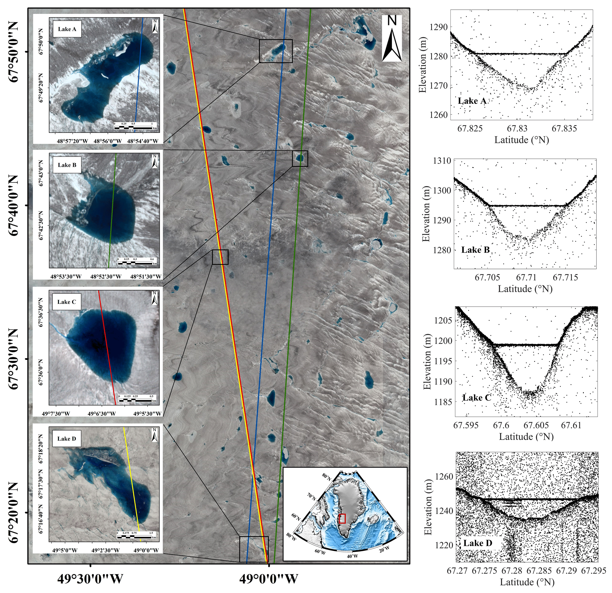
Figure 1 Overview of the study area and typical lakes. The background consists of Sentinel-2 multispectral imagery depicting the study area and the four lakes. Blue, green, red, and yellow lines represent ICESat-2 tracks traversing these four lakes, respectively. The black points indicate ICESat-2 raw photon data.

2.2 Study data

2.2.1 Sentinel-2 optical multispectral imagery

The Sentinel-2 satellite, a medium-resolution multispectral satellite launched by the European Space Agency (ESA), is a critical component of its Earth observation mission. The Sentinel-2 system comprises three satellites (i.e., Sentinel-2A, Sentinel-2B, and Sentinel-2C), which were launched on 23 June 2015, 7 March 2017, and 5 September 2024, respectively. The Sentinel-2 satellite features 13 bands covering visible light, near-infrared, and shortwave infrared bands, with some bands having a resolution of up to 10 m (Hedley et al., 2018). Sentinel-2 imagery spans a width of up to 290 km and a single satellite revisit period of 10 d. In this study, the detailed information of Sentinel-2 data used in this study is listed in Table 1. The Sentinel-2 multispectral imagery data were downloaded for free from Copernicus Open Access Hub (https://dataspace.copernicus.eu/data-collections/copernicus-sentinel-missions/sentinel-2, last access: 27 January 2026).

2.2.2 ICESat-2 single-photon LiDAR data

The ICESat-2 satellite orbits at an altitude of approximately 500 km with an inclination of 92°, observing the Earth's surface between latitudes 88° S and 88° N. The platform is equipped with the Advanced Topographic Laser Altimeter System (ATLAS) single-photon LiDAR and auxiliary system, which determines the distance between the spacecraft and the Earth's surface by measuring the round-trip time of photons (Markus et al., 2017). The ICESat-2/ATLAS laser emits laser pulses with a wavelength of 532 nm and a width of 1.5 ns at a frequency of 10 kHz, forming overlapping light spots along the Earth's surface with a laser footprint spacing of approximately 0.7 m (Magruder et al., 2021). The left and right points of each beam pair are approximately 90 m apart in the cross-track direction and approximately 2.5 km apart in the along-track direction. Paired tracks are approximately 3.3 km apart in the transverse track direction (Neumann et al., 2021). The detailed information of ICESat-2 used in this study is listed in Table 1. The ICESat-2 data can be obtained freely from NASA Earthdata (https://search.earthdata.nasa.gov/, last access: 27 January 2026). Due to the rapid morphological changes of SGLs, ICESat-2 data were selected as close as possible in time to Sentinel-2 imagery. This study utilized ICESat-2 data intercepted from Sentinel-2 data as training data, and assumed a lake water depth of 0 m at the edges of the ICESat-2 tracks.

2.2.3 ArcticDEM data

ArcticDEM data were obtained for free from the Polar Geospatial Center at the University of Minnesota in the United States (https://www.pgc.umn.edu/data/arcticdem/, last access: 28 April 2025). It is primarily generated using satellite stereophotogrammetry, covering all land areas above 60° north latitude, with a spatial resolution of up to 2 m, and has significant reference value for topographic research in the Arctic region (Porter et al., 2022). The data is extracted and output as strip-shaped DEM data by SETSM (Surface Extraction with TIN-based Search space Minimization), preserving the time information of the original data and allowing users to service data for research and analysis as needed (Morin et al., 2016). In this study, the most recent version (s2s041) of ArcticDEM strips were used to validate the accuracy of the bathymetry and volume estimated results. Due to the sparse temporal sampling of ArcticDEM, the validation data used in this study differ from the ICESat-2 and Sentinel-2 observations by several months. The GrIS is covered by ice, and both the ice surface and supraglacial lakes evolve, making short-term morphological changes unavoidable. However, as noted by Echelmeyer et al. (1991), many large supraglacial lakes remain fixed in space because their surface depressions are dynamically supported by irregularities in the underlying bedrock. This bedrock control limits large-scale spatial shifts within short periods, although minor variations are inevitable. Consequently, some discrepancies between ICESat-2-derived bathymetry and ArcticDEM data collected several months apart are expected. Nevertheless, the overall consistency between the two datasets remains strong, as also demonstrated in the experiment by Melling et al. (2024). These differences fall within an acceptable range and do not compromise the reliability of ArcticDEM as a high-quality reference dataset. The detail information of ArcticDEM data used in this study is listed in Table 1.

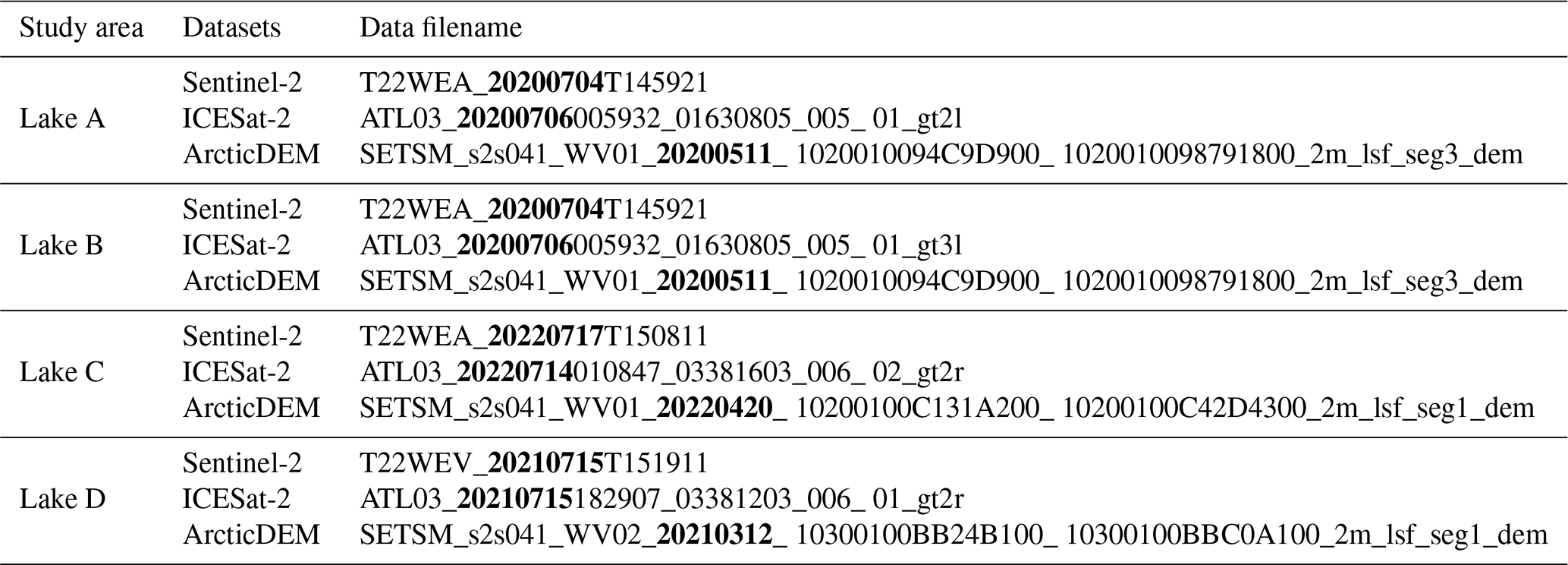
Table 1 Detailed information of the datasets used in this study, the acquisition dates are highlighted in bold within the dataset names in the format yyyy/mm/dd.

3 Methodology

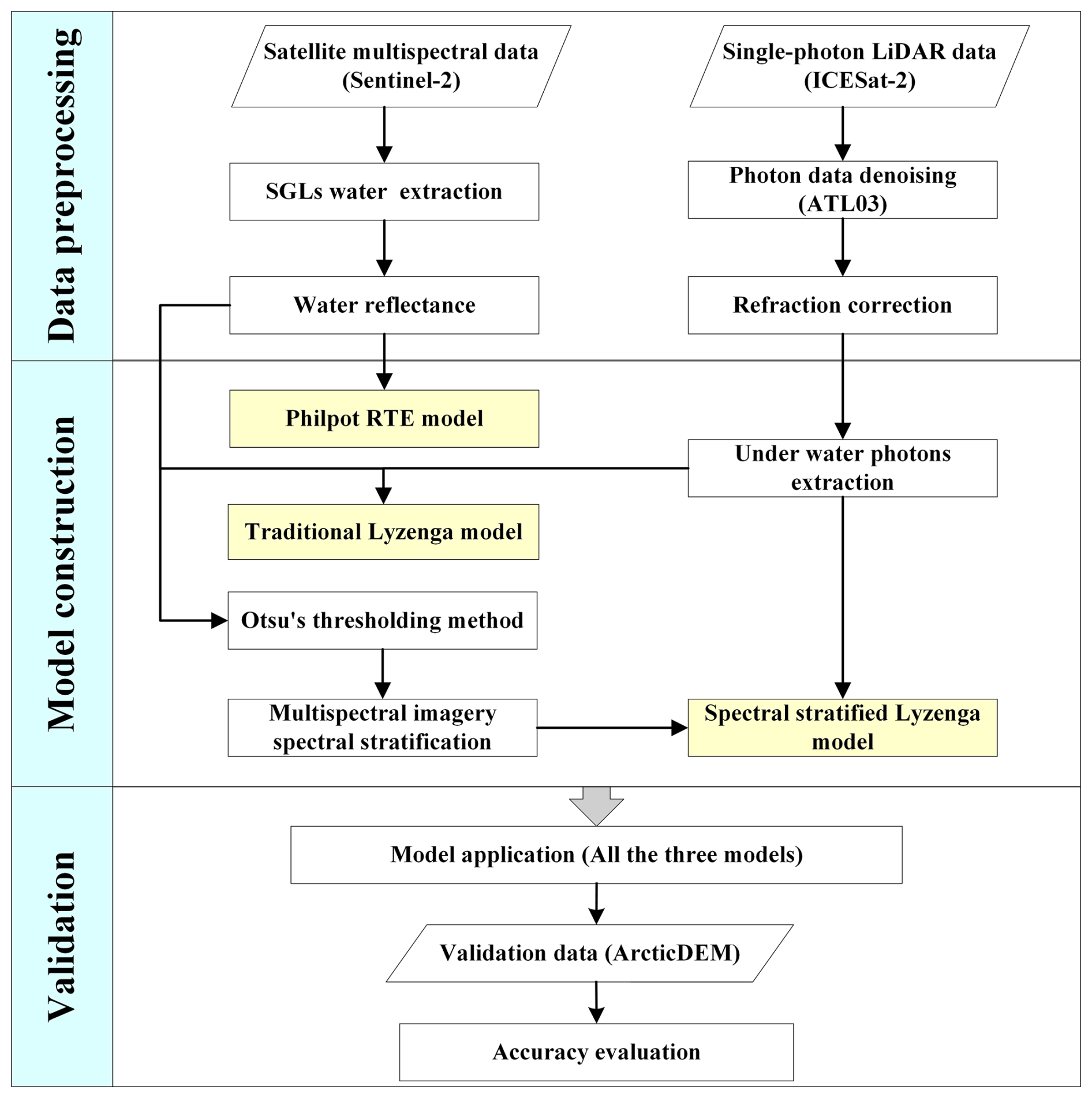
To improve the accuracy of SDB for SGLs of GrIS, this study compares three approaches: the physically-based RTE model proposed by Philpot in 1987, the traditional Lyzenga model, and a novel spectrally stratified optimized Lyzenga model. While the RTE model relies on physical parameterization of water column properties, and the traditional Lyzenga model combines multiple spectral bands empirically, while these approaches incorporate spectral information through wavelength-dependent attenuation coefficients, they generally do not stratify the retrieval model based on the varying effective depth ranges of different spectral bands. Inspired by the spectral stratification method applied to shallow coral reefs by Chu et al. (2023), this study adapts and extends this approach to SGLs. The proposed method combines ICESat-2 data with Sentinel-2 multispectral imagery. Using the Otsu algorithm (Otsu, 1979), spectral stratification is performed based on radiance differences at various water depths across different bands. The stratified spectral layers are then combined with ICESat-2 bathymetric data to construct optimized Lyzenga models for each spectral layer. The detailed workflow is illustrated in Fig. 2.

Figure 2 Workflow for the three bathymetry methods.

3.1 Data processing

3.1.1 Pre-processing of multispectral imagery

The Sentinel-2 data are divided into Level-1C (L1C) and Level-2A (L2A) products. L1C products are ortho-rectified top-of-atmosphere (TOA) reflectance products; L2A products are atmospherically-corrected bottom-of-atmosphere (BOA) reflectance products. This study used the L2A products for research analysis. The water column was extracted from multispectral imagery using water-land separation methods, i.e., the Normalized Difference Water Index (NDWI), specifically its variant adapted for water extraction in ice–snow covered environments (Eq. 1) (McFeeters, 1996; Yang and Smith, 2012), combined with threshold-based grayscale segmentation.

$$\begin{array}{}\text{(1)}& {\mathrm{NDWI}}_{\mathrm{Ice}}={\displaystyle \frac{\mathrm{Blue}-\mathrm{Red}}{\mathrm{Blue}+\mathrm{Red}}}\end{array}$$

where Blue represents the reflectance at the blue band (corresponding to Sentinel-2 Band 2), and Red represents the reflectance at the red band (corresponding to Sentinel-2 Band 4).

The image was divided into water and non-water parts using the NDWI_Ice, with the non-water portion – including lake ice – applied as a mask to extract the open-water body. As the multispectral imagery contained partially unmelted ice at the time of acquisition, this masking process effectively removed ice-covered areas and ensured accuracy during the water column extraction.

3.1.2 ICESat-2 bathymetric photons processing

The ICESat-2 single photon data are subject to a large amount of noise information in the solar background imagery, so noise photon removal processing is required. We used the density-based spatial clustering algorithm DBSCAN (Density Based Spatial Clustering of Applications with Noise) to segment point cloud data into surface photon data and underwater photon data, to remove noise and obtain the required underwater photon data (Ma et al., 2020). Figure 3 shows the four ICESat-2 data tracks used for four lakes. Because the ICESat-2 ATL03 data did not consider the deviation of laser propagation caused by different refractive indices between air and water columns, it was necessary to perform refraction correction on the underwater photons. The refraction correction model used in this study was the Parrish 2019 model (Parrish et al., 2019). Since the surface of SGLs is usually calm, the study did not consider the effects of waves and tidal phenomena on photons.

Figure 3 Extraction and correction of ICESat-2 bathymetry photons for the four lakes. (a) Data track for Lake A (b) Data track for Lake B (c) Data track for Lake C (d) Data track for Lake D.

The SGLs on the GrIS are typically dynamic, with their size and shape exhibiting significant changes over short periods. Therefore, the ICESat-2 and Sentinel-2 data used for SGL bathymetry inversion should be acquired simultaneously whenever possible. If temporal discrepancies between the data sources result in spatial misalignment of lake features in ICESat-2 photon and Sentinel-2 imagery, a vertical adjustment of ICESat-2 photon can be applied. For details, in this study, the actual lake surface elevation corresponding to the remote sensing imagery was determined based on the location of the ICESat-2 profile intersecting the lake boundary extracted from Sentinel-2 data. The difference between the Sentinel-2 water surface boundary and the water surface photon elevation identified by ICESat-2 was then used to vertically adjust the ICESat-2-derived bathymetry. This adjustment is conceptually similar to the tidal correction applied in ICESat-2 bathymetry in oceanic settings. This adjustment ensures that the depth value of the photon at the lake boundaries is set to 0 m, thereby mitigating systematic errors caused by temporal mismatches between datasets.

3.2 Construction of SGL bathymetry models

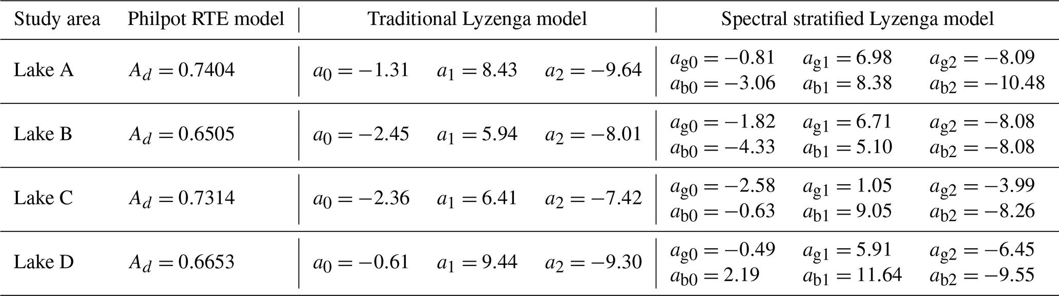
The study applies three bathymetry inversion models to the selected four SGLs for depth and volume estimation: the Philpot RTE model, the traditional Lyzenga model constrained by ICESat-2 points data, and the spectrally stratified, optimized Lyzenga model. The depth and volume results obtained from these three models are compared with ArcticDEM to demonstrate the effectiveness of the spectrally stratified algorithm applied in this study. The related model parameters used in this study is listed in Appendix A.

3.2.1 Radiative transfer equation model

The RTE model for bathymetry inversion was proposed by Philpot (1987). It is derived based on Beer-Lambert's law and has been widely applied in oceans and lakes. Its expression is shown in Eq. (2):

$$\begin{array}{}\text{(2)}& Z=g^{-\mathrm{1}}\left[\ln \left(A_d-R_{\mathrm{\infty }}\right)-\ln \left(R_{\mathit{\omega }}-R_{\mathrm{\infty }}\right)\right]\end{array}$$

where R_ω is the above-water surface reflectance; A_d is the bottom reflectance; g is a function of the diffuse attenuation coefficients for upward and downward radiance; R_∞ is the reflectance of infinitely deep water; and Z is the water depth.

In the Philpot RTE equation, the parameter determination follows previous studies. Specifically, A_d is calculated from averaging the reflectance values within a 30 m radius around each lake (Moussavi et al., 2016). However, ideal optically deep waters are typically absent within the GrIS region, making it difficult to obtain the reflectance values of spectral bands at infinite water depth. Therefore, following the approach of Melling et al. (2024), this study references the deep-water reflectance values of corresponding bands derived from multiple other Sentinel-2 scenes as substitutes. The values of g are typically adjusted to match the specific wavelengths observed by different satellite missions. The RTE equation is constructed using the reflectance of the green band due to its extended depth range and consistent depth-reflectance relationship up to approximately 10 m, following the approach of Lutz et al. (2024). Accordingly, the corresponding g value for the green band is 0.1413, as determined by Williamson et al. (2018) for Sentinel-2.

3.2.2 Traditional Lyzenga model

Both Lyzenga multi-band logarithmic linear model (Lyzenga, 1978, 1985) and Philpot RTE model exploit the exponential attenuation of light in water following Beer-Lambert's law, with Philpot RTE approach providing explicit physical parameterization of bottom reflectance and water column properties that were empirically combined in Lyzenga's earlier formulation. Unlike the purely theoretical RTE approach, which derives water depth only from optical imagery, this method introduces empirical constraints using a limited number of measured depth values to estimate model parameters. In this formulation, the bottom reflectance (A_d) and the diffuse attenuation coefficient function (g) are treated as constants, where a₀=ln (A_d-$R_{\mathrm{\infty }})/g$, $a_{\mathrm{1}}=-\mathrm{1}/g$, at this stage, the model equation is written as:

$$\begin{array}{}\text{(3)}& Z=a_{\mathrm{0}}+a_{\mathrm{1}}\left(R_{\mathit{\omega }}-R_{\mathrm{\infty }}\right)\end{array}$$

By integrating the spectral reflectance information from multiple bands, the following expression can be obtained:

$$\begin{array}{}\text{(4)}& Z=a_{\mathrm{0}}+\sum _{i=\mathrm{1}}^n{a}_i\ln \left[R_{\mathit{\omega }}\left({\mathit{\lambda }}_i\right)-R_{\mathrm{\infty }}\left({\mathit{\lambda }}_i\right)\right]\end{array}$$

This represents the commonly used Lyzenga model. In this study, ICESat-2 bathymetric points data together with green and blue band reflectance from Sentinel-2 are incorporated to constrain the empirical parameters of the Lyzenga model, and the parameter estimation is performed using the Levenberg–Marquardt (LM) algorithm.

3.2.3 Optimized Lyzenga model with spectral stratification

This study constructed a spectral stratified bathymetry inversion model based on the traditional Lyzenga model. By leveraging the varying penetration abilities of electromagnetic waves in water, the multispectral imagery was segmented into different layers, and zonal Lyzenga models were established for each layer in combination with ICESat-2 data. This study applied a spectral stratification method based on the Otsu algorithm, which automatically determines the optimal threshold without requiring user-defined parameters. The algorithm adaptively selects the threshold according to the statistical distribution of pixel intensities in the image histogram by maximizing the between-class variance and minimizing the within-class variance (Otsu, 1979). By utilizing the penetration characteristics and reflectance differences of water across different spectral bands, water in multispectral imagery was stratified into four layers: near-infrared, red, green, and blue bands. Specifically, the Otsu algorithm was first applied to determine the water extraction threshold in the near-infrared band. Subsequently, water in the near-infrared band was masked, and the same method was used to extract water in the red band. Next, both the near-infrared and red bands were masked to perform threshold segmentation for extracting water in the green band. Finally, by masking the extracted near-infrared, red, and green bands, water in the blue band was obtained, thereby achieving spectral stratification of the multispectral imagery (Fig. 4).

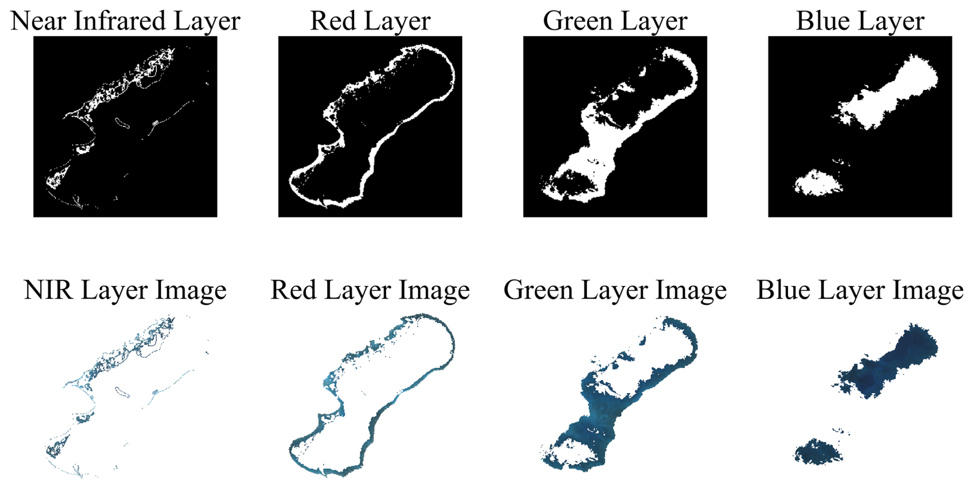
Figure 4 Binarized segmentation and spectral stratification of Lake A.The first row shows the mask images, and the second row shows the lake water bodies extracted using the masks.

Owing to the relatively small lake surface area of the near-infrared layer, the red layer, and the insufficiency of ICESat-2 bathymetry training photons in this study, the near-infrared layer, the red layer, and the green layer were combined for processing and collectively referred to as the green layer. In other words, the SGLs were divided into green and blue layers for bathymetry inversion, the expression was:

$$\begin{array}{}\text{(5)}& {\displaystyle }Z=a_{\mathrm{g}\mathrm{0}}+\sum _{i=\mathrm{1}}^N{a}_{\mathrm{gi}}\ln \left[R_{\mathit{\omega }}\left({\mathit{\lambda }}_i\right)-R_{\mathrm{\infty }}\left({\mathit{\lambda }}_i\right)\right]\text{(6)}& {\displaystyle }Z=a_{\mathrm{b}\mathrm{0}}+\sum _{i=\mathrm{1}}^N{a}_{\mathrm{bi}}\ln \left[R_{\mathit{\omega }}\left({\mathit{\lambda }}_i\right)-R_{\mathrm{\infty }}\left({\mathit{\lambda }}_i\right)\right]\end{array}$$

where Z is the predicted bathymetry result, a_g0 and a_gi are the corresponding parameters of the green layer, a_b0 and a_bi are the corresponding parameters of the blue layer.

3.3 Evaluation metrics

The bathymetric information derived from the above two bathymetry inversion models was validated and analysed using the ArcticDEM data as the reference. The coefficient of determination (R²), root mean square error (RMSE), and mean absolute error (MAE) between the two datasets were calculated to quantitatively validate the effectiveness of the proposed method (Hodson, 2022). The formulas for these metrics are as follows:

$$\begin{array}{}\text{(7)}& {\displaystyle }{R}^{\mathrm{2}}=\mathrm{1}-{\displaystyle \frac{\sum _{i=\mathrm{1}}^n{\left(h_i-\widehat{h}\right)}^{\mathrm{2}}}{\sum _{i=\mathrm{1}}^n{\left(h_i-\stackrel{\mathrm{‾}}{h}\right)}^{\mathrm{2}}}}\text{(8)}& {\displaystyle }\mathrm{RMSE}=\sqrt{{\displaystyle \frac{\sum _{i=\mathrm{1}}^n{\left(h_i-{\widehat{h}}_i\right)}^{\mathrm{2}}}{n}}}\text{(9)}& {\displaystyle }\mathrm{MAE}={\displaystyle \frac{\mathrm{1}}{n}}\sum \left|h_i-{\widehat{h}}_i\right|\end{array}$$

where ${\widehat{h}}_i$ is the predicted water depth, and h_i is the ArcticDEM-derived validation water depth and $\stackrel{\mathrm{‾}}{h}$ is the average value of the validation depth.

4 Result and analysis

Utilizing the datasets detailed in Sect. 2 and the bathymetry inversion methods outlined in Sect. 3, this section performs bathymetry inversion for Lakes A, B, C, and D. Additionally, the accuracy of the inversion results is validated and compared using ArcticDEM data. Section 4.1 and 4.2 presented both qualitative and quantitative evaluations of the bathymetry inversion results obtained from the Philpot RTE model, Lyzenga model, and the spectral stratified Lyzenga model to assess the feasibility and accuracy of the spectral stratified bathymetry inversion model.

4.1 Qualitative analysis

Figure 5 presents the bathymetry inversion results of the four supraglacial lakes obtained using the three proposed models. As shown in the figure, the water depths derived using the Philpot RTE model differ substantially from those obtained by the other two models, with generally higher depth estimates. In contrast, the water depth distributions derived from the Lyzenga model and the spectrally stratified Lyzenga model exhibit overall consistency, while certain local variations highlight the respective characteristics and performance of each model.

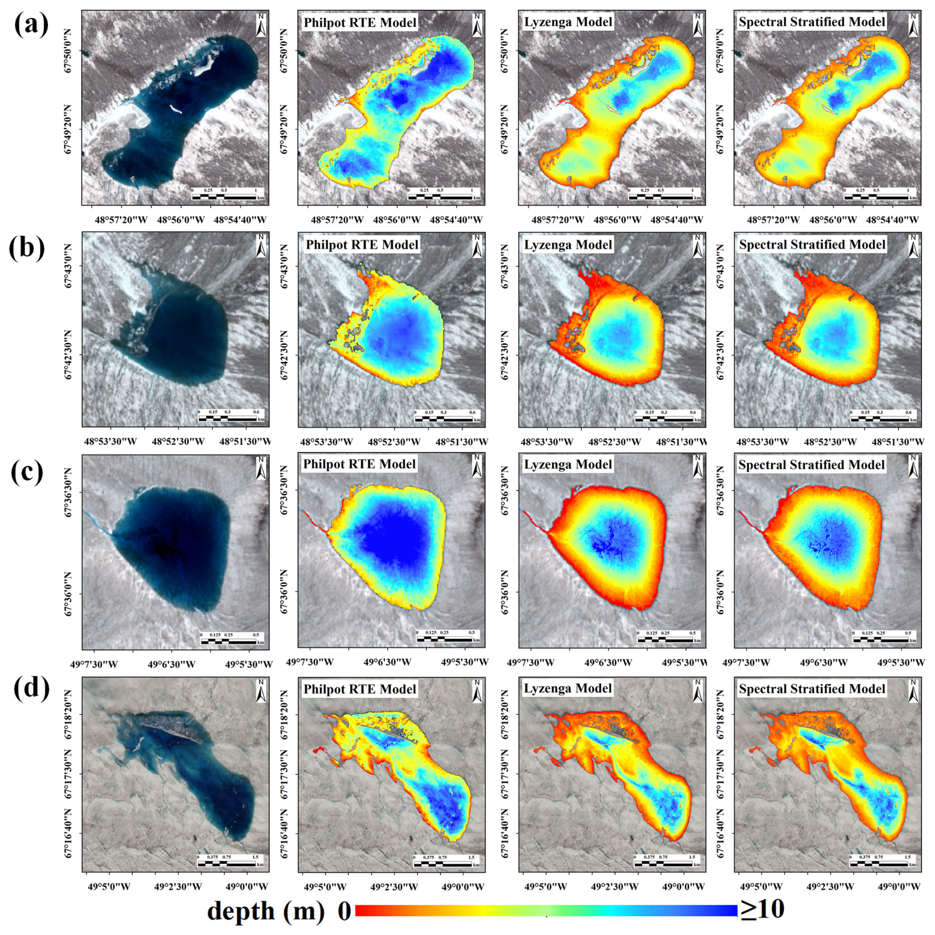
Figure 5 Lake bathymetry inversion results using the Philpot RTE model, the traditional Lyzenga model, and the spectral stratified Lyzenga model. (a) Lake A bathymetric inversion using the three models. (b) Lake B bathymetric inversion using the three models. (c) Lake C bathymetric inversion using the three model. (d) Lake D bathymetric inversion using the three models.

As shown in the Fig. 5, all the three bathymetric inversion models exhibit a similar pattern, with shallower depths around the lake margins and deeper areas toward the center, which aligns with intuitive expectations. However, the Philpot RTE model produces overall higher depth estimates compared with both the Lyzenga model and its spectral-stratified variant. The Lyzenga and spectral stratified Lyzenga models yield generally consistent results, although local discrepancies remain in certain areas. To further evaluate the performance differences among the models, residuals between the bathymetry derived from ArcticDEM and that obtained from each model were calculated for qualitative comparison. The spatial distribution of the residuals is illustrated in Fig. 6. In addition, since the ArcticDEM data only contain spatial information of the lake bottom, it lacks water surface elevation information when obtaining bathymetry benchmark data. Therefore, in this study, the edge position of the ArcticDEM lake was determined using ICESat-2 data, with this elevation serving as the water surface elevation.

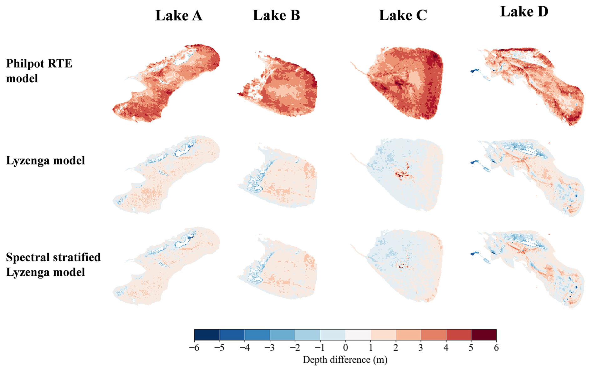
Figure 6 Differences between the water results derived from the three models and those obtained from ArcticDEM. Red areas indicate overestimation, while blue areas indicate underestimation.

The difference analysis shown in Fig. 6 further demonstrates that the Philpot RTE model tends to overestimate the overall water depth, while the Lyzenga model and the spectral stratified Lyzenga model exhibit varying degrees of overestimation and underestimation compared with ArcticDEM. Therefore, in addition to qualitative analysis, quantitative evaluation was also conducted to further assess and quantify the bathymetric results.

4.2 Quantitative analysis

To quantitatively and visually demonstrate the performance of the method, the validation results of the SDB using the traditional Lyzenga model and the spectrally stratified Lyzenga model are presented in Fig. 7.

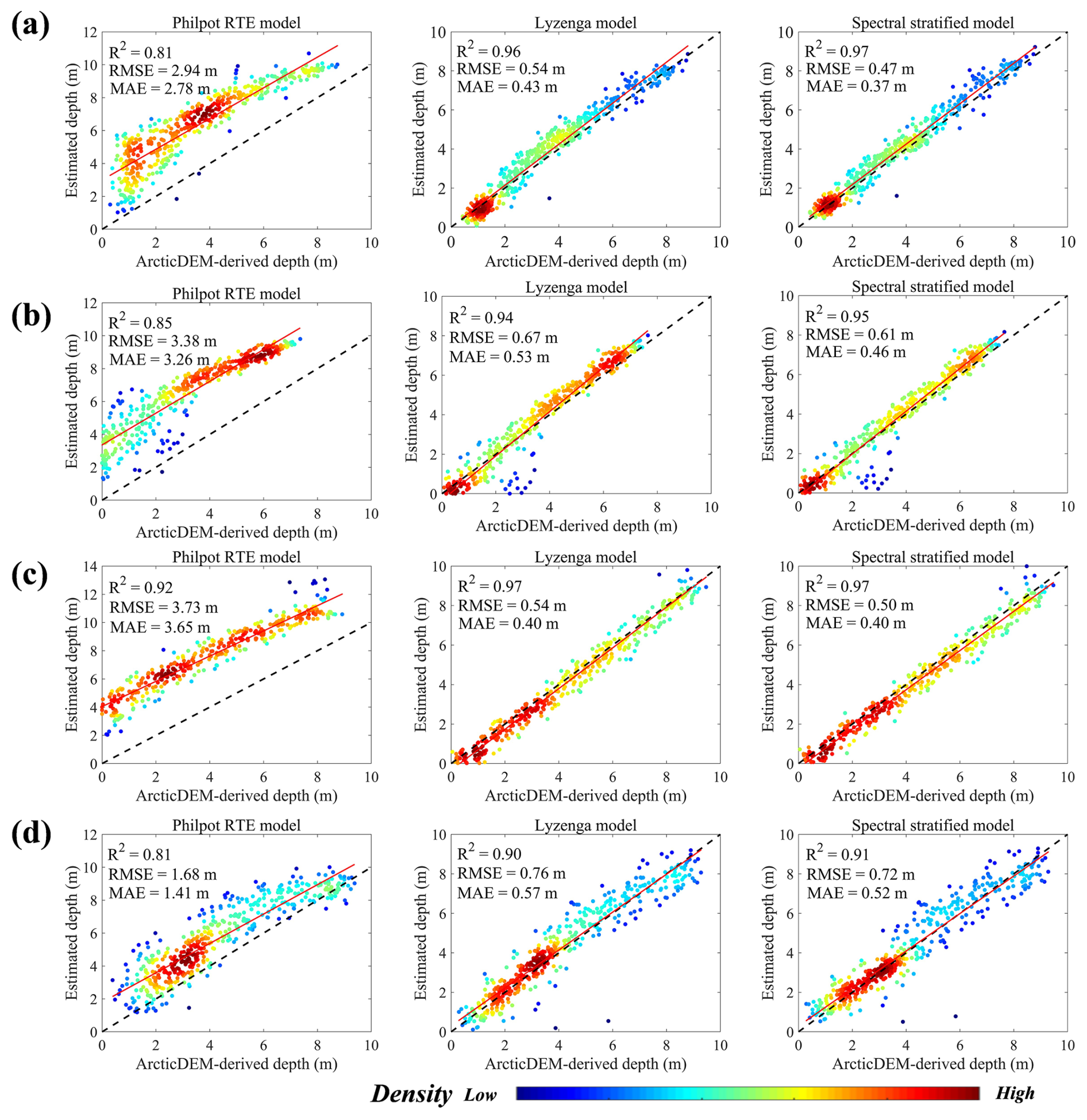
Figure 7 Comparison of SDB results using the Philpot RTE model, Lyzenga model, and spectral stratified Lyzenga model for the four lakes. (a) Lake A bathymetry validation. (b) Lake B bathymetry validation. (c) Lake C bathymetry validation. (d) Lake D bathymetry validation. The point represents the ArcticDEM validation points, the black dashed line indicates the 1:1 line, and the red solid line represents the data fitting line; the color bar indicates point density, defined as the number of validation points within a certain Euclidean neighborhood radius.

Table 2 Accuracy evaluation of the three models for the four lakes.

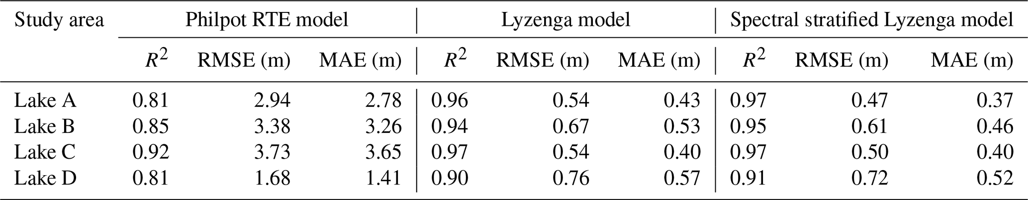
According to Fig. 7 and Table 2, the water depths derived from the Philpot RTE model show a clear overestimation compared with those from ArcticDEM, which is consistent with the qualitative differences revealed in Fig. 6. Although the RTE-derived depths exhibit relatively good correlation with ArcticDEM (with R² values exceeding 0.8), their RMSE and MAE remain relatively high. In contrast, both the Lyzenga model constrained by ICESat-2 data and its spectral stratified variant achieved higher accuracy. For all four lakes, the validation results showed R² values greater than or equal to 0.9, and RMSE and MAE within 10 % of the maximum lake depth. Specifically, for Lake A, the RMSE decreased to 0.47 m, representing reductions of 84.0 % and 13.0 % compared with the Philpot RTE model and the traditional Lyzenga model, respectively. The MAE decreased to 0.37 m, with reductions of 86.7 % and 14.0 %, respectively. For Lake B, the RMSE decreased to 0.61 m, reduced by 82.0 % and 9.0 %, while the MAE decreased to 0.46 m, reduced by 85.9 % and 13.2 %. For Lake C, the RMSE decreased to 0.50 m, reduced by 86.6 % and 7.4 %, and the MAE decreased to 0.40 m, reduced by 89.0 % compared with the Philpot RTE model. For Lake D, the RMSE decreased to 0.72 m, representing reductions of 57.1 % and 5.3 %, while the MAE decreased to 0.52 m, reduced by 63.1 % and 8.8 %, respectively. The validation results further demonstrate the effectiveness of the spectral stratification method in improving bathymetric inversion accuracy. In summary, the experimental results demonstrate that the spectral stratified method utilized in the study effectively improves the accuracy of bathymetry inversion for SGLs on the GrIS.

5 Discussion

5.1 Evaluation of the lake volume estimation

Based on the inverted bathymetry, the lake volume can be readily obtained by integrating the product of pixel area and water depth. In this study, the volumes derived from the Philpot RTE model, the Lyzenga model, and the spectral stratified Lyzenga model were calculated and compared with those obtained from ArcticDEM, as summarized in Table 3.

Table 3 Volume estimation based on the three models and comparison with ArcticDEM.

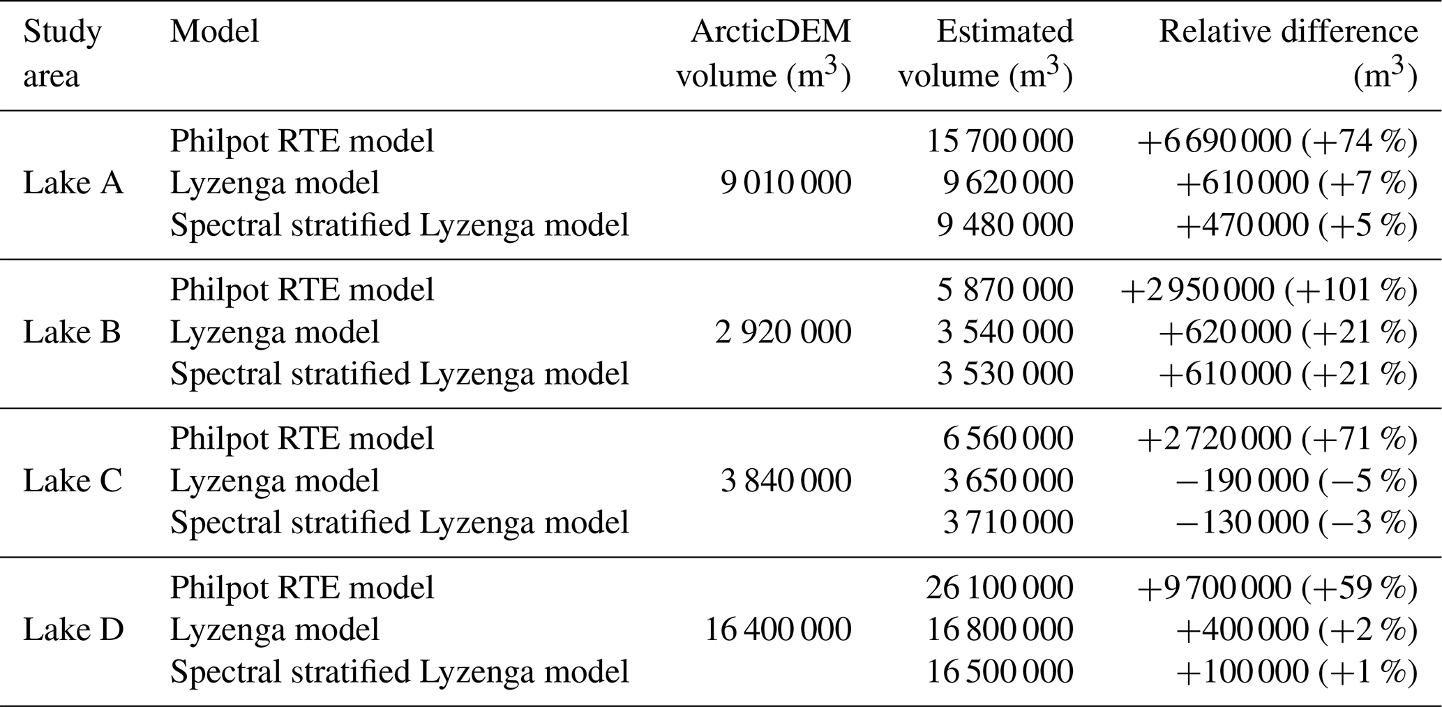
As shown in Table 3, the Philpot RTE model exhibited a consistent overestimation of lake volume across all four sites, ranging from 59 % to 101 %, which is considerably higher than those obtained from the Lyzenga and spectral stratified Lyzenga models. The latter two produced comparable results, with only minor differences observed for some lakes. Although the overall volume estimations derived from the spectral stratified Lyzenga model are close to those from the conventional Lyzenga model, the stratified approach offers a more physically interpretable framework by considering the spectral heterogeneity within the water body. In particular, this method allows each optical subset to be characterized by a separate empirical relationship, which may better reflect the inherent variations in water optical properties. While the improvement in total volume estimation is limited in this study, the model design provides a conceptually sound extension of the traditional Lyzenga model, and its potential advantages may become more evident in environments with stronger spatial or spectral variability. To facilitate the assessment of volume in Arctic SGLs, the volumes of lakes A, B, C, and D were derived through the 3D reconstruction method, as shown in Fig. 8. For a smoother visualization of the lake contours, Gaussian filtering was applied during the 3D reconstruction process.

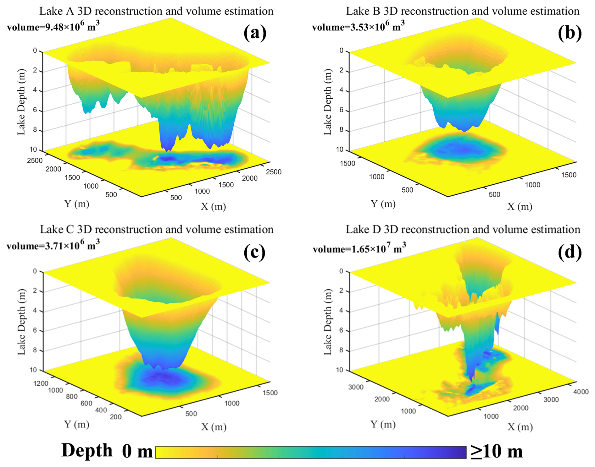
Figure 8 Volume estimation of the spectral stratified Lyzenga model bathymetry and 3D reconstruction of Lakes A, B, C, and D. (a) Lake A 3D reconstruction and volume estimation. (b) Lake B 3D reconstruction and volume estimation. (c) Lake C 3D reconstruction and volume estimation. (d) Lake D 3D reconstruction and volume estimation.

As shown in the Fig. 8, the volumes of Lake A, B, C, and D were 9.48×10⁶ m³, 3.53×10⁶ m³, 3.71×10⁶ m³, and 1.65×10⁷ m³. Compared to the sparse temporal coverage of ArcticDEM data, the method of calculating lake volume using bathymetry information obtained by the study approach is more effective and better meets the needs of accurate monitoring of lake volume. This new method provides a high-precision solution for the bathymetric inversion and volume estimation of SGLs in GrIS, offering data support for studies of glacier dynamics and lake hydrology. It also shows great potential for advanced applications, such as long-term monitoring of lake depth variations and hydrological characteristics (Lv et al., 2024), and for exploring their interactions with the surrounding ecological and environmental systems.

5.2 Challenges and limitations of the spectral stratification method

While the spectral stratification-based method enhances the accuracy of bathymetric inversion compared to traditional approaches, such as the Lyzenga model, several limitations need attention. First, the spatial distribution of ICESat-2 bathymetric samples is constrained by the orbital track layout, resulting in uneven sampling and limited spatial coverage. This restriction prevented full model training and made it necessary to combine the NIR, Red, and Green bands for model construction. Further improvement in accuracy could be achieved if additional stratification based on the Red band or other spectral combinations were introduced. Moreover, because SGLs on the GrIS are typically characterized by clear water, shallow depths, and stable substrates, the overall reflectance of the lake water shows little spatial variation. As a result, the influence of spectral penetration differences is limited, leading to only marginal accuracy improvements between the traditional Lyzenga model and the proposed spectral stratification model, as shown in Figs. 5 and 7. Second, the dynamic nature of the SGLs on the GrIS, which experience significant morphological changes over short periods, poses a challenge when combining ICESat-2 and Sentinel-2 data for bathymetric inversion. To achieve accurate results, the temporal synchronization of these data sets is critical, which places higher demands on data acquisition and availability. As a result, there is a limited pool of suitable ICESat-2 and Sentinel-2 data for conducting effective spectral bathymetric inversion in these lakes. Finally, the lake training strategy adopted in this study involves building individual models for each lake in combination with the spectral stratification approach. This design aims to improve the depth inversion accuracy for individual lakes and optimize existing traditional algorithms. Consequently, the model parameters proposed in this study cannot be directly transferred between different lakes. Nevertheless, the concept of spectral stratification introduced here is transferable and extensible. Whether applied to the Lyzenga model, the Stumpf model, or other machine learning approaches, this modeling framework based on spectral stratification can be readily incorporated. Addressing the current limitation of non-transferable model parameters by extending the framework to construct a large-scale, transferable, and high-precision bathymetric inversion model will be an important direction of our future work.

6 Conclusions

The study employed the spectral stratification method and the Otsu algorithm to determine reflectance thresholds across different bands, segmenting the lake's multispectral satellite imagery into distinct spectral layers. An optimized Lyzenga model based on spectral stratification was developed, and for comparison, the Philpot RTE model and the traditional Lyzenga model were also applied. For the four selected SGLs, the bathymetry inversion accuracy and volume-estimation errors derived by the three models were validated against the ArcticDEM data. The main conclusions are as follows:

1. Integrating the spectral stratification algorithm into the SDB method improves inversion accuracy. Compared with the Philpot RTE model, the RMSE and MAE were reduced by up to 86.6 % and 89.0 %, respectively; compared with the traditional Lyzenga model, the RMSE and MAE decreased by up to 13.0 % and 14.0 %, respectively, demonstrating the effectiveness of the spectral-stratification optimization strategy.

2. Compared with the Philpot RTE model, the spectral-stratified Lyzenga model applied in this study shows a noticeable improvement in lake volume estimation. However, when compared with the traditional Lyzenga model, the improvement is marginal and nearly negligible. This may be attributed to the approximately normal distribution of errors, which weakens the accuracy gains of the spectral stratified Lyzenga model during the additive process of volume estimation.

3. The spectral stratified SDB method requires high-quality data, with limited datasets suitable for SDB. For small, shallow SGLs, the optimization of inversion accuracy through spectral stratification is not significant, limiting improvements in inversion precision. Despite some limitations, the spectral stratified SDB method can effectively enhance the accuracy of SDB for SGLs, providing more timely and precise depth estimates. This approach offers valuable data support for studies of SGLs on the GrIS where in-situ depth measurements are challenging, and serves as a reference for research on environmental changes.

Appendix A

Table A1 Main core parameters used in the three bathymetry inversion models.