Physics-constrained generative machine learning-based high-resolution downscaling of Greenland's surface mass balance and surface temperature

Accurate, high-resolution projections of the Greenland ice sheet’s surface mass balance (SMB) and surface temperature are essential for understanding future sea-level rise, yet current approaches are either computationally demanding or limited to coarse spatial scales. Here, we introduce a novel physics-constrained generative modeling framework based on a consistency model (CM) to downscale low-resolution SMB and surface temperature fields by a factor of up to 32 (from 160 to 5 km grid spacing) in a few sampling steps. The CM is trained on monthly outputs of the regional climate model MARv3.12 and conditioned on ice-sheet topography and insolation. By enforcing a hard conservation constraint during inference, we ensure approximate preservation of SMB and temperature sums on the coarse spatial scale as well as robust generalization to extreme climate states without retraining. On the test set, our constrained CM achieves a continued ranked probability score of 5.37 $\mathrm{mm}\mathrm{w}.\mathrm{e}.$ per month for the SMB and 0.1 K for the surface temperature, outperforming interpolation-based downscaling. Together with spatial power-spectral analysis, we demonstrate that the CM faithfully reproduces variability across spatial scales. We further apply bias-corrected outputs of the NorESM2 Earth System Model and the Community Earth System Model CESM2-WACCM as inputs to our CM, to demonstrate the potential of our model to directly downscale ESM fields. Our approach delivers realistic, high-resolution climate forcing for ice-sheet simulations with fast inference and can be readily integrated into Earth-system and ice-sheet model workflows to improve projections of the future contribution to sea-level rise from Greenland and potentially other ice sheets and glaciers too.

1 Introduction

The Greenland ice sheet (GrIS) is the second largest ice sheet with an ice volume of 7.4 m sea level equivalent (Morlighem et al., 2017). Anthropogenic warming has driven a significant acceleration of Greenland mass loss over recent decades (Trusel et al., 2018). Currently, the mass loss of the GrIS is approximately evenly driven by dynamic discharge and a decrease in the surface mass balance (SMB), with ca. 60 % of GrIS ice loss due to the changes at the surface (van den Broeke et al., 2016; Choi et al., 2021). However, by the end of this century, the importance of surface processes is projected to increase as marine outlets retreat and dynamic processes will play a smaller role (Goelzer et al., 2020; Choi et al., 2021; Payne et al., 2021). That means that the SMB will be the determining factor of the overall mass balance of the GrIS. Modeling the GrIS surface mass balance demands fine resolution to capture the steep orographic gradients along the ice-sheet margin that govern precipitation patterns (Lucas-Picher et al., 2012). High-resolution simulations also resolve the narrow ablation zone and peripheral outlet glaciers, where most of the melt and runoff occur (Mottram et al., 2017). These high-resolution SMB fields then feed into ice-sheet model intercomparisons (e.g., ISMIP6), improving projections of dynamic thinning and sea-level contribution (Goelzer et al., 2020). Therefore, it is crucial to have realistic and high-resolution projections of the SMB in a changing climate.

Current methods to calculate the SMB have several disadvantages. They are either expensive to run, based on simple parameterisations or have low resolution. On short time scales, i.e., centennial scales, regional climate models such as MAR (Fettweis et al., 2013, 2017) or RACMO (van Dalum et al., 2024) are used to simulate the surface mass balance. These RCMs are specifically designed to simulate the polar regions. However, they are computationally expensive to run and are usually not accounting for a changing ice-sheet topography. On longer time scales, the SMB is usually simulated via simple parameterisation schemes such as the positive degree days method (PDD) (Aschwanden et al., 2019; Garbe et al., 2020; Beckmann and Winkelmann, 2023) or energy balance models (Zeitz et al., 2021; Bochow et al., 2023, 2024). Alternatively, the SMB can be directly derived from ESM runs as a sum of precipitation, runoff and evaporation in a first approximation (Seroussi et al., 2020; Nowicki et al., 2020). However, the ESM-derived SMB fields are limited to the, often coarse, resolution of the ESM and cannot resolve the steep gradients of the ice sheet, leading to biases in SMB estimates (Sellevold et al., 2019).

Given these computational constraints and resolution trade-offs across centennial and longer scales, computationally fast approaches are required to efficiently produce high-resolution SMB estimates. Previous approaches to downscaling the SMB of Greenland are often based on statistical downscaling (Noël et al., 2016; Tedesco et al., 2023). These approaches leverage the relationship between elevation, SMB and temperature, and have shown promising results in downscaling RCM results to higher resolutions. However, these statistical methods are inherently limited by their prescribed relationships between melt and elevation, which, for example, do not hold for the Antarctic ice sheet and can therefore not easily be extended to other regions (Tedesco et al., 2023). Additionally, these statistical methods cannot easily integrate complementary inputs that could improve the downscaling task (Tedesco et al., 2023). Therefore, novel machine-learning (ML) techniques, which can be trained to learn complex relationships, including topographic and climatological patterns, from high-resolution simulations and then run orders of magnitude faster are a promising approach. In contrast to previous statistical approaches, we aim to provide a framework in this work that is able to downscale SMB and T_s fields from other sources than RCMs, that is, deriving high-resolution fields directly from ESM output or from simpler physics-based models. Machine learning methods have gained tremendous attention in climate science in the last years, ranging from reconstruction of climate fields (Bochow et al., 2025), ML-based global circulation and weather models (Lam et al., 2023; Kochkov et al., 2024), downscaling (van der Meer et al., 2023; Hess et al., 2025) and weather forecasting (Bi et al., 2023; Price et al., 2025; Watt-Meyer et al., 2025). In the glaciological community, ML has, for example, been used to improve ice-flow simulations (Jouvet et al., 2022; Jouvet and Cordonnier, 2023), uncover flow laws of Antarctic ice shelves (Wang et al., 2025), improve upon traditional ice-shelf melt parameterisations (Rosier et al., 2023), forecast glacier-wide SMB (Bolibar et al., 2020; van der Meer et al., 2025; Steidl et al., 2025) or as emulators for subglacial hydrology models (Verjans and Robel, 2024).

Generative modeling approaches, and diffusion models in particular, have shown promising results in downscaling of ESM fields (Harris et al., 2022; Hess et al., 2023, 2025; Aich et al., 2024). The principle behind downscaling with generative diffusion models is based on so-called denoising, where a network is first trained to remove noise added to a high-resolution sample. Once trained, the network can then be applied for downscaling by iteratively generating realistic small-scale patterns from noise while following the large-scale patterns of the low-resolution ESM. However, most applications of generative downscaling so far are (i) limited to univariate fields (e.g. precipitation), (ii) struggle with training instabilities or mode collapse (Arjovsky and Bottou, 2017), (iii) require a large amount of sample steps to generate realistic fields (Bischoff and Deck, 2024) and/or (iv) lack physical mass conservation (Hess et al., 2025).

Here, we introduce a generative modeling-based methodology to derive high-resolution surface mass balance and temperature at the surface (T_s) fields for the Greenland ice sheet. The SMB and T_s are the most important, minimal surface forcing fields needed to drive an ice sheet model. We use a generative consistency model (CM) (Song et al., 2023; Hess et al., 2025) to demonstrate realistic and efficient downscaling of low-resolution SMB and temperature fields by at least a factor of 16 (Fig. 1, quadrupling the resolution gain of prior work, which was limited to a factor of 4 (Hess et al., 2025). In contrast to diffusion models that require dozens or even hundreds of time-steps, a CM directly learns a consistency function that maps a noised version of the target field back to its clean counterpart, allowing for fast generation of samples. By adding hard constraints during the sampling process, that is, local mass conservation of the SMB and conservation of T_s of the low-resolution field, we are able to generalize to more extreme climate conditions without the need for retraining. In theory, our model allows the simultaneous downscaling of arbitrarily many variables given high-quality training data. Compared to previous SMB downscaling approaches, our method does not explicitly prescribe any elevation-SMB relationship. It only requires coarse-resolution SMB and T_s fields, so the same trained model can be applied to inputs from different sources such as ESMs.

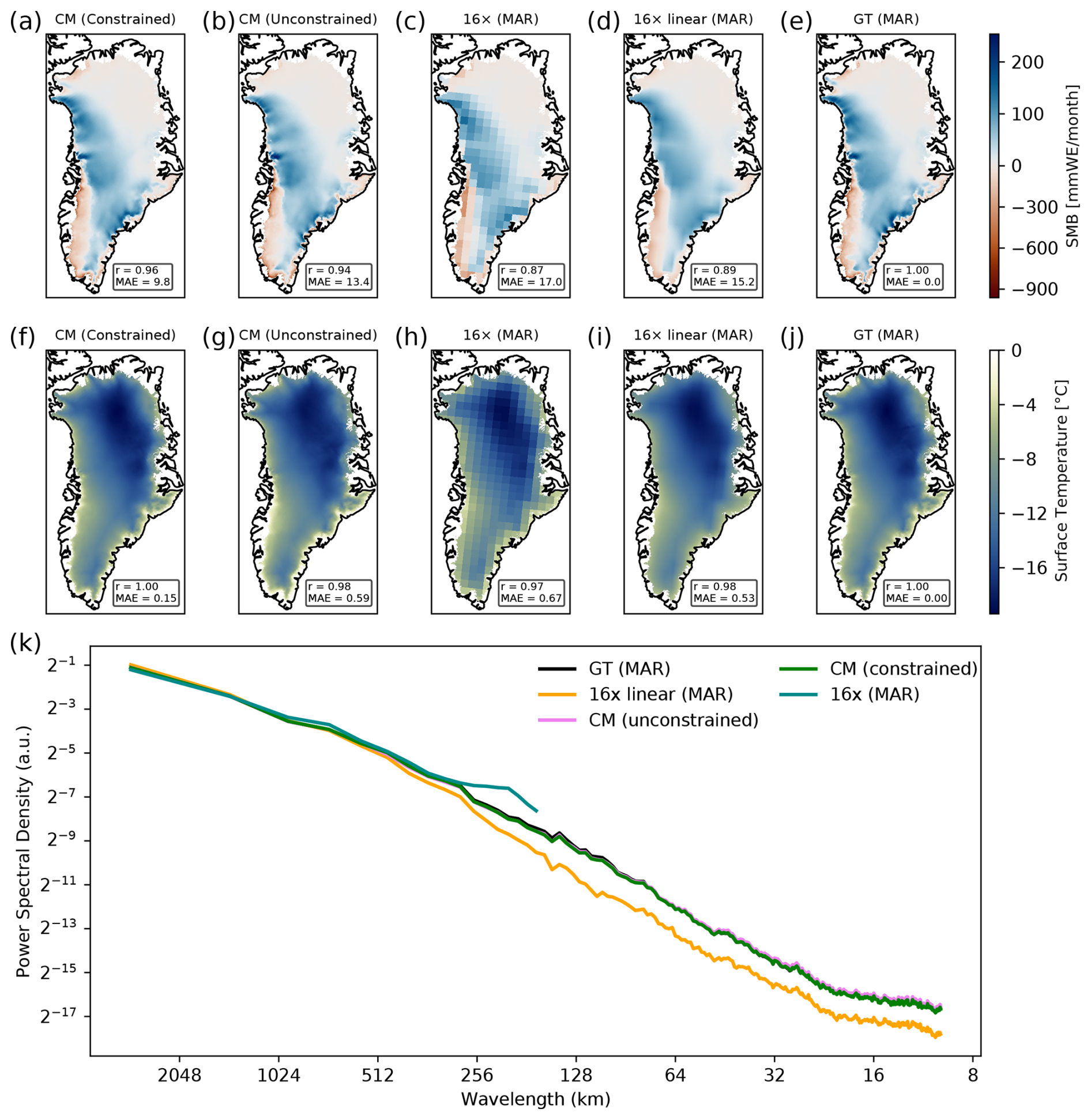
Figure 1 Qualitative comparison of downscaled SMB and T_s fields. (a) Downscaled SMB field of the test set with hard constraints during inference for a warm month with negative SMB at the margins (red) with a 5 km resolution. The mean absolute error (in $\mathrm{mm}\mathrm{w}.\mathrm{e}.$ per month) and Pearson correlation with the ground truth field are denoted. (b) Same as a but for the unconstrained CM. (c) We show the coarsened MAR field by a factor of 16 (80 km resolution), which is the input for the CM. The small scale variability is lost. (d) Same as (b) but linearly interpolated. (e) Ground truth MAR field with a 5 km resolution. (f–j) Same as (a)–(e) but for the surface temperature. (i) Radially averaged power spectral density of the whole test set for all depicted fields. The coarsened field has no small scale variability (blue). The linear interpolated field shows substantially lower small scale variability compared with the ground truth. The ground truth MAR field and CM fields almost show the same PSD.

We train our CM on high-resolution simulations of SMB and T_s from the regional climate model MARv3.12 (Fettweis et al., 2013, 2017). Once trained, the CM can be used to generate high-resolution SMB fields from ESM outputs using either directly the bias corrected SMB fields from the ESM or using a hybrid setup, combining the generative model with a positive degrees days (PDD) approach (Fig. 2). We are able to produce realistic SMB and T_s fields with a 5 km resolution openly available output from ESMs and MAR (Fig. 3). Ultimately, our methodology can be used for any climate field and potentially be directly integrated into ESMs.

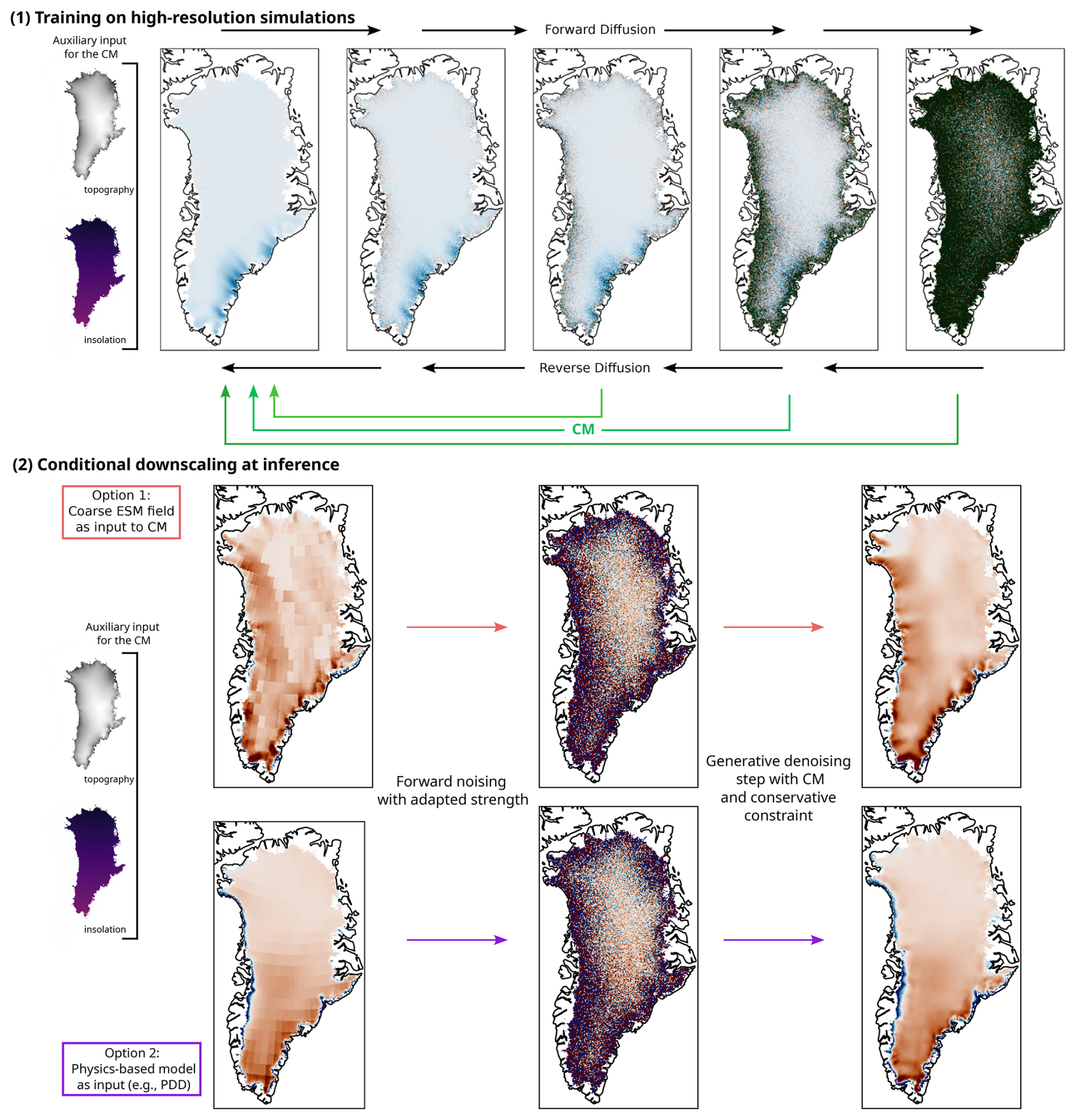
Figure 2 Schematic depiction of the consistency model (CM) workflow. We train the CM on the high-resolution RCM MARv3.12 with the topography and insolation as auxiliary inputs. During the inference, the low resolution input fields are noised with an adaptive noising strength and subsequently denoised by the trained CM with conservative constraints. The small-scale variability is recovered by the CM.

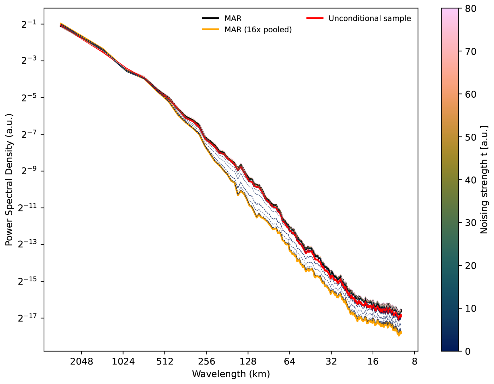
Figure 3 Normalized power spectral density (PSD) for different noise scales. The mean radially averaged normalized PSD for different noising scales is shown. We downscale the test set that was coarsened by a factor of 16 and linearly interpolated using the CM (unconstrained). Additionally, the PSD of an unconditional ensemble is shown (red). The coarsened field (orange) generally underestimates the small scale variability, i.e., the variability below 512 km. The higher the noising scale, the more the PSD of the downscaled fields resembles the PSD of the original field (black). Larger noise scales correspond to less pairing with the initial fields.

2 Methods and Data

2.1 Consistency model

We use a consistency model architecture (Song et al., 2023), recently introduced for downscaling (Hess et al., 2025) to derive high-resolution SMB and temperature fields. CMs are inspired by iterative diffusion models (Ho et al., 2020; Song et al., 2021), but offer several advantages. The idea behind CM is to learn a direct mapping from noisy inputs to clean data such that any point along the same noise trajectory (for the same underlying data) maps to the same clean state (Song et al., 2023). In contrast to previously introduced diffusion models, which need many evaluation steps (usually in the range of 10–2000) to generate realistic samples, CM can therefore generate realistic samples in only one step. Consistency models learn a consistency function $f\left(x\right(t),t,y)=x\left(t_{\text{min}}\right)$, which is self consistent:

$$\begin{array}{}\text{(1)}& f\left(\mathbf{x}\right(t),t,\mathbf{y})=f\left(\mathbf{x}\right(t^{\prime }),t^{\prime },\mathbf{y})\forall t,t^{\prime }\in [t_{min},t_{max}],\end{array}$$

with the time-independent conditioning fields y, the input fields x(t), i.e., the T_s and SMB and the time t. That is, the model’s output is invariant to the noise level. Following Song et al. (2023) and Hess et al. (2025), we set t_min=0.002 and t_max=80. We impose the boundary condition $f\left(x\right(t_{\text{min}}),t_{\text{min}})=x\left(t_{\text{min}}\right)$ for t=t_min. This is parameterised in the model via skip connections

$$\begin{array}{}\text{(2)}& f(\mathbf{x},t,\mathbf{y};\mathit{\theta })=c_{\text{skip}}\left(t\right)\mathbf{x}+c_{\text{out}}\left(t\right)F(\mathbf{x},t,\mathbf{y};\mathit{\theta }),\end{array}$$

where F(⋅) is a U-Net (Ronneberger et al., 2015) with parameter θ. A U-Net is a convolutional neural network architecture with skip connections between the encoder and decoder part (Ronneberger et al., 2015; Song et al., 2021).

The parameters c_skip and c_out are defined as

$$\begin{array}{}\text{(3)}& c_{\text{skip}}={\displaystyle \frac{{\mathit{\sigma }}_{\text{data}}^{\mathrm{2}}}{\left((t-t_{min}{)}^{\mathrm{2}}+{\mathit{\sigma }}_{\text{data}}^{\mathrm{2}}\right)}},c_{\text{out}}\left(t\right)={\displaystyle \frac{{\mathit{\sigma }}_{\text{data}}t}{\sqrt{t^{\mathrm{2}}+{\mathit{\sigma }}_{{\text{data}}^{\mathrm{2}}}}}}.\end{array}$$

The consistency training objective is given by (Song et al., 2023)

$$\begin{array}{}\text{(4)}& \begin{array}{rl}& \mathcal{L}(\mathit{\theta },\stackrel{\mathrm{‾}}{\mathit{\theta }})=\\ & {\mathbb{E}}_{\mathbf{x},n,t_n}\left[d\left(f(\mathbf{x}+t_{n+\mathrm{1}}\mathbf{z},t_{n+\mathrm{1}},\mathbf{y};\mathit{\theta }),f\left(\mathbf{x}+t_n\mathbf{z},t_n,\mathbf{y};\stackrel{\mathrm{‾}}{\mathit{\theta }}\right)\right)\right].\end{array}\end{array}$$

The distance measure $d(\cdot ,\cdot )$ is given by $d(\mathbf{x},\mathbf{y})=\text{LPIPS}(\mathbf{x},\mathbf{y})+\left|\right|\mathbf{x}-\mathbf{y}|{|}_{\mathrm{1}}$ (Song et al., 2023; Hess et al., 2025), where LPIPS is the Learned Perceptual Image Patch Similarity (Zhang et al., 2018).

The training objective is minimized by stochastic gradient descent (Adam optimizer) on the model parameters θ, while $\stackrel{\mathrm{‾}}{\mathit{\theta }}$ denotes an exponential moving average (EMA) over the model parameters:

$$\begin{array}{}\text{(5)}& \stackrel{\mathrm{‾}}{\mathit{\theta }}=\text{stopgrad}\left[w\right(k)\stackrel{\mathrm{‾}}{\mathit{\theta }}+(\mathrm{1}-w\left(k\right)\mathit{\theta }\left)\right].\end{array}$$

The decay schedule w(k) is given by

$$\begin{array}{}\text{(6)}& w\left(k\right)=\exp \left({\displaystyle \frac{s_{\mathrm{0}}\log \left(w_{\mathrm{0}}\right)}{N\left(k\right)}}\right),\end{array}$$

with w₀=0.9. The EMA has been found to greatly stabilize training and improve final performance of the CM (Song et al., 2023).

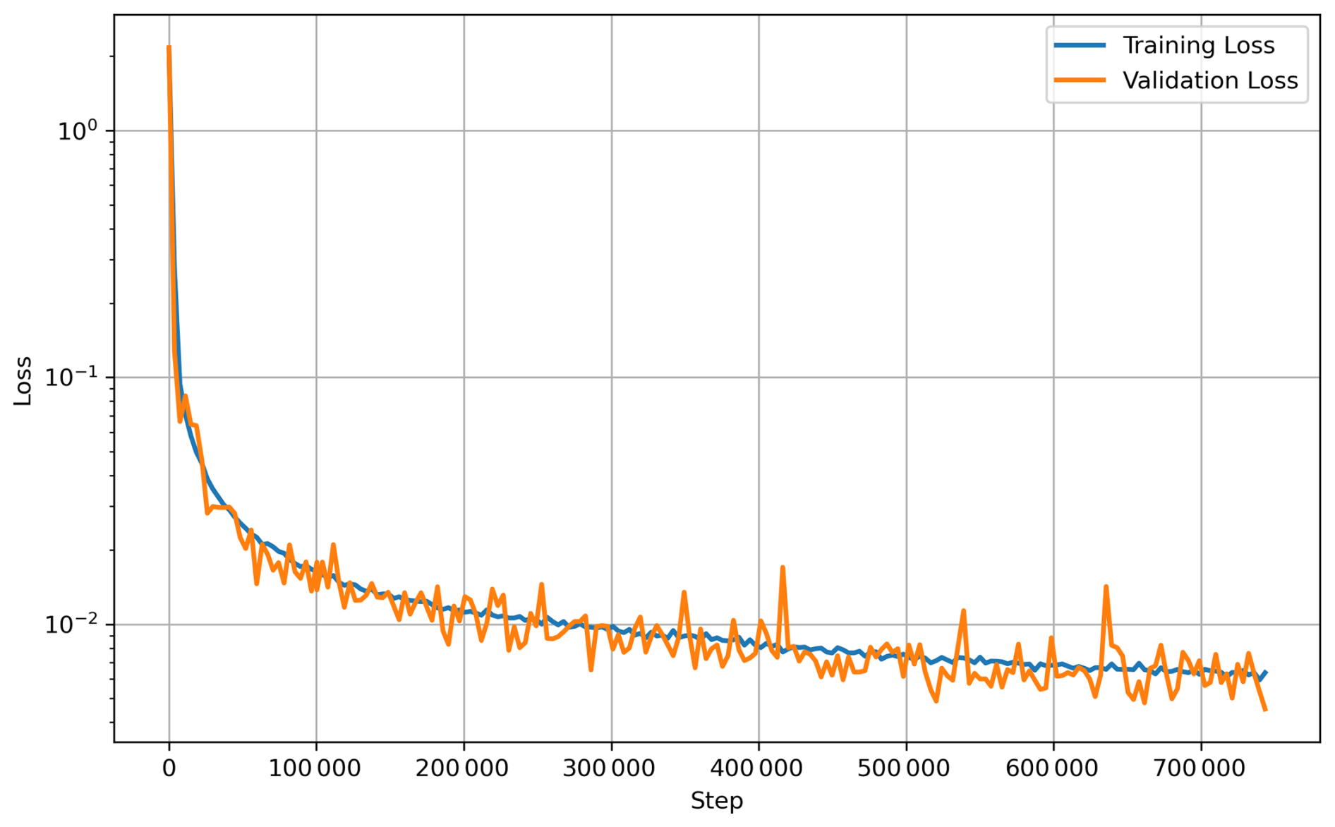
While, CMs can be distilled from diffusion models, we train the model from scratch. We use the same U-Net backbone as in Hess et al. (2025). We train for 200 epochs with a batch size of 4 with 21 432 samples in the training set in total. We choose this relatively small batch size due to GPU memory constraints. Training on a single NVIDIA H100 Tensor Core GPU takes approximately 5 d.

While, CMs can generate samples in only one step, we use multi-step sampling (max. 10 steps) to enhance sample quality and avoid artifacts (Song et al., 2023). Starting from an initial noisy input, we progressively add scaled Gaussian noise at discrete time steps and denoise the field using the CM. One evaluation, i.e. downscaling one monthly field, for t=5 with hard constraining takes ca. 1.6 s on a NVIDIA H100 Tensor Core GPU.

Downscaling 85 years of monthly SMB and surface temperature fields with the constrained CM takes approximately 30 min on a single NVIDIA H100 Tensor Core GPU, where transformation and saving of the data takes up the most time. While the training of the CM takes several days on a single high-end GPU, the downscaling itself is therefore computationally very efficient. Running the CM is straightforward and just requires the low-resolution SMB and T_s input fields on the 5 km ISMIP6 grid.

2.2 Bias correction

We use Quantile Data Mapping (QDM) for bias correcting the ESM fields when used as input for the PDD or CM using the Python library xclim (Bourgault et al., 2023), which follows the algorithm introduced by Cannon et al. (2015). The idea of QDM is to correct systematic biases in modeled time series compared to a reference period of observed data or ground truth (here the RCM MAR) while conserving model-projected relative changes in quantiles (Cannon et al., 2015). It is applied for each spatial grid cell and variable individually. The QDM algorithm uses two steps. First, the future model output is detrended by quantile and bias corrected to the reference data by quantile mapping. Second, the absolute or relative change in quantiles is superimposed on the bias-corrected model output. The time-dependent cumulative density function (CDF) τ_m,p(t)=F_t(x_m,p(t)) of the modeled projected time series x_m,p over a time window is calculated (e.g., the future period). The relative change in quantiles between the modeled reference period ref and a future time t is given by

$$\begin{array}{}\text{(7)}& {\mathrm{\Delta }}_{\mathrm{m}}\left(t\right)={\displaystyle \frac{F_t^{-\mathrm{1}}\left({\mathit{\tau }}_{\text{m,p}}\right(t\left)\right)}{F^{(-\mathrm{1})}\left({\mathit{\tau }}_{\text{m,ref}}\right(t\left)\right)}}={\displaystyle \frac{x_{\text{m,p}}\left(t\right)}{F^{(-\mathrm{1})}\left({\mathit{\tau }}_{\text{m,ref}}\right(t\left)\right)}}\end{array}$$

with the inverse CDF F⁻¹. The modeled τ_m,p(t) quantile is then bias corrected by applying the inverse CDF derived from the observed values over the reference period

$$\begin{array}{}\text{(8)}& {\widehat{x}}_{\text{o:m,ref:p}}\left(t\right)=F_{\text{o,ref}}^{(-\mathrm{1})}\left({\mathit{\tau }}_{\text{m,p}}\right(t\left)\right).\end{array}$$

Finally, the bias-corrected modeled projected time series at time ${\widehat{x}}_{\text{m,p}}\left(t\right)$ is given by

$$\begin{array}{}\text{(9)}& {\widehat{x}}_{\text{m,p}}={\widehat{x}}_{\text{o:m,ref:p}}\left(t\right)+{\mathrm{\Delta }}_{\mathrm{m}}\left(t\right).\end{array}$$

We use 100 quantiles and do a monthly-based bias correction.

2.3 Conservation constraints

To allow the CM to downscale fields that are far out-of-sample, we implement the option to enforce a hard conservation constraint during the inference (Harder et al., 2023). This does not require a retraining of the CM.

The initial conditions are pooled using adaptive pooling with a factor that should correspond to the resolution ratio between the low and high resolution fields. This gives a field with so-called superblocks, i.e., pooled pixels. The first denoising step is not changed and gives a first guess of the downscaled field. After the first denoising step, we add the residual between each superblock and the corresponding high-resolution pixels. That is, to each intermediate output pixel during the multistep sampling ${\stackrel{\mathrm{̃}}{y}}_i$ the residual between the superblock x and the mean of the corresponding pixels $\frac{\mathrm{1}}{n}{\sum }_{i=\mathrm{1}}^n{\stackrel{\mathrm{̃}}{y}}_i$ is added:

$$\begin{array}{}\text{(10)}& y_j={\stackrel{\mathrm{̃}}{y}}_j+x-{\displaystyle \frac{\mathrm{1}}{n}}\sum _{i=\mathrm{1}}^n{\stackrel{\mathrm{̃}}{y}}_i.\end{array}$$

The residuals are corrected to account for the number of land pixels in each superblocks. That is, the residuals are only distributed onto the valid GrIS pixels and not into the ocean. In the last denoising step, we do not enforce this constraint. To avoid artifacts in the downscaled field due to the pooling step, we use the area interpolation and Gaussian filter on the residual field before adding the residual field in each step.

To avoid cases where all residuals of a superblock are distributed to only a few pixels of the GrIS, which would lead to unrealistic SMB values at the GrIS margins, we implement a simple greedy region-growing algorithm. Each superblock cell that has less than a chosen number of corresponding land pixels in the high-resolution field (we choose 16² pixels) annexes its largest neighboring blocks until it exceeds the chosen threshold. This continues until all superblocks are assigned a region with at least 16² pixels. We find that 16²–32² pixels is a reasonable choice ensuring realistic fields and avoiding artifacts in the downscaled fields.

Since the conservation of the SMB should happen in physical units, we transform the correction field and intermediate fields back to physical units before we apply the constraint. Subsequently, we transform the fields back to the transformed units before running the next step of the CM.

2.4 PDD Model

We use a simple positive degree day (PDD) model based on the PyPDD implementation (Seguinot, 2019). The PDD is a semi-physical method that takes the precipitation and the near-surface air temperature as input and estimates the surface mass balance. Here, we use the temperature at 2 m height (tas in CMIP6) and the total precipitation (pr) as input variables. Specifically, the PDD are calculated according to (Seguinot, 2013; Calov and Greve, 2005)

$$\begin{array}{}\text{(11)}& \begin{array}{rl}& \text{PDD}=\\ & \underset{\mathrm{0}}{\overset{A}{\int }}\left[{\displaystyle \frac{\mathit{\sigma }}{\sqrt{\mathrm{2}\mathit{\pi }}}}\exp \left(-{\displaystyle \frac{T_{\text{ac}}(t{)}^{\mathrm{2}}}{\mathrm{2}{\mathit{\sigma }}^{\mathrm{2}}}}\right)+{\displaystyle \frac{T_{\text{ac}}\left(t\right)}{\mathrm{2}}}\text{erfc}\left(-{\displaystyle \frac{T_{\text{ac}}\left(t\right)}{\sqrt{\mathrm{2}}\mathit{\sigma }}}\right)\right]\mathrm{d}t,\end{array}\end{array}$$

with the time interval A, the time-dependent seasonal near-surface temperature T_ac(t), the standard deviation of the temperature σ=5 K and the error function erfc. Following the standard conventions, we assume that all precipitation contributes to snow accumulation whenever air temperature T≤0 °C, and that the snow-fraction (hence accumulation) declines linearly to zero as T rises from 0 to 2 °C. Melt is then calculated via positive degree-day factors of 3 $\mathrm{mm}\mathrm{°}{\mathrm{C}}^{-\mathrm{1}}{\mathrm{d}}^{-\mathrm{1}}$ for snow and 8 $\mathrm{mm}\mathrm{°}{\mathrm{C}}^{-\mathrm{1}}{\mathrm{d}}^{-\mathrm{1}}$ for ice. For more details we refer to Seguinot (2013).

2.5 Training

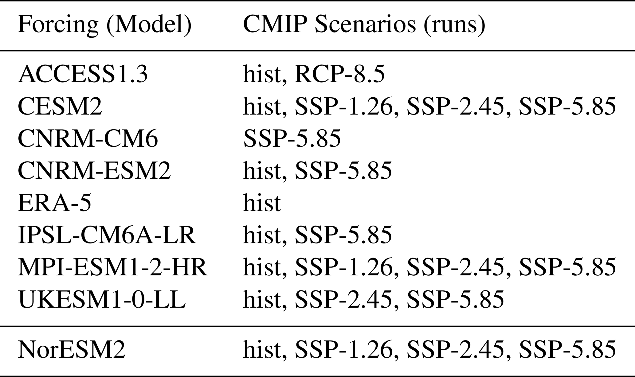
We use monthly output from the regional climate model Modèle Atmosphérique Régional (MAR) version 3.12 forced by different Earth system models (Table 1) over the time period 1950–2100 (Fettweis et al., 2013, 2017). In total we use 23 different model runs, totaling to 21 432 monthly fields. We hold out 4 independent runs from MAR forced by the ESM NorESM2 (Seland et al., 2020) for additional testing. We regrid the MAR fields to 5 km resolution, corresponding to the IMSIP6 grid (Goelzer et al., 2020). Additionally, we mask the fields with the current ice sheet mask given by MAR, that is, we set the SMB to 0 outside of the current ice sheet geometry.

Table 1 Selected MARv3.12 runs for the training forced by CMIP5 and CMIP6 models. All models used for training and the respective scenario are denoted. The MAR runs forced by NorESM are held out for validation.

We condition our CM on the ice sheet height and the spatially-varying monthly mean insolation as additional input besides the SMB. The monthly mean insolation is calculated by averaging the mean daily insolation over each month following Hartmann (1994). This ensures that generated unconditional samples, i.e., samples without initial conditions, adhere to the topography of the GrIS. The insolation allows the CM to learn the seasonal melt cycle to some extent and generate unconditional samples that adhere to it. The input fields are simply concatenated before being fed to the U-Net.

Additionally, we find that oversampling years after 2080 during training leads to better generalization to extreme climate states during testing. This is because the MAR simulations show much stronger melt (more negative SMB) rates after 2080 compared to the historical period. Therefore, we oversample years after 2080 by a factor of 10 during training.

2.6 Noising scale

During inference, noise is added to the climate fields to remove spatial patterns, which are subsequently filled in by the trained CM. Adding Gaussian noise with a chosen variance removes spatial patterns up to a spatial scale associated with the added noise (Hess et al., 2025). The more noise is added, the more spatial structure in the input field is removed. The goal is to find an optimal noising scale that recovers small-scale variability while maintaining a reasonable correspondence to the initial field. To determine the optimal noising scale, which reasonably recovers the small-scale variability while also providing the smallest errors, we generate an ensemble of 50 realisations and evaluate the power spectral density (PSD) and the continuous ranked probability score (CRPS) for different noising scales. While the PSD is a measure of the variability on varying spatial scales, the CRPS is a metric that compares the ground truth to an ensemble of predictions. It can be seen as a probabilistic generalization of the mean absolute error.

2.7 Validation and projections

We evaluate our model on two ESMs, the Norwegian Earth system model (NorESM2) (Seland et al., 2020) under the SSP-5.85 forcing until the year 2100 and the Community Earth System Model version 2 with the Whole Atmosphere Community Climate Model (CESM2-WACCM) under the extended high-emission SSP-5.85 scenario from the year 2015 to the year 2300 (Gettelman et al., 2019; Danabasoglu et al., 2020). Like most ESMs, the NorESM2 does not directly provide a SMB field. However, the SMB can be approximated as the sum of precipitation, evaporation and runoff (Seroussi et al., 2020; Nowicki et al., 2020). Naturally, the CM is then able to directly downscale from this first approximation of the SMB. In constrast to NorESM2, the CESM2-WACCM runs directly provide monthly SMB fields (variable name acabf) in addition to the near-surface temperature (ts) fields. For both models, we bias correct the surface temperature as well as the SMB fields using Quantile Data Mapping (QDM) with the MAR fields driven by the reanalysis ERA5, using the historical period 1950–2015 as the reference period. For the NorESM2 run, there is a corresponding MAR run. However, it should be noted that the fields are not paired in the strict sense since MAR is driven by other variables and hence the spatial patterns do not necessarily match. For CESM2-WACCM we do not have a corresponding MAR run.

3 Results

We provide a generative machine-learning based method, that is able to downscale SMB and temperature fields T_s simultaneously. We include the ice sheet height and the monthly average of the insolation as additional conditioning input. Additionally, we implement a hard conservation constraint during inference to conserve the SMB and temperature on a regional level during the downscaling (cf. Methods). If not explicitly stated differently, we always show the hard-constrained CM version. In the following, we concentrate on the SMB downscaling task, since downscaling the temperature is generally easier due to the relative smoothness of the temperature fields. The model workflow is depicted in Fig. A1. We use monthly output from the RCM MARv3.12 forced by different ESMs over the time period 1950–2100 (Table 1), in total 23 model runs, i.e., 21 432 monthly fields (cf. Methods).

Here, we evaluate how our model performs on two different downscaling tasks. First, we show the downscaling results of the CM using artificially coarsened MAR test set data. This has the advantage that we have paired low- and high-resolution fields for evaluations. Secondly, we show how the CM can be used to derive high-resolution SMB and T_s fields directly from unpaired low-resolution ESM output.

3.1 Downscaling low-resolution MAR

The held-out test set consists of 16 random years between the time period 1950 and 2100. In total, 2448 months have been held out from the train and validation set.

To test the ability of the CM to downscale from low to high resolution, we first coarsen the MAR fields by a factor of 16, that is, 16 times lower resolution than the high-resolution fields (80 km×80 km). This corresponds to a typical spatial resolution as provided by state-of-the-art ESMs. We downscale these pooled fields with our CM to recover the small-scale variability.

Both the downscaled SMB and T_s fields are visually similar to the ground truth, while the linearly interpolated fields show a reduced small-scale variability (Figs. 1 and 3). To quantitatively evaluate how well the CM is able to reconstruct the small-scale variability of the SMB fields, we calculate the radially averaged power spectral density (PSD) following Ravuri et al. (2021); Hess et al. (2023, 2025). The coarse field shows no small-scale variability (blue), while the linearly interpolated field shows a substantial underestimation of the small-scale variability (orange). In contrast, the downscaled fields using the CM show a highly accurate representation of small-scale variability compared to the ground truth. In particular, the PSD of the hard-constrained field (CM HC) is indistinguishable from the ground truth.

The hard-constrained fields show the best performance compared to the ground truth MAR over the whole test set in terms of the error metrics (MAE=9.9 $\mathrm{mm}\mathrm{w}.\mathrm{e}.$ per month and r=0.98). The unconstrained downscaled field shows worse performance (MAE=15.5 $\mathrm{mm}\mathrm{w}.\mathrm{e}.$ per month and r=0.96). For comparison, the linearly interpolated field performs slightly worse than the unconstrained CM fields (MAE=17.6 $\mathrm{mm}\mathrm{w}.\mathrm{e}.$ per month, r=0.93) Similarly, the hard-constrained downscaled T_s field shows the lowest errors and highest correlation relative to the ground truth (MAE=0.19 K, r=1.00). Again, the unconstrained downscaled field shows a worse performance in terms of the error metrics (MAE=0.83 K, r=1.00). For comparison, the linearly interpolated field of the temperature shows better metrics than the unconstrained fields (MAE=0.69 K, r=1.0; Fig. 1j).

Additionally, we coarsen the MAR fields by a factor 32 (160 km resolution) and show that the CM, in principle, still can downscale the fields (Fig. B4). While the performance of the CM is still better than simply linearly interpolating, it is worse than for the downscaled field from the coarsened field by factor 16. The integrated monthly SMB is still mostly conserved with a residual of less than 25 Gt for almost all months (Fig. B4b). However, due to the very coarse resolution of the input field, some information is lost during the coarsening process. The error is largest at the margins, especially the southeastern margin (Fig. B4c and d). It should be noted that due to the coarse resolution and the overall conservation of the per-cell SMB, the pixel edges are slightly visible in the MAE and the output fields. This is, for example, visible in southwestern Greenland with negative SMB in Fig. B4e, where the relatively sharp edge from the coarse field (Fig. B4f) propagates into the downscaled field. This is per construction due to the hard-constraining but could be improved by using the linearly interpolated field as input with the tradeoff of losing information due to the interpolation process. However, the small spatial scales are still substantially better resolved than in the linearly interpolated field and the error is generally lower (Fig. B4g).

3.1.1 Generalizability to extreme climates

Our approach also permits downscaling of fields that are at the far end of the SMB distribution, that is, for high-emission scenarios at the end of this century with extremely negative SMB for most of Greenland. While the unconstrained model underestimates the melt or overestimates the SMB for most of Greenland to some extent (Fig. B1b), the constrained version is able to realistically downscale the SMB field (Fig. B1a). The MAE for one realization of this specific month is 38 % lower for the constrained CM (MAE=57.0 $\mathrm{mm}\mathrm{w}.\mathrm{e}.$ per month) than for a simple linear interpolation (MAE=90.7 $\mathrm{mm}\mathrm{w}.\mathrm{e}.$ per month). Similarly, the correlation is higher for the constrained CM. The MAE of the unconstrained model (MAE=78.1 $\mathrm{mm}\mathrm{w}.\mathrm{e}.$ per month and r=0.97) is higher than for the constrained CM but still lower than for the coarsened field (MAE=104.9 $\mathrm{mm}\mathrm{w}.\mathrm{e}.$ per month and r=0.93).

For the temperature fields, the CM constrained field shows the best metrics (Fig. B1i). The MAE of the constrained CM is ca. 20 % lower (MAE=0.14 K) than for the linearly interpolated field (MAE=0.18 K). The unconstrained version shows a worse performance than the linearly interpolated field (MAE=0.48 K) (Fig. B1g). By hard-constraining the CM, the downscaled fields approximately conserve the SMB even for very negative SMB (Fig. 4). The maximum absolute error in the monthly integrated SMB of the downscaled field over the whole ice sheet compared to the ground truth is 6.8 Gt. In contrast, linearly interpolating the coarsened fields leads to a clear overestimation of the SMB for very negative SMB fields (Fig. 4b). For comparison, the maximum absolute error of the integrated SMB of the linearly interpolated field is 86.6 Gt. For small noising scales (t<1) the CM reproduces the hard boundaries of the pooled fields, which can be avoided by linearly interpolating the fields before feeding into the CM. However, since linear interpolation is not a conserving operation, this leads to a minor loss of information, which ultimately leads to worse quality of the downscaled fields compared to directly downscaling the pooled fields.

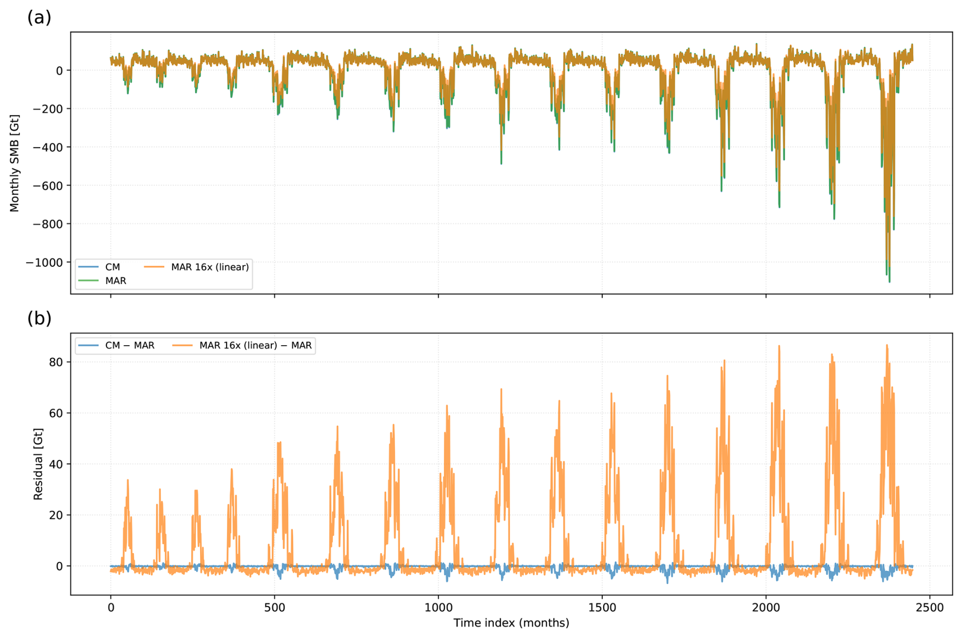
Figure 4 Monthly integrated SMB over test set for linearly interpolated SMB and downscaled field. (a) Monthly integrated SMB over the whole test set for MAR, CM and the linearly interpolated MAR field from the coarsened MAR field by a factor of 16. (b) Residuals between the downscaled field and the ground truth MAR and the linearly interpolated SMB field and MAR. The linearly interpolated fields overestimates the SMB compared to MAR during the melting seasons. The downscaled fields approximately conserve the SMB even for strong melt.

By enforcing hard conservation of the SMB and temperature during inference, the CM is able to generalize to more extreme climate conditions at the end of the training distribution without the need for retraining.

3.1.2 Determining optimal noising scale

To determine the optimal noising scale, we generate 50 different realizations for each month of the test set for different noising intensities and calculate the CRPS. We find that a noising time of t=10 results in the lowest CRPS of 5.37 $\mathrm{mm}\mathrm{w}.\mathrm{e}.$ per month (Fig. 5b), while also ensuring agreement with the high resolution power spectral density (Fig. 3). For noising scales larger than t=10, the CRPS converges to around 5.50 $\mathrm{mm}\mathrm{w}.\mathrm{e}.$ per month (Fig. 5e–g). The CRPS is generally largest at the margins, where the SMB variability is the largest and lowest in the interior with little variability. Similarly, the CRPS for the surface temperature is lowest for t>5 with CRPS=0.1 K (Fig. 5g).

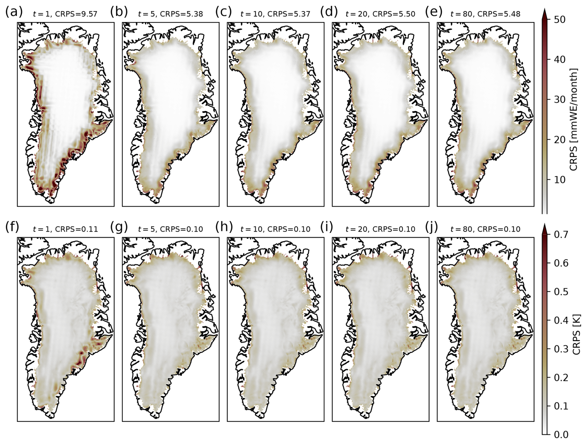
Figure 5 Continuous ranked probability scores (CRPS) for different noise scales over the test set for SMB and T_s. (a) Spatial mean CRPS for the noising time t=1. For each month of the test set, an ensemble of 50 realizations is generated and compared to the corresponding ground truth. The spatiotemporal mean CRPS is 9.57 $\mathrm{mm}\mathrm{w}.\mathrm{e}.$ per month. The CRPS is largest at the margins of the ice sheet, where the variability is largest. (b–e) Same as (a) but for different noising times. The noising time t=10 leads to the lowest CRPS. (f–j) Same as (a)–(e) but for the surface temperature. The CRPS converges to 0.1 K for t>10.

3.2 Downscaling ESM output

3.2.1 NorESM SSP-5.85

To show the application of our downscaling method, we directly downscale the approximated SMB (sum of precipitation, evaporation and runoff) of the NorESM2 output. The quality of the SMB field strongly depends on the ESM's ability to correctly simulate these variables. Most CMIP6 ESM's strongly overestimate the SMB or underestimate the melt in the higher emission scenarios. Hence, the SMB fields provided by the ESM's are not necessarily in accordance with the RCM simulations, even after bias correction (Fig. C1a–d). The (bias-corrected) temperature, on the other hand, reproduces the overall warming trend shown by MAR reasonably well (Fig. C1e–h).

We compare the downscaled fields to the MAR fields for the same scenario. For this downscaling exercise, we use the Norwegian ESM (NorESM2) (Seland et al., 2020) under the SSP-5.85 forcing scenario, in order to show the general applicability of the approach. We bias correct the fields before feeding into the CM. This correction is necessary since the original NorESM2 fields show a substantial bias, where the integrated yearly SMB is already negative in the historic period (Fig. 6a). After bias correction, the fields are in accordance with the historic MAR fields driven by ERA5. These fields are subsequently used as input into the CM.

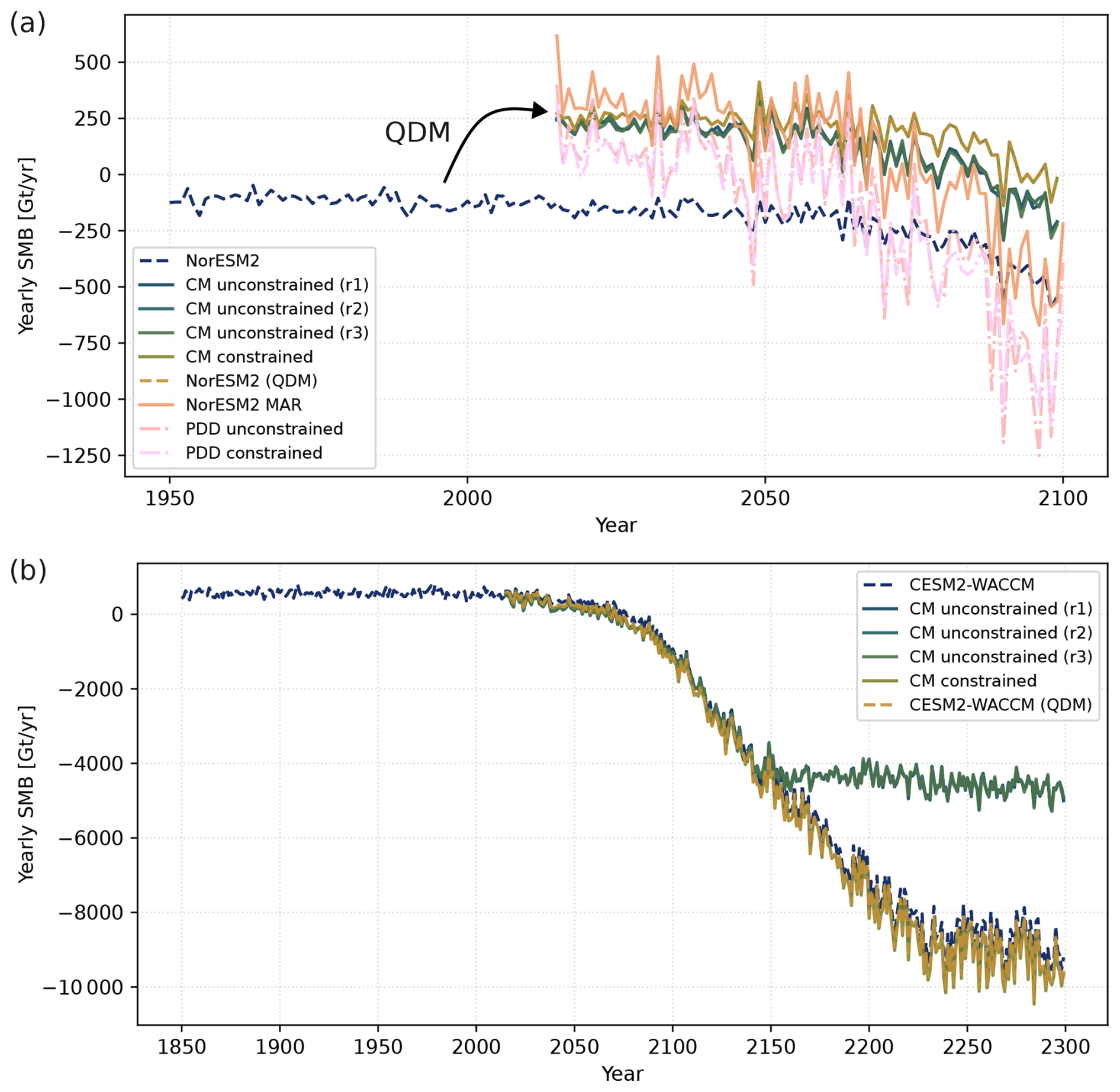
Figure 6 Integrated yearly SMB for NorESM2 SSP-5.85 and CESM2-WACCM SSP-5.85 scenarios. (a) Integrated surface mass balance from 1950 (2015) to 2100 for the NorESM2 model. We show the original integrated SMB over the whole ice sheet following the MAR mask derived from NorESM2 (dashed blue line), the bias corrected SMB using bias correction via QDM (dashed orange line), the downscaled SMB using the constrained CM (orange line), three realisations of the unconstrained downscaled fields (r1, r2, r3) and the corresponding MAR fields forced by NorESM2 (pink line). The MAR fields generally show a stronger trend in the SMB than the NorESM2 fields. (b) Similar to (a) but for CESM2-WACCM until the year 2300. The unconstrained realisations show a nearly constant SMB after the year 2150. The constrained CM downscaled field approximately conserves the SMB even for strong melt in the 23rd century.

While the CM is able to realistically downscale the SMB, the downscaled fields underestimate the melting season at the end of the century, i.e. show a higher SMB, compared to the corresponding MAR fields (Fig. C1c). This follows from the input fields, that is, the QDM-corrected SMB fields, which show the same patterns (Fig. C1b). This is also visible in the integrated yearly SMB over Greenland (Fig. 6a). The MAR run shows a 400–600 Gt yr⁻¹ smaller yearly SMB than the bias-corrected and downscaled NorESM2 fields at the end of the 21st century (Fig. 6a).

Per construction, the CM downscaling follows the large-scale patterns and hence cannot correct the low SMB if the input field show a low SMB bias. The MAE of the field downscaled by the CM is only slightly lower than that of the QDM-corrected field alone, but it effectively recovers the variability at small spatial scales (Figs. C1 and C2). If the bias-corrected fields show very sharp and large transitions between individual grid cells or simply show very unrealistic spatial SMB fields, the conservation of the SMB can lead to wrong values, where they are not expected since the CM is trying to conserve the overall SMB of the locally defined region (superblock). In other words, the constrained CM cannot simply correct fields that are spatially incoherent. An example of this behavior is shown in Fig. C3. The QDM-corrected field produces an unrealistically sharp transition from a high accumulation area with positive SMB at the southeastern margin to almost zero SMB (Fig. C3b). While the CM downscales to a realistic SMB at the southeastern margin, the CM then is forced to compensate with a slightly negative SMB west of the accumulation area due to the overall conservation of the SMB (Fig. C3c). To avoid this behavior, the input field can be linearly interpolated beforehand or the superblock size has to be tuned accordingly.

The original temperature fields are substantially too cold (Figs. C1e and C2e), while the bias corrected fields show a similar temperature range compared to the MAR fields (Figs. C1f and C2f). This shows the importance of bias-correcting ESM fields for any further analysis. The CM fields show the smallest MAE with 0.68 K for a random warm month and 0.72 K for a random cold month. Over the whole time period, the MAE of the downscaled SMB fields is 47.3 $\mathrm{mm}\mathrm{w}.\mathrm{e}.$ per month and for the temperature 1.17 K, compared to the MAR fields forced by NorESM2. The largest differences are at the southeastern and western margins (Fig. C4).

3.2.2 Hybrid PDD-model

Since the SMB simulated by the NorESM underestimates the melt at the end of this century, we show an additional approach using a simple SMB parameterisation. Specifically, we show how our approach can be used in a hybrid manner by (i) using a physically-motivated model to get a low-resolution estimate of the SMB and (ii) run the CM to get a high-resolution field from this estimate. We run a simple offline PDD model with the bias corrected NorESM2 (SSP-5.85) temperature field (ts) and the precipitation field (pr) as input to get a very simple estimate of the SMB. For simplicity, we do not bias correct the precipitation field before calculating the SMB, which might improve the SMB further.

The integrated yearly SMB of the PDD-derived SMB fields shows a similar trend as the MAR-forced-by-NorESM2 fields, but more pronounced (Fig. 6a). The SMB is 100–200 Gt yr⁻¹ lower than the MAR-forced-by-NorESM2 fields over the whole time period with some years showing 500 Gt yr⁻¹ lower SMB for the PDD fields (Fig. 6a). The unconstrained and constrained CM fields show relatively similar absolute SMB values. The interannual variability of the SMB is similar to the MAR fields and greater than for the bias-corrected NorESM2 fields (Fig. 6a).

We find a MAE of 32.6 $\mathrm{mm}\mathrm{w}.\mathrm{e}.$ per month over the whole time period and the MAE of the temperature remains 1.16 K (Fig. C5a and b). For comparison, the MAE of the non-downscaled PDD-derived SMB field is higher with 48.7 $\mathrm{mm}\mathrm{w}.\mathrm{e}.$ per month and 1.20 K for the temperature (Fig. C5c and d). Again, the margins show the largest error and the CM is able to recover the small-scale variability. While the PDD approach does not substantially improve the performance compared to the QDM approach, it shows that the CM can be used in a hybrid manner, i.e., using it in combination with a physics-based model.

3.2.3 Extreme climate until the year 2300 with CESM2-WACCM

To further test the generalizability of our approach, we downscale ESM output from the CESM2-WACCM model. We run the CM in the constrained and unconstrained mode to downscale the bias-corrected fields from a nominal resolution of 100 to 5 km resolution.

The integrated yearly SMB show a strong decrease after the year 2100 (Fig. 6b). The bias-corrected CESM2-WACCM SMB fields generally show a lower SMB than the non-bias-corrected fields over the whole time period (Fig. 6b). The constrained CM downscaled fields conserve the overall SMB and therefore the negative trend over the whole time period. The unconstrained realisations closely follow the integrated SMB of the bias-corrected fields until the year 2150 but then show a nearly constant SMB after the year 2150. This is because the unconstrained CM is not trained on SMB fields after the year 2100 and therefore is not able to reproduce the overall trend of more extreme climates. The unconstrained CM simply generates realistic fields based on the learned distribution. Interestingly, the unconstrained CM is nonetheless able to generate realistic fields for the extreme climate conditions until the year 2150 even though the CM was only trained on data until the year 2100. Even in the years after 2100, the unconstrained CM is able to generate realistic spatial patterns when the input fields are similar to the training data (Fig. D1).

We find that the constrained CM struggles to downscale spatial fields that are very different from the training data in terms of spatial coherence (Fig. D2). Similar to the NorESM2 case, the constrained CM cannot correct spatial patterns in the input fields that are very far from the learned spatial distributions due to the overall conservation of the SMB in each superblock. This leads to wrong SMB values in regions where they are not expected due to the overall conservation of the SMB in each superblock. This is especially pronounced in months where the negative SMB reaches further inland in the low-resolution model input than in the high-resolution training data. The CM then downscales the SMB to match the learned spatial distribution of the negative SMB at the margins and tries to uphold the conservation of the overall SMB by generating positive SMB values further inland within the superblock.

4 Discussion

4.1 Unconstrained versus constrained mode

We allow to run the CM in a constrained and unconstrained mode. Both modes have different advantages and disadvantages. While the constrained mode generally shows better performance in terms of MAE and correlation, it comes at the cost of reduced sample diversity. The CM is a probabilistic model that is able to generate multiple realistic samples for the same low-resolution input. However, the constrains reduce the ensemble spread and sample diversity. The constrained CM is forced to conserve the SMB on a regional level, which effectively reduces the degrees of freedom of the model and therefore the sample diversity. The noise strength is controlling the spread across the ensemble members and the pairing strength with the initial input.

Interestingly, we find that the unconstrained mode shows better performance for some months (compared with the MAR ground truth) that are not outside of the training distribution, i.e. before the year 2100. This is due to the fact that the unconstrained CM has more freedom to generate realistic fields without being forced to conserve the SMB on a regional level. The local conservation constrains the degrees of freedom that allow for generating realistic spatial patterns.

For extreme future climates with very negative SMB fields at the end of the century and beyond, the constrained CM usually shows better performance than the unconstrained CM (Fig. 6b). This is because the unconstrained CM is not trained on such extreme SMB fields and therefore cannot reproduce the overall trend toward more negative SMB. This is clearly visible in the integrated downscaled SMB of CESM2-WACCM after the year 2150, where the unconstrained CM yields a nearly constant SMB (Fig. 6b), effectively plateauing at the lower end of its learned SMB distribution.

The approach of constraining the model via mass conservation generally assumes confidence in the overall low-resolution SMB fields but it allows generalization to more extreme or even out-of-sample SMB fields without the need of retraining the CM. This could be used to downscale regional climate models when running on a high-resolution grid is too expensive or time consuming. The subsequent downscaling step with the CM ensures conservation of the overall SMB fields and trend while providing realistic high-resolution fields at the same time. However, it should be noted that the constrained CM is not able to provide realistic downscaled fields if the input is very different from the training data in terms of spatial coherence (Fig. C3). This can lead to incorrect SMB values in regions where they are not expected due to the overall conservation of the SMB in each superblock. This is especially pronounced in months where the negative SMB reaches further inland in the low-resolution model input than in the high-resolution training data. The CM then downscales the SMB to match the learned spatial distribution of the negative SMB at the margins and tries to uphold the conservation of the overall SMB by generating positive SMB values further inland within the superblock. We find that this behavior can partially be mitigated by not using the region-growing algorithm, using smaller superblocks or reducing the smoothing of the residuals before applying the constraint. However, there is a tradeoff between these choices and generating realistic spatial small-scale patterns. By extending the training data with more extreme fields beyond the year 2100 based on RCM simulations, this problem could be mitigated.

Alternatively, the unconstrained CM can be used to generate unconditional samples that represent constant present-day forcing with the learned natural variability. This can be used for, e.g., spinup simulations, when a constant climate with variability is desirable. Another advantage of the hard-constrained mode is in the context of embedding downscaling approaches within existing process-based models such as ESMs. In ESMs, conservation of, for example, water, mass and energy is important to enforce physical consistency between the individual components. Our constraining approach ensures conservation of these variables, while allowing higher resolution.

It should be noted, that our constraining approach is relatively simple and can be improved by, for example, incorporating the constraint layer directly into the network architecture, using a different constraint approach (Harder et al., 2023) or by simply improving our region-growing algorithm, which might fail for some special cases. We also tried multiplicative constraints during inference (not shown). However, we found that this approach leads to artifacts during the sampling process. Specifically, very high or very low SMB values in random regions.

4.2 Training data dependency and technical limitations

Due to the nature of data-driven approaches, our results are strongly dependent on the quality of the training data. Here, we only use the regional climate model MAR, however, additional regional climate models such as RACMO (van Dalum et al., 2024) are available. It has been shown, that these show variations by a factor of two in future projections of the SMB (Glaude et al., 2024). Naturally, our downscaled fields are therefore biased towards the MAR projections. Including additional RCMs during training could help to reduce this model dependency and also lead to more generalizability of the CM to different spatial fields. Nonetheless, our constraining approach overcomes this problem to some extent by enforcing approximate conservation of the regional SMB.

Unlike precipitation, which is defined (even if zero) everywhere and can be treated as a spatially continuous field, surface mass balance is strictly confined to the ice-sheet mask. Downscaling SMB, therefore, must handle sharp domain boundaries at the ice edge, where values abruptly drop to zero, rather than the smooth transitions typical of precipitation fields This leads to several technical challenges on how to treat the outside of the ice sheet in spatially-aware generative models. We decided to simply treat the SMB outside the ice sheet as zero. In the case of a non-evolving topography, as given by the training data, this is the most natural choice. However, this also means that our model is currently restricted to ice sheet geometries that do not extend beyond present-day extent due to the nature of the training data. With increasing availability of high-resolution RCM simulations with evolving topography this problem might be solved (Delhasse et al., 2024; Paice et al., 2026). Similarly, the resolution of the output field is mostly limited by the training data. Training data with even higher resolution would also allow to generate even higher resolution downscaled fields. However, for very high resolutions, the training might be limited by the available GPU memory.

4.3 Generalizability

We have shown that our physics-constrained CM is able to realistically downscale SMB and surface temperature fields of the GrIS from low-resolution input fields by a factor of up to 32, independent of the low-resolution source. Beyond a factor of 32, we find that the CM reaches its limit and does not provide reasonable fields.

Our approach is in principle not limited to the GrIS and can be applied to other ice sheets such as Antarctica or glaciers as well. However, retraining of the CM is necessary due to the different climate and SMB characteristics. By nature, our model requires high-quality training data that resolves the small-scale variability of the SMB and T_s fields, which might not be available in the necessary quantity for Antarctica. We find that the CM needs a minimum number of 10 000–15 000 training samples to be able to generate realistic spatial fields. This effectively corresponds to approximately 830–1250 years of monthly data. Generating these amounts of data with RCMs is computationally expensive and time consuming, and to our knowledge not available for Antarctica at the moment.

4.4 Towards a full ML-based SMB model

Our approach uses as a conditional generative model that learns to sample from a distribution of realistic high‑resolution SMB fields given coarse inputs rather than a deterministic classical regression that predicts the SMB from external input such as the temperature or precipitation. As in any downscaling task, our recovered SMB and T_s fields strongly depend on the quality of the low-resolution input fields, that is, the ability of the ESM or physics-based model to accurately simulate the SMB and T_s at the coarse scale. We tried including the temperature as additional input to the CM during training (i.e., predictor) for the SMB (not shown). While we were able to generate realistic samples, the warming trend and interannual variations were underestimated in future emission scenarios.

A more promising alternative approach would be to separate the regression, i.e., predicting SMB from ESM variables, and downscaling tasks (Aich et al., 2025). For example, a U-net could be trained to learn a regression from several input variables to give a first low-resolution estimate of the SMB with subsequent downscaling using the CM. Depending on the chosen regressor variables such an approach would allow a coupling with an external ice sheet model and therefore a first prototype of a hybrid SMB–ice sheet model. Alternatively, the CM could be used to directly downscale, for example, precipitation, runoff and evaporation fields from the ESM instead of the SMB. The CM model we present here is therefore a first step in this direction.

5 Conclusion

This study introduces a physics-constrained generative machine learning approach, based on consistency models to downscale the spatial SMB and T_s fields of the GrIS. We train our model on the regional climate model MARv3.12 and show that our approach is able to downscale the SMB and T_s fields by a factor of up to 32, from 160 km resolution to 5 km resolution in an efficient and realistic manner. The resulting fields are visually similar to the ground truth and the CM is able to successfully recover the small-scale variability of the SMB and T_s fields. Furthermore, we show how our model can be used to directly derive high-resolution SMB and T_s fields from the ESM by combining the CM with either (i) a bias-correction method (QDM) or (ii) a physics-based method (PDD).

Our approach is a first step towards a more general machine-learning driven SMB model. An application of our approach to Antarctica is straightforward but likely needs retraining and corresponding high-quality training data. Alternatively, our approach could be integrated into ESMs either to downscale SMB fields provided by the land component or to directly downscale precipitation fields. Usually, the resolution of the precipitation fields generated by the atmospheric component is several times lower than the native resolution of the ice sheet model. Hence, the precipitation does not resolve the topography of the ice sheets at all, which in turn leads to unrealistic spatial precipitation distribution and ultimately SMB. Using the CM with hard-constraints to downscale the precipitation fields during runtime could solve this problem. Overall, generative modeling is a promising approach to downscale arbitrary climate fields in computationally fast manner.

Appendix A: Unconditional samples

To show that our models correctly learn the distribution of the underlying training data, we generate 100 unconditional SMB samples for each month and compare them to the training set (Fig. A1). While, the SMB modeled by MAR is not a ground truth in the classical sense, we treat it as such in lack of observational SMB fields and refer to it as such in the following. Here, we refer to unconditional samples as samples that are generated from noise, i.e., without any initial guesses of the SMB. However, these samples are conditioned on the auxiliary inputs, i.e., the ice sheet height and insolation.

The CM is able to generate realistic unconditional SMB field samples, both for the winter and summer season (Fig. A1a and b). The mean and standard deviation of the generated set closely follow the mean and standard deviation of the training set, except for the summer season (Fig. A1h–j). In all summer months (JJA), the average SMB is greater than the corresponding training set mean SMB. Similarly, the standard deviation of the generated ensemble is smaller. This is almost exclusively due to the greater SMB at the margins in the generated ensemble. In other words, the generated ensemble underestimates the melt and variability of the SMB at the ice-sheet margins in the summer months. Interestingly, the generated ensemble mean SMB in May is smaller and the variability is greater than that of the training set (Fig. A1g).

Generally, we are not interested in generating unconditional samples. Therefore, the overestimation of the SMB at the margins in the summer months is not a problem for the downscaling task per-se. We overcome this problem by introducing a hard constraint that conserves the SMB from the low-resolution fields on a regional scale. We find, that the hard-constraining generally improves the results.

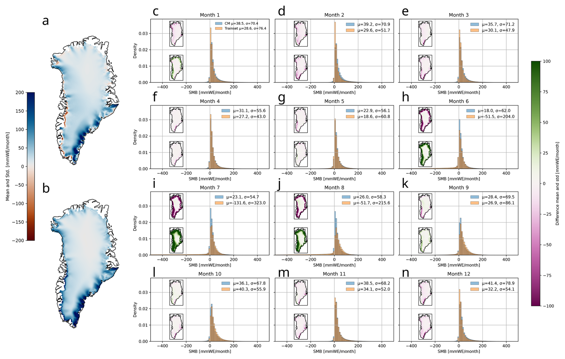
Figure A1 Unconditional sampling of SMB from trained CM. (a) Mean surface mass balance over unconditional sample set. (b) Same as (a) but for the standard deviation. (c) Histogram of the generated SMB samples and the training set for January. The mean and standard deviation of each set are denoted. The inset shows the spatial difference of the mean (top) and standard deviation (bottom) between the generated samples and the training set. Green corresponds to areas where the CM samples have a smaller mean/standard deviation, while pink areas denote regions where the CM has a larger mean/standard deviation than the training set. (d–n) Same as (a) but for all other months of the year. The CM is mostly reproducing the mean and standard deviation well but overestimates the SMB in the summer months with strongly negative SMB.

Appendix B: Examples of downscaled fields

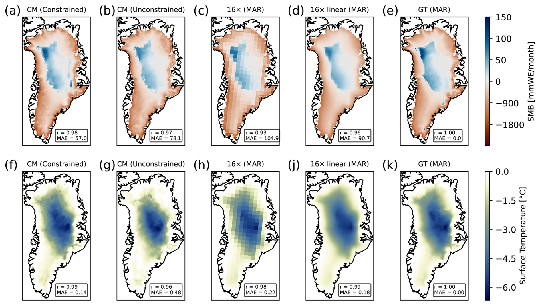
Figure B1 Exemplary downscaling of surface mass balance and temperature at surface for random month from test set. (a) Downscaled SMB field of the test set with hard constraints during inference for a warm month with negative SMB at the margins (red) with a 5 km resolution. The mean absolute error (in $\mathrm{mm}\mathrm{w}.\mathrm{e}.$ per month) and Pearson correlation with the ground truth field are denoted. (b) Same as a but for the unconstrained CM. (c) We show the coarsened MAR field by a factor of 16 (80 km resolution), which is the input for the CM. The small scale variability is lost. (d) Same as (b) but linearly interpolated. (e) Ground truth MAR field with a 5 km resolution. (f–j) Same as (a)–(e) but for the surface temperature.

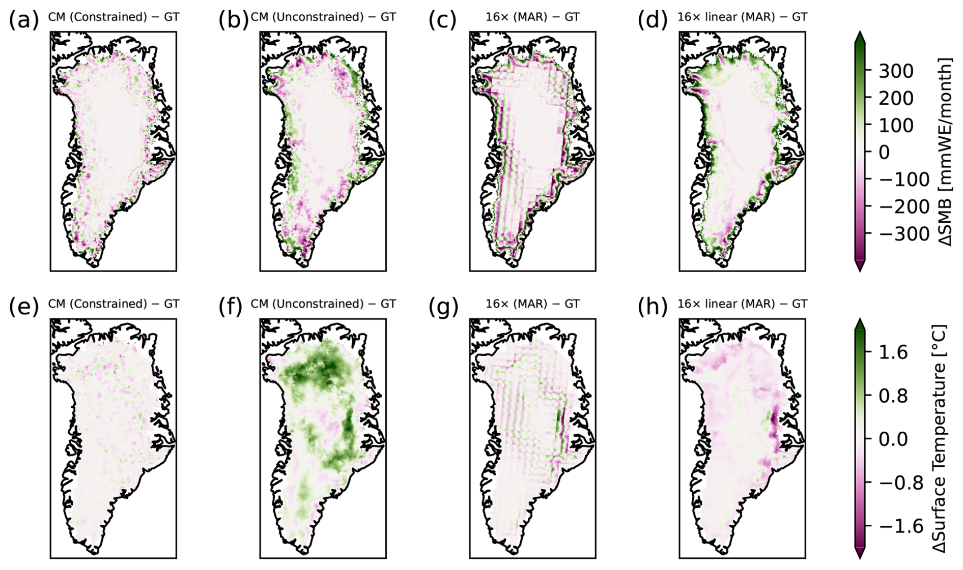
Figure B2 Difference between downscaled fields and MAR of surface mass balance and temperature at surface for random month from test set. (a) Difference between downscaled SMB field using the constrained CM and MAR for same random month as shown in Fig. 3. (b–d) Same as (a) but for the unconstrained CM, the pooled SMB field and the linearly interpolated SMB field, respectively. (e–h) Same as (a)–(d) but for the temperature at surface. The constrained CM generally shows the smallest residuals compared to MAR.

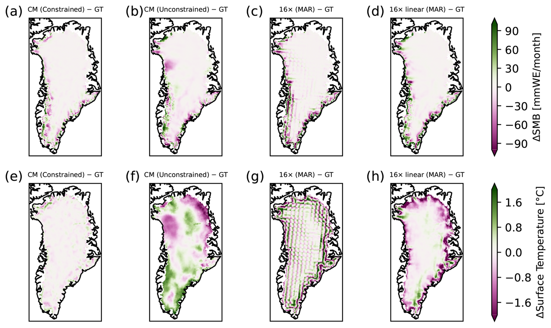
Figure B3 Difference between downscaled fields and MAR of surface mass balance and temperature at surface for random month from test set. (a) Difference between downscaled SMB field using the constrained CM and MAR for same random month as shown in Fig. 3. (b–d) Same as (a) but for the unconstrained CM, the pooled SMB field and the linearly interpolated SMB field, respectively. (e–h) Same as (a)–(d) but for the temperature at surface. The constrained CM generally shows the smallest residuals compared to MAR.

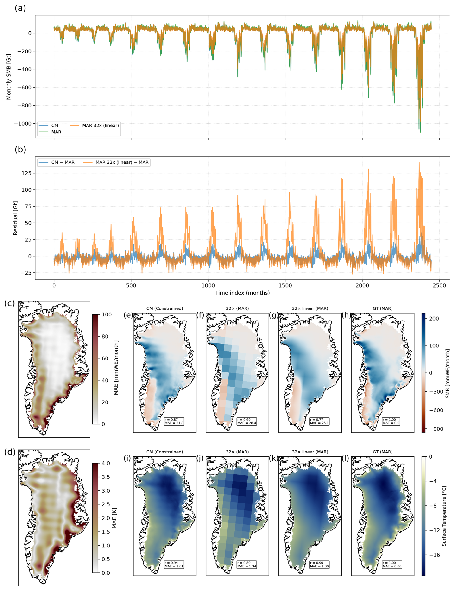
Figure B4 Downscaling of coarsened MAR test set by factor 32. (a) Monthly integrated SMB over whole test set for MAR, CM and linearly interpolated MAR field from the coarsened MAR field by a factor of 32. (b) Residuals between downscaled field and ground truth MAR and linearly interpolated SMB field and MAR. The linearly interpolated fields overestimates the SMB compared to MAR during the melting seasons. While the downscaled fields also over- and underestimate the SMB they show substantially smaller residuals compared to the linearly interpolated fields. (c) MAE of downscaled SMB fields over whole test set. The coarse structure of the input field is still partially visible in the MAE field. The average MAE over the whole test set is 24.6 $\mathrm{mm}\mathrm{w}.\mathrm{e}.$ per month. (d) Same as (c) but for surface temperature. The MAE over the whole test set is 1.35 K. (e) Downscaled SMB field of test set with hard constraints during inference for a warm month with negative SMB at the margins (blue) with a 5 km resolution. The mean absolute error (in $\mathrm{mm}\mathrm{w}.\mathrm{e}.$ per month) and Pearson correlation with the GT field are denoted. (b) Coarsened MAR field by a factor of 32 (160 km resolution), which is the input for the CM. The small scale variability is lost. (d) Same as (b) but linearly interpolated. (e) Ground truth MAR field with 5 km resolution. (f–j) Same as (e)–(h) but for the surface temperature.

Appendix C: NorESM2 downscaling

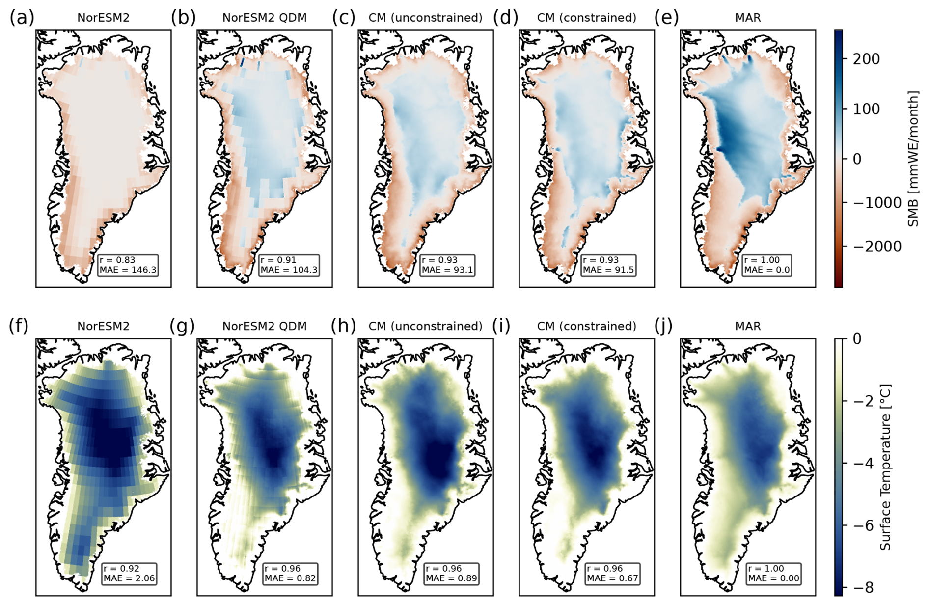
Figure C1 Exemplary downscaling of surface mass balance and temperature at surface for end of century month for NorESM2 SMB. (a) NorESM2 SMB as sum of precipitation, runoff and evaporation. The MAE and correlation compared to the (unpaired) MAR SMB for the same month are denoted. (b) QDM-corrected NorESM2 SMB. The margins show a more negative SMB compared to non-bias corrected SMB and positive SMB in the interior of the ice sheet. However, the SMB is still underestimated compared to the MAR SMB. (c) Downscaled SMB field with the unconstrained CM model to 5 km resolution. (d) Downscaled SMB field with the constrained CM model to 5 km resolution. (e) Unpaired high-resolution ground truth (GT) for this individual month as simulated by MAR. (f–j) Same as (a)–(e) but for the temperature at surface. The bias-corrected and downscaled T_s show stronger similarity with MAR than the SMB fields.

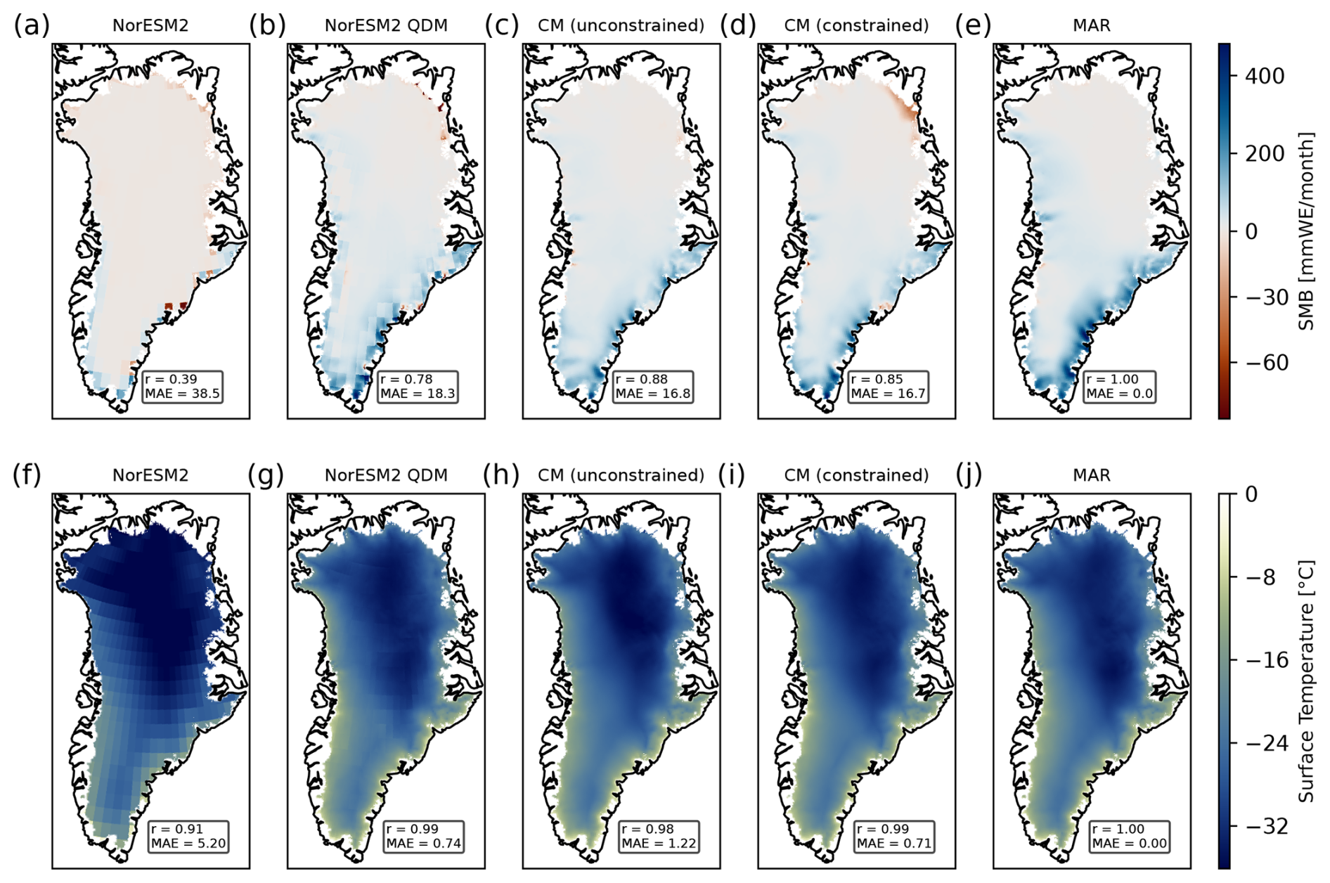
Figure C2 Exemplary downscaling of surface mass balance and temperature at surface for random month from test set (NorESM2). (a) NorESM2 SMB as sum of precipitation, runoff and evaporation. The MAE and correlation compared to the (unpaired) MAR SMB for the same month are denoted. (b) QDM-corrected NorESM2 SMB. The overall SMB is more positive than the non-biased corrected SMB. (c) The downscaled SMB field with the unconstrained CM model to 5 km resolution. (d) Same as (c) but with the constrained CM model. (e) Unpaired high-resolution ground truth (GT) for this individual month as simulated by MAR. (f–j) Same as (a)–(e) but for the temperature at surface.

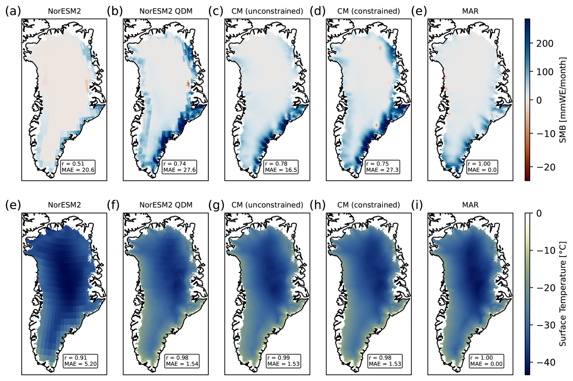
Figure C3 Exemplary downscaling of surface mass balance and temperature at surface for random month from test set with artifacts (NorESM2). (a) NorESM2 SMB as sum of precipitation, runoff and evaporation. The MAE and correlation compared to the (unpaired) MAR SMB for the same month are denoted. (b) QDM-corrected NorESM2 SMB. The SMB in the at the margins is substantially more positive than the non-biased corrected SMB. (c) The downscaled SMB field with the unconstrained CM model to 5 km resolution. (d) Same as (c) but with the constrained CM model. The unconstrained fields show better correspondence with the MAR SMB than the constrained CM fields in terms of the correlation and MAE. Artificats are visible (red area in southeastern part of the ice sheet) stemming from the CM trying to enforce conservation of the overall SMB in the respective region. (e) Unpaired high-resolution ground truth (GT) for this individual month as simulated by MAR. (f–j) Same as (a)–(e) but for the temperature at surface.

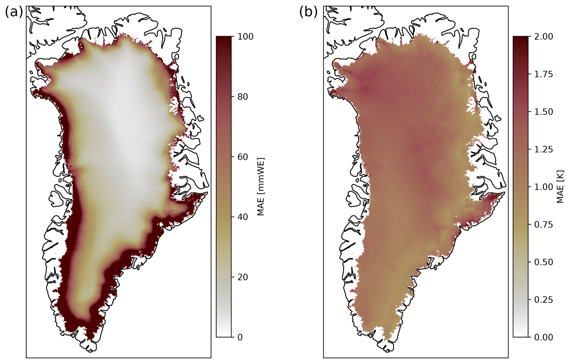
Figure C4 Mean absolute error over whole time period (2015–2100) for QDM-corrected NorESM2 SMB for SSP-5.85 scenario. (a) Temporal MAE for each grid cell of downscaled SMB from bias-corrected SMB field derived from NorESM2 SSP-5.85 run. The margins show the largest error. The spatial average mean absolute error is 47.3 $\mathrm{mm}\mathrm{w}.\mathrm{e}.$ per month. (b) Same as (a) but for surface temperature. The spatial average mean absolute error is 1.17 K.

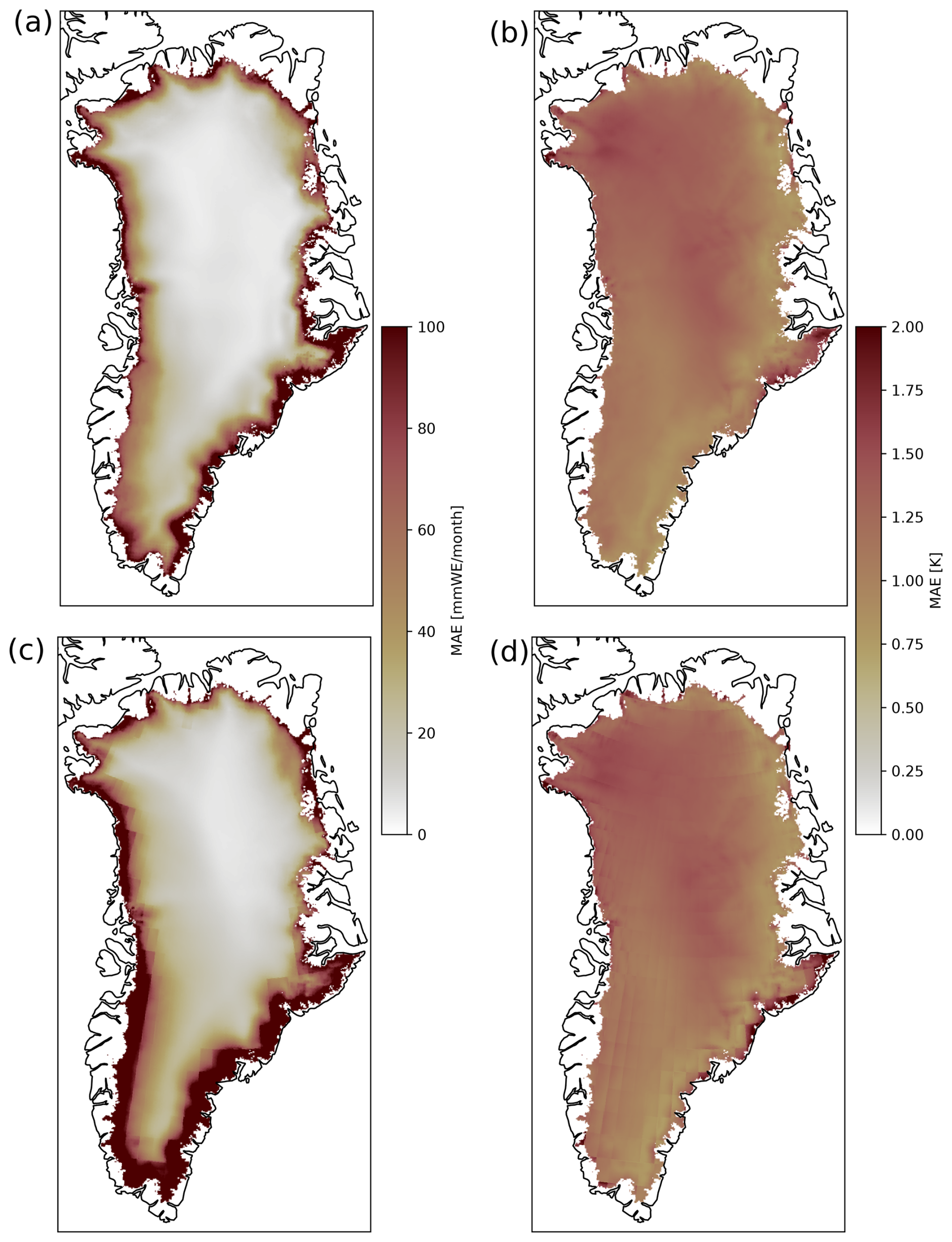
Figure C5 Mean absolute error over whole time period (2015–2100) for PDD NorESM2 SMB for SSP-5.85 scenario. (a) Temporal MAE for each grid cell of downscaled SMB from bias-corrected PDD derived SMB field forced by NorESM2 SSP-5.85 run. The margins show the largest error. (b) Same as (a) but for surface temperature. (c, d) Same as (a), (b) but directly for bias corrected SMB and T_s fields without downscaling.

Appendix D: CESM2-WACCM downscaling

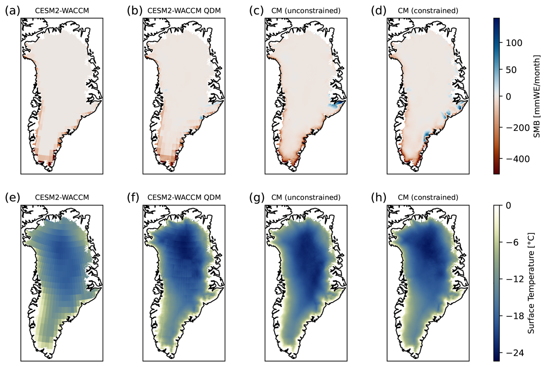
Figure D1 Exemplary downscaling of surface mass balance and temperature at surface for winter month in the year 2264 (CESM2-WACCM). (a) We show the CESM2-WACCM SMB in February 2264. (b) QDM-corrected CESM2-WACCM SMB. (c) The downscaled SMB field with the unconstrained CM model to 5 km resolution. (d) Same as (c) but with the constrained CM model. Both, the constrained and unconstrained CM show similar fields since the input SMB shows a similar spatial coherence than the training data set. (e–h) Same as (a)–(d) but for the temperature at surface.

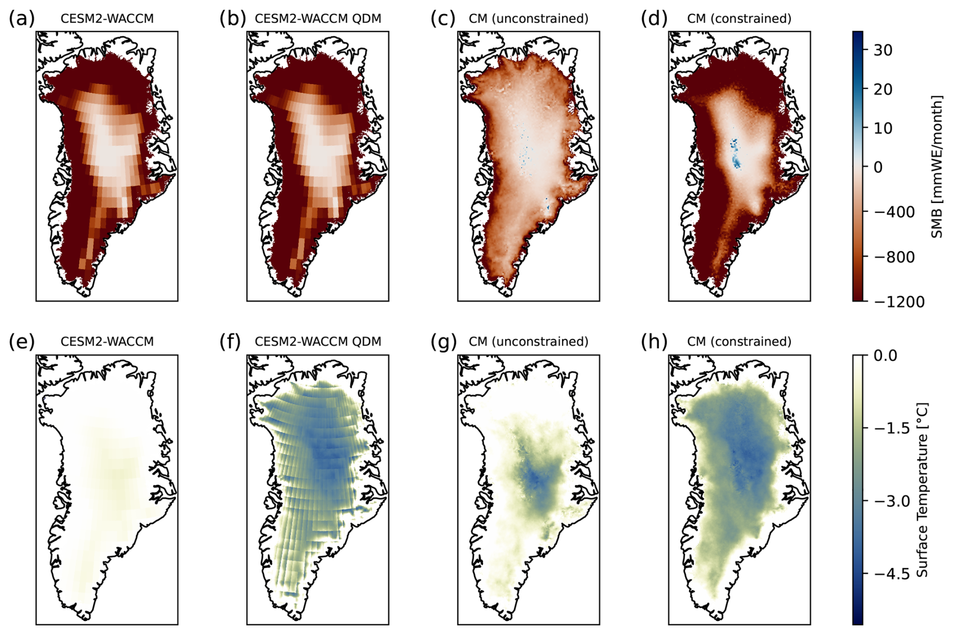
Figure D2 Exemplary downscaling of surface mass balance and temperature at surface for May 2264 (CESM2-WACCM). (a) We show the CESM2-WACCM SMB in May 2264. The whole ice sheet shows a negative SMB. (b) QDM-corrected CESM2-WACCM SMB. (c) The downscaled SMB field with the unconstrained CM model to 5 km resolution. The strong negative SMB values are not reproduced. The CM overesimates the SMB compared to the input field. (d) Same as (c) but with the constrained CM model. The constrained CM conserves the negative SMB but shows a region with positive SMB in the interior due to the conservation. (e–h) Same as (a)–(d) but for the temperature at surface.

Appendix E: Training and validation loss

Figure E1 Validation and training loss of consistency model.