Challenges in identifying Antarctic coastal polynyas in satellite observations and climate model output to support ecological climate change research

Antarctic coastal polynyas are key components of Antarctic marine ecosystems, influencing light and nutrient availability and open water access for marine predators. Thus, changes in the physical characteristics of polynyas can influence how these ecosystems respond to a changing climate. Here, we explore challenges inherent in identifying climatologically and biologically relevant Antarctic coastal polynyas on gridded data in both satellite and Earth System Model data. We find that it is critical to consider grid type and resolution, season, metric and threshold when defining polynyas. Regridding data, both spatially and temporally, can have significant impacts on identified polynya statistics. The spatial distributions of Antarctic coastal polynyas are significantly correlated between the two observational products as well as between the observational products and the model data. The Earth System Model we use here captures coastal polynya-like features that occupy ∼ 3 % of the area of the winter sea ice zone and contribute ∼ 17 %–21 % of the total sea ice zone marine net primary productivity (NPP). Temporal self- and cross correlations of integrated polynya areas and numbers are inconsistent across observational and modelling products. Trends in polynya areas are not robust, changing significance, magnitude and sign across threshold, grid and product.

1 Introduction

Polynyas, defined by the World Meteorological Organization as “any non-linear shaped opening enclosed in ice” and “may contain brash ice and/or be covered with new ice, nilas, or young ice” (World Meteorological Organization, 1970), can be found in the southern ocean both in open water and along the Antarctic coast. Open water polynyas are created when relatively warm ocean water upwells to the surface thermodynamically melting sea ice (“sensible heat polynyas”) – these are relatively uncommon and will not be discussed further in this work. Coastal polynyas are driven by cold downslope winds off the Antarctic continent that mechanically push sea ice away from the coast leaving open ocean water that rapidly loses heat and freezes into more sea ice (“latent heat polynyas”). Many coastal polynyas, particularly in Eastern Antarctic, are associated with land fast ice and grounded icebergs which influence the location and size of the polynyas formed through blocking ice advection (e.g. Fraser et al., 2019; Nihashi and Ohshima, 2015). Coastal polynyas occupy only a small area within the Southern Hemisphere sea ice zone yet play an outsized role in Antarctic sea ice production, deep water formation, global thermohaline circulation, carbon sequestration, and biological activity. Coastal polynyas produce about 10 % of the total Antarctic sea ice (Tamura et al., 2008) and one polynya alone – the Cape Darnley polynya produces ∼6 %–13 % of the total Antarctic Bottom Water (Ohshima et al., 2013). As regions of lower sea ice concentration and/or thinner sea ice, polynyas are the first oceanic regions within the sea ice zone exposed to light in the Antarctic spring. As a result, polynyas show enhanced production within the Antarctic sea ice zone, where phytoplankton growth tends to be limited by light (Arrigo and van Dijken, 2003; Arrigo et al., 2015) and spring phytoplankton blooms within polynyas are frequently synchronized with light availability (e.g. Li et al., 2016). Polynyas also provide Antarctic predators (e.g., penguins, seals) both open water access and augmented prey resources, with ephemeral polynyas being of particular importance for Emperor penguins (Labrousse et al., 2019). Coastal polynyas are sometimes referred to both as “polynyas” (indicating formation in the ice-growth season) and “post-polynyas” (formation in the melt season by the rapid melting of the relatively thin sea ice), in recognition of their important biological functions even when they may cease to be defined as “polynyas” in the strict definition (e.g. Arrigo and van Dijken, 2003; Criscitiello et al., 2013).

How Antarctic marine ecosystems respond to a changing climate will be determined, at least in part, by changes in the sea icescape, including the size, location and timing of coastal polynyas. Antarctic polynyas are formed within the sea ice zone, and the sea ice around Antarctica has been studied extensively using both satellite and Earth system model (ESM) data. Satellite observations of sea ice (1979–present) show small positive trends in Antarctic sea ice area (the total area of sea-ice) and extent (defined as the area covered by sea ice concentrations of 15 % or higher) until 2016 followed by unprecedented sea ice losses accompanied by changes in both persistence and variability (e.g., Fogt et al., 2022; Parkinson, 2019; Purich and Doddridge, 2023; Raphael and Handcock, 2022; Raphael et al., 2025; Turner et al., 2017, 2022). The most current ESMs contributing to the Climate Model Intercomparison Project phase 6 (CMIP6; Eyring et al., 2016) show a wide range of Antarctic sea ice states (e.g. Roach et al., 2020). Even though many ESMs capture the climatology of observed Antarctic sea ice, ESMs struggle to capture both the small, but significant, positive trend observed 1979–2015, and the more recent dramatic sea ice losses (Diamond et al., 2024; Roach et al., 2020). The recent, extreme losses and extended reconstructions of Antarctic sea ice suggest that there may be internal variability not captured by the relatively short observational record (e.g. Fogt et al., 2022; Hobbs et al., 2024; Holmes et al., 2024, and references therein). These assessments of Antarctic sea ice, however, focus predominantly on large-scale sea ice extent and area rather than the complex icescape within the ice pack where polynyas form.

Polynyas and polynya-like features often have scales and dimensions much smaller than those resolved by either satellite observations or global climate model data. For example, the median sizes of wintertime Antarctic coastal polynyas identified as key contributors to Antarctic primary production (e.g. Arrigo et al., 2015; Arrigo and van Dijken, 2003) and sea ice production (e.g. Tamura et al., 2008; Nihashi and Ohshima, 2015; Tamura et al., 2016) range from ∼1.3–6×10³ km², and many of these polynyas are relatively narrow (10–100 km). Thus, many of these biophysically critical polynyas cannot be resolved on the 25×25 km grid of the passive microwave satellite data (e.g. Special Sensor Microwave Imager [SSM/I]), much less on the typically coarser ∼1° ($\sim \mathrm{100}\times \mathrm{100}$ km) resolution ESM grids. The challenge of identifying relatively smaller polynyas on relatively coarser grids has been explored in observational data products with a polynya signature simulation method (PSSM; Markus and Burns, 1993), which combines higher resolution 85 Ghz frequency data with the high contrast data of the 37Ghz channel to classify SSM/I data as shelf ice, open water or sea ice (rather than SICs) and from which polynya maps can then be created at sub-pixel scales. This method has been applied to studies of marine productivity in Antarctic coastal polynyas (e.g. Arrigo and van Dijken, 2003; Arrigo et al., 2015). Tamura et al. (2006, 2007) address the resolution problem by combining SSM/I with the advanced very high-resolution radiometer data (AVHRR) to estimate sub-grid scale sea ice thickness (SIT) in regions of thin sea ice. The resulting maps of sea ice thicknesses in thin sea ice areas along with reanalysis data from both the European Centre for Medium-Range Weather Forecasts (ERA-40) and the National Centers for Environmental Prediction (NCEP2) were used to make maps of sea ice production and variability in Antarctic polynyas (Tamura et al., 2007, 2016). This method of identifying thin sea ice areas was applied in work investigating the influence of icescapes on Emperor penguin foraging habitat in East Antarctica (Labrousse et al., 2019).

The PSSM and sea ice production methods have been successfully used in identifying polynyas at sub-pixel scales in the satellite data, yet they are not directly applicable to ESM data which is saved as grid-cell averaged quantities. Polynya studies using ESMs thus use grid-cell averaged sea ice concentration (SIC) and/or thickness (SIT) thresholds to identify “polynya” grid cells of lower and/or thinner sea ice than the surrounding grid cells (e.g. Mohrmann et al., 2021; DuVivier et al., 2024) – a method that has also been applied to satellite-based SICs (e.g. Massom et al., 1998; Duffy et al., 2024). These low sea ice grid cells are then labelled polynyas, although strictly speaking they identify grid cells that have a polynya-like feature within them per the given threshold rather than explicitly resolving individual polynya(s) within the grid cell. September Antarctic polynya areas in CMIP6 models identified by SICs and SITs show particularly large inter-model spread in size and frequency across all CMIP6 models, and differences in coastal polynyas are attributed at least in part to differences in horizontal resolution although the impacts of different resolutions have not, to our knowledge, been explored (Mohrmann et al., 2021). ESMs compute sea ice production directly, which in turn can identify regions of high-sea ice productivity and thus infer coastal polynya regions – although resolution of these regions will still depend on the model grid (e.g. Jeong et al., 2023).

Satellite data and ESM output have different methodologies for determining SICs, which further complicate comparisons of polynyas and/or polynya-like features identified in these products. Satellite SICs are retrieved from satellite microwave radiometers using sea ice algorithms which differ in their sensitivity to sea ice temperature and emissivity, atmospheric conditions (including winds, cloud liquid water vapor content, humidity), surface roughness in open water areas and the sea ice state and presence of liquid water on the sea ice (e.g. melt ponds). Uncertainties in satellite-based SICs tend to be greatest in summer season, and regions of low sea ice concentrations and thin ice (e.g. Meier et al., 2021b; Ivanova et al., 2015, and references therein). Earth system model SICs, on the other hand, are based on the physical evolution of simulated sea ice due to fluxes of energy and momentum. ESMs calculate SICs/SITs to very small fractions/thicknesses, albeit with potential biases from forcing or structural model uncertainty. Most ESMs use an ice thickness distribution (ITD) to represent the heterogeneity of sea ice thicknesses within a grid cell. The average sea ice thickness of a grid cell is calculated as the total volume of sea ice in the discrete thickness categories divided by the area of the grid cell. Satellite-derived SIT estimates are becoming more readily available, yet remain spatially and temporally limited compared to SICs, particularly in the Antarctic, and have considerable uncertainty compared with SIC products (e.g. Bocquet et al., 2024; Fons et al., 2023; Kacimi and Kwok, 2022; Zygmuntowska et al., 2014, and references therein). Thus, SIT from satellite products has limited capacity for identifying thin sea ice which may be relevant for polynyas, especially during the active ice-growth period of wintertime coastal polynyas. Further, ESM SICs and SITs are calculated at the model time-step (e.g. every hour) then averaged over a day for daily averages, whereas satellite microwave radiometer data represent an instantaneous snapshot of conditions specific to a particular time and location (typically daily or bi-daily; Meier et al., 2014).

ESMs are powerful tools for exploring past, present and future climates and how polar marine ecosystems may respond to climatic change, and satellite SIC data have been used extensively to validate sea ice areas and extents in ESMs. Earth system models (ESMs) are increasingly being used to study polynyas in the climate system (e.g. Mohrmann et al., 2021; Jeong et al., 2023; DuVivier et al., 2024) yet we are unaware of any publications that assess in detail how to best identify and compare climatologically relevant polynya-like features in both ESMs and satellite products. The following are the four primary questions we address in this work:

1. Are Earth System Models (ESMs) capable of capturing climatologically and biologically relevant coastal polynya-like features?

2. How to best use observational products to validate polynya-like features in ESMs?

3. Do polynya-like features in ESMs forced by reanalysis data occur in regions/areas where polynyas and polynya-like features are identified in observations?

4. Do coastal polynya features in ESMs function in marine ecological processes as they do in the real world?

We also seek to understand how choice of polynya metrics may influence results in terms of polynya areas, locations and trends. We intend for this exploration to give guidance on implications of various polynya metric choices for model and satellite-based data analysis. The role of low sea ice areas in Antarctic marine ecosystems is dynamic and diverse – polynyas affect availability of light and nutrients for phytoplankton, provide open water access and thus prey for marine predators such as penguins and seals, and the timing of low sea ice conditions influences the seasonal progression of phytoplankton blooms. In this paper, we investigate the impacts of metric choices on coastal polynya identification, compare polynya areas estimated from simulated and observationally based data, and assess if our polynya metrics identify biologically important marine regions in the climate model. This analysis provides comprehensive and quantifiable information on polynya identification that can help guide future work to assess the role of changing polynyas on Antarctic marine ecosystem dynamics and the physical environment.

2 Data

2.1 Satellite observations

We consider two daily observational Climate Data Records (CDR) of gridded sea ice concentration data from satellite images: version 4 of the CDR of passive microwave SIC developed at the National Snow and Ice Data Center (NSIDC) for the National Oceanic and Atmospheric Administration (NOAA; Meier et al., 2014, 2021a) and the European Organisation for the Exploitation of Meteorological Satellites (EUMETSAT) Ocean and Sea Ice Satellite Application Facility (OSISAF) SIC CDR (OSI-450) from 1979–2015 and the OSI-430-b from 2016–2020 (Lavergne et al., 2019). The NOAA data are a merged product of the NASA Team (Cavalieri et al., 1984) and Bootstrap (Comiso, 1986; Comiso et al., 1997) algorithms, with the higher SIC of the two products used as the CDR value when the two products differ (Meier et al., 2014). The NOAA and OSISAF data are derived from the same satellite radiometer data using different sea ice retrieval algorithms. The largest differences in SICs resulting from different retrieval algorithms tend to be found in areas of relatively thin sea ice, where SIC tend to be underestimated across all algorithms (Ivanova et al., 2015; Kwok et al., 2007; Grenfell et al., 1992). We include the NOAA and OSISAF products of sea ice concentrations in this study to explore differences in identified polynya areas from observationally based gridded SIC products that may result due to different sea ice retrieval algorithms. Both the NOAA and OSISAF CDRs are used extensively in the ESM research community for model testing, validation and improvement.

We create polynya maps for the NOAA and OSISAF SIC products on both the original (25 km × 25 km) Equal Area Scaleable Earth (EASE) grid as well as regridded onto a nominal 1° climate model grid, as described below. The reason to create polynya maps on both grids is to better understand the impacts of resolution and spatially regridding on polynya identification across different products (i.e. satellite observations and Earth System Models) that span large spatial scales. Additionally, given the differences in instantaneous satellite observations and model average conditions, we apply our polynya metrics to daily and monthly averaged data to better understand the impacts of temporal resolution on polynya identification.

2.2 Climate Model Output

This study uses output from a configuration of the Community Earth System Model Version 2 (CESM2; Danabasoglu et al. 2020) for representative ESM data. This hindcast simulation (JRA-CESM; Krumhardt et al., 2024) is a prognostic ice-ocean simulation with CESM2 that is forced by the Japanese Reanalysis product (JRA; Kobayashi et al., 2015; Tsujino et al., 2018) using reanalysis atmospheric conditions that match observed weather. This hindcast simulation removes model-observational differences due to atmospheric forcing or internal variability and thus the simulated sea ice conditions and variability in the JRA-CESM are more directly comparable to the satellite products. Antarctic SICs and sea ice extents (SIE; defined as the area covered by sea ice concentrations of 15 % or higher) in the JRA-CESM compare well, spatially and temporally (Krumhardt et al., 2024), with the NSIDC Climate Data Record (Meier et al., 2021a) and the NSIDC Sea Ice Index (Fetterer et al., 2017).

The JRA-CESM is on a standard nominal 1° grid and uses version 5 of the Los Alamos Sea Ice model (CICE5; Hunke et al., 2015) and the Parallel Ocean Program Version 2 (POP2; Smith et al., 2010) ocean model. CICE is a thermodynamic-dynamic model that uses an Ice Thickness Distribution (ITD) scheme with 5 thickness categories to parameterize sub-grid scale variations in ice thickness (e.g. Holland et al., 2006). The CESM2 computes light penetration based on this subgrid-scale sea ice thickness, important for capturing the non-linear photosynthetic function in ice-covered waters (Long et al., 2015). CICE5 simulates thermodynamic (growth and melt rates of snow and ice from vertical conductive, radiative and turbulent heat fluxes) and dynamic (including advection and ridging) changes to sea ice concentrations and volume (Hunke et al., 2015). Thermodynamics and dynamics operate on sea ice within each thickness category. Grid cell averaged sea ice thickness is calculated by taking the sum of the volume of sea ice in each thickness category and dividing by the area of the grid cell. The sea ice component of the CESM2 includes a “mushy” thermodynamic component that allows for a mixture of brine and solid ice which leads to increases in both frazil ice production and Antarctic Bottom Water formation in polynya-like coastal features when compared with the earlier model version, the CESM1 (DuVivier et al., 2021; Singh et al., 2020). Coastal frazil ice production is particularly important in Antarctic coastal polynyas (e.g. Nakata et al., 2021, and references therein). The CESM2 hindcast simulations also use the Marine Biogeochemical Library (MARBL) model (Long et al., 2021), which simulates planktonic marine ecosystem dynamics and coupled cycles of carbon, nitrogen, phosphorus, iron, silica, and oxygen. MARBL is highly configurable, allowing a flexible number of plankton functional types – for this study MARBL is a slightly more complex ecosystem (4 phytoplankton and 2 zooplankton functional types) than in standard configuration, as described in Krumhardt et al. (2024). We focus on net primary productivity (NPP) here, which is the sum of net carbon fixation by all phytoplankton functional types. This paper presents a more in-depth view of polynya-like features in the CESM2 than previous related work (DuVivier et al., 2021).

3 Methods

3.1 Polynya algorithm

Our algorithm defines polynyas from a particular variable and threshold value. The two physical sea ice variables we focus on for polynya identification are SIC (observations and model) and SIT (model). Polynyas are identified as contiguous groupings of grid cells that fall below a given threshold and are surrounded by land and/or ice-covered gridcells above the threshold (e.g. Appendix A). This method cannot resolve discrete polynyas on scales smaller than an individual grid cell but rather identifies grid cells that contain higher fractions of open water (or thinner sea ice) compared to surrounding grid cells. Model output is on a grid cell average and does not contain information regarding the sub-grid scale distribution of open water within the grid cell such as leads, polynyas, regions of new ice etc., and thus these areas are more accurately described as “polynya-like features” although we will continue to use the term “polynya” for brevity.

The first step in the algorithm identifies all grid cells that fall below the variable threshold and lie within the ice zone (i.e. not immediately bordering open ocean). In subsequent iterations, the algorithm checks neighbouring grid cells. If all grid cells bordering a region of ice below the threshold are bounded by higher threshold variables and/or land, then this region is identified as a polynya (or polynya-like feature, as noted above). If any neighbouring cells are bounded by open ocean, the grid cells are not considered a polynya even though they meet the threshold requirement. This iterative process is necessary in some regions and seasons when the northern ice edge may be complicated as polynyas open and merge with open water (e.g. in the Ross Sea in austral spring and around the Western Antarctic Peninsula with a relatively complicated coastline). The polynya algorithm also numbers individual polynyas and calculates individual polynya areas based on the number of grid cells each individual polynya occupies. In this manner, we can calculate not only total polynya area by region, but also the number of individual polynyas and their sizes. This threshold-based algorithm is similar to the method employed by Mohrmann et al. (2023), and we identify polynyas for a range of threshold values for satellite-based SICs and model-based SICs and SITs. Our algorithm maps both open-water (surrounded by higher concentrations or thicknesses of sea ice) and coastal (at least one grid-cell neighbouring land) polynyas, but this work focuses primarily on coastal polynyas because of their important ecological functions and because open ocean polynyas are relatively uncommon in observations and in the model results.

We first explore the influence of polynya metrics on polynya identification in the satellite and JRA-CESM data by calculating integrated “total polynya areas” (the area of grid cells containing polynya-like features) by region (Southern Hemisphere and smaller regions using the regional definitions of Parkinson and Cavalieri, 2012, and shown in Fig. 1f) for winter (June–July–August; JJA) and spring (September–October–November; SON). We focus on winter and spring as these seasons are key for formation of coastal polynyas as well as light and nutrient availability for marine productivity. We then choose one SIC and one SIT polynya threshold metric to apply to the satellite products and the JRA-CESM to explore spatial and temporal relationships between these different products at a given threshold. The thresholds chosen are based on results from the range of possible thresholds and represent a compromise with regards to number of polynyas and total integrated Southern Hemisphere (SH) polynya area. We aim for a total number of polynyas within the observational range, winter–spring, for sea ice production (13; Nihashi and Ohshima, 2015; Tamura et al., 2008) and high marine productivity (37–46; Arrigo and van Dijken, 2003; Arrigo et al., 2015). The total area of polynyas in our method represents the area of grid cells labelled as containing polynya-like features, and therefore we pick thresholds that lead to polynya-grid-cell-areas at least as large if not larger than the lower ranges of published observational estimates for these seasons ($\sim \mathrm{1}\times {\mathrm{10}}^{\mathrm{5}}$ km²; e.g. Arrigo and van Dijken, 2003; Tamura et al., 2008; Nihashi and Ohshima, 2015).

3.2 Impacts of metric thresholds, spatial and temporal resolutions on polynya identification

We apply a range of SIC (15 %–85 % by increments of 1 %) and SIT (10–85 cm in increments of 1 cm) thresholds to identify polynyas in the two satellite products (“OBS”) and the JRA-CESM on different spatial and temporal resolutions. Polynyas often have scales and dimensions much smaller than that resolved by standard gridded sea ice data, even the relatively fine resolution OBS data on a 25 km² EASE grid. Thus, appropriate threshold values for identifying polynyas may depend on the size of the data grid cell. As a simplified example, a polynya defined by a 10 % SIC threshold on a 6.25 km EASE grid (e.g. the sub-pixel grid used by Arrigo and van Dijken, 2003) and surrounded by grid cells of 100 % SIC would be classified as a polynya on 25/45 km EASE grids at 94/98 % SIC thresholds (e.g. Appendix B). Polynya threshold choices are further complicated by climate model grids that tend to be in degrees latitude/longitude rather than equal-area grids. A given SIC threshold for an EASE grid is the equivalent of an area threshold (i.e. km² of open water within a grid cell), whereas on the equal-latitude/longitude grid a given SIC will correspond to different total open water areas within a grid cell depending on latitude (as the grid cell surface area is latitude-dependent, and thus a percentage of the total grid cell area will represent a different area depending on latitude; see Appendix B). Given these considerations and the scientific question at hand, the threshold used may need to depend on grid size and may be specific to region, season, and variable. We explore the impacts of grid size on polynya areas by making polynya maps from different grid sizes in the satellite data – the original 25 km EASE grid and regridded to the standard nominal 1° CESM grid. We compare polynya metrics between satellite and climate model output by focusing on the regridded satellite data.

Polynya-like features can change rapidly in time, particularly for wintertime Antarctic coastal polynyas when surface air temperatures are extremely cold and extensive (albeit thin) sea ice can form rapidly at open water surfaces. Polynyas identified from daily data, for example, may not appear on monthly time scales (particularly in the model, which can simulate high concentrations of very thin sea ice). We investigate the effects of temporal resolution on polynya identification by comparing polynyas estimated from daily and monthly data.

We calculate correlations between polynyas both within products and between products. We use the term “self-correlation” to refer to correlations calculated from the same product (e.g. polynya areas calculated using the NOAA CDR on the EASE grid correlated with those calculated from the NOAA CDR regridded to the model grid) and “cross-correlation” for correlations between different data sources (e.g. polynya areas identified using the OSISAF data and the model data).

3.3 Impacts of differing methodologies for calculating sea ice concentrations in the model and satellite images

Comparing polynya estimates in models and satellite observations is not a trivial matter. Uncertainties increase in the passive microwave retrievals of SIC at low concentrations, typically ∼10 % and lower. As a result, the NSIDC CDR implements a 10 % minimum threshold on the CDR data product (Meier et al., 2021b). Satellite-based SICs are underrepresented in areas of thin sea ice across all retrieval algorithms, particularly where sea ice thicknesses are below 25 cm (Ivanova et al., 2015). Sea ice between 5 and 20 cm thick will result in systematically underestimated SICs (Ivanova et al., 2015). In contrast, climate model simulations calculate SICs to very small fractions independent of mean SIT. This complicates how a polynya is identified in each dataset. For example, winter-time polynyas can be regions of extremely high sea ice production where sea ice forms nearly as fast as winds expose water to the overlying atmosphere. In these conditions, one might expect polynya metrics based on SIT would be more appropriate than SIC in model output as the extreme cold wintertime air temperatures can lead to nearly immediate sea ice formation and thus high SICs even if SITs are very thin. Conversely, SICs are underestimated in satellite products when the ice is very thin, so a satellite observation in these conditions should show lower SIC (note that observations of SIT are very limited). This is a clear example where SICs may be better suited for defining wintertime polynyas from satellite images whereas SITs might be a better metric from climate model output.

Given the challenges of passive microwave measurements and retrieval algorithms to estimate sea ice concentrations in low concentration and thickness conditions, as detailed above, we explore the influence of different definitions for SIC in satellite-based observations and model output by degrading the JRA-CESM hindcast sea ice concentrations such that the modified SICs more closely align with SICs as they would be if remotely sensed. Model SICs are degraded by setting daily SIC in grid cells with less than 10 % SIC or less than 5 cm daily SIT to 0 % SIC, closer to the values that a satellite would observe in these conditions. Daily SICs within grid cells that have SITs of 5–20 cm thick are set to half of the original model SIC output, corresponding to the underestimation of ice concentration over thin ice by satellites (Appendix C). Although using daily averaged data is not the same as the instantaneous satellite-snapshot data, it is the highest frequency model output of sea ice data available. We compare the degraded model SIC to the original output to gain insight into how differences in SIC methodologies may impact polynya identification in both observed and model data products.

3.4 Influence of metrics and resolutions on polynya identification

One of our primary goals in this work is to better understand how different metric choices on a variety of gridded data products will influence polynya identification, and how to best compare polynyas identified in both observational and simulated data for model validation purposes. We explore both the influence of resolutions (temporal and spatial) and metric thresholds. We identify polynyas over a range of SIC thresholds (15 %–85 %) in the satellite-based observations on the original EASE grid, regridded to the nominal 1° model grid, and for both daily and monthly-averaged data. Similarly, we apply the same range of SIC thresholds as well as a range of SIT thresholds (10–85 cm) to the daily and monthly JRA-CESM. We analyse these results for winter and spring, and on regional and hemispheric scales to elucidate how the influence of polynya identification metric choice may differ by season and region. Based on the analysis of the NOAA and OSISAF CDRs and JRA-CESM, we pick two polynya identification metrics (85 % SIC and 0.4 cm SIT thresholds on monthly averaged sea ice data) to further explore similarities and differences in resultant temporal and spatial polynya area time series of the two satellite-based data products and the JRA-CESM to highlight impacts of temporal and spatial regridding, different observational data product choices, and model-observational comparison.

3.5 NPP and polynyas

Polynyas play important roles in physical and biological processes, and optimal metrics for defining polynyas may differ depending on analytical goals. Here we explore what constitutes an optimal model-derived polynya metric based on their ecosystem-relevance, specifically their relation to NPP. During the austral spring (September–October–November), sea ice is melting and directly impacting NPP through light availability. During this season the optimal choice of metric (SIT or SIC) to define polynyas is not clear, and as such we pick one metric based on SIC and another on SIT to identify polynyas and investigate if these springtime polynya areas have increased productivity in the JRA-CESM model simulations by calculating NPP both within the polynya areas and within the sea ice zone (SIZ) as a whole. The SIZ is defined as the region south of the mean wintertime (June–July–August) northern pack ice (SIC ≥85 %) boundary. Thus, regions within the ice pack and near the coast that may have lower sea ice concentrations or ice thicknesses (i.e. “polynyas”) lie within the SIZ. The goal is to help inform choices in future studies particularly when using model output that may not include marine biology components or that do not allow for trophic transfers to higher trophic levels as is critical for high latitude, light-limited systems.

4 Results

4.1 Large-scale sea ice properties

The CESM2 captures observed Southern Hemisphere (SH) sea ice area climatology as well as temporal and spatial variability quite well compared to CMIP6 models (e.g. Roach et al., 2020). Additionally, the CESM2 simulates coastal polynya-like features of high sea ice production (Singh et al., 2020; DuVivier et al., 2021). The CESM2 hindcast, forced by atmospheric reanalysis, underestimates total SH sea ice areas (SIA) from July through October by ∼10 %–14 % (∼1.4–2.6×10⁶ km²) compared with both the NOAA and OSISAF products (Fig. 1e; NOAA and OSISAF sea ice areas are very slightly different – Fig. S2 – so only the NOAA CDR is shown in Fig. 1). Regionally, the JRA-CESM tends to underestimate Antarctic sea ice in the Weddell Sea for all months of the year and in the Indian sector in the winter through spring months (Figs. 1 and S1).

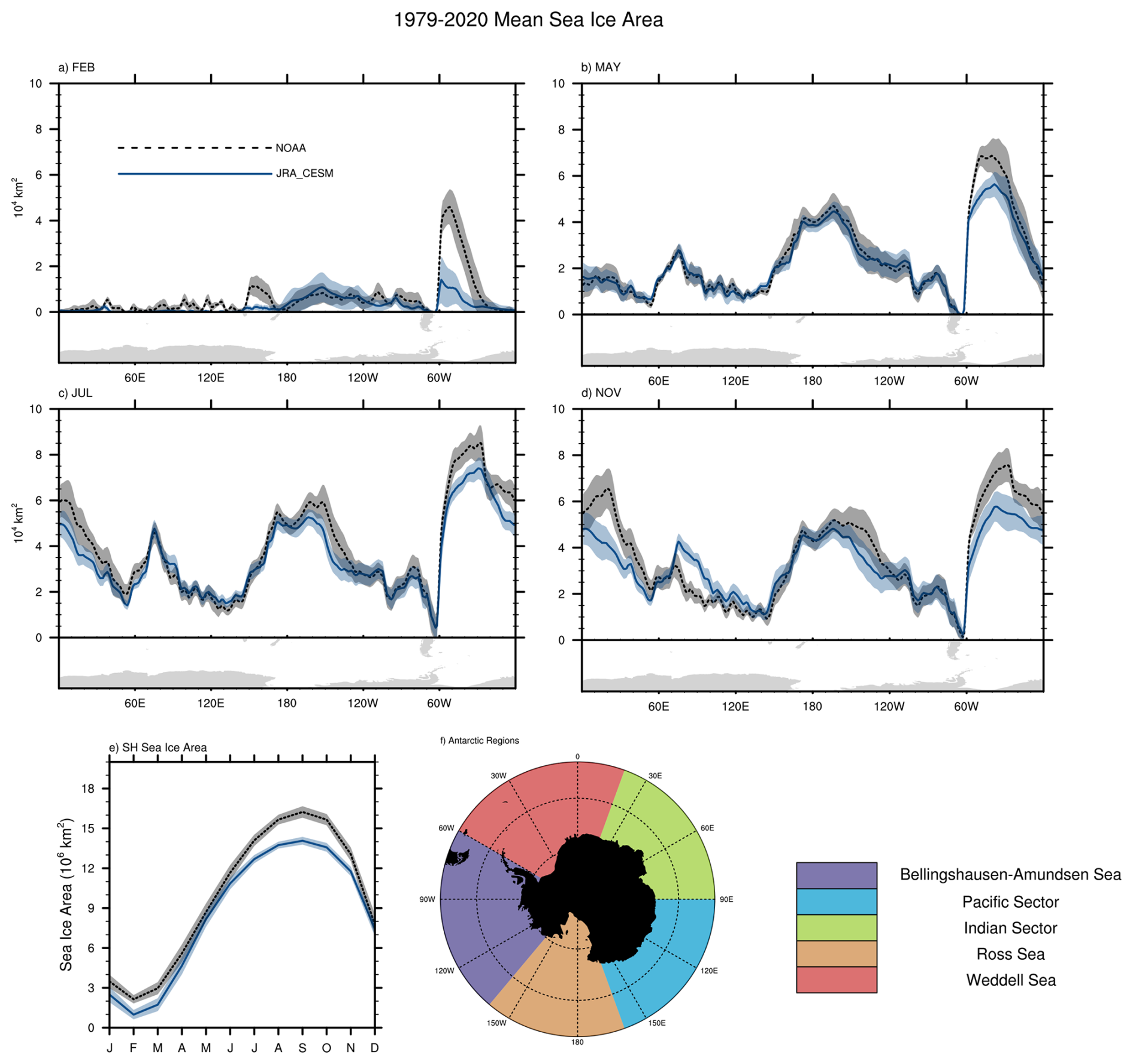
Figure 1 1979–2020 Monthly mean total sea ice area as a function of longitude for (a) February, (b) May, (c) July, (d) November, (e) monthly Southern Hemisphere (SH) sea ice area climatology for the NOAA CDR (black) and JRA-CESM (blue); and (f) Antarctic regions map. Thick dashed (NOAA) and solid (JRA-CESM) lines indicate the mean; shaded polygons indicate the mean ±1 standard deviation. Sea ice areas as a function of longitude have been smoothed by a 3-point running average.

4.2 Polynyas in the satellite data

Maps of open water and coastal polynyas on 15 July 2003, calculated using our algorithm and a SIC threshold of 85 % for observational datasets are shown in Fig. 2a–e. Note that this date is not special, but a representative day shown to illustrate differences in polynya identification metrics across products. We picked a random winter day as relatively few polynyas are identified in January–April in all data products, and the broad similarities and differences between polynyas identified in different data products on this winter day are typical.

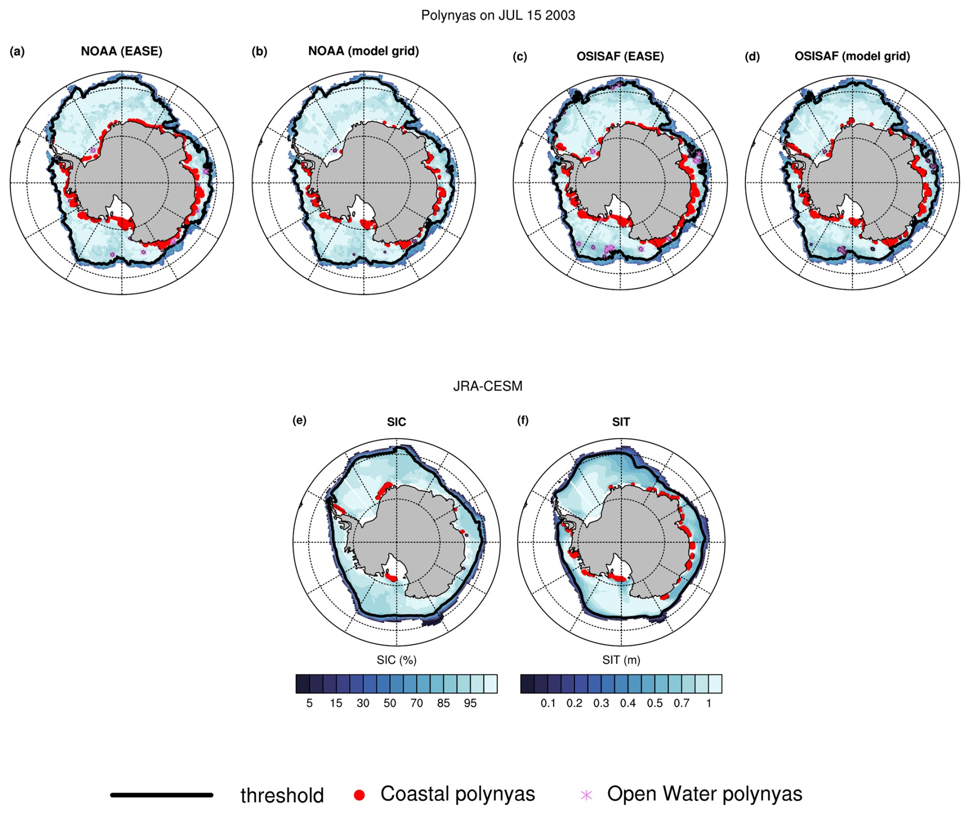
Figure 2 Polynya maps for 15 July 2003, using SIC 85 % threshold for the NOAA and OSISAF CDR data on the original Equal Area Scaleable Earth (EASE) grid (a, c), the NOAA and OSISAF data regridded to the CESM grid (b, d), the JRA-CESM (e) and the JRA-CESM using a 0.4 m SIT threshold (f). Open water and coastal polynyas are indicated by the pink stars and red dots. The 85 % SIC and 0.4 m contours are indicated by the thick black contours over the colour contoured SIC or SIT values. Sea ice concentrations below 15 % are masked out.

The sea ice edge (defined as the 15 % SIC contour) is nearly identical for both the NOAA and OSISAF satellite products on the original grid and after regridding to the nominal 1° climate model grid (Fig. 2a–d). More open water polynyas are identified in the OSISAF product than in the NOAA product. Differences in coastal polynyas identified in the two satellite products are more mixed, with more coastal polynyas identified on the east side of the Antarctic peninsula in the OSISAF CDR than in the NOAA CDR, regridded or not, yet more coastal polynyas are identified in the Weddell Sea in the NOAA product than in the OSISAF product on the EASE grid. Regridding has a greater impact on polynya areas in the NOAA product than on the OSISAF product (Figs. 2a–e and 3a–d). We show both open water and coastal polynyas identified in our example day, however we focus on coastal polynyas for the remainder of this study.

4.2.1 Southern Hemisphere polynya statistics in satellite based products

When moving beyond an example day and looking across all years, regridding the observational products from the original EASE grid to the model grid has a larger impact on both number and area of polynyas identified in the NOAA product than for the OSISAF product (Fig. 3a–d). The climatological winter and spring polynya areas and number of polynyas at a given SIC threshold in both observational products show only small changes when using monthly vs. daily data (after regridding to the model grid). Integrated Southern Hemisphere (SH) coastal polynya areas as well as number of polynyas are larger in the NOAA product when identified on the original finer-resolution EASE grid than when regridded to the 1° CESM grid in both winter and spring across the full range of SIC thresholds. Polynya areas in the regridded NOAA product are nearly the same using both daily and monthly averaged data. On the other hand, regridding the OSISAF data to the model grid leads to larger polynya areas and higher numbers of polynyas at SIC thresholds below ∼70 %, with smaller differences (within 1 standard deviation range of polynyas identified on the EASE grid at daily resolution) higher thresholds. Like in the NOAA data, the differences in the climatological polynya areas and numbers between regridded daily and monthly data are quite small (Fig. 3a–d; see Fig. S3 for summer, DJF, and fall, MAM). Although integrated SH polynya areas are nearly identical across a range of thresholds from both satellite products on the original EASE, daily grid, regridding has opposing impacts on polynya identification in the two satellite products. After regridding to the model grid, consistently higher polynya areas and numbers are identified in the OSISAF data than from the NOAA data for both seasons and across the entire range of thresholds. Variability in SH polynya areas tends to be larger during the spring, particularly at high SIC thresholds, and continue to increase into the summer as areas of low/thin sea ice within the icepack merge with surrounding open ocean as the sea ice melts and contracts (Fig. S3).

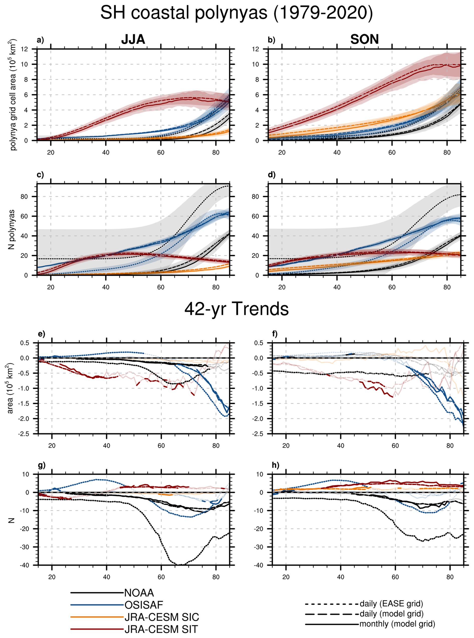
Figure 3 Total SH mean (1979–2020) coastal polynya areas (a–b), number of polynyas (c–d), 42-year trends in polynya areas (e–f) and 42-year trends in number of polynyas (g–h) as a function of threshold value (SIC, SIT) for winter (JJA; left column) and Spring (SON; right column) for NOAA (black), OSISAF (blue), and JRA-CESM (SIC metric, orange and SIT metric, maroon). x axis units are 15 %–85 % for SIC and 15–85 cm for SIT. Polynyas identified using the daily observational data on the original EASE grid are shown by dotted lines; dashed/solid lines indicate polynyas identified using daily/monthly data on the model grid. Climatological mean (1979–2020) values are shown in the thick lines; ±1 standard deviations shown by the lighter shading (a–d). Dark, thick dots/dashes/lines in the trend figures (e–h) indicate 95 % or higher significance based on the Mann-Kendall non-parametric trend significance (Mann, 1945; Kendall, 1975; Gilbert, 1987).

Trends in polynyas identified in the observational products differ by retrieval method, SIC threshold and spatial and temporal grids. Significant negative trends (and no significant positive trends) are seen for the NOAA daily CDR on the EASE grid in both seasons across all SIC thresholds for the number of polynyas, and at SIC thresholds less than ∼76 %/72 % for the JJA/SON integrated polynya areas. On the other hand, polynyas identified in the OSISAF product show significant positive trends in area (JJA) and number (JJA, SON) at low SIC thresholds, and significant negative trends at high SIC thresholds (SH polynya areas and numbers, both seasons). After regridding to the model grid, integrated SH polynya trends are negative and significant only in the winter and at SIC thresholds lower than ∼75 % in the NOAA product and significantly smaller in magnitude (up to ∼3-fold), and yet negative in both seasons in the OSISAF product and at SIC thresholds higher than ∼65 %. These inconsistencies in trends across thresholds, observational data products and grids are also apparent in the regionally integrated timeseries except for the Bellingshausen-Amundsen sea region which shows significant negative trends in polynya areas for both CDRs, on both the EASE and model grid, across a range of thresholds for the winter season (Figs. S4–S8).

To better illustrate and compare relationships between polynya areas, numbers and locations, we show in more detail polynyas identified in observational and model data at select SIC and SIT (model) thresholds. We pick threshold values such that the resultant seasonal coastal polynya areas and numbers are consistent with published work (e.g. Arrigo and van Dijken, 2003; Arrigo et al., 2015; Tamura et al., 2008; Nihashi and Ohshima, 2015), as outlined in our methods section, and such that integrated SH polynya areas are roughly equal in both seasons between all data sources and grids. We recognize that there is not one clear choice of metrics and therefore our thresholds are somewhat arbitrary. Alternative threshold choices we have tried do not change our results (not shown). The metrics and thresholds we use for the satellite products are SIC threshold values of 78 % for the EASE daily and 85 % for the regridded NOAA (daily and monthly) data, and 75 % for the OSISAF (all grids). Although in general the integrated SH polynya areas are very similar between these metric choices in these data products, there are some small differences in areas, numbers of polynyas, and variabilities (Figs. 3a–d, 4). Notably, a larger number of distinct polynyas are consistently identified in the OSISAF data than in the NOAA data (regridded to the 1° grid and monthly averaged), and thus even though the SH polynya areas are quite similar, the average polynya size in the OSISAF is smaller than in the NOAA product.

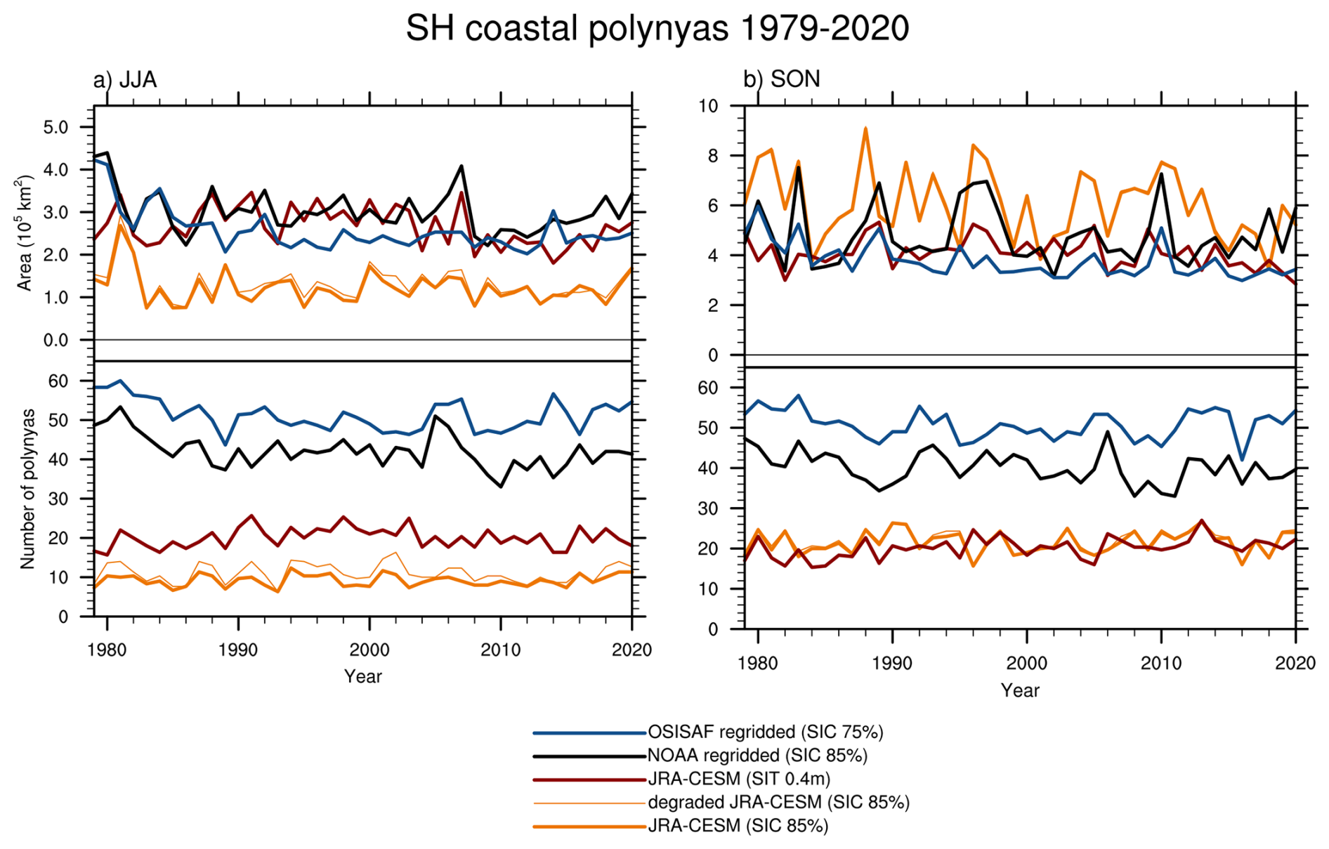
Figure 4 Southern Hemisphere (SH) 1979–2020 winter (JJA; a) and spring (SON; b) mean coastal polynya area (top panels) and number of individual polynyas (bottom panels). Polynya timeseries are for monthly NOAA (SIC 85 %; black) and OSISAF (SIC 75 %; blue) CDR data regridded onto the CESM grid, JRA-CESM model simulation using monthly SIC (85 %; orange) and SIT (0.4 m; brown), and the JRA-CESM model SIC degraded to more closely mimic satellite SICs (85 %; orange thin line).

Correlation coefficients reveal impacts of regridding (spatially and temporally) as well as relationships between the two observational products (Fig. 5). Regridding then monthly averaging the SICs before identifying polynyas results in a significant loss of self-correlation within the NOAA product, particularly for integrated SH polynya areas. Notably, timeseries of SH polynya areas from the daily data on the EASE grid and from the regridded, monthly averaged grid are not significantly self-correlated for either season for the NOAA data product. Cross-correlations for polynyas identified from the two observational products are significant only for polynyas identified from daily data (EASE and model grids), however the SH polynya timeseries (both areas and numbers) are not significantly cross-correlated between the observational products after regridding and monthly averaging. Self- and cross-correlations are comparable for the number of polynyas identified from the daily data (Fig. 5b). Additionally, the cross-correlation coefficients between the daily observational products, although significant, are ∼0.7 (area) to ∼0.75 (N), suggesting considerable variability in the time series due to the nuances of the retrieval algorithms.

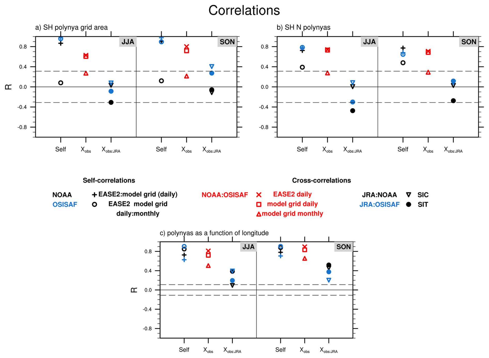
Figure 5 Correlation coefficients for integrated SH polynya areas (a), number of polynyas (b) and polynyas as a function of longitude (c) for each JJA (left) and SON (right). Self-correlations are calculated between different grids (“regridding”) for same observational product (NOAA black; OSISAF, blue); cross-correlations between the two observational products (NOAA:OSISAF, red) and between the observational products and the JRA-CESM (obs:JRA; NOAA black; OSISAF, blue). Symbols show correlations between time/longitude polynya time series from the daily observational data on the original EASE grid vs. daily (+) and monthly (o) regridded on the model grid; NOAA:OSISAF on the EASE grid (x) and then regridded daily (□) and monthly (open triangles); and between JRA-CESM polynyas identified using SIT 0.4 m (•) and SIC 85 % metric (inverted open triangles). Dashed horizontal lines in a-c indicate the 95 % significance level based on the Mann-Kendall non-parametric trends significance (Mann, 1945; Kendall, 1975; Gilbert, 1987).

4.2.2 Regional polynyas in the satellite data

Winter (JJA) and spring (SON) polynya areas as a function of longitude show both similarities as well as differences resulting from choice of CDR (NOAA vs. OSISAF), temporal (daily vs. monthly) and spatial grids (EASE vs. model; Fig. 6). Higher polynya areas are identified, for example, by the NOAA data in the Ross Sea region and near the Antarctic peninsula in the OSISAF product. In general, polynya areas identified using the regridded daily product are higher in both CDRs than those identified using the daily data on the EASE grid or the monthly regridded data.

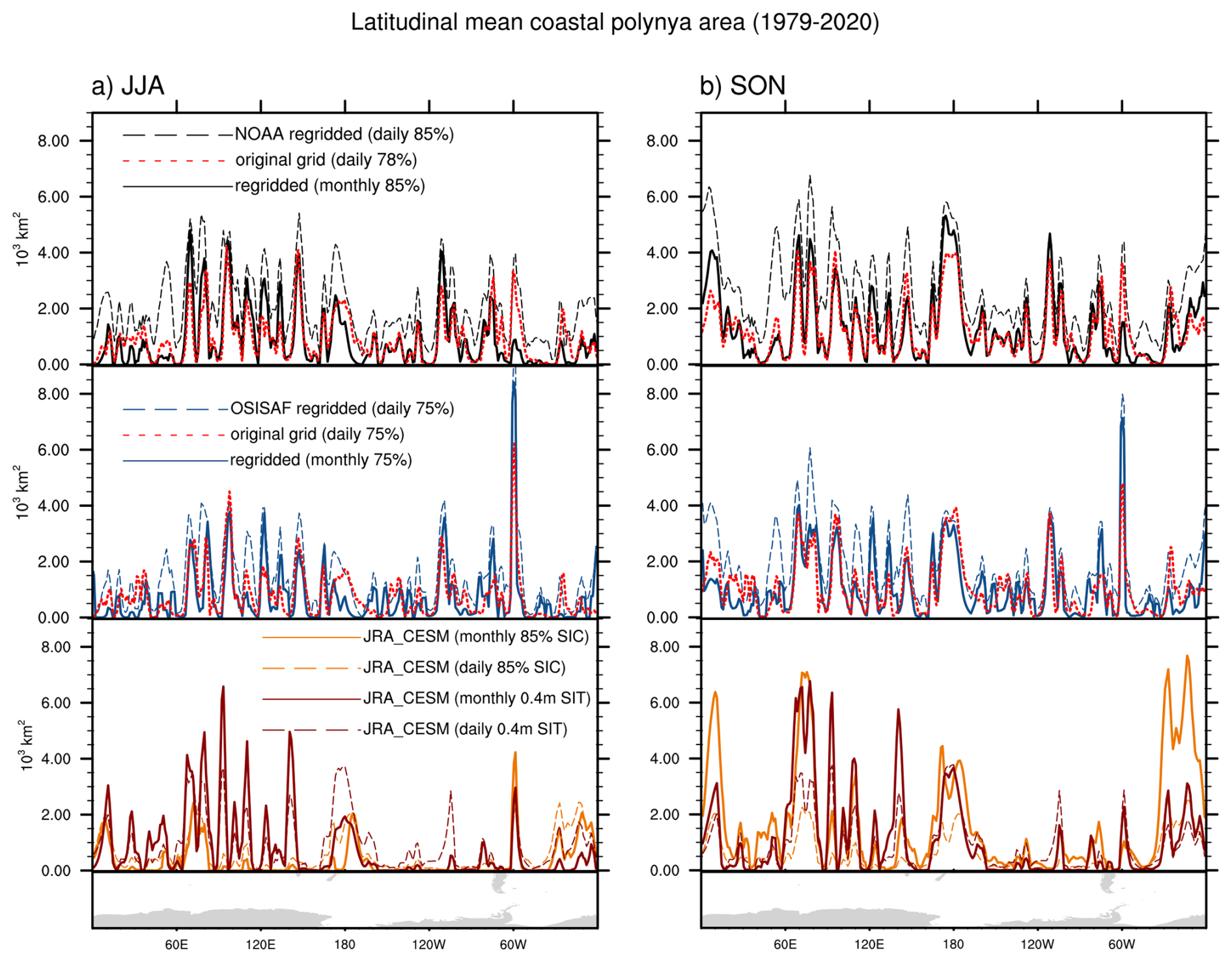
Figure 6 Winter (JJA; a) and summer (SON; b) mean coastal polynya area as a function of longitude for the NOAA CDR (top), OSISAF CDR (middle) and JRA-CESM (bottom). Polynya area as a function of longitude is shown as a 3° (longitudinal) running average. Top and middle panels show polynya areas for the three different grids and metrics – daily NOAA (78 % SIC) and OSISAF (75 % SIC) on the original grid (red dotted lines), CDR daily data regridded onto the CESM grid (NOAA 85 % SIC black and OSISAF 75 % blue) dashed lines, and regridded and monthly averaged (NOAA 85 % SIC, black and OSISAF 75 %, blue) solid lines. Bottom panels in (a) and (b) show polynya areas based on JRA-CESM model simulation using different polynya thresholds: monthly (solid lines) and daily (dashed lines) SIC at 85 % threshold (orange) and monthly SIT at 0.4 m (brown) thresholds.

Regridding and monthly averaging SICs from the CDRs has lower impact on spatial self- and cross-correlations than on the SH integrated temporal correlations (Fig. 5c). Climatological, coastal polynya areas as a function of longitude from the OBS data products show significant self- and cross-correlations regardless of temporal resolution or spatial grid and are generally higher than the temporal correlations. Unlike the temporal self-correlations, the longitudinal self-correlations are higher for polynyas identified on the monthly-averaged regridded data than for the daily regridded data.

Cross-correlations on regionally integrated timeseries are significantly correlated between the two observational data sources after regridding and monthly averaging only in the winter season in the Bellingshausen-Amundsen sea and the Indian sector (R∼0.4–0.5, respectively; Fig. S9). In all other regions and in these regions in the spring, polynya areas and numbers estimated from the regridded and monthly averaged observational data products are not significantly cross-correlated (Fig. S9). Self-correlations tend to be higher for polynya areas rather than polynya numbers, and the NOAA self-correlations after regridding and monthly averaging (original EASE grid, daily: model grid monthly) are insignificant for all seasons and regions, except winter in the Bellingshausen-Amundsen sea.

Regional trends in polynya areas, when significant, are generally negative for both seasons with the exception of the Pacific sector, which has only significant positive trends at high SIC thresholds for both seasons, and in the Indian sector where significant trends are generally positive in both NOAA and OSISAF for SIC thresholds below ∼80 % (JJA) or 55 % (SON), and significantly negative in the OSISAF at SIC thresholds above ∼80 % (JJA)/73 % (SON; Figs. S4–S8).

4.3 Polynyas in the JRA-CESM vs. NOAA and OSISAF OBS

4.3.1 Integrated Southern Hemisphere polynya area

Polynya-like features have been found in CESM2 (DuVivier et al., 2021; Singh et al., 2020), and the CESM2 reproduces many characteristics of Antarctic sea ice quite well, making it a suitable model for closer investigation of polynya-like features. Polynyas identified in the model and the observations may disagree if the model doesn't adequately capture mechanisms for producing polynyas, or due to model bias, or both. It is also possible that identification of polynyas in model output may require different metric choices than those used to identify polynyas in satellite products due to differences in model vs. satellite data as outlined above.

Polynya maps for the example day, 15 July 2003, show how the 85 % SIC threshold identifies far fewer polynyas in the JRA-CESM than either the NOAA or the OSISAF CDRs (Fig. 2), suggesting that SIC may not identify polynya-like features in model output in the winter season. Indeed, monthly climatological (1979–2020) wintertime (JJA) SH polynya areas remain very small in the JRA-CESM across the full range of SIC thresholds (Fig. 3; summer and fall are shown in Fig. S3). During winter freeze up, open water can freeze very quickly in the model, resulting in high SICs and yet relatively thin SITs. Monthly climatologies of SH polynya area reveal that SIT thresholds, unlike SIC thresholds, identify large areas of wintertime coastal polynyas across a range of SIT thresholds (Fig. 3). Both integrated SH polynya areas and numbers are nearly the same regardless of whether they are identified in the model output using daily or monthly data.

To compare with polynyas identified in the observational products, we use polynyas identified in the JRA-CESM using thresholds of 85 % SIC and 0.4 m SIT (and we show results in Figs. S10–S11 using a SIC threshold of 50 % SIC and SIT of 0.2 m for comparison). Figure 4 shows time series of SH polynya area and total number of SH polynyas for winter and summer, and underscores many of the complications comparing polynyas estimated from satellite products to those estimated using climate model output on a seasonal basis. There are significant seasonal differences in polynyas identified using these two metrics: polynya areas identified using the SIT metric are roughly three times as large as those identified using the SIC metric (and much closer to the SH polynya areas in both OSISAF and NOAA CDRs) for winter (JJA), whereas the magnitude of SH polynya area is similar using these thresholds in the spring (SON; Fig. 4). Fewer discrete polynyas are identified in the JRA-CESM using both SIT and SIC metrics than in either observational product in both seasons, even though the polynya areas are similar and thus the average polynya size will be smaller in the observations than in the model.

Temporal cross-correlations for SH polynya area, 1979–2020, between the NOAA, OSISAF and JRA-CESM are significant only between the OSISAF and the JRA-CESM using the SIC metric in the spring (SON; Fig. 5) – although it is interesting to note that the cross-correlations between regridded, monthly NOAA and OSISAF polynya area or number time series are not significantly correlated in either season. Trends (1979–2020) in SH polynya area in the JRA-CESM are significant and negative only for the polynyas identified by the SIT metric, and for a limited range of thresholds in both winter and spring (Fig. 3).

4.3.2 Regional polynya areas

Integrated mean SH polynya areas are very similar between the observational and model data for the metrics used, yet there are subtle regional differences. For example, climatological integrated SH polynya areas show very little difference whether using daily or monthly data (e.g. Fig. 3), and yet the longitudinal maps reveal that the daily SIT data identify more wintertime polynyas than the monthly SIT data in the Ross and Bellingshausen-Amundsen seas (Fig. 6). Wintertime polynyas in the Bellingshausen-Amundsen sea are particularly anaemic using the 85 % SIC metric (daily and monthly). In contrast, in spring (SON) the SIC threshold identifies higher modelled polynya areas in this region and they are closer to the polynya areas identified in the NOAA and OSISAF. Like the cross-correlations between the polynyas in the observational products, spatial cross-correlations between polynyas in the model and the observations are higher than temporal ones. Spatial cross-correlations between polynya area as a function of longitude identified in the satellite products and the JRA-CESM polynya area significant and positive for both metrics (SIT, SIC) and both observational products (NOAA, OSISAF) in the spring (SON), and SIT (NOAA, OSISAF) and SIC (OSISAF) in the winter (JJA; Fig. 5).

Regional trends are generally not significant in the model for most SIT and SIC thresholds (Figs. S4–S8), although there are some regionally significant trends for the SIT (0.4) metric, both negative (SIT: Ross, JJA; Weddell JJA and SON) and positive (SIT: Bellingshausen-Amundsen Sea, SON) as well as significant negative trends in wintertime Indian sector polynyas identified using the SIC metric.

4.4 Impacts of different definitions for sea ice concentrations in the model and satellite data

Discrepancies between polynyas identified using SIC in the model and the observational data may arise due to differences in SIC definitions in satellite-based versus model data, particularly during the winter months. As discussed above, sea ice can form immediately in the model during the cold austral expansion season and through the winter, thus resulting in SICs that are high even though the ice may be very thin. Satellite imagery cannot differentiate between water and sea ice at very low SICs or low sea ice thicknesses. To understand potential impacts that these model and observational differences in SICs may have in polynya identification metrics, we degrade the model SIC output to more closely mimic satellite estimates of SIC. In areas of low (<10 % SIC) or thin (<5 cm SIT) ice, we set daily SICs to 0 % SIC, and in thin ice areas (5–20 cm SIT) the originally modelled SICs are reduced by half. We then identify polynyas using an 85 % SIC threshold on the degraded model output.

Comparisons of the standard model to degraded output indicate that degrading SICs results in small, positive differences that are largest within the ice pack during ice growth season and along the ice edge in the winter (Fig. 4 and Appendix C); differences from degraded output during the sea ice retreat season (SON) are much smaller with no discernible patterns (not shown). Degrading the model data results in lower SICs throughout much of the fall pack ice and along the winter sea ice edge, and these differences show very little regional variability and do not consistently explain the model bias of the non-degraded data compared with the satellite products and in some cases would further increase model-observational biases. Identifying polynyas based on the degraded model data (using an 85 % SIC threshold) results in an increase in wintertime polynyas by ∼10 %–20 % (Figs. 4 and S12–S13). This increase is quite small compared to the model (using the SIC threshold) versus CDR polynya area differences. Thus, it does not explain the differences in polynya areas estimated from these three products and we focus on results using the standard model output (non-degraded) for the remainder of this paper.

4.5 Relationships between polynyas and NPP in the JRA-CESM

Net primary productivity (NPP) describes the rate of photosynthetically fixed carbon in the upper ocean; it quantifies the energy available for marine food webs. In the high-latitude Southern Ocean, NPP increases markedly as the sea ice retreats and light returns to Antarctic waters (e.g. Richert et al., 2019, and references therein). Light reaches the surface sooner in polynyas than the surrounding ice-covered areas, relieving phytoplankton of light limitation (e.g. Arrigo and van Dijken, 2003). We look at polynya regions defined in the austral spring (SON), to see if the model captures high NPPs within identified polynyas during the early growth season as is found in observations. The choice of metric (concentration or thickness) to identify SON polynyas in the model is not clear based on the previous analysis that indicates not only differences between the two observational products with respect to polynya areas, temporal and spatial correlations and trends, but also that polynyas identified in the JRA-CESM using a 0.4 m SIT and 0.85 % SIC thresholds each have seasons and/or regions that better correlate with the NOAA or with the OSISAF. We therefore use austral spring polynya regions as identified by both the 0.4 SIT and the 85 % SIC metrics for the NPP analysis.

Comparing the monthly average NPP per unit area within austral springtime coastal polynyas and within the sea ice zone allows us to better understand how polynyas may augment austral spring NPP and thus play a critical role in the Antarctic food web (Fig. 7). Note that the SIZ, which is defined as the area covered seasonally with sea ice (as determined by the 1979–2020 mean winter – JJA – 85 % SIC contour) covers significantly more ocean area than the spatial area of polynyas, so the net production within the SIZ is larger than in polynyas (Fig. 7, top). However, we find that the NPP per unit area is substantially higher during the austral spring in regions identified as polynyas using both SIC and SIT polynya identification methods than it is within the SIZ in general (Fig. 7, bottom). This finding suggests that the model does indeed capture high productivity within low and/or thinner ice regions. Additionally, the higher NPP per unit area persists into the summer and early spring (December–March) as well. Polynyas have a particularly large impact on NPP during December, when area average NPP within polynyas is more than twice as much as within the SIZ when using the 0.4 m SIT threshold and 1.5× higher when using the 85 % SIC threshold. Although the total integrated SON polynya area is an order of magnitude smaller than the total SIZ area, NPP within polynyas contributes ∼17 %–23 % of the total NPP during the December peak. These results highlight that polynya-like features are playing an important role in Antarctic marine productivity in the CESM2.

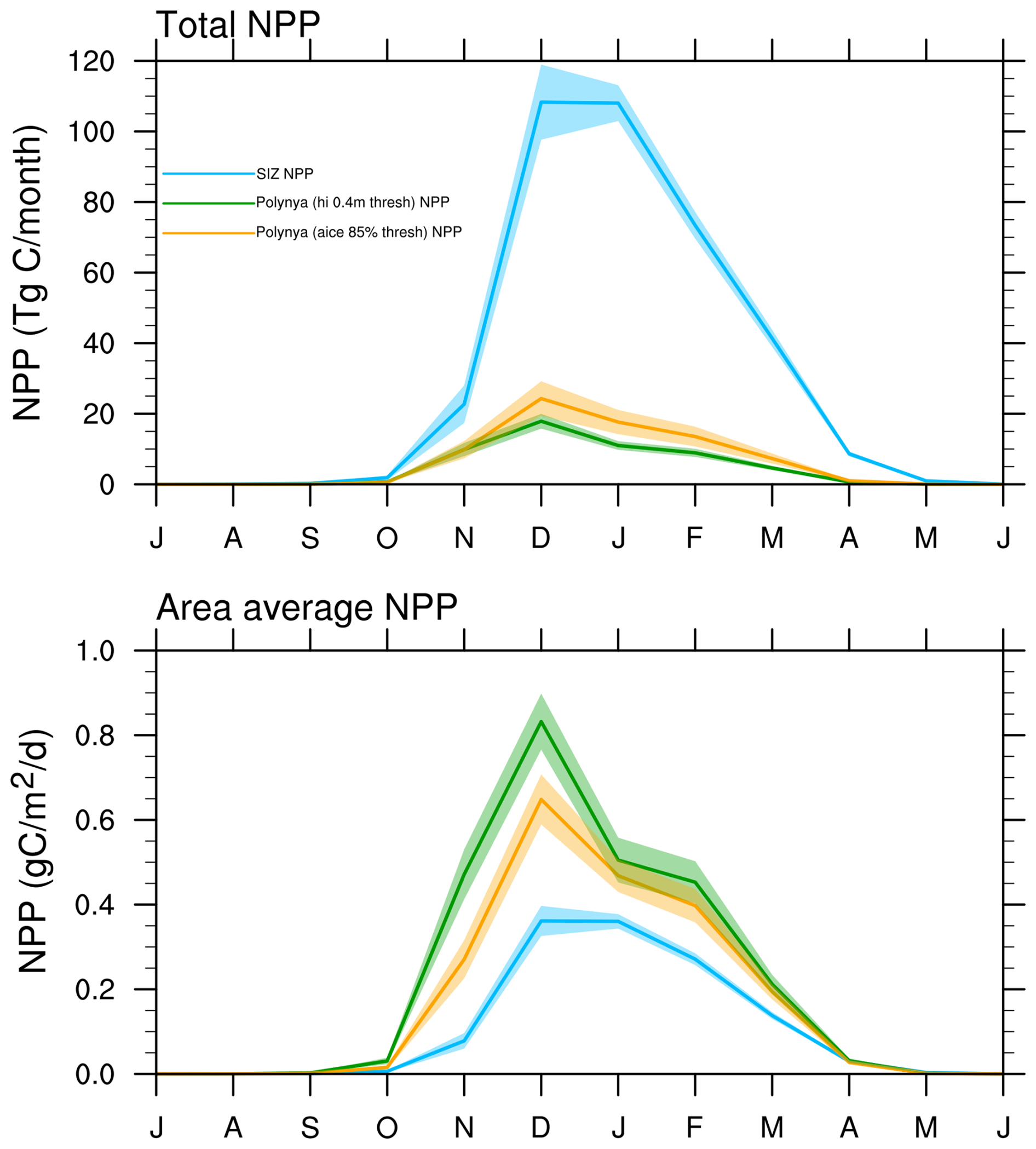
Figure 7 JRA-CESM 1979–2020 climatological integrated SH monthly total NPP (top) and area-averaged NPP (bottom) for the sea ice zone (SIZ: blue) and SON polynya regions identified using 0.4 SIT (green) and 85 % SIC (orange) thresholds.

5 Discussion

Polynyas are often qualitatively defined – “open water surrounded by ice and/or ice and land” – and a leading conclusion of this work is that care must be taken when identifying quantitative polynya data from gridded products. Polynyas are a feature of the sea icescape – a complex, dynamically changing structure that is an integrated component of polar marine ecosystems as well as a leading player in polar oceanic and atmospheric circulations and dynamics.

Ideal metrics and thresholds for polynya identification will depend on the product grid sizes, region of interest, season and scientific application, as well as the specifications of an individual data product. Many coastal polynyas occur on smaller scales than can be resolved by the original EASE grids of the satellite based SIC products much less the typical nominal 1° grid of ESMs. An important result of this work is that although grid size may preclude resolving many individual polynyas (particularly many coastal polynyas), “polynya-like features” may indeed be identified.

Gridded SICs retrieved from satellite images reveal much about the sea icescape, yet different retrieval algorithms can result in extremely small differences in hemispheric and regional integrated sea ice extents and areas, and simultaneously significant differences in temporal variability, correlations and trends in sub-grid scale features, as shown in this analysis of polynyas identified using SIC thresholds. These differences may be partially due to the difficulty of capturing areas of low SICs and/or low SITs through remote sensing, although disentangling the sources of these discrepancies is beyond the scope of this work.

That the same passive microwave data but different retrieval algorithms can lead to uncorrelated timeseries of SH polynya areas and numbers once the data have been regridded and averaged monthly is remarkable. Polynya areas identified in both observational products are, however, significantly correlated spatially (longitudinally), regardless of spatial (EASE vs. model) and temporal grids (daily vs. monthly). This result suggests that on a climatological scale, locations of polynya-like features identified in both observation products are consistent even if their temporal variability, correlations and trends are not. Spatial cross-correlations between polynya features identified in the JRA-CESM output are significant, albeit lower than between the two observational products. The CESM2, like many ESMs, does not simulate land fast ice and therefore landfast ice cannot serve as anchors for coastal polynyas in the model which may contribute to this discrepancy.

Inconsistencies between identified polynyas in these two observational products complicate comparisons with ESM output, which are typically on coarser grids and daily or monthly averages rather than daily snapshots. Polynya features identified within both observational products and the JRA-CESM are consistent in terms of climatological means and geographic locations, even as temporal correlations, variabilities and trends are inconsistent between all the products (when on the same grid). The highest spatial (longitudinal) cross-correlations between the JRA-CESM and NOAA polynyas are nearly as large as cross-correlations between the two observational products (after regridding). The JRA-CESM successfully simulates polynya-like features in the icescape along the Antarctic coast, in a manner that is spatially consistent with both the NOAA and the OSISAF products, although the JRA-CESM tends to simulate lower polynya areas in the Bellingshausen-Amundsen sea than those estimated from the either product. Polynya-like features identified in the JRA-CESM show significantly higher NPP in these features identified using both SIT and SIC thresholds, than in the sea ice zone as a whole, and thus this method of identifying polynya-like regions successfully identifies biological hotspots in the model: NPP within polynyas in the JRA-CESM contributes to about 18 % of the total Antarctic SH marine NPP even though the sea ice zone is roughly ten times as large as the springtime coastal polynya areas.

We provide some “best practices” from this systematic comparison of polynya identification methods in satellite-based and the CESM below and discuss the implications of polynya metric choices for applications in climate models.

5.1 Polynya metric choices: Temporal and spatial resolutions

Analysis of polynyas identified in both satellite and model products suggest that integrated SH climatologies made from daily vs. monthly data do not differ significantly, and thus monthly data may be sufficient for some analyses on longer temporal scales. Integrated polynya (area and number) timeseries self- and cross-correlations are reduced when regridding the observational SIC data, to the point that regridded (from EASE to model grids) monthly data from the two observational products are not significantly correlated – yet the spatial cross-correlations remain significant even after regridding between the two products. Thus, the method used here identifies polynya-like features that are geographically consistent between the two regridded observational products and yet inconsistent in temporal variability. We therefore recommend that in order to eliminate discrepancies due to grid types and resolutions alone, we recommend comparing metrics from data on the same grids (temporal and spatial), and regridding – if necessary – data with the higher geographical resolution onto the coarser resolution grid. Trends in polynya areas are not robust – including in significance, magnitude and sign – across the range of SIC thresholds, grids and product sources (retrieval algorithms) in the observations analysed here. These inconsistencies between temporal variabilities, cross-correlations, and trends, and consistencies in geographical cross-correlations between polynyas in the two observational products suggest that the observational products may serve as good (poor) sources of verification of polynyas in ESM data spatially (temporally).

5.2 Polynya product and metric choice in modelled data

Using SICs, in general, to identify SH wintertime coastal polynyas in model simulations requires very high thresholds and is particularly problematic in the Bellingshausen-Amundsen Sea. Part of this issue is likely because ocean surface waters can very rapidly refreeze and form very high sea ice concentrations in all models, not just the CESM. Degrading model output to more closely resemble satellite estimates of SICs leads to only small increases in polynya areas identified using SICs (at 85 % threshold) and does not explain the large bias between polynyas identified in winter (JJA) in both observational products and the JRA-CESM. We thus find that identification of wintertime polynyas in the CESM better reproduces observed polynyas when using a SIT-based threshold, which more accurately accounts for low sea ice areas than SICs, which can be very high in the model even in very thin sea ice conditions, unlike in satellite imagery. We anticipate that other models will also have large discrepancies in wintertime coastal polynyas identified using SIT vs. SIC and suggest considering a SIT-based metric for winter-time coastal polynya identification from model output.

It is interesting to note that while significant longitudinal correlations exist between polynya features identified in the JRA-CESM and the OBS for each month of the year and annually (Fig. 4c), the same cannot be said for temporal correlations of the integrated time series (Figs. 5c and 6a–e). This suggests that the regionality of the identified polynyas in the JRA-CESM is captured well compared to the observations, however the temporal variability is less well captured in some regions and seasons. Part of this may be explained by the reanalysis data used to force the JRA-CESM and the nature of coastal polynyas. Reanalysis wind products show the lowest biases compared with weather station data in regions and times of high synoptic and/or low katabatic wind activity, and significant biases in wind fields close to the coast near where katabatic winds significantly impact coastal winds (e.g. Jones et al., 2016; Caton Harrison et al., 2022). Katabatic winds are integral to the formation of coastal polynyas (e.g. Thompson et al., 2020, and references therein). Thus, coastal polynya variability due to variability in katabatic winds may be captured by the polynya time series in the observations but not well represented in the atmospheric reanalysis data used to force the model.

Recent work found significant positive trends in annual polynya areas in the Ross, Weddell, Indian and Pacific sectors estimated using daily data from the OSISAF CDR product at a 50 % threshold on the 25 km × 25 km EASE grid (Duffy et al., 2024). Our results show significant positive polynya area trends in the OSISAF on the EASE grid only in the Indian sector (JJA and SON) and integrated across the SH (JJA) with a 50 % SIC threshold. These contradictions may be due to differences in metrics or methods used to identify polynyas – an analysis beyond the scope of this work – yet it highlights that caution should be taken when comparing results from different sources, grids, methods and metrics. Indeed, one of our primary conclusions from this work is that trends of polynya-like features identified on grids that may not truly resolve distinct polynyas (as opposed to polynya-like features) should be viewed with caution, as different thresholds may result in even different signs of significant trends.

5.3 Polynya applications: coastal polynyas and NPP in a changing climate

Our analysis with the JRA-CESM demonstrates that the CESM is indeed capturing enhanced productivity within polynya-like features in austral spring compared to within the entire SIZ. Elevated rates of NPP occur in polynya features identified using either a 0.4 m SIT or an 85 % SIC thresholds, with similar rates of productivity in SIC and SIT-defined polynyas. NPP within these polynya-like features contributes ∼17 %–23 % of the total sea ice zone NPP during the December peak, even though the area of these polynyas is only ∼3 % of the sea ice zone. This finding underscores how critical polynyas are for the base of the Antarctic food web, and using models to understand these areas is particularly critical given the challenges of satellite chlorophyll retrievals in these areas (e.g. Oliver et al., 2025).

6 Conclusions

The definition of “polynyas” in a quantifiable sense is relatively subjective. Defining areas and timing of open water within the Antarctic sea ice zone such that comparisons can be made between satellite based SICs and model output requires careful consideration and recognition of the basic differences between satellite observations and model output as well as considerations of grid size, metric and threshold. Coastal polynyas exist often at spatial scales smaller than the grid scales from both observational and simulated data. As such, polynya metrics may not resolve polynyas per se, but rather grid cells that contain polynya-like features. One of the most surprising results of this work is the astonishing inconsistencies between polynya area time series variabilities and trends due that result using different retrieval algorithms and/or regridding. Temporal trends show particularly large inconsistences – including in sign – across algorithm, grid, and threshold. These inconsistencies in temporal variabilities and trends of sub-grid scale icescape features such as polynyas suggest that temporal characteristics such as variability and trends may not be adequately captured by this method of identifying polynya-like features on gridded data, whether in observationally based products or model output. On the other hand, polynya-like features are consistent spatially across both observationally based products and the hindcast model output.

Our conclusions with respect to our primary four questions are:

1. The JRA-CESM captures climatologically and biologically relevant coastal polynya-like features and coastal winter polynyas identified using sea ice thicknesses in model data are more consistent with wintertime polynyas identified in satellite-based products.

2. Temporal variabilities and trends are inconsistent not only between polynya-like features in the model and the observational products, but also between the two observational products, grid and threshold.

3. Spatial locations of winter–spring coastal polynya-like features are consistent between both NOAA and OSISAF, as well as between the JRA-CESM and both observational products.

4. Coastal polynya-like features in the JRA-CESM serve as biological hotspots, contributing ∼17 %–23 % of the total sea ice zone marine net primary productivity even while occupying only about 3 % of the area of the sea ice zone, consistent with observational studies.

Appendix A: Polynya algorithm

The polynya algorithm cycles through maps of the sea ice variable (concentration or thickness in this work) and initially labels any grid cells that fall below the threshold and that lie within the sea ice zone (south of the open ocean boundary). The algorithm iteratively cycles through the polynya maps to determine if grid cells that meet the threshold criteria are surrounded by sea ice and land (in which case they are labelled a polynya) or lie next to open ocean (in which case they are not identified as a polynya). Figure A1 shows a schematic of a hypothetical region with land, ocean, sea ice and polynya grid cells. In this example, there are two polynyas – one open water polynya (occupied by three grid cells), and one coastal polynya (occupied by two grid cells). Figure A2 shows an example satellite image of the Ross Bay and Terra Nova polynyas and grid cells labelled by SICs.

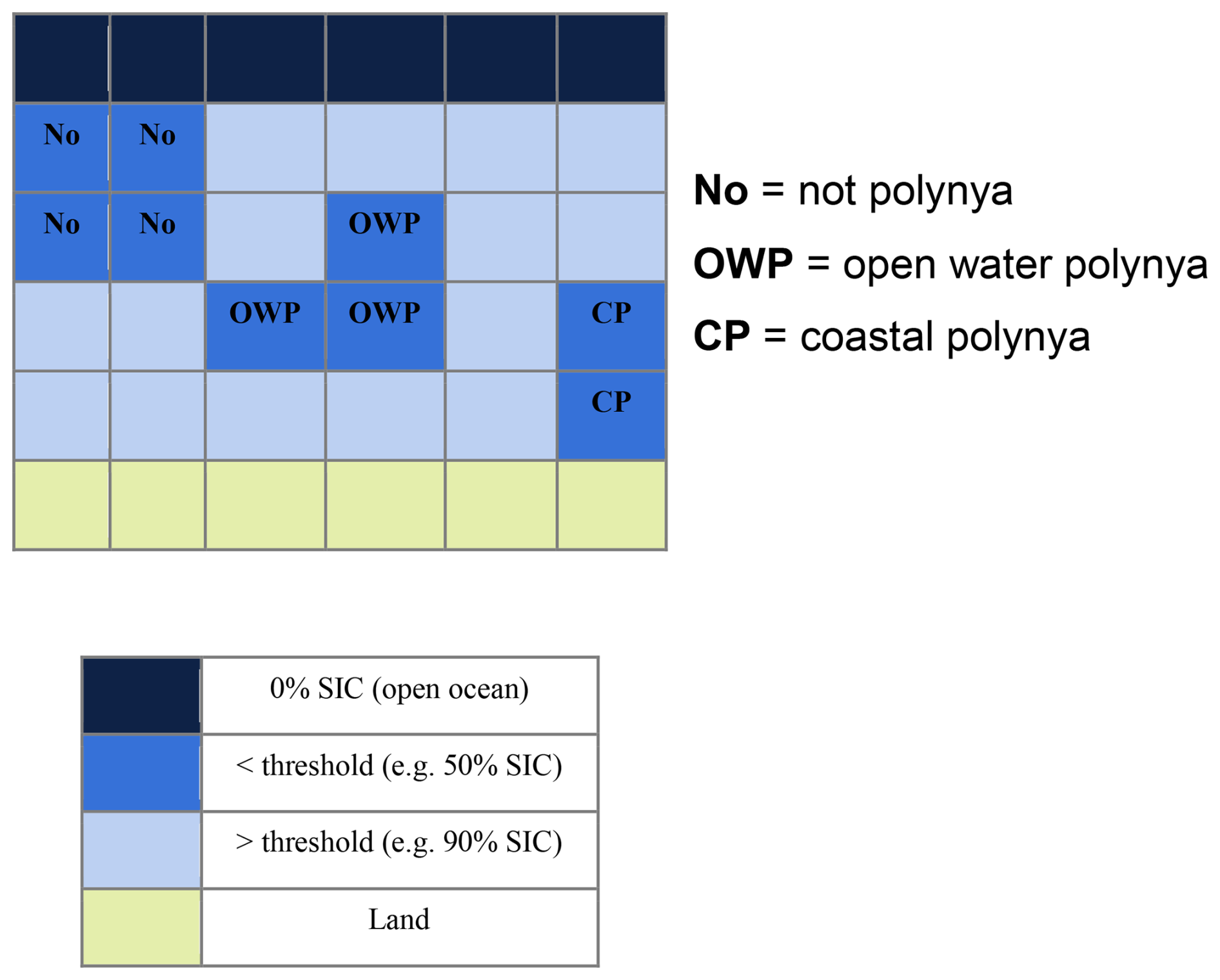
Figure A1 Schematic of grid cells considered open ocean (dark blue), land (light green) and within the sea ice zone (light and medium blue). Grid cells in the sea ice zone that meet the threshold criteria are in medium blue; grid cells that lie above the threshold are in light blue. Grid cells that meet the criteria are identified as polynyas only if they are bounded by sea ice (open water polynyas) or sea ice and land (coastal polynyas).

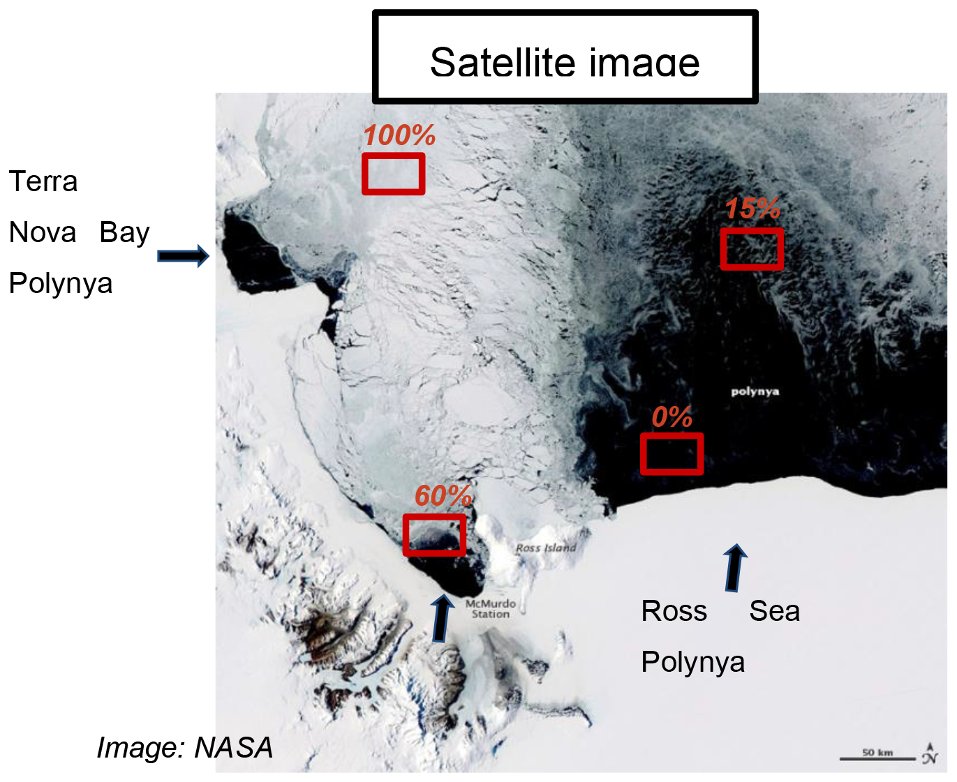
Figure A2 Example satellite image of the Terra Nova Bay and Ross Sea polynyas (Moderate Resolution Imaging Spectroradiometer (MODIS) image of the day from the National Aeronautics and Space Administration (NASA) Aqua satellite, 16 November 2011 https://eoimages.gsfc.nasa.gov/images/imagerecords/76000/76474/rosssea_amo_2011320_lrg.jpg, last access: 21 November 2011). Hypothetical grid cells with SICs are shown in red.

Appendix B: Grid size and type and impact on polynya identification

Using concentration thresholds to define polynya regions will define how much open water (and likewise sea ice) is in the grid cell by percentage. For an Equal Area Scaleable Earth (EASE) grid this will correspond to an area that doesn't change with latitude or longitude, whereas on an equal latitude-longitude grid a SIC percent threshold will correspond to different areas of open water (or sea ice) depending on latitude. For example, a 50 % sea ice concentration threshold on a 25 km × 25 km EASE grid corresponds to 312.5 km² or more of open water (and also 312.5 km² of sea ice) within the grid cell to meet the threshold requirement for a polynya. A grid based on latitude and longitude, which is common for earth system models, will have a varying range of surface area in each grid cell. A grid cell of $\sim \mathrm{3.2}\times {\mathrm{10}}^{\mathrm{3}}$ km² (about the area of grid cells next to the Antarctic coast on the Pacific and Indian sectors in the CESM) would have 312.5 km² of open water at a SIC threshold of 90 %. Figure B1 shows the area of the grid cells in the ocean grid in the CESM2 and areas of open water that would be contained in grid cells for example SIC thresholds. An example of the SIC thresholds required to result in 312.5 km² of open water within a grid are shown in Fig. B2 for an equal area grid cell and two grid cells from a 1° × 1° grid cell at two different latitudes. Different grids can also lead to different areas and numbers of polynyas even when the open water areas are the same (e.g. Fig. B3).

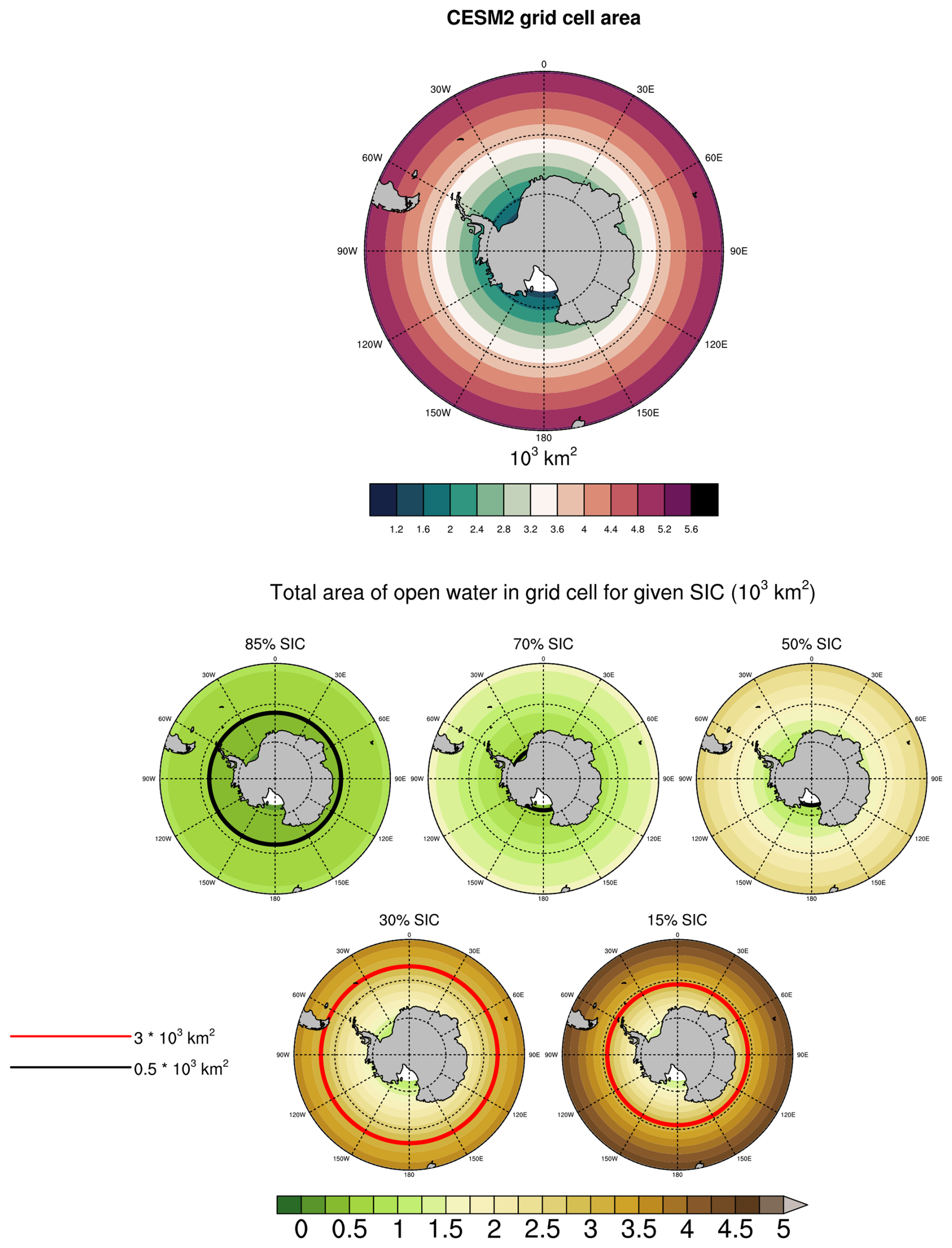
Figure B1 Area of the ocean grid cells in the CESM2 (×10³ km²; top) and total area (×10³ km²) of open water for a given SIC threshold in the CESM2 grid (bottom). Red/black contours indicate 3×10³ km²/0.5×10³ km² of open water, respectively.

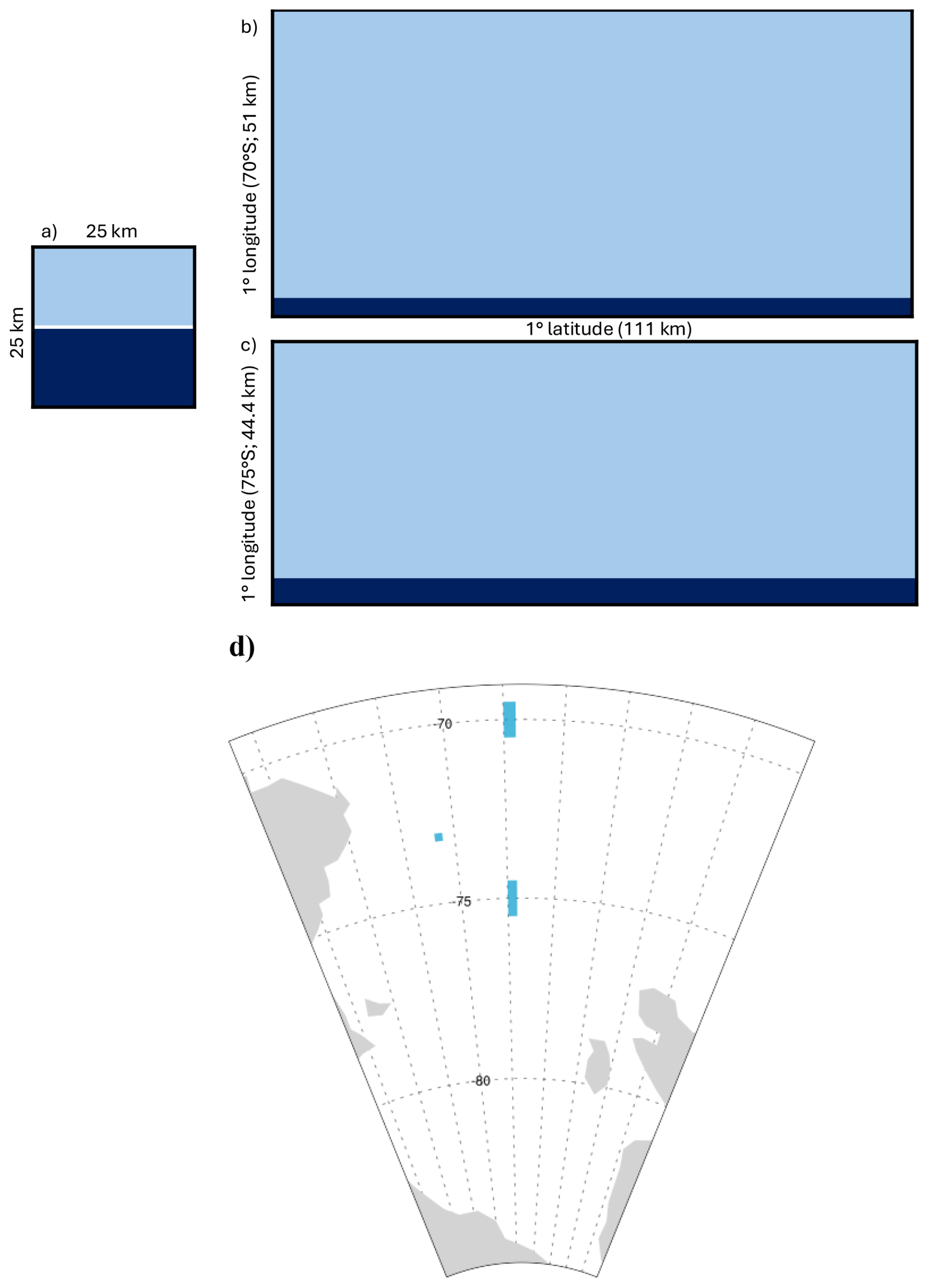
Figure B2 Sea ice concentration required to result in 312.5 km² of open water within a grid cell: (a) SIC 50 % on a 25 km × 25 km equal area grid cell, (b) 94.8 % SIC on a 1° × 1° lat/lon grid cell at 70° S (approximately 111 km × 51 km), and (c) 93.7 % SIC on a 1° × 1° lat/lon grid cell at 75° S (approximately 111 km × 44.4 km). Panel (d) shows the area occupied by grid cells (in blue) in (a), (b), (c) in the Ross Sea as an illustration. Panels (a)–(c) are shown as rectangles for illustration even though 1° lat/lon grid cells are not exactly rectangular.

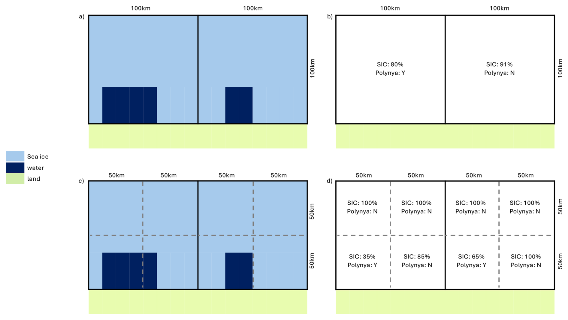
Figure B3 Examples of grid cells classified as polynyas using an 80 % SIC threshold on a larger resolution grid (a–b) and a smaller resolution grid (c–d). Coloured panels (a, c) indicate areas of ice (light blue), water (navy) and land (light green). Text in panels (b), (d) indicate SIC for the grid cell and whether or not it would be identified as a polynya using an 80 % SIC threshold. The top example has one polynya grid cell and double the integrated polynya area (10 000 km²) over the entire region compared to the second example (2 grid cells and 5000 km²).

Appendix C: Degrading climate model daily SIC data

Figure C1 shows an example of model SICs that are degraded such that the new sea ice concentrations are set to 0 where the original SICs are less than 10 % and where SITs are less than 5 cm. In regions of SITs that fall between 5 and 20 cm, SICs are set to half of the original values. The resulting degraded product has noticeably lower SICs along the ice perimeter and isolated locations near the Antarctic continent with lower SICs.

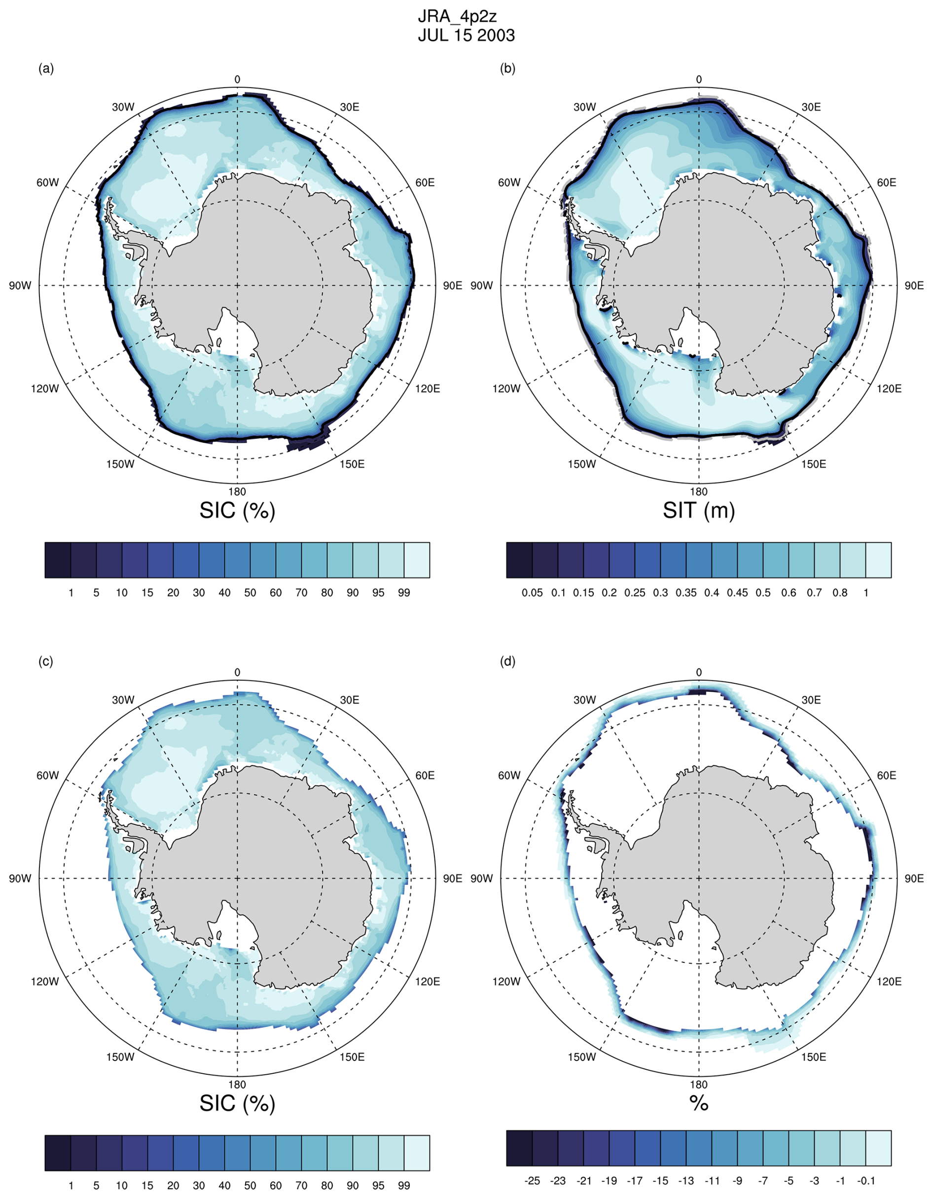
Figure C1 Sea Ice Concentration (a) and sea ice thickness (b) from the JRA-CESM run on 15 July 2003. Degraded sea ice (c, d) the resulting change in SIC by degrading the sea ice.