Beyond MAGT: learning more from permafrost thermal monitoring data with additional metrics

Metrics such as the mean annual ground temperature (MAGT) and active layer thickness (ALT) are used to monitor and quantify permafrost change. However, these have limitations including those arising from the effects of latent heat, which reduce their sensitivity. We investigated the behaviour of existing and novel metrics derived from temperature observations (TSP metrics) using an ensemble of more than seventy 120-year simulations. We evaluated which TSP metrics provide new insight into permafrost change and evaluated how reliably each one indicates changes in sensible, latent, and total heat contents for different levels of sensor quality. We also quantified the effect of sensor placement on the magnitude of observed MAGT trends.

We observed depth-related differences in decadal MAGT warming rates of more than 0.23 °C decade⁻¹ (50th percentile) for observation depths between 10 and 20 m. The magnitude of these differences is reduced to 0.17 °C decade⁻¹ (50th percentile) when considering the thermal integral($\stackrel{\mathrm{‾}}{\mathit{\tau }}$) – A metric describing a depth-averaged warming trend. The effect of sensor depth on warming trends is greatest in ice-poor soils.

In warm permafrost, we find that depth of zero annual amplitude (d_za) and mean annual surface temperature (MAGST) exhibit qualitatively different behaviour than MAGT which can help disambiguate low or imperceptible warming rates by the latter metric. Finally, we recommend a parsimonious set of five TSP metrics to provide a better picture of permafrost thaw than MAGT or ALT alone. These are: height of the permafrost table (TOP), d_za, $\stackrel{\mathrm{‾}}{\mathit{\tau }}$, mean annual ground temperature (MAGT), and MAGST.

Our results can be used to inform permafrost monitoring strategies and help contextualize observed trends. Consistent metrics can be produced from observed and simulated thermal data via the ”tspmetrics” library available on the Python Package Index (PyPi).

1 Introduction

Permafrost is an important component of the global climate system (IPCC, 2022) and its changes affect ecosystems, infrastructure, and ways of life in high-latitude (Meredith et al., 2019) and mountainous (Hock et al., 2019) regions. Ground temperature is the most common variable in permafrost monitoring and one of three products used to characterize the permafrost Essential Climate Variable by the World Meteorological Organization (Sessa and Dolman, 2008; Smith and Brown, 2009). Temperatures are usually recorded at discrete depths in boreholes with thermistor chains and data loggers. The way in which the resulting T(z,t) data, i.e., temperature at different depths (z) and times (t), are processed into summary metrics determines what conclusions can be drawn during interpretation and what value can be derived from the investment in thermal monitoring. We argue that current practices for processing and reporting permafrost thermal monitoring data overlook important information and can be improved by including additional metrics.

To conceptualize the utility of differing metrics, common uses of ground temperature monitoring data can be grouped by the relevance of changes in three key quantities: (1) sensible heat content (H_s), which directly reflects temperature changes. (2) Latent heat content (H_l), which reflects the melting or formation of ground ice; and (3) total heat content (H_t), which is relevant for subsurface heat storage (Cuesta-Valero et al., 2023; von Schuckmann et al., 2023).

Most often, long-term changes in permafrost are described using mean annual ground temperature (MAGT) measured near the depth of zero annual amplitude (d_za) where the annual temperature amplitude is dampened to less than 0.1 °C (e.g., Romanovsky et al., 2010). These observations typically use temperature measurements from a single sensor 10–25 m deep, where some of the temporal and spatial variability present at shallower depths is smoothed out. Inferring permafrost change using MAGT trends at single depths entails five major shortcomings:

1. Latent heat changes are hidden in temperature observations. We can see this where temperatures are shown flatlining just below 0 °C and figure captions suggest a counterintuitive and ambiguous interpretation: that such periods with barely visible change in fact indicate fast ice loss in the ground (cf. Smith et al., 2010; Groenke et al., 2023).

2. MAGT changes are inconsistent temporally and spatially as a result of differences in the partitioning of latent and sensible heat. Temporally, the same temperature change at the ground surface can cause a strong MAGT response in cold permafrost but after years of warming only cause minute MAGT change when the borehole is close to 0 °C. Spatially, a borehole in ground with little ice may be warming fast while a nearby borehole in ice-rich ground may warm only slowly. This inherent inconsistency of the MAGT confounds spatial and temporal comparison, even though such comparisons are common (e.g. Smith et al., 2022; Biskaborn et al., 2019). Moreover, the sampling of locations of observation boreholes is known to be biased towards sites that are accessible, likely to contain permafrost, of scientific or practical interest, or in ground materials amenable to drilling (e.g. Noetzli et al., 2021; Biskaborn et al., 2019; Subedi et al., 2020). Such bias will affect average warming rates in a region, further obscuring any meaning that can be derived from averages.

3. MAGT is inferred using observations from a single sensor. In current reporting of MAGT there is no standardized measurement depth (other than generally being at or near d_za) and the metric is sometimes compared across sites at different depths. Differences in the choice of observed depth may further affect the relative timing and magnitude of the MAGT trends from different locations, however the magnitude of depth-related effects has not been reported.

4. Relying on MAGT alone forgoes valuable information that is usually recorded at other depths. Although MAGT provides direct insight into the thermal state of the ground at a specific depth, it masks changes occurring elsewhere in the soil profile and offers limited information about the physical processes and hazards associated with permafrost thaw, which often occurs closer to the ground surface.

5. Deep boreholes are rare. Observation at or near d_za is useful as a single statistic, however, restricting ourselves to boreholes of 10 m or more neglects many sites. Metrics suitable for shallower boreholes are therefore desirable, especially when considering the paucity of published ground temperature data (Brown et al., 2024).

In summary, these five shortcomings mean that using MAGT as the sole indicator of permafrost change presents an interpretation challenge, as its magnitude is not consistently proportional to any single property of interest.

With the goal of informing decision-making and permafrost research (cf. Gruber et al., 2023), we aim to better use T(z,t) observations for revealing permafrost change by complementing MAGT. We denote TSP metrics as summary numbers representing the annual thermal state of permafrost that are derived from T(z,t) data.

The objectives of this study are to:

1. Review and develop TSP metrics, formalizing their calculation where necessary.

2. Quantify the effect of MAGT sensor depth on observed warming rates.

3. Evaluate how well TSP metrics reflect sensible, latent, and total heat gains in permafrost using simulated observations.

4. Recommend a parsimonious set of TSP metrics for future use.

5. Demonstrate the utility of the metrics recommended with example data from the GTN-P database.

2 TSP metrics

Many techniques exist to interpret permafrost change from ground temperature records. Some are formalized and quantitative (e.g., MAGT) while others involve a qualitative interpretation (e.g., the development of isothermal conditions). Although temperature is our sole input variable, we aim to gain additional insight into the effects of latent heat.

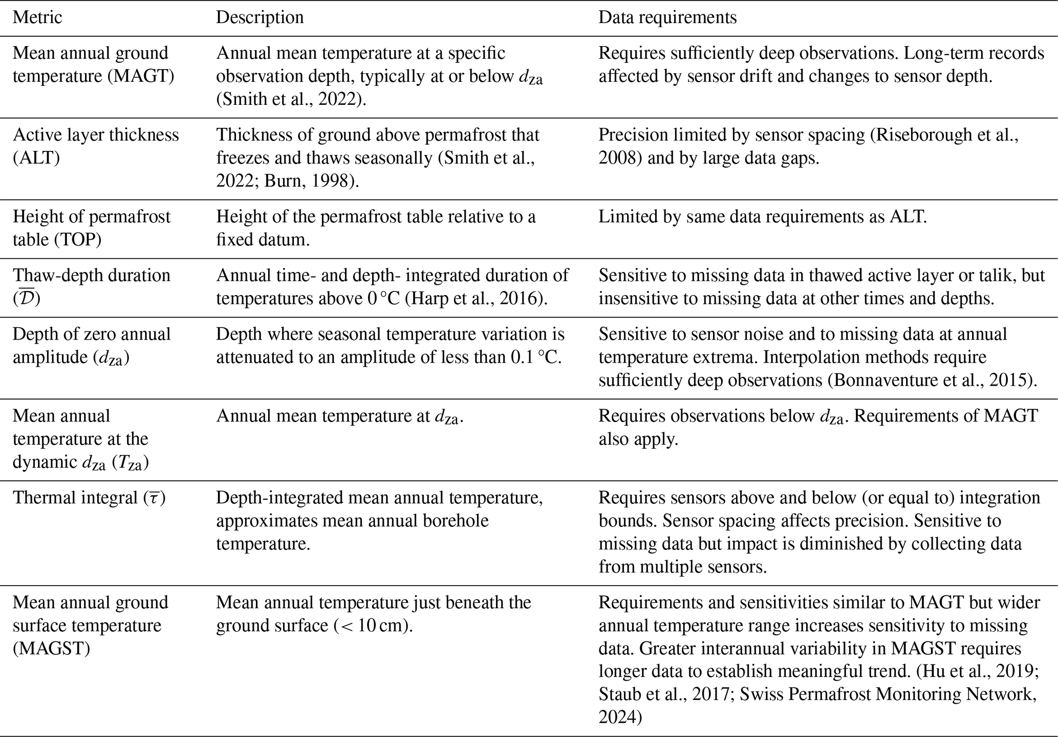
The metrics presented here (Table 1) produce annual summary values. They are derived from ground temperature observations reported for constant depths relative to the ground surface. In practice, ground subsidence may result in sensor depths that change over time. Most metrics are calculated from multiple sensors to represent an entire soil column and location. Only MAGT is based on a single sensor that must be selected. Where available, we also discuss observed rates of change for these metrics from existing monitoring efforts or other studies.

2.1 Mean Annual Ground Temperature (MAGT)

Measuring trends in MAGT is one of the most common ways to quantify permafrost change. The measurement of ground temperatures at or near d_za is established practice and effective at smoothing out inter-annual and fine-scale spatial variability. Typically, permafrost warming trends are calculated from sensors 10–25 m deep using linear regression of temperature time series (Isaksen et al., 2007; Smith et al., 2022) or Bayesian methods (Groenke et al., 2023).

We distinguish between MAGT measured at a specific fixed depth (denoted T_d at depth d) and mean annual ground temperature measured at the true d_za, the position of which is dynamic over time. We denote this latter metric T_za and discuss it below.

Observed rates of MAGT change are typically lower than 0.3 °C decade⁻¹ for warm permafrost ($>-$2 °C) and lower than 1 °C decade⁻¹ for cold permafrost ($<-$2 °C) (Smith et al., 2022). Biskaborn et al. (2019) estimated average warming rates as 0.39 °C decade⁻¹ in continuous permafrost, 0.20 °C decade⁻¹ in discontinuous permafrost, and 0.29 °C decade⁻¹ globally.

2.2 Mean Annual Ground Surface Temperature (MAGST)

MAGSTs provide information on changes to the upper boundary of a soil column, which propagate downwards to affect permafrost. Because they do not require costly drilling, MAGST measurements can be collected more economically than thermistor strings in boreholes, and enable denser data collection (e.g. Brown et al., 2022; Gruber et al., 2003). We calculate MAGST using model output at 0.1 m.

Systematic reporting of MAGST is less common than for MAGT or active layer thickness at permafrost research sites (Wang et al., 2024). In Switzerland, MAGST warming rates over permafrost have been estimated as 0.4–0.6 °C decade⁻¹ (1998–2022,  Swiss Permafrost Monitoring Network, 2024). On the Tibetan Plateau, MAGST warming rates were estimated as 0.16–0.60 °C decade⁻¹ (1980–2015, Hu et al., 2019) and 0.60 °C decade⁻¹ on average (1980–2007, Wu et al., 2012). Average trends across China (including non-permafrost regions) were reported as 0.20 ± 0.02 °C decade⁻¹ (1956–2022, Wang et al., 2024).

2.3 Active layer thickness (ALT)

ALT is one of three products used to monitor the permafrost Essential Climate Variable (Hu et al., 2025; Sessa and Dolman, 2008). Strictly speaking, its vertical extent is defined by the the greatest thaw penetration depth in a year, the maximum extent of the zero-degree isotherm is sometimes used as a thermal approximation of the active layer (Bonnaventure and Lamoureux, 2013). The thermally defined ALT has the advantage that it can be estimated using ground temperature records. This is often done by interpolating the two observations above and below the active layer (Streletskiy et al., 2017; Nelson and Hinkel, 2003). However, Riseborough (2008) found that the lowest error (equal to about 20 % of node spacing) was obtained by extrapolating from above using the two lowest sensors in the active layer, and by using instantaneous profiles rather than annual envelopes. The worst results were obtained when extrapolating from measurements below the active layer. Alternatively, some authors suggest fitting exponential curves to the ground temperature envelope (Nelson and Hinkel, 2003).

To estimate active layer thickness using the “extrapolation from above” method described by Riseborough (2008), we first calculate annual maximum temperatures at each sensor depth and identify the index (n) of the deepest sensor above permafrost where temperatures exceed 0 °C during the year.

Next, for each time step we determine the extrapolated thermal gradient using the deepest (z_n) and second-deepest (z_n−1) sensors above the isotherm

$$\begin{array}{}\text{(1)}& {\displaystyle \frac{\mathrm{d}T}{\mathrm{d}z}}\left(t\right)={\displaystyle \frac{T(z_n,t)-T(z_{n-\mathrm{1}},t)}{z_n-z_{n-\mathrm{1}}}}.\end{array}$$

The depth intercept of the zero-degree isotherm is then calculated as follows:

$$\begin{array}{}\text{(2)}& z_{T=\mathrm{0}}\left(t\right)=z_n+{\displaystyle \frac{\mathrm{0}-T(z_n,t)}{\frac{\mathrm{d}T}{\mathrm{d}z}\left(t\right)}}.\end{array}$$

Next, the process is repeated, but using the deepest sensor above permafrost with minimum temperature below 0 °C. This is repeated for all time steps in the year, and the active layer thickness is chosen as the greatest depth intercept. To estimate ALT by interpolation (ALT^↕), we use a similar approach, but calculate the thermal gradient using the nth and (n+1)^st sensors. Additionally, the position of the permafrost table can also be estimated by using only the maximum temperature in Eqs. (1) and (2). Finally, we average the two estimates of ALT. Long-term trends in ALT provide a minimum estimate for how much permafrost is lost due to thaw, but are insensitive to any additional ground lost due to thaw subsidence (O’Neill et al., 2023).

Observed ALT trends are typically low. Data from 109 active layer monitoring sites shows rates of increase generally between −0.2 to +0.4 m decade⁻¹ depending on the region, but up to +3.9 m decade⁻¹ in the Swiss Alps (Smith et al., 2022).

2.4 Height of the permafrost table (TOP)

In cold permafrost, our estimate of the ALT coincides with the depth to the permafrost table, or top of permafrost (TOP). However, if a supra-permafrost talik develops, this is no longer true. In that case, TOP continues to deepen independently of ALT causing the two metrics to differ by an amount equal to the talik thickness. Here, we neglect any differences between the thermal (cryotic) and physical (freeze-thaw) definitions of talik or active layer boundaries (Lewkowicz et al., 2025).

It is possible for TOP to change independently of ALT, so we consider TOP as an additional metric. To calculate TOP we use Eqs. (1) and (2) to estimate the position of the zero-degree isotherm.

2.5 Annual thaw-depth duration ($\stackrel{\mathrm{‾}}{D}$)

While change to ALT is commonly used as an indicator of thaw (Brown et al., 2000), it does not include any information about the duration of thaw. Both factors have implications for biological activity, terrain hazards, and carbon cycling. Harp et al. (2016) define ($\stackrel{\mathrm{‾}}{\mathcal{D}}$), a time- and depth-integrated value as

$$\begin{array}{}\text{(3)}& \stackrel{\mathrm{‾}}{\mathcal{D}}={\displaystyle \frac{\mathrm{1}}{\mathrm{365}}}\iint H\left(T\right(z,t\left)\right)\mathrm{d}z\mathrm{d}t,\end{array}$$

where T(z,t) describes the mean soil temperature at an arbitrary depth (m) and time (d) and H is the Heaviside step function. For each year, we select integration bounds from the ground surface to the top of permafrost, and from 0 to 365 d (simulations do not consider leap years). Practically, for daily observational data, we use a discretized form of this equation

$$\begin{array}{}\text{(4)}& \stackrel{\mathrm{‾}}{\mathcal{D}}={\displaystyle \frac{\mathrm{1}}{\mathrm{365}}}\sum _{j=\mathrm{1}}^{\mathrm{365}}\sum _{i=\mathrm{1}}^{N}H\left(\mathit{\tau }\right(z_i,t_j\left)\right)\mathrm{\Delta }z.\end{array}$$

Here τ is a linearly interpolated function of temperature with depth, discretized into N elements, and Δz is an arbitrary thickness increment, for which we use 0.01 m. Note that the use of interpolation rather than extrapolation across the zero-degree isotherm at the thaw depth may introduce a slight bias here (Hinkel, 1997).

2.6 Depth of Zero Annual Amplitude (d_za)

The depth at which the annual temperature amplitude is completely attenuated is denoted (d_za). A cutoff value of 0.1 °C in amplitude is typically used as a practical threshold.

Intuitively, we expect that d_za will be shallower for boreholes in which greater amounts of thaw take place, and in ice-rich boreholes where seasonal freezing and thawing decrease the apparent thermal diffusivity. This latter case indicates a greater potential for thaw. Over longer periods of time, increasing d_za should be expected to indicate a change to an increasingly latent heat-dominated system.

To estimate d_za we use the method described by Bonnaventure et al. (2015). Additional considerations for this calculation are described in Appendix E. First, the annual amplitude A_z at each observation depth, z, is calculated as half the difference between the annual minimum and maximum. Next, we fit coefficients x₀ and x₁ using least squares,

$$\begin{array}{}\text{(5)}& \ln \left({\displaystyle \frac{\mathit{A}}{A_{\mathrm{0}}}}\right)=x_{\mathrm{0}}-x_{\mathrm{1}}{\displaystyle \frac{\mathit{Z}}{Z_{\mathrm{0}}}}.\end{array}$$

where, A₀ and Z₀ are units of 1 °C and 1 m. For this step, we restrict the data by only using depth and amplitude pairs where A>0.5 °C so that temperature trends at depth do not add noise by inflating the amplitude. Finally, we calculate d_za using the fitted coefficients for each year of data

$$\begin{array}{}\text{(6)}& {\displaystyle \frac{d_{\mathrm{za}}}{Z_{\mathrm{0}}}}={\displaystyle \frac{x_{\mathrm{0}}-\ln \left(\mathrm{0.1}\right)}{x_{\mathrm{1}}}}.\end{array}$$

We are not aware of any long-term observations tracking d_za change over time. For the most part, d_za is treated as a static property to characterize or compare sites.

2.7 Dynamic Mean Annual Ground Temperature at the Depth of Zero Annual Amplitude (T_za)

Although MAGT is defined as the temperature at the depth of zero annual amplitude, it is typically recorded at a fixed depth below d_za in the range of 10 to 25 m.

We calculate a dynamic mean annual temperature at the depth of zero annual amplitude (T_za) whose position corresponds to the best estimate of d_za calculated above. After determining d_za, we interpolate the MAGT linearly to that depth to obtain T_za. Although this measurement technically describes a single depth, we consider it a borehole-aggregated metric because it is uniquely defined for any location, there are no choices to be made about its position, and it derives from more than one sensor.

As will be shown, T_za is the first ground temperature metric to become isothermal, and therefore can be used as a way to further classify borehole behaviour.

For clarity, we will use the acronym MAGT to refer to mean annual ground temperatures at a fixed-depth, and refer explicitly to T_za as necessary.

2.8 Annual Thermal Integral ($\stackrel{\mathrm{‾}}{\mathit{\tau }}$)

Monitoring ground temperature at a single depth provides a convenient summary statistic. However, it neglects data at other depths making it susceptible to sensor damage. Furthermore, the effect of unequal sensor depths between sites complicates meaningful comparison of warming rates between sites.

To investigate an alternative, we define the thermal integral ($\stackrel{\mathrm{‾}}{\mathit{\tau }}$) as the depth-integrated temperature evaluated between a near-surface sensor (z₁) and an arbitrary depth (z_n) of the mean annual temperature profile. This value is normalized by the integration depth, effectively yielding a mean column temperature.

$$\begin{array}{}\text{(7)}& {\stackrel{\mathrm{‾}}{\mathit{\tau }}}_{z_n}^{z_{\mathrm{1}}}={\displaystyle \frac{\mathrm{1}}{(z_n-z_{\mathrm{1}})}}\underset{z_{\mathrm{1}}}{\overset{z_n}{\int }}T\left(z\right)dz.\end{array}$$

Trends in the thermal integral correspond to mean column warming rates. Our hypothesis is that the trends will be more comparable between boreholes with unequal sensor spacing provided that the integration depths are similar.

Practically, to estimate $\stackrel{\mathrm{‾}}{\mathit{\tau }}$ from observations at discrete depths rather than from a smooth function T(z), we use the trapezoidal rule:

$$\begin{array}{}\text{(8)}& {\stackrel{\mathrm{‾}}{\mathit{\tau }}}_{z_n}^{z_{\mathrm{1}}}\approx {\displaystyle \frac{\mathrm{1}}{\mathrm{2}\left(z_n-z_{\mathrm{1}}\right)}}\sum _{i=\mathrm{1}}^{n-\mathrm{1}}\left(T\left(z_i\right)+T\left(z_{i+\mathrm{1}}\right)\right)\left(z_{i+\mathrm{1}}-z_i\right).\end{array}$$

where z_i is the depth of the i^th sensor.

(Smith et al., 2022)(Smith et al., 2022; Burn, 1998)(Riseborough et al., 2008)(Harp et al., 2016)(Bonnaventure et al., 2015)(Hu et al., 2019; Staub et al., 2017; Swiss Permafrost Monitoring Network, 2024)

Table 1 Summary of TSP metrics used in this study. Data requirements also include sensitivities to missing, biased, or inaccurate data.

3 Methods

3.1 Data pre-processing and conventions

Our processing uses daily T(z,t) data; sub-daily values are aggregated to daily averages first. For each annual period evaluated with TSP metrics, the number of daily values is reported and we exclude years with less than 95 % data completeness. We consider T(z,t) data to be reported for constant depths relative to the ground surface. In practice, ground subsidence may result in sensor depths changing over time. Multi-year trends in TSP metrics are calculated using ordinary least squares regression. For the model experiments, we calculate rolling trend windows of 5-, 10- and 20-year duration, representing data durations commonly available from permafrost monitoring today.

3.2 Quantifying the effect of depth on warming rates

We evaluate the effect of observation depth on MAGT trends and compare it to the effect of total integration depth on trends in $\stackrel{\mathrm{‾}}{\mathit{\tau }}$. For each trend window, the maximum difference in change rates of all depths between 10 and 20 m is calculated. For MAGT, this is done in two ways: first, by including all data, and again excluding any depths at which permafrost has degraded completely. Finally, empirical cumulative distribution functions are generated to quantify the effect of observation depth.

3.3 Ground temperature simulation

To simulate transient ground temperatures in a one-dimensional configuration, we use the model FreeThawXice1D – a numerical model of heat conduction with freezing and thawing in soils without water flow (Tubini and Gruber, 2025; Tubini et al., 2021). Energy conservation and model convergence is guaranteed at large time steps, making it suitable for ice-rich simulations requiring long spin up. Liquid water content, and thus freeze-thaw energy, is represented in the model using temperature-dependent soil freezing characteristic curves (SFCC). For our application we used the van Genuchten SFCC parametrization presented in Dall'Amico et al. (2011). FreeThawXice1D represents the effects of subsidence caused by ground-ice loss and accurately tracks 0 °C isotherms via local mesh refinement. Although advective water transport is not included in the governing equations, liquid water volume caused by excess ice melt and the associated latent heat is removed directly from the simulation.

We use GlobSim (Cao et al., 2019) to generate meteorological forcing data from the ERA5 reanalysis to drive the model at the upper boundary. This tool streamlines the download of reanalysis data, interpolates grid cells to point-scale to make data suitable for 1D simulation, standardizes units and time steps, and performs heuristic downscaling to account for terrain and other local effects. Future conditions are simulated by repeating several years of data with an added linear warming trend. More details on the simulation and the evaluation of resulting temperatures are presented in Appendix B.

3.4 Emulating imperfect observation data

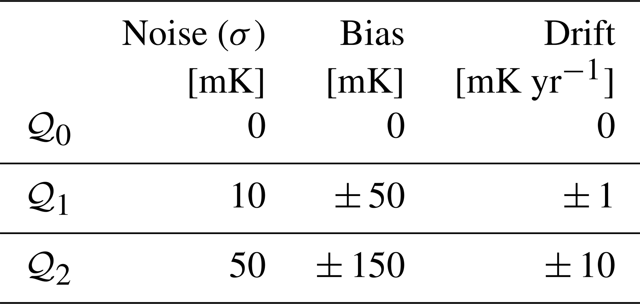
Simulation results are near-perfect data, with limitations related to model assumptions and numerical imprecision. To assess the sensitivity of TSP metrics to the quality limitations of real measurement systems, we degrade simulation results accounting for the accuracy (bias), drift, and precision (noise) of typical sensing systems (Appendix C). Based on typical performance characteristics, we create two additional data sets (Table 2) that emulate an excellent (𝒬₁) and a good (𝒬₂) commercial measurement system. The original model output is denoted (𝒬₀).

Table 2 The three levels of data quality: (𝒬₀) original simulation output, (𝒬₁) emulating an excellent monitoring system, and (𝒬₂) emulating a good monitoring system.

3.5 Evaluating TSP metrics as indicators of change

For each time window, TSP metrics are regressed against the change in heat content (sensible, latent, total). The strength of the relation – represented by the regression slope – is normalized by the standard error. The resulting values for the t-statistic, here analogous to a signal-to-noise ratio, are summarized in a histogram. Histograms are displayed to distinguish regression results by the statistical significance (p<0.05) and sign of the resulting trend.

The distribution of t-statistics across all trend windows is used as a measure of the reliability of a TSP metric as a way to detect heat-content changes in the ground. Positive slopes indicate true positives (sensitivity when expressed as a rate) and negative slopes indicate false positives (specificity when expressed as a rate). Spuriously significant regression can occur given the non-stationarity of our time series. Because all simulations are subject to similar levels of non-stationarity, the effects on relative efficacy of metrics is likely small.

3.6 Distinguishing stages of permafrost thaw

As will be shown below, T_za is the first mean temperature metric to reach isothermal behaviour near 0 °C. We investigate whether this metric can be used to partition the simulations into two distinct phases of thaw. For this particular experiment, we exclude bedrock simulations which have no appreciable ice content. For each simulation, we identify the breakpoint in slope (e.g., Fig. 1i) visually. Once the date is established, the mean trend in H_s and H_l are computed for the period before and after. Finally, the relative change in slope is computed as:

$$\begin{array}{}\text{(9)}& \text{Mean Trend Ratio}={\displaystyle \frac{m_{\mathrm{after}}}{m_{\mathrm{before}}}},\end{array}$$

where m is the corresponding mean trend. We also aim to develop a way to automatically determine the date of the breakpoint. For this, we use a quantitative threshold of four consecutive years of less than 0.1 °C of change in T_za. Finally, for comparison, we perform the same analysis using the commonly-used criterion to distinguish warm permafrost based on MAGT. That is, when MAGT of permafrost is between −2 and 0. We define the boundary as when T₂₀ reaches −2 °C for the first time; in our simulations this transition happens before the T_za breakpoint.

4 Testing TSP metrics with simulated data

We first interpret all simulations visually, in particular the behaviour in warm permafrost and redundancy between metrics. Then, we quantitatively compare how well the metrics represent changes in latent, sensible, and total heat content using regression.

In the experiment presented here, meteorological conditions are simulated for three different sets of spatial coordinates. These conditions are varied and extended using fixed offsets and warming trends, respectively (Appendix B). Simulations reflect a variety of surface and subsurface conditions: five different soil profiles are used, spanning conditions from water-free bedrock to fine-grained sediments with excess ice (Table B1). Combined with the different meteorological conditions, this resulted in 75 distinct simulations.

The output is produced with temperature and ice content up to a depth of 25 m (at 0.2, 0.4, 0.8, 1.2, 1.6, 2, 2.5, 3, 3.5, 4, 5, 7, 9, 10, 11, 13, 15, 20 and 25 m, cf. Harris et al., 2009) as well as for the elevation of the ground surface, total ice content, heat content (total, sensible, latent) of the soil column, and the positions of zero-degree isotherms.

4.1 Visual interpretation of example simulations

We present the results of two simulations as exemplars of the simulation ensemble and the behaviour of TSP metrics. The first simulation (Fig. 1a–f) is for a cold soil column containing no excess ice with an initial MAGT near −6 °C. Heat gain throughout the simulation is predominantly through sensible heat and approximately linear in time. All metrics exhibit a similarly linear response.

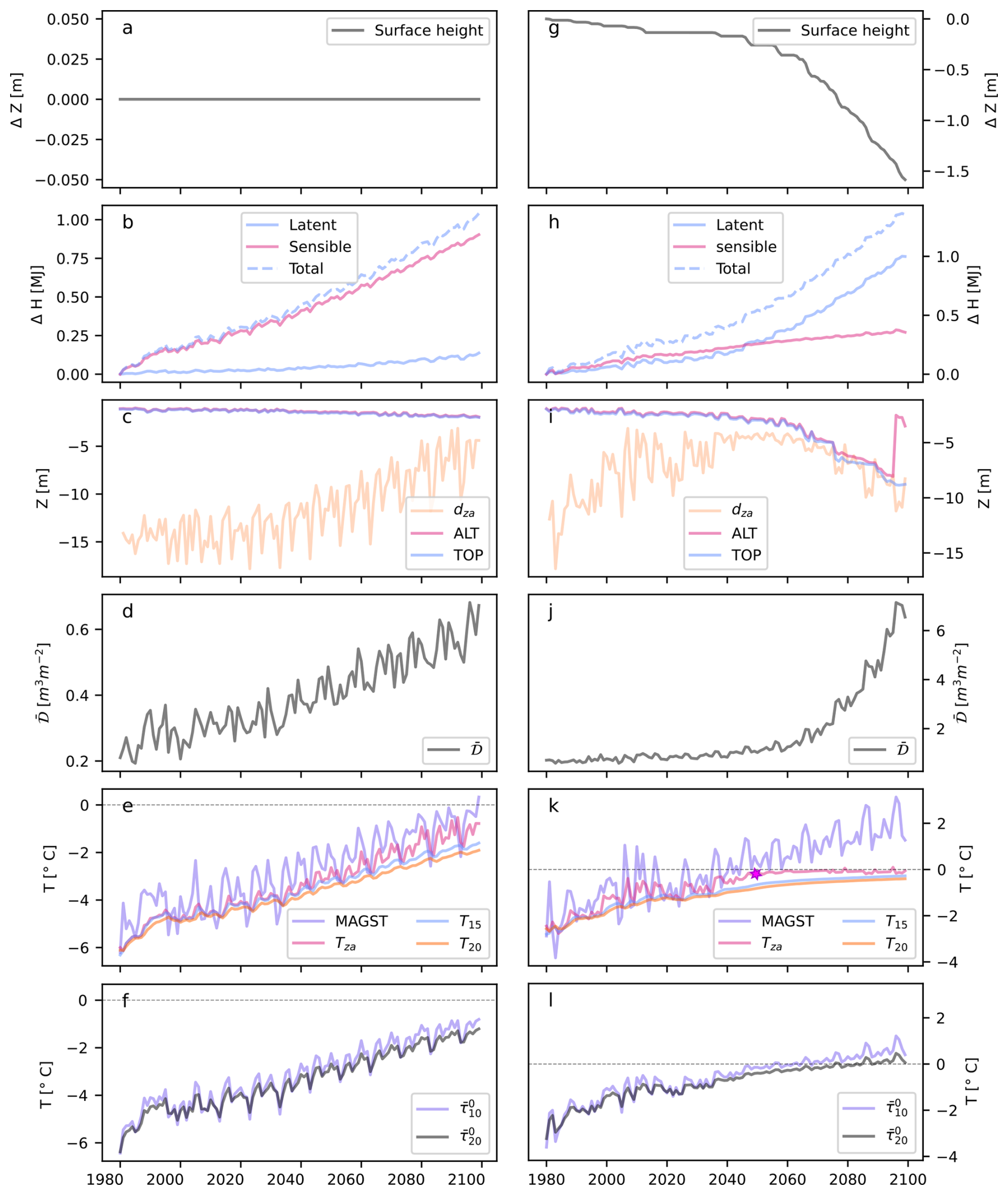
Figure 1 Warm and icy permafrost (g–l) exhibits much more nonlinear trends than cold permafrost (a–f) in metrics, surface height and heat content. Simulations allow us to visually compare different metrics. Here, we present 120 years of warming and the corresponding evolution of permafrost metrics for a cold simulation containing no excess ice (a–f) and for a warm simulation containing excess ice (g–l). Periodic variation from 2022 onward is due to the repetition of reanalysis data used to drive the simulation. In subplot (i), the purple star indicates the breakpoint in T_za when it becomes isothermal.

The second illustrative simulation (Fig. 1g–l) is for a column containing excess ice with an initial MAGT of around −3 °C. The loss of excess ice causes a decreasing ground surface height accompanied by an approximately linear increase in heat content. Unsurprisingly, the warming rate of MAGT is strongly dampened late in the simulation, demonstrating the challenge associated with interpreting this metric in the presence of latent heat transfer.

4.2 Permafrost thickness: ALT, TOP, and $\stackrel{\mathrm{‾}}{D}$

The ALT trend can be positive or negative in warm permafrost. When a talik develops, this causes a discontinuity in ALT followed by a reverse in the direction of the trend (Fig. 1i). This generally occurs in three stages: (1) An initial decoupling of ALT from the permafrost table when the ground no longer refreezes completely and a residual thaw layer persists. (2) A period when ground temperatures near 0 °C and multi-year temperature variability cause ALT to vary strongly, with occasional large jumps. (3) A more stable period (not shown in Fig. 1g–l) during which ALT decreases once the talik is well developed. ALT thinning has also been observed in the field (Connon et al., 2018).

In contrast to ALT, TOP declines monotonically during the warming period, indicating the loss of permafrost volume with less ambiguity as it is not reversing with the formation of a talik. Similarly, $\stackrel{\mathrm{‾}}{\mathcal{D}}$ is monotonic in its reaction to sustained warming. For the remaining analysis, we use TOP as the metric of choice, intuitively summarizing changes to the upper boundary of permafrost. Before the formation of a talik, changes in TOP, ALT, and $\stackrel{\mathrm{‾}}{\mathcal{D}}$ are very similar. This is not surprising given the considerable overlap between the definitions of these three metrics.

In warm simulations, we see that ALT, $\stackrel{\mathrm{‾}}{\mathcal{D}}$, and TOP change gradually for some time and then the rate of change begins to increase dramatically. This regime change between cold and warm permafrost has been previously described (Changwei et al., 2015; Wu and Zhang, 2010).

4.3 MAGT and T_za

Visually, MAGT behaves most similarly to borehole sensible heat content until it nears 0 °C, when warming rates decline in simulations with ground ice. Trends in T_za are similar to those of MAGT. However, in warming simulations with ice, T_za is the first depth to become near-isothermal because d_za becomes shallower as phase change takes place and temperature fluctuations are damped by latent heat transfer. The magnitudes of simulated trends in T_za and MAGT are similar.

In cold or moisture-poor permafrost, MAGT and T_za both generally follow a similar pattern as H_s. It is the effect of latent heat near 0 °C that dampens the warming trend in other cases. Because T_za is the first metric to reach isothermal behaviour, it is a good candidate for an additional metric. T_za also does not involve an arbitrary choice of depth but is derived from the behaviour of all observations. Otherwise, observations at a fixed depth, as commonly used for MAGT, are preferable to T_za because they are simpler to produce and understand.

4.4 Distinguishing stages of thaw

When simulations are partitioned into warm (MAGT $\ge -\mathrm{2}\mathit{°}C$) and cold (MAGT $<-\mathrm{2}\mathit{°}C$) permafrost, the mean H_l trend is significantly greater in warm permafrost than in cold permafrost (Fig. 2). This is not true of the H_s trend, for which the 95 % confidence interval of the mean trend ratio includes 1. On the other hand, when using a visually picked breakpoint in T_za (e.g., Fig. 1i) to distinguish two stages of thaw, we see that H_l trends are significantly greater in the later stages of thaw and H_s are significantly reduced. This is also true when the T_za breakpoint is estimated quantitatively rather than visually.

Another advantage of the T_za classification is that, because no specific depth must be chosen, the classification is valid for the entire borehole. Since d_za moves towards the surface, it also more likely that when the transition from one stage to another takes place, the sensors will be placed deep enough to measure this.

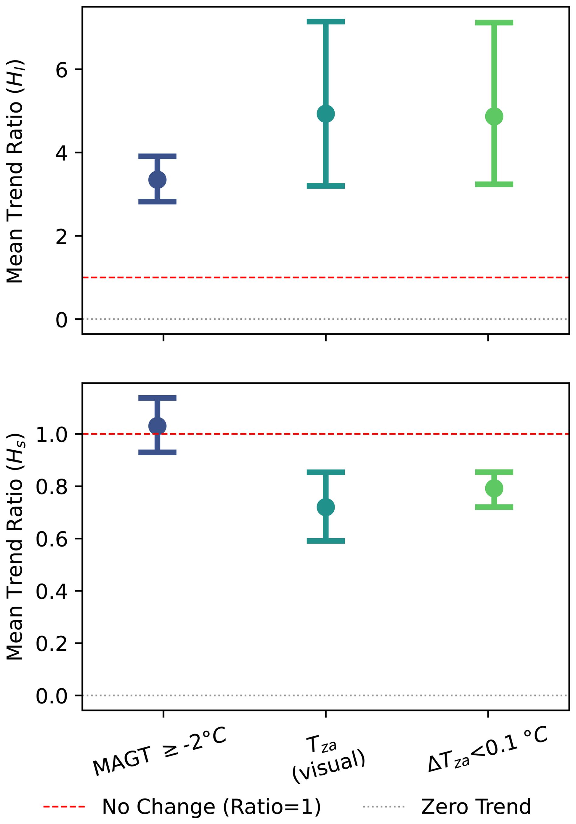
Figure 2 The distinction between warm and cold permafrost (MAGT $\ge -\mathrm{2}\mathrm{°}\mathrm{C}$) distinguishes two distinct stages of H_l trends, but not H_s. However, the breakpoint in T_za distinguishes changes in both H_s and H_l trends whether it is identified manually (visual) or quantitatively (ΔT_za≥0.1 °C). Points and bars represent the mean trend ratio (after/before) and the 95 % confidence interval, respectively.

While we generally expect H_s trends to decrease and H_l trends to increase as icy permafrost warms, the choice of where to split up different stages of thaw can result in differences when comparing trends in the two stages. Soil freezing characteristic curves generally start increasing around −2, so it is intuitive that the warm-cold permafrost distinction captures the increase in H_l trends. However, while the distinction between warm and cold permafrost may be effective at identifying when ground ice begins to melt, the breakpoint in T_za signals more of a regime shift at which point the warming trends and concomitant H_s trends become significantly diminished, while the changes in H_l also continue to increase.

4.5 MAGST

In all simulations, trends in MAGST resemble those of total sensible heat. MAGST shows strong interannual variability. In our simulations, MAGST trends are not visibly affected by phase change near 0 °C even when warming at depth decreases significantly. MAGST trends were roughly 0.40 °C decade⁻¹.

At low temperatures, the difference between MAGST and MAGT or T_za remains stationary slightly above 0 °C. When the ground warms to near 0 °C, MAGT trends within permafrost with some ice reduce in magnitude, while MAGST trends are unaffected. This period is also accompanied by inflection points in the borehole latent heat trends. Therefore, MAGST−T_za can become an additional TSP metric where an increasing trend indicating increased latent heat uptake, while deeper observations remain isothermal at 0 °C.

Conceptually, treating MAGST change as a proxy for permafrost change is not entirely appropriate because MAGST is observed in the active layer and changes in permafrost respond with some delay to surface change. However, MAGST may still be useful as an indicator of subsurface heat gain for several reasons: (1) Averaged over longer periods, the impact of lag time is reduced. (2) MAGST is minimally affected by latent heat; in our simulations, even during periods of significant phase change, we do not observe a reduction in MAGST trends. (3) Many thaw phenomena occur closer to the ground surface than to a depth of 10 m and MAGST can give more direct insight into the lateral variation of temperature and temperature trends that may drive those changes than deeper, and much more costly, MAGT. The strong lateral variation of MAGST can be addressed with dedicated sampling (e.g., Gubler et al., 2011; Stewart-Jones et al., 2023).

4.6 Depth of zero annual amplitude d_za

We expected that d_za would provide additional information about changes in H_l because the attenuation of the annual temperature wave is governed in part by phase change affecting the apparent thermal diffusivity.

Our simulations show that this this relationship is not linear: large increases in d_za can occur even when there is relatively little change in H_l and large increases in H_l occur even with small changes in d_za (Fig. 1). Therefore, we interpret changes to d_za as more accurately reflecting changes in the annual range of liquid water content, vertically integrated from the surface downward. However, this can still provide information on liquid water content in some cases. If we assume that for warming permafrost, an increase in temperature range is the result of a greater maximum annual water content (and not a decrease in the annual minimum), then the annual mean water content must also increase.

Conversely, without change in H_l, we do not observe changes to d_za: in all simulations, bedrock profiles – which contain no moisture – exhibit no long term trend in d_za regardless of temperature.

The relationship between patterns of d_za change and column heat gain is distinctly temperature-dependent. In cold permafrost, d_za becomes more shallow as permafrost warms. At a certain point, a borehole becomes completely isothermal and d_za stays relatively constant. Following this, the ALT becomes more shallow while d_za and TOP deepen. The exact point at which the sign of d_za changes during warming depends on the configuration of climate and ground simulated, but it should be expected when T_za is close to 0 °C and when d_za is close to ALT. In icy soil, we found d_za to reach as shallow as 3.1 m before deepening in the late-stage warming phase. The shallow upper limit reached by d_za in Fig. 1i reflects the choice of cutoff used to define zero amplitude (0.1 °C in this case) and a smaller cutoff value would result in greater sensitivity to change for shallow d_za values because it would take longer to reach the limit.

In contrast, for bedrock simulations the d_za is stationary about some mean value, with fluctuations due to interannual changes in surface amplitude.

On final consideration for interpretation is that the metric only responds to changes in liquid water above d_za whereas large increases in latent heat (e.g. as seen in Fig. 1h) may be due to melting taking place deeper in the ground.

Despite its complexity, d_za can be used to infer changes in H_l and freeze-thaw behaviour and its behaviour is qualitatively distinct from ground temperature, providing unique insights.

4.7 Annual thermal integral ($\stackrel{\mathrm{‾}}{\mathit{\tau }}$)

The mean annual borehole temperature $\stackrel{\mathrm{‾}}{\mathit{\tau }}$ over a chosen integration depth exhibits behaviour that is often intermediate between the rapidly fluctuating MAGST and the much steadier MAGT. Qualitatively, $\stackrel{\mathrm{‾}}{\mathit{\tau }}$ time series correlate with changes in H_s. During near-isothermal periods, $\stackrel{\mathrm{‾}}{\mathit{\tau }}$ often resembles H_s more than MAGT. Although no published $\stackrel{\mathrm{‾}}{\mathit{\tau }}$ trends exist, the magnitude of modeled trends can be reasonably compared to MAGT or MAGST trends because $\stackrel{\mathrm{‾}}{\mathit{\tau }}$ is normalized to represent an average borehole warming.

The balanced influence of temperature trends over a range of depths makes $\stackrel{\mathrm{‾}}{\mathit{\tau }}$ less susceptible than MAGT to producing undetectable trends when boreholes become near-isothermal. This comes at the cost of greater interannual variability because of the incorporation of near-surface temperatures.

4.8 Accelerating thaw rates

In simulations with appreciable ice content, we observe a transition from moderate to accelerated permafrost degradation as the permafrost becomes very warm (e.g., ca. 2060 in Fig. 1g–l). This occurs after the permafrost becomes sufficiently warm, coinciding with the reversal of the d_za trend.

We interpret the accelerated degradation to be caused primarily by the development of isothermal conditions which limits the re-establishment of a temperature gradient in winter to draw heat out of the ground (Connon et al., 2018). This phenomenon has been discussed in the context of talik formation as a driver of tipping-point behaviour in peatlands and discontinuous permafrost (Connon et al., 2018; Devoie et al., 2019). Because our simulations do not consider water transport out of – and the subsequent drying of – the active layer, any melted ice persists as water; we expect this would accentuate the inhibition of freezing due to latent heat.

4.9 The effect of monitoring depth on warming rates

The differences in 10-year MAGT warming rates between 10 and 20 m are positively skewed (Fig. 3a) with modal values of less than 0.1 °C decade⁻¹. Nevertheless, across all soil types, 50 % of observation windows have more than 0.23 °C decade⁻¹, 10 % have more than 0.60 °C decade⁻¹, and 5 % have more than 0.72 °C decade⁻¹. Very low trend differences are attributed to low warming rates associated with warm, near-isothermal conditions in icy materials.

When trend differences are normalized their distribution becomes less skewed (Fig. 3b) and the effect of ground materials is reduced. 50 % of windows have MAGT trend differences greater than 73 %, 10 % have differences greater than 291 % and 5 % have differences greater than 555 % .

In $\stackrel{\mathrm{‾}}{\mathit{\tau }}$ trends, the impact of different integration depths and the effect of terrain type is weaker than in MAGT trends (Fig. 3c). However, icier locations still exhibit reduced differences. Compared to MAGT, the distribution of values is less positively skewed. The variability at 50 %, 90 % and 95 % probability is 0.17, 0.45, and 0.53 respectively.

When $\stackrel{\mathrm{‾}}{\mathit{\tau }}$ trend differences are normalized, there is virtually no difference between different ground types (Fig. 3 d). The differences at 50 %, 90 % and 95 % probability are 44 %, 156 %, and 319 %, respectively.

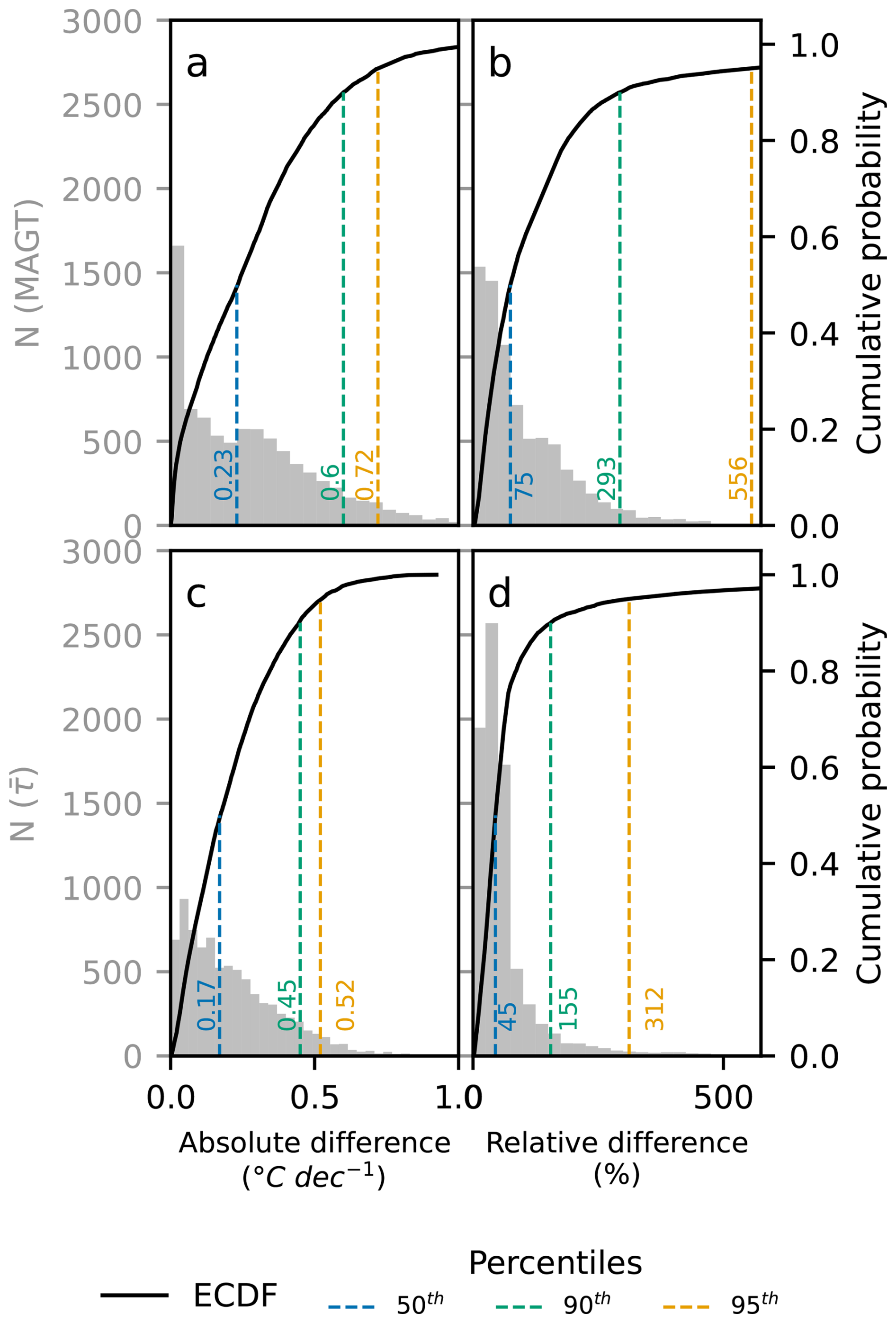
Figure 3 Sensitivity of 10-year ground temperature trends to observation depth. The magnitude of the 10-year trend is more sensitive to measurement depth for Mean Annual Ground Temperature (MAGT; a, b) than it is to the total integration depth for thermal integral ($\stackrel{\mathrm{‾}}{\mathit{\tau }}$; c, d). This relationship holds for both absolute (°C decace⁻¹; a, c) and normalized (%; b, d) differences. Grey histograms (left axis) show the distribution of trend differences for measurement depths between 10 and 20 m across all terrain types. Solid lines (right axis) represent the empirical cumulative distribution functions (ECDF) averaged over all materials. An additional supplementary figure (included in Supplementary Materials) shows individual ECDFs for each material, showing that bedrock consistently exhibits the highest sensitivity.

In summary, a difference in observation depth can introduce meaningful differences in the revealed decadal warming trends (Fig. 3). It is greater than 0.23 °C decade⁻¹ in 50 % of our simulated trend windows across all ground types. To contextualize this, Biskaborn et al. (2019) report global average warming rates of 0.39±0.15 °C decade⁻¹ in continuous permafrost and 0.20±0.10 °C decade⁻¹ in discontinuous permafrost, based on sensors that are between 5 and 24.5 m deep. The magnitude and uncertainty of warming rates presented there are commensurate with the uncertainties due to sensor position we show.

The differences of $\stackrel{\mathrm{‾}}{\mathit{\tau }}$ trends caused by integration depth are lower than for MAGT observation depths (Fig. 3c, d). Additionally, sites can be more meaningfully compared even when the sensors may not be at the same depth because $\stackrel{\mathrm{‾}}{\mathit{\tau }}$ can be interpolated to a common depth where sensors at the same depths are not available.

4.10 Directional reliability and signal to noise ratio of TSP metrics

For each TSP metric and heat content variable (H_s, H_l, and H_t), we evaluate the signal to noise ratio (SNR) and reliability of the relation. We use the regression t-statistic (i.e. coefficient estimate normalized by the standard error) and significance to measure SNR; larger percentages of significant t-statistics provide evidence of high SNR. Note that this does not tell us about the strength of the relation, but rather how much we can trust the direction and existence of change in borehole heat based on an observed change in a metric. We use the distribution of positive vs negative values to measure directional reliability; more consistently positive or consistently negative coefficients provide evidence for greater directional reliability.

For each 10-year moving window in the simulation results, we calculate a linear regression between the metric and the heat content variable. The t-statistics and levels of significance are then aggregated and summarized by the percentage of significantly positive and significantly negative coefficients. This is repeated for different levels of sensor quality (𝒬₀, 𝒬₁, 𝒬₂) and different observation lengths (5, 10, and 20 years) to describe the impact of these variables on reliability and SNR.

A detailed example for a single metric and heat variable is shown in Fig. 4. In this example, most correlations are positive. However, in as many as 2 % of 5-year windows and 4 % of 20-year windows, this correlation is negative (decreased reliability). Results for all simulations are summarized in Table 3 and the remaining figures are included in the Supplement (S1).

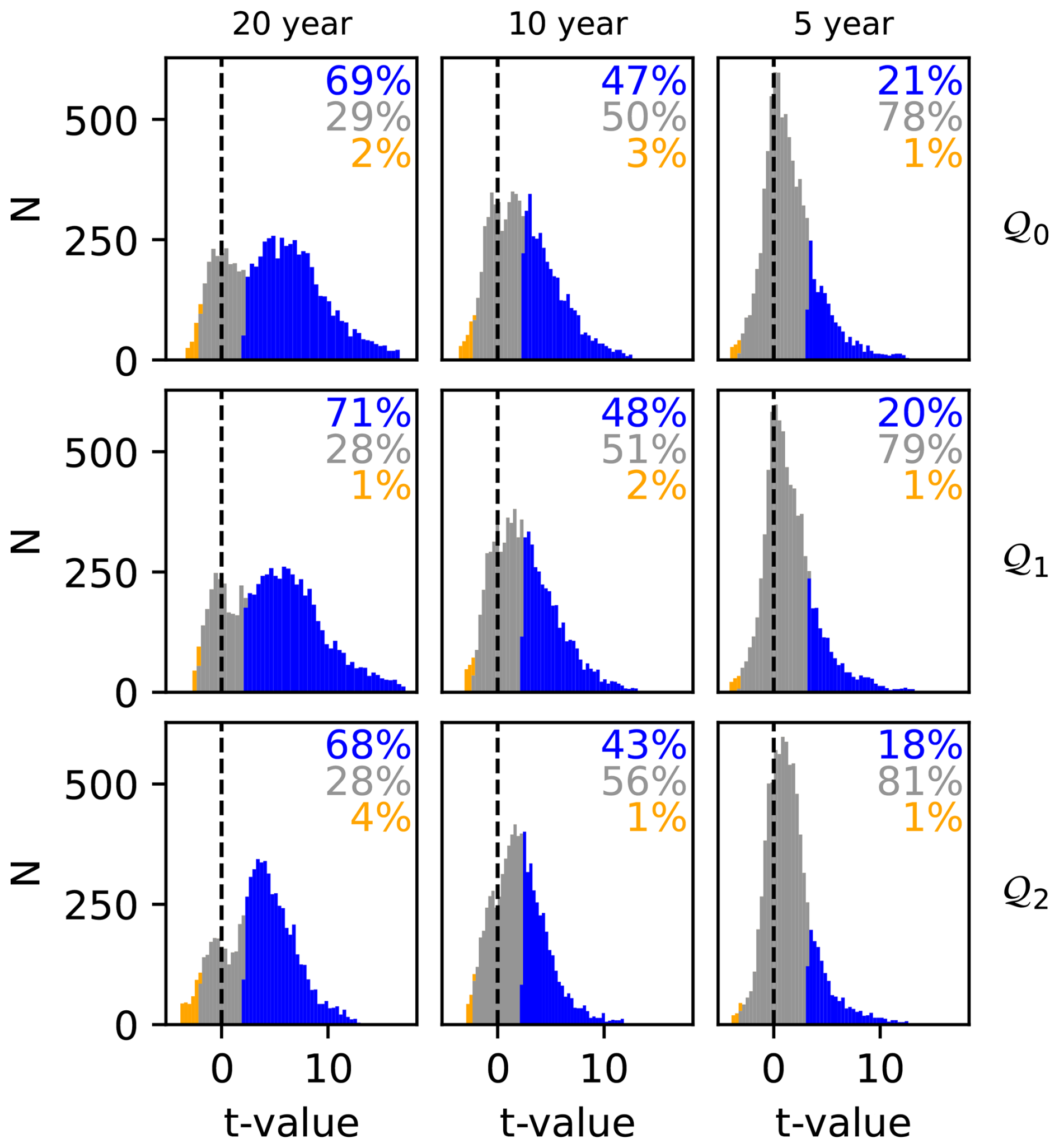
Figure 4 Effect of sensor quality and data length on the SNR of metric (T_za) – heat (H_s) relationship. Larger t-values indicate a larger SNR in the relationship between changes in metric and changes in heat content. More consistently positive or consistently negative t-values demonstrate a less ambiguous interpretation from the metric. Each histogram shows the distribution of test statistics for different averaging windows (5, 10, and 20 years) and levels of sensor quality (Table 2). Each distribution is coloured in up to three regions according to whether the regression within the window is significantly negative (orange), significantly positive (blue) or not significant (grey) at p<0.05. The percentages are included as text at the upper right corner of each panel and also tabulated in Table 3.

Table 3 Distribution of t-statistics measuring how reliably each metric corresponds to the sensible, latent, or total ground heat content for a given averaging window and data quality. Numeric values represent the percentage of significantly positive (left 9 columns) or negative (right 9 columns) relationships across all observation windows (corresponding to the blue and orange percentages in e.g., Fig. 4). Higher values in a row correspond to greater SNR; More unevenly distributed values between the left and right columns corresponds to greater reliability. A colourized version is available in the supplementary material.

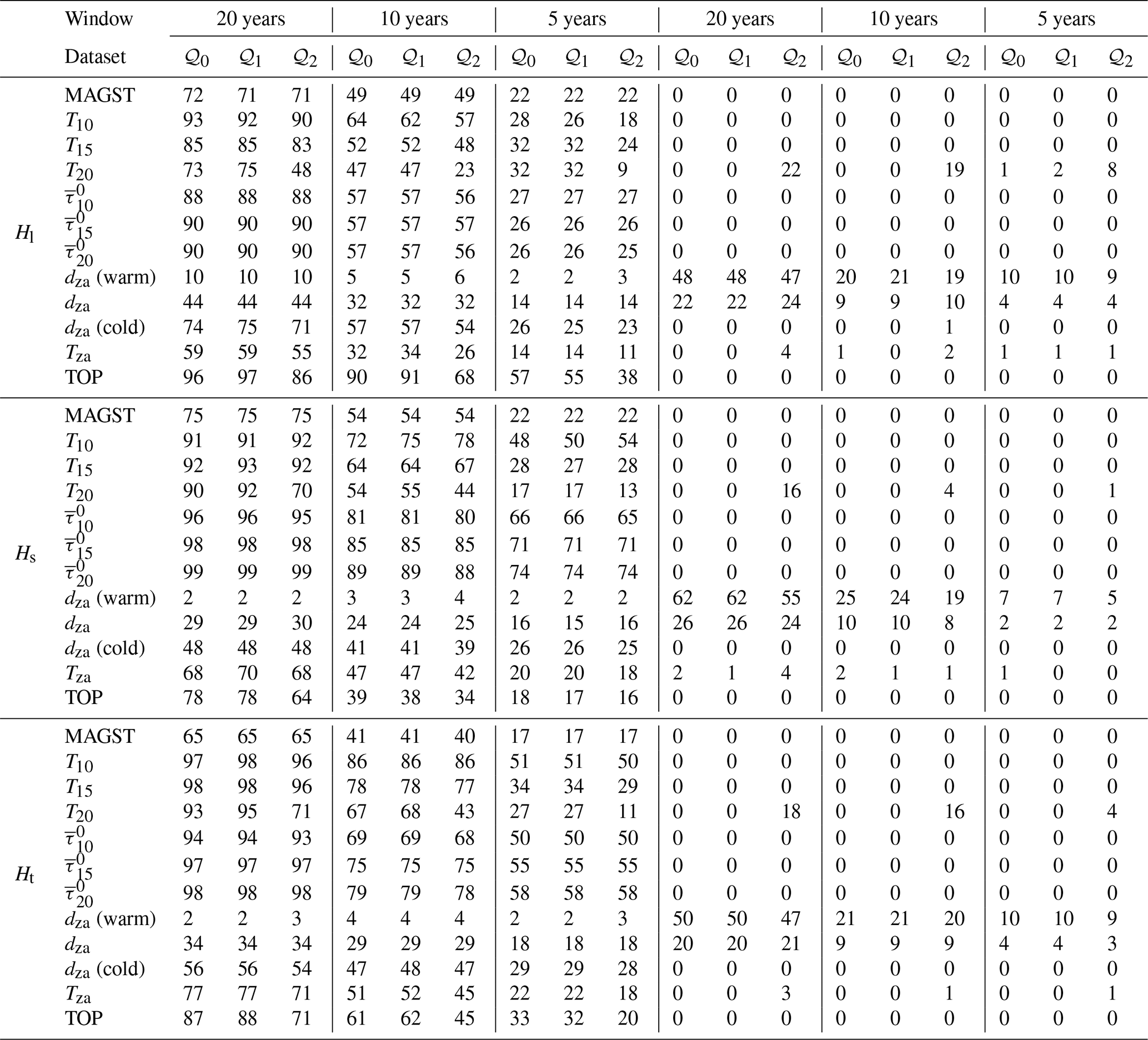
The impact of sensor quality on SNR is within a few percentage points for most TSP metrics with a few exceptions. The SNR of TOP is decreased with decreased sensor quality (most notably for 𝒬₂) for all heat variables and for all window sizes. The SNR of MAGT (T₁₀, T₁₅, and T₂₀) for H_l is also appreciably decreased with decreasing quality for 5-year windows, but not for longer window sizes. Additionally, the impact of sensor quality is greatest for larger observation depths (T₂₀).

Reliability and SNR for d_za is low overall, but when observation windows are split into warm and cold scenarios according whether t_za is above or below −0.5 °C, the SNR and reliability both increase. For cold permafrost, d_za achieves high SNR with up to 75 % significance for H_l in 20-year windows. In warm periods, d_za achieves values up to 75 % for H_l in 20-year windows. When averaged over all time windows and levels of sensor quality, metrics describing annual temperature averages (MAGT and $\stackrel{\mathrm{‾}}{\mathit{\tau }}$) rank among the highest for both H_l and H_s.

Without exception, the SNR of the metrics decreases for shorter temporal windows. Most metrics have scores of less than 30 % for 5-year windows. However, TOP-H_l is the exception, with a lowest value of 57 %. For short windows, $\stackrel{\mathrm{‾}}{\mathit{\tau }}$ has higher SNR as predictors of H_s and H_l than single-depth temperature measurements, these also score more than 50 % in 5-year windows.

The SNR of most metrics is larger for H_s than for H_l but TOP-H_l is the exception to this. Interestingly, values for H_t are not simply weighted averages of H_l and H_s: the SNR of H_t is consistently greater than either H_l or H_s for T₁₀, T₁₅, T_za; smaller for MAGST; and intermediate between the two for ${\stackrel{\mathrm{‾}}{\mathit{\tau }}}_{\mathrm{10}}^{\mathrm{0}}$, ${\stackrel{\mathrm{‾}}{\mathit{\tau }}}_{\mathrm{15}}^{\mathrm{0}}$, and ${\stackrel{\mathrm{‾}}{\mathit{\tau }}}_{\mathrm{20}}^{\mathrm{0}}$. For d_za, H_t is intermediate for 10- and 20-year windows, and greater for 5-year windows.

We interpret a higher SNR (larger number of significant values) to indicate that an increase in a given metric more reliably indicates an increase in the heat variable of interest over a randomly selected observation window. However, the time- and location-dependent relation between the metric and heat content means that we do not interpret these results in terms of the strength of the relation. Also, because we only simulate a warming trend, we generally interpret reversed correlations as a consequence of one of three factors: interannual variability, temporal window mismatches due to time lags, and errors due to decreased sensor quality. For example, the negative correlations in Fig. 4 would not be caused by an increase in the metric when H_s decreases within the window, but rather by a decrease in the metric (for one of the three reasons stated above) as the H_s increases.

In general, we see that our sensor imperfection model results in only a small effect on the effectiveness of metrics as predictors, except for short observation periods. For MAGT, we expect the effect of normally distributed noise is likely erased in individual sensor records because they are averaged over the year. We expect the bias and trend in 𝒬₂ also contributed to the lower performance.

Averaging multiple sensors in the calculation of $\stackrel{\mathrm{‾}}{\mathit{\tau }}$ would also reduce the impact on the metric of sensor drift and bias in any individual sensor. On the other hand, the calculation of annual maxima required to estimate TOP relies on single data points and involves no averaging – this would be directly affected by sensor bias and noise. This would therefore more strongly affect metric performance by amplifying, rather than dampening, the effect of deviations from the perfect model data. d_za also requires additional calculations, but the performance of this metric is not similarly affected; the method by which it is calculated also averages amplitude data from multiple sensors.

The large impact of decreased sensor quality on T₂₀ which shifts the results towards a negative correlation may illustrate a weakness of the methodology which is that we only perform a single realization of the randomized sensor quality model. In this case, it may be that the realization produced significantly more negative trends at that depth. Alternatively, it is possible that the sensor bias and drift have a larger effect because the signal magnitude is much smaller at that depth.

d_za exhibits a different signal than other metrics (Fig. 1c, i). However, the reliability is low, especially for short observation windows (Table 3). We attribute this to the noisy nature of the metric, the period of stagnation prior to the reversal of the trend and the temperature-dependence of the metric overall. The higher interannual variability means that longer temporal windows are needed to obtain clear trends. More importantly, the results highlight the importance of defining a precise cutoff at which the behaviour of d_za reverses.

$\stackrel{\mathrm{‾}}{\mathit{\tau }}$ is a better indicator of H_s and H_t change over shorter observation periods than MAGT (e.g $T_{\mathrm{20}},T_{\mathrm{15}},\mathrm{\dots }$). This is in spite of the greater interannual variability of $\stackrel{\mathrm{‾}}{\mathit{\tau }}$ caused by the inclusion of near-surface measurements. Intuitively, we expected this variability to make trends harder to predict. We believe that this effect is outweighed by the diminished impact of latent heat in warm conditions, which causes MAGT trends to become greatly diminished. It is also interesting to note that although qualitatively $\stackrel{\mathrm{‾}}{\mathit{\tau }}$ behaves similarly to a superimposition of MAGST and MAGT, both of those metrics are more strongly affected by shorter observation windows. We interpret this to mean $\stackrel{\mathrm{‾}}{\mathit{\tau }}$ benefits from being depth-integrated, which more closely resembles how H_s would be calculated if heat capacities were known.

4.11 Summary of insights from testing TSP metrics with simulation experiments

MAGT is traditionally the most widely used metric to report permafrost change. It is a direct measurement of the permafrost and it reveals how quickly the permafrost thermal state is changing at a specific depth. Trends correlate well with column heat contents, but the relationship is time-,depth-, and location-dependent. As a consequence, comparing (between locations or times) and aggregating MAGT trends usually involves blending dissimilar physical processes, producing a number with no meaningful connection to either heat gain or ice loss. Therefore, MAGT trends are most useful for detecting the presence and sign of a trend. The metric is also prone to periods of imperceptible change, making quantification difficult.

$\stackrel{\mathrm{‾}}{\mathit{\tau }}$ is a good indicator of changes in borehole sensible heat (H_s), already over shorter time periods, outperforming MAGT in this regard. It is less prone to stagnant behaviour, making trend detection more reliable. It also takes advantage of all available sensors. Practically, it allows for compensation of unequal monitoring depths through standardized integration, improving comparability between boreholes. While being subject to the same limitations as MAGT in principle, the confounding effects of latent heat on the ability to compare or aggregate trends are reduced for $\stackrel{\mathrm{‾}}{\mathit{\tau }}$.

Despite the common definition of MAGT as the temperature at d_za, we find little support for using T_za as a TSP metric to monitor permafrost change. In addition to the greater complexity of calculating this metric, it is the first one to become isothermal in the simulations as the ground warms. It is also less predictive of column heat content compared to MAGT or $\stackrel{\mathrm{‾}}{\mathit{\tau }}$ (Fig. 3). However, it may be useful for (1) indicating near-isothermal behaviour in a borehole because it will be the first metric to achieve this, and (2) as a classifier for late-stage permafrost thaw; in our simulations, the point at which T_za reached approximately 0 °C coincided with the transition in sign of the d_za-warming relation.

TOP is a straightforward metric for temperature-based monitoring with a clear physical meaning, describing changes in permafrost thickness. It behaves similarly to ALT or $\stackrel{\mathrm{‾}}{\mathcal{D}}$ but with some clear advantages. The definition of TOP is purely thermal and less ambiguous than that of ALT, which is alternatively defined based on temperature or phase state (van Everdingen, 1998; Burn, 1998). Additionally, the direction of ALT trends reverses after the formation of a supra-permafrost talik while TOP remains monotonic. Although $\stackrel{\mathrm{‾}}{\mathcal{D}}$ may have inherent meaning, it is qualitatively similar enough to TOP that there is little to gain by including both in a parsimonious set of metrics. Adopting TOP as a primary metric also does not diminish the utility of existing ALT records and monitoring programs; in the absence of a talik, TOP can be considered equivalent to the purely thermally defined ALT.

Overall, TOP is a good proxy for H_l even in short time windows, even though the exact correspondence is unknown without quantification of ice content. In our simulations, it increases slowly in the early stages of warming and then accelerates in later stages of warming. TOP has an easily understood physical meaning, describing a change directly affecting permafrost thickness. However, the accuracy with which it can be estimated is more strongly affected by sensor spacing (e.g., Riseborough, 2008) and quality than other metrics. Some confounding may originate from subsidence caused by a rising permafrost base.

d_za can be used to infer changes to H_l, but it provides an incomplete picture: phase change below d_za is invisible, the upper limit of d_za is affected by the choice of cutoff for “zero amplitude”, and the sign of the correlation between d_za and H_l is temperature-dependent. However, the behaviour of the metric is qualitatively distinct from ground temperature, which can be helpful in interpreting permafrost changes.

Given the above results, we recommend TOP, d_za, and $\stackrel{\mathrm{‾}}{\mathit{\tau }}$ in addition to MAGT as a parsimonious set of metrics for quantifying permafrost change. MAGST can be considered as an additional metric that, while not observed in permafrost, provides the clearest measure of how climate or disturbance drive changes at depth.

5 Case study with observations from GTN-P

As a demonstrator with field observations, we calculated TSP metrics for selected ground temperature records from the GTN-P database. Data were downloaded for all boreholes with available temperature time series. 38 sites met our initial criteria: (1) at least 5 years of data; (2) at least daily measurement frequency; (3) a maximum observation depth of at least 5 m; and (4) at least 5 depths of observation. After manual removal of datasets with excessive noise or data gaps, only 14 boreholes from 10 areas were retained; 9 areas were located within the European Alps, and one within Russia (map of sites included in supplementary material as Figure S37). Finally, three boreholes – Samoylov, Ritigraben (RIT_0102) and Schilthorn (SCH_5198) – were selected. Samoylov is located in Russia's Lena River Delta and is within the continuous permafrost zone. The two Swiss sites are located in warmer mountain permafrost. Data for the latter two sites were supplemented with more recent observations from PERMOS (Swiss Permafrost Monitoring Network, 2024). Metrics and trends were calculated for all three sites based on at least 15 years of data (Fig. 5).

At Samoylov, the observed warming rates of 2.9 °C decade⁻¹ at 9.75 m and 1.6 °C decade⁻¹ at 20.75 m are high, consistent with cold permafrost. The difference in calculated decadal warming rates between the two observation depths is also high at 1.1 °C decade⁻¹ (a 54 % difference). Warming rates at the other two sites are much lower. At RIT, there is no detectable warming trend at 10 m and at SCH, the warming rate is 0.3 °C decade⁻¹ at 13.0 m: typically low for warm permafrost.

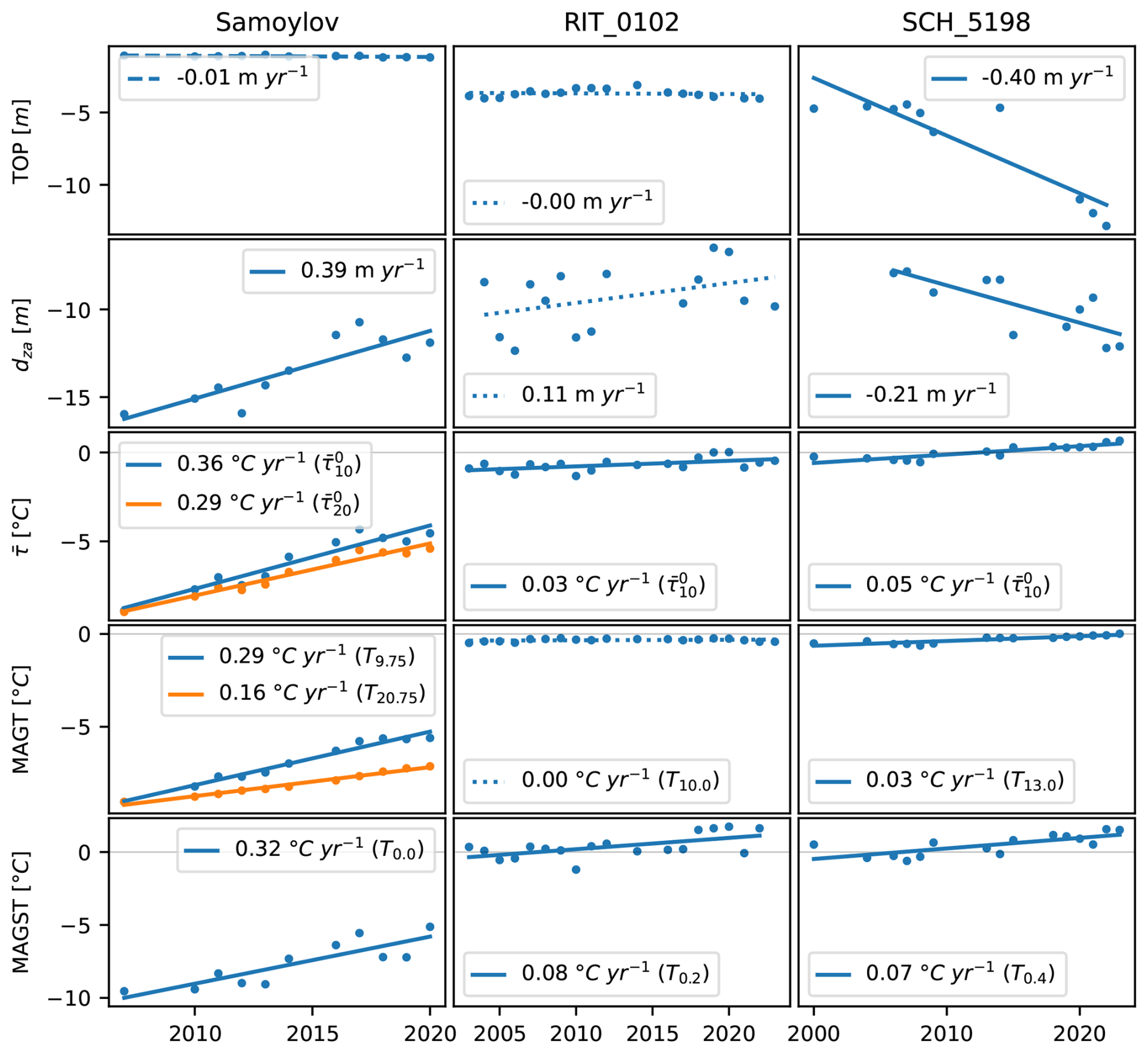
Figure 5 Selected TSP metrics calculated for three GTN-P monitoring boreholes. Solid trend lines are significant at p<0.05, dashed trend lines are significant at p<0.1, and dotted trend lines have p≥0.1. Where appropriate, depth information is included in each figure legend.

The MAGST trend at Samoylov is consistent with warming at depth and has a similar magnitude. In contrast, MAGST warming rates at the warmer sites are markedly higher than the MAGT rates. The greater difference between warming at the surface and warming at depth is another indication that latent heat at depth reduces the observed MAGT change.

Surface warming rates at all sites are high relative to published values of e.g., ca. 0.2–0.6 °C decade⁻¹ (Hu et al., 2019; Wu et al., 2012; Swiss Permafrost Monitoring Network, 2024).

While there are no published $\stackrel{\mathrm{‾}}{\mathit{\tau }}$ observations with which to compare these trends, they can be meaningfully compared to either MAGST or MAGT trends. $\stackrel{\mathrm{‾}}{\mathit{\tau }}$ increases at Samoylov at a rate between 2.9 °C decade⁻¹ (20 m integration depth) to 3.6 °C decade⁻¹ (10 m integration depth). At two warmer sites, ${\stackrel{\mathrm{‾}}{\mathit{\tau }}}_{\mathrm{10}}^{\mathrm{0}}$ increases relatively slowly: by 0.3 °C decade⁻¹ at RIT and by 0.5 °C decade⁻¹ at SCH.

At RIT, estimated TOP change rates (0 cm yr⁻¹) do not provide any indication of change. At Samoylov, a change rate of −1 cm yr⁻¹ is modest relative to observations elsewhere (e.g., Smith et al., 2022) and low when compared to the degree of thermal change taking place. However, at SCH we observe rates of −40 cm yr⁻¹ which is among the highest observed rates globally. This also is in contrast to the modest warming signals seen at the site.

At each site, we observed changes to d_za during the observation period. At Samoylov and RIT, d_za is becoming shallower, consistent with the first phase of warming and indicative of greater freeze-thaw activity. d_za change is slightly greater at Samoylov (+3.9 m decade⁻¹) compared to the warmer RIT (+1.1 m decade⁻¹). At SCH, the magnitude of d_za change is greatest (−2.1 m decade⁻¹) and its direction has changed, consistent with late-stage warming found in our simulations.

The use of multiple TSP metrics allows us to better quantify interpret permafrost change. At Samoylov, three out of three temperature-based metrics indicate rapid warming. We do not observe the characteristic reduction in warming rates caused by latent heat, but nevertheless we can infer from rising d_za that there is increased freeze-thaw taking place in the ground.

At RIT, MAGT changes are not detectable. Additionally, there is no detectable trend in TOP over the observation period. Taken in isolation, these key metrics suggest little change is taking place. When we consider MAGST and $\stackrel{\mathrm{‾}}{\mathit{\tau }}$, we are better able to quantify temperature change. Finally, the moderately high rate of d_za change alongside the muted temperature signal provides quantifiable evidence of changes to latent heat in the ground.

At SCH, two out of three temperature-based metrics indicate slight warming and one indicates moderate warming. TOP is changing rapidly. The deepening d_za shows that the site is in a late stage of warming and permafrost degradation, likely associated with talik growth.

6 Discussion

6.1 Testing TSP metrics with simulated data

Simulations represent an ideal scenario with which to evaluate the metrics but they can only provide some of the complexity of the real environmental system. In practice, heterogeneous subsurface characteristics will mean observations at an individual depth are less well representative of permafrost above and below. Spatially variable ice content will amplify or dampen the response of these metrics to thaw, and this will affect rates of change. Instrumentation density has a major impact on the accuracy and precision of many metrics (e.g., Hinkel, 1997) and will affect the resolution with which some of the metrics can be calculated.

Representing change as a single per-borehole statistic is challenging because of differences in data completeness and measurement density in boreholes. Observational records in boreholes differ in their vertical extent and duration. Averages can therefore mask locations with strong change when boreholes are very deep or have many sensors or exaggerate measures of change in boreholes with few sensors.

6.2 Model limitations

Our use of FreeThaw1D means we do not consider spatial effects or the soil water balance. Taken together, these limitations could affect our results and the applicability of the metrics.

Advective water transport could lead to local redistribution of heat that does not correspond to an overall net change in the larger area. This could lead to an overestimation of change by the metrics because they only measure local changes.

In our simulations, there is also no water flow within or out of the simulation with the exception of melted excess ice. Temporal variability in near-surface moisture can influence d_za by altering the soil’s apparent thermal diffusivity independent of long-term change. The model’s fixed moisture conditions may smooth out these variations, leading to more stable d_za trends than would occur in reality. This may cause d_za to appear less sensitive to changes in H_l than it truly is.

This lack of water flow also means that during late-stage thaw in warm, icy simulations with a supra-permafrost talik, the d_za becomes shallower than the top of permafrost, and is kept shallow by the buffering effect caused by freeze-thaw cycles of supra-permafrost water. It is plausible that an overall loss of moisture above the permafrost table during this period could prevent the d_za from ever reaching the top of permafrost, or alternatively accelerate the late-stage shallowing of d_za.

Despite these potential biases, our focus on the relative performance across metrics helps control for systematic errors. For example, if all metrics are similarly affected by missing processes advection, their relative performances remain valid.

6.3 Interpretability of MAGT trends

Our results show that increasing MAGT is consistently indicative of increases in column H_l and H_s even in the presence of distortion from sensor noise, bias, and trends. However, the exact quantitative relationship is location- and time-dependent. In this regard, it may be the direction of the trend from which meaning can be most unambiguously derived. However, given that the vast majority of permafrost boreholes are warming (Biskaborn et al., 2019), this may be an almost trivial conclusion.

Our results suggest that MAGT can contribute to a descriptive picture of permafrost change, but only when used in combination with other temperature-derived metrics. In isolation, the magnitude of MAGT trends can be attributable to both the effect of latent heat and the intensity of surface warming. With a more complete suite of indicators, the effect of latent heat can be made more explicit and permafrost change can be quantified more reliably.

Our results highlight the challenges of comparing trends between boreholes or regions. In our simulations, the behaviour of each metric generally follows a similar trajectory. For MAGT, this is: rapid warming, reduced warming, no warming, and finally rapid warming if thaw progresses to the observation depth. Most importantly, we do not change the magnitude of the warming trend at the surface, yet the trends measuring permafrost response show a great deal of variability across simulations and at different points in time. Therefore, in our experiments, MAGT tells us more about the configuration of the system and the stage of thaw than about the intensity of the warming trend. In this regard, the resolution of MAGT as a climate indicator may indeed be limited to the trend direction discussed above. In reality, locations will be subject to different trends in air temperature, snowpack and vegetation; all of which will affect warming rates at depth. However, this signal will be superimposed on the purely permafrost-dependent variability which, as we have shown, is on the same order of magnitude as observed trends.

Our results also provide some guidance on how to make MAGT trends more interpretable. If we are interested in understanding where permafrost change is happening faster or more slowly, groupings should account for both the ground conditions and some other indicator of the stage of warming. We show that T_za is a good candidate for this. The breakpoint in the T_za trend is able to separate warming into two stages with statistically distinct trends in H_s and H_l. The performance of the T_za breakpoint is superior to the traditional classification of warm permafrost (MAGT $>-\mathrm{2}$ °C) which does not discriminate H_s trends in the two stages. This is significant because H_s trends are strongly linked to temperature. This approach also has the advantage that T_za often requires only relatively shallow observations because d_za becomes shallower as the borehole warms.

Current comparisons and aggregations of MAGT trends are most commonly grouped by region or permafrost zone. This partially accounts for temperature and warming stage, but this is hampered by uneven and biased spatial sampling, particularly in the discontinuous permafrost zone where permafrost temperature may still be strongly affected by surface conditions. In these cases, more meaningful comparisons could be made by further subdividing datasets according to the ground conditions on a spectrum of ice content. However, such fine-scale subdivision may be limited by general lack of ground temperature data and result in too few boreholes in each category to meaningfully compare.

6.4 Permafrost metrics as a climate indicator

Despite its application as a climate indicator, permafrost temperature change is complicated by the effects of latent heat and we should expect permafrost warming rates to diminish as boreholes approach 0 °C. One possible solution is to consider using only boreholes with very little ice content, as would be expected in certain kinds of bedrock. Such an approach has been suggested by Smith and Riseborough (1996), who recommend monitoring in exposed bedrock to obtain the most direct climate signal from ground temperatures. The PACE project provides another example where boreholes in bedrock on mountain summits or plateaus were used for permafrost and climatic monitoring (Etzelmüller et al., 2020; Harris et al., 2009). In general, however, bedrock sites remain underrepresented in much of the permafrost monitoring data because of difficult drilling conditions, and because permafrost impacts are often caused by thaw of ice-rich ground.

6.5 Temperature-dependence of d_za trends

Changwei et al. (2015) also show observations of reversing d_za behaviour and explain this behaviour with an equilibrium model (i.e., analytic heat conduction equation with a sinusoidal surface temperature variation). However, a limitation of this approach is that the transition in correlation sign cannot be examined – their warm, deep-d_za simulation only exists as a fully thawed profile rather than one with dynamic behaviour. Our transient simulations show that this reversal can take place over several years during which the d_za changes very little and the sign of the correlation between d_za and air temperature is undefined.

This distinction is important because other studies report unidirectional (and conflicting) relationships between warming trends and d_za (e.g. Bonnaventure et al., 2015; Wang et al., 2022). An important next step in this approach to monitoring will be developing additional criteria to more clearly delineate when a positive- or negative- correlation should be assumed.

6.6 Talik development and accelerated permafrost degradation

We observe accelerated degradation (lowering of TOP) in warm permafrost as it becomes isothermal and develops a supra-permafrost talik. Similar discrepancies have been described elsewhere. On the Tibetan Plateau, ALT deepening rates have been shown to be greater in warm permafrost than in cold permafrost (Changwei et al., 2015). In discontinuous permafrost and peatlands, taliks have been described as giving rise to tipping-point behaviour and kicking off rapid degradation (e.g., Connon et al., 2018; Devoie et al., 2019). We observe this phenomena across different stratigraphic types (Table B1) and climates, representing a wide range of permafrost conditions, suggesting a greater abundance of this tipping point behaviour than may have previously been considered.

Certain TSP metrics may offer insight as to when this accelerated degradation may occur. In our simulations, it is preceded by the breakpoint in T_za and the halting of the d_za shallowing trend. These can act as quantifiable indicators that permafrost is in late-stage thaw and that subsequent talik formation and rapid degradation are imminent.

6.7 Implications for monitoring

Such rapid change could affect permafrost monitoring efforts by causing TOP to descend rapidly out of the measurement range of existing thaw tube installations (O’Neill et al., 2023). As a solution, movable thermistor chains with dense spacing near the permafrost table may help capture changes in TOP, and records of subsidence (Gruber, 2020) may inform estimates of excess ice loss. Similarly, methods of observing and reporting ALT may benefit from adjustments to remain relevant even with talik formation.

7 Conclusions and recommendations

We investigated the long-term behaviour of a suite of temperature-derived metrics as indicators of permafrost thaw. Our results suggest that calculating multiple temperature-derived TSP metrics provides rich information for characterizing and understanding permafrost change, particularly in warm permafrost. More specifically:

• In addition to MAGT, we recommend TOP, d_za, $\stackrel{\mathrm{‾}}{\mathit{\tau }}$, and MAGST as a parsimonious set of five metrics.

• The suitability of individual metrics as indicators of change varies through time in the simulations. While most experience periods of time with no change, the exact timing of these periods differs between metrics.

• We find that a multi-metric approach to permafrost monitoring makes it possible to identify and quantify change in isothermal boreholes during periods where MAGT and ALT trends are negligible.

We also quantify the impact of observation depth on MAGT trend rates and find:

• Differences in the depth at which MAGT is reported results in differences in 10-year warming commensurate with both the magnitude and uncertainty of warming rates reported elsewhere. This effect is strongest in soil with little moisture content.

• Warming rates of the thermal integral ($\stackrel{\mathrm{‾}}{\mathit{\tau }}$) are slightly less affected by differences in integration depth.

Our results also suggest caution when using change in permafrost metrics as broader climatic indicators, especially when considered in aggregate:

• Wide variability in observed trends is possible even in the absence of differing climate signals because of the time- and material-dependent response of the metrics.

• While metrics can be used as an indicator of warming vs. cooling, even the sign of the climate-metric relationship can change over time.

• Quantitative comparison and aggregation of trends from multiple locations or multiple times (acceleration and deceleration of change) likely produces results with no meaningful connection to heat gain or ice loss.

Appendix A: Symbolic notation

T	temperature	°C
t	time	days
z	depth	m
dza	depth of zero annual amplitude	m
Tza	temperature at dza	°C
TDD	thawing degree days	°C day
FDD	freezing degree days	°C day
$\stackrel{\mathrm{‾}}{\mathit{\tau }}$	thermal integral	°C
$\stackrel{\mathrm{‾}}{\mathcal{D}}$	annual thaw-depth duration	m3 m−2
λs	thermal conductivity of	W m−1 K−1
	soil particles
cs	specific heat capacity of	J m−3
	soil particles
ℋ	heat transfer coefficient	W m−2 K−1
θsat	Van Genuchten saturated	m3 m−3
	water content
θres	Van Genuchten residual	m3 m−3
	water content
α	Van Genuchten parameter	m−1
n	Van Genuchten parameter	–
ϵ	Excess ice content	m3 m−3

Appendix B: Model setup and validation

We use the model FreeThawXice1D (Tubini and Gruber, 2025; Tubini et al., 2021) to simulate ground conditions. This model version represents the effects of ground subsidence caused by ice loss within the ground and accurately tracks zero-degree isotherms via local mesh refinement.

B1 Model input and initial conditions

The model is driven by meteorological forcing data obtained using GlobSim (Cao et al., 2019). This tool streamlines the download of reanalysis data, interpolates grid cells to point-scale to make data suitable for 1D simulation, standardizes units and timesteps, and performs heuristic downscaling to account for terrain and other local effects.

We use data from the ERA5 reanalysis to create three sets of meteorological forcing data (1980–2022). One is for Yellowknife, Canada (62.45° N, 114.4° W), one is for a area near Lac de Gras, Canada (64.7° N, 110.4° W), and the last one is for Tombstone Territorial Park in Yukon, Canada (64.56° N, 138.43° W).

For model spin-up, we repeat the first three years of input data. First, the model is run for 300 years with a 40 m total depth. Next, the deep temperature is extrapolated to 150 m using the geothermal heat flux. The remaining model runs use the 150 m total depth.

Future conditions are simulated by repeating the last 5 years of input data and changing values using climate projections from Climatedata.ca (Cannon et al., 2015) based on the SSP5-8.5 scenario. We calculate the change in projected annual mean temperature for an arbitrary year relative to the final year of reanalysis data and add this difference to the corresponding year of input data. To simulate different ground conditions, we create five distinct stratigraphies (Table B1).

Table B1 Stratigraphy definition for four simulation locations.

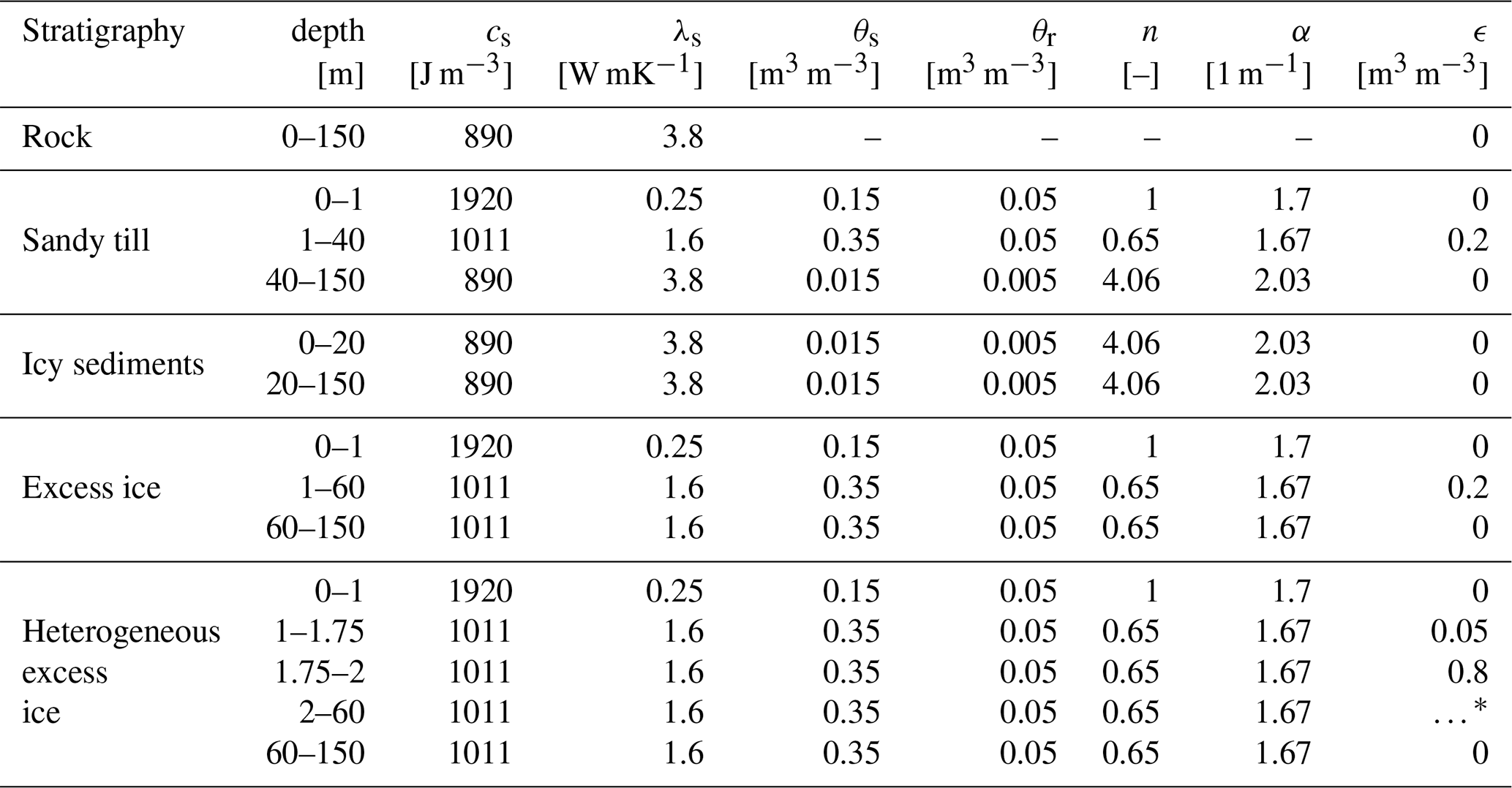
Values chosen based on (Dall'Amico et al., 2011; Tubini et al., 2021). ^* Alternating values of 0.05 and 0.8 are repeated using the same distribution as the second and third layers.

B2 Atmosphere-ground coupling

The effects of surface conditions and surface cover such as vegetation and snow are represented with the heat-transfer coefficient ℋ [$\mathrm{W}{\mathrm{m}}^{-\mathrm{2}}{\mathrm{K}}^{-\mathrm{1}}$]; for a medium of finite thickness such as a snow pack, ℋ would be derived as a thermal transmittance. In equilibrium, it is the inverse of thermal resistance and with oscillating temperature conditions, it may be reduced due to temporary storage and release of heat by the medium characterised (Tubini and Gruber, 2025). During summer, we use a constant value, ℋ_s and during winter, it is parameterized as a function of the daily snow water equivalent ℋ_w.

Snow-water equivalent (SWE [m]) is computed from daily accumulation and ablation. Snow is accumulated at the rate of daily precipitation for days with a mean air temperature below a threshold of 2.8 °C (e.g., Kienzle, 2008). Snow melts based on a degree-day model (e.g., Rango and Martinec, 1995) whereby SWE is lost at a rate of 3 mm ${\mathrm{K}}^{-\mathrm{1}}{\mathrm{d}}^{-\mathrm{1}}$ when mean daily air temperature is above 0 °C.

Snow thermal transmittance is computed from SWE, a proportionality coefficient γ [m K W⁻¹] translating SWE into an R-value, and an aging function β [days] reflecting densification over time t [days]. To ensure ℋ_w does not become large without bound as the snowpack thins, we also impose a maximum value (ℋ_max) which is also used for snow-free conditions:

$$\begin{array}{}\text{(B1)}& {\mathcal{H}}_{\mathrm{w}}\left(\mathrm{SWE}\right)=max\left({\displaystyle \frac{\mathrm{1}}{\left(\mathrm{SWE}\right)\mathit{\gamma }(\mathrm{1}-\frac{t}{\mathit{\beta }})}},{\mathcal{H}}_{\max }\right).\end{array}$$

The coefficient γ has a physical basis for individual snow layers (Fig. B1) and is extended here as a parameter characterizing an entire snow pack. In representing for example, taiga and tundra snow packs, γ will parameterize typical conditions such as density and the effect of layering.

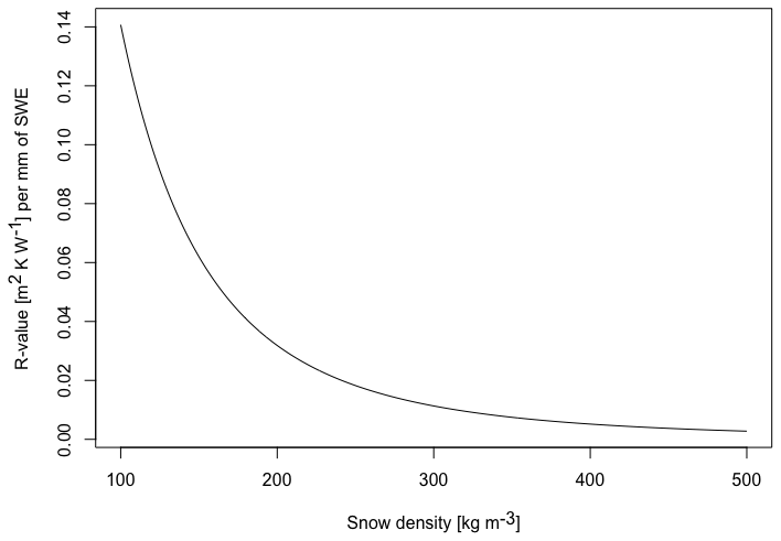
Figure B1 R-value of a snow layer with 1 mm water equivalent, computed with a relationship of snow density and effective conductivity (Fourteau et al., 2021, Eq. 18 for 263 K).

B3 Model calibration

To calibrate the simplified snowpack model, we compare model results to ground temperature observations and adjust parameters to ensure that the results are plausible. We use observational data from borehole NGO-DD-2015, a study site in the Northwest Territories located at (64.703° N, 110.440° W) (Gruber et al., 2018b, a).

B4 Simulation

Using the input data described above, the model is spun-up from an initial temperature of −3 °C using repeated data (1980–1982), then run until 2100. For the purpose of evaluation, we use output for the period 2016–2021 at which time observations are available. For testing the thaw metrics, we use output for the period 1980–2100.

A set of simulated temperatures are recorded at depths corresponding to the recommended sensor spacing from the PACE Project (Harris et al., 2009) up to a depth of 15 m (i.e., at 0.2, 0.4, 0.8, 1.2, 1.6, 2, 2.5, 3, 3.5, 4, 5, 7, 9, 10, 11, 13, 15, 20, and 25 m). In practice, few monitoring locations will have this level of instrumentation.

B5 Model Evaluation

Using our simplified snowpack model, we are able to replicate the ground temperature observations reasonably well (Fig. B2), corresponding with our intent of generating plausible transient ground-thermal regimes. There is some deviation from observations, notably in 2021, although we primarily attribute this to the ERA5 data overestimating winter precipitation or air temperature. Our calibrated snow parameters are (β=365 d, γ=20 mK W⁻¹, ℋ_max=15 W m⁻² K⁻¹).

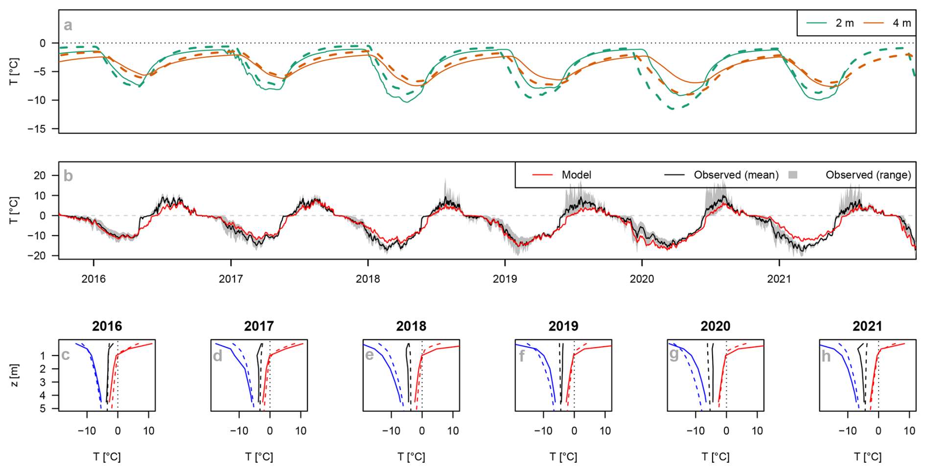
Figure B2 (a) Comparison of simulation results (dashed lines) with observations (solid lines) at selected depths (b) Comparison of simulated ground surface temperature (red) with observed mean ground temperature (black line) for 4 sensors in a 15 m × 15 m study plot. Grey shaded polygon shows total range. (c–h) Comparison of simulated (dashed line) and observed (solid line) temperature profiles for 2016–2021.

B6 Plausibility of simulated trends

We compare our simulation results with observed warming rates. These results are not intended to be interpreted as predictions of future permafrost warming. Rather, we perform this evaluation to ensure simulations are plausible in comparison with observed behaviour. First, we estimate yearly warming rates for MAGT at 13 m (Fig. B3).

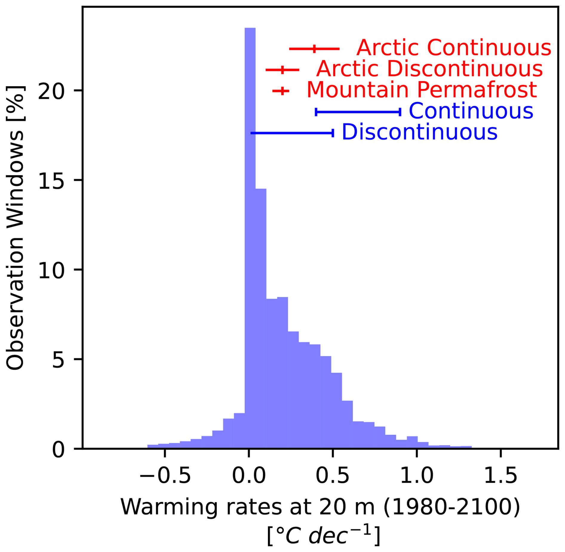
Figure B3 Histogram of warming rates at 20 m as a percentage of all possible 10-year observation windows all years across all simulations. Red intervals correspond to the mean (midpoint) and confidence interval of warming rates reported by Biskaborn et al. (2019) for different permafrost zones. Blue intervals correspond to ranges of warming rates reported in Smith et al. (2022) for different permafrost zones.

Warming rates in our simulations are distributed with a peak near 0 °C decade⁻¹ and the majority of values between 0 and 0.6 °C decade⁻¹. These values include the means and confidence intervals for average warming rates reported by Biskaborn et al. (2019). Smith et al. (2022) reports maximum observed warming rates of between 0.7 and 0.9 °C decade⁻¹ in various high-latitude regions of continuous permafrost. These values are also consistent with our simulations, although some of our simulations exhibit periods with greater warming rates; we attribute these to both the nature of the bedrock simulations, which have little water to buffer temperature changes, and to the fact that we are simulating a much longer period which extends well into the future with a moderately strong warming trend. We also observe some negative warming rates which we also attribute to our bedrock simulations which are both more susceptible to short-term temperature changes and under-represented in permafrost monitoring. The peak of the histogram corresponds to warming rates near 0 °C. Low warming rates (< 0.1–0.3 °C decade⁻¹) are commonly observed in zones of warm permafrost (Smith et al., 2022). The relatively higher proportion of periods with such low rates in our simulations is also attributed to the long simulation duration and the eventual development of near-isothermal conditions in the ground for simulations with high ice contents.

Appendix C: Emulating typical sensing systems

Table C1 Sensor accuracy, resolution, and drift from manufacturer websites.

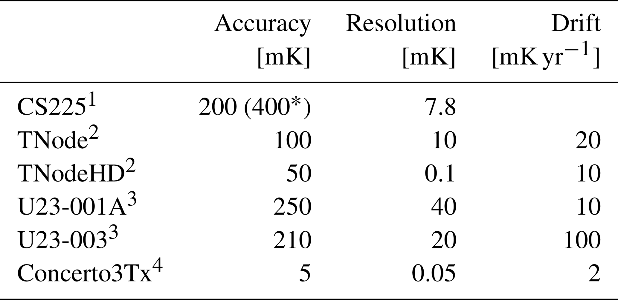
¹ https://campbellsci.ca/cs225. ² https://thermistor-string.com/index.php/string-features#specs. ³ https://onsetcomp.com/products/data-loggers/u23-004. ⁴ https://rbr-global.com/products/standard-loggers/thermistor-strings/. All web links last accessed 1 October 2024. ^* Worst-case scenario including lifetime drift.

In generating degraded data sets for emulating typical sensing systems (Table C1), we account for accuracy, drift, and precision for each sensor (simulation output depth). Accuracy limitations are modeled as a constant bias drawn from a uniform distribution (± 0, 50, 150 mK). Drift is modeled as a linear trend with a slope drawn from a uniform distribution (± 0, 1, 10 mK yr⁻¹). Precision is modeled as temporally uncorrelated normally distributed random noise (σ=0, 10, 50 mK).

Sensor accuracy of commercial systems is commonly self-reported between ± 0.005 and ± 0.4 °C. Hasler et al. (2011) estimate relative sensor accuracy to be within ± 0.3 °C.

Sensor drift is reported by manufacturers between 0.002 and 0.1 °C yr⁻¹, whereas studies under laboratory conditions give much lower rates (Lawton and Patterson, 2002). However, drift is thought to also be caused by water ingress and corrosion under field conditions or by the aging of reference resistors in logging systems. Nonlinear drift has been reported in observations; Boike et al. (2018) observe a jump of 0.5 °C over the course of a year following two years of stability and Luethi and Phillips (2016) report that drifts increase exponentially with time.

Sensor resolution (precision) reported by manufacturers ranges from 0.05 mK to 63 mK. This value determines the smallest detectable change using the sensor. Widmer et al. (2023) estimated an average noise standard deviation for sensors around 5 mK (digital band-gap) and 0.03 mK (analog resistance thermistor). Batir et al. (2017) measured standard deviations around 14 mK for deep, thermally-stable sensors.

Appendix D: Determination of exact active-layer thickness from model output

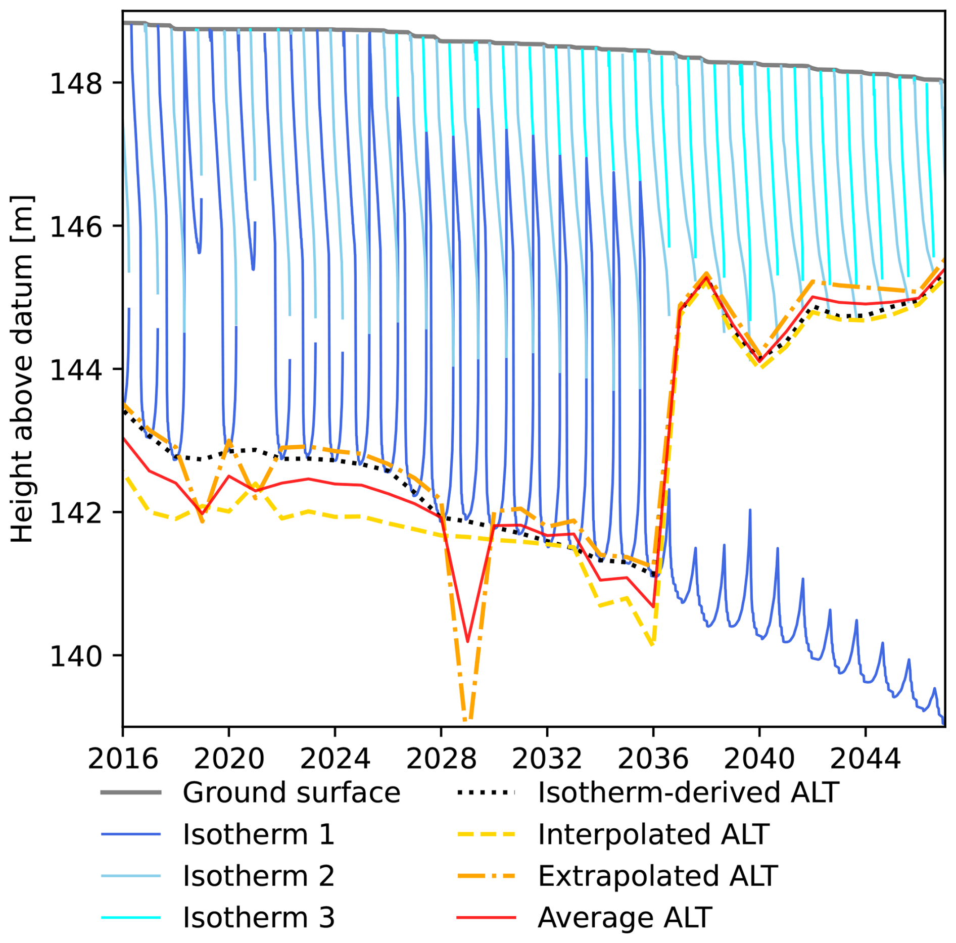
Figure D1 Example of the estimation of ALT from simulated zero-degree isotherms (blue lines) and from T(z,t) model output alone (red and orange lines). This method is able to discriminate the development of supra-permafrost taliks, as shown in the years 2036–2038. However, results occasionally differ from what is expected using a purely visual inspection. For example in 2019 and 2021, the penetration depth of that year's thawing isotherm is much shallower, but because our method uses a 365 d rolling window (consistent with the definition of the active layer), the ALT for that year is relatively unchanged due to the presence of frozen ground at a greater depth in during freezeback of the previous year.

The definition of the active layer can be based on phase (frozen or thawed) or temperature (cryotic or non-cryotic). As the determination of the former is more complicated and ambiguous we rely on thermal criteria to delineate the active layer.

The model FreeThawXice1D tracks and records the position of the zero-degree isotherms in the soil column. However, some post-processing is necessary to estimate the location of the active layer from this data (see example results in Fig. D1). Difficulties arise due to possible existence of a supra-permafrost talik, the occurrence of additional zero-degree isotherms within the active layer, and the discontinuity of the isotherms. Our procedure for estimating ALT from the model results is as follows and uses height above a fixed datum rather than depth below the surface in its calculations.

Each year is treated individually. First, we determine the vertical extent of the permafrost using the model output data. If there are no depths at which the temperature is consistently below 0 °C, the ALT is undefined. Otherwise, we move on to the next step: determining whether there is an instant at which there are no isotherms above the permafrost. If this is the case, then the existence of a supra-permafrost talik is ruled out and the isotherm immediately above the permafrost is used to determine the thaw depth. If a talik cannot be ruled out, a final test is used. The maximum height of the first isotherm directly above the permafrost is compared with the minimum height of the isotherm above it. The region in between these two isotherms will be non-cryotic (and thawed). If this region has a finite thickness for the entirety of the year, that is taken as evidence of a supra-permafrost talik, and the second isotherm above permafrost is used to determine ALT. Otherwise, the first isotherm above permafrost is used.

A running 365 d minimum of the appropriate isotherm is calculated, and its value on the last day of each year is used as the exact ALT. In our analyses, it is used for comparing differing ways of interpolating ALT from T(z,t) data.

Appendix E: Estimating d_za

The estimation of d_za can be done in several ways, but each has its own challenges. The most straightforward is to first calculate the annual amplitude at each sensor using the annual maximum and minimum temperatures, then identify the two sensors on either side of the 0.1 °C cutoff, and finally estimate d_za by linear or nearest-neighbour interpolation.

Unfortunately, this approach is not possible when observations are not sufficiently deep. Instead, the estimation of d_za by regression as described by Bonnaventure et al. (2015) is a useful alternative. However, variation in apparent thermal diffusivity with depth will reduce the accuracy of the regression. Furthermore, the higher density of thermistors near the surface creates a bias towards near-surface values.

One possible solution is to modify the method of Bonnaventure et al. (2015) to use weighted regression. In this method, each (depth, amplitude) observation would be given a weighting inversely proportional to the difference between the observed amplitude and the “zero-amplitude” value of 0.1 °C. For example, weights could be calculated as

$$\begin{array}{}\text{(E1)}& w_z={\displaystyle \frac{\mathrm{1}}{k+|A_z-\mathrm{0.1}|}}\end{array}$$

where A_z is the amplitude at depth z, k is a constant controlling how strongly the weights diminish away from d_za. A strongly attenuating weighting function (small k) would more closely approximate the straightforward interpolation approach but would also work when data were missing below d_za.

However, we identify three additional challenges associated with the initial calculation of amplitudes at greater depths: (1) warming trends obscure small amplitude estimates, (2) phase offsets are not consistent and, (3) inter annual variability. More specifically, for small amplitudes at greater depths, warming trends impact the amplitude estimates. For example, a warming rate of 1 °C decade⁻¹ can result in an increase of up to 25 % in the estimated amplitude near d_za. Similarly, amplitudes are not always well-defined for air and ground temperature because the rising and falling limbs of the seasonal oscillation are unequal due to the inter-annual variation in the mean and amplitude of surface air temperature. Finally, for a given yearly averaging window, amplitudes at depth have larger phase offsets than at the surface and therefore correspond to different periods. The timing of the annual extrema may differ between these periods, and it is difficult to ensure that a yearly amplitude estimates corresponds to the same surface signal at all depths.

Evaluating the various methods of calculation for d_za is beyond the scope of this article. However, developing an optimal strategy to reduce noise and increase d_za accuracy should be considered as a logical next step for the development of this metric as an indicator of permafrost change.