Outlet glacier seasonal terminus prediction using interpretable machine learning

Glacier terminus retreat involves complex processes superimposed at the interface between the ice sheet, the ocean, and the subglacial substrate, posing challenges for accurate physical modeling of terminus change. To enhance our understanding of outlet glacier ablation, numerous studies have focused on investigating terminus position changes on a seasonal scale with no clear control on seasonal terminus change that has been identified across all glaciers. Here, we explore the potential of machine learning to analyze glaciological time series data to gain insight into the seasonal changes of outlet glacier termini. Using XGBoost machine learning models, we forecast seasonal changes in terminus positions for 46 outlet glaciers in Greenland. Through the SHapley Additive exPlanations (SHAP) feature importance analysis, we identify the dominant predictors of seasonal terminus position change for each glacier. We find that glacier geometry is important for accurate predictions of the magnitude of terminus seasonality and that environmental variables (mélange, ocean thermal forcing, runoff, and air temperature) are important for determining the onset of seasonal terminus change. Our work highlights the utility of machine learning in understanding and forecasting glacier behavior.

1 Introduction

For the past 40 years, the Greenland Ice Sheet has been losing ice to the oceans and increasing sea levels (Enderlin et al., 2014; Mouginot et al., 2019; Otosaka et al., 2023). While 34 % of this mass loss comes from surface melt expelled as liquid discharge, the remaining 66 % is due to the dynamic response of outlet glaciers that drain the ice sheet (Choi et al., 2021; Mouginot et al., 2019). In part, outlet glacier dynamic change originates from terminus retreat (Carnahan et al., 2022; Felikson et al., 2017; Rückamp et al., 2019; Wuite et al., 2015), which initiates speedup and elevation loss of interior ice. While the retreat for outlet glaciers has been attributed to warming ocean waters (Murray et al., 2010; Straneo and Heimbach, 2013; Wood et al., 2021), ongoing retreat during periods of cooling ocean waters (Wood et al., 2021), as well as heterogeneous retreat between adjacent glaciers experiencing similar levels of climate forcing (Zhang et al., 2023), makes it less clear what continues to drive retreat or, at times, initiates the end of retreat. This uncertainty is further expressed as the scientific community works to establish calving laws that physically describe retreat for use in ice sheet models, with many laws published to varying success and application (Amaral et al., 2019; Bézu and Bartholomaus, 2024; Choi et al., 2021), motivating further examination of terminus change and the causes behind it.

Seasonal change (< 1 year) in outlet glaciers has long been a topic for study due to the idea that understanding seasonal drivers of terminus change may provide insight into the drivers of long-term (> 1 year) change. Indeed, Greene et al. (2024) found that the only variable with significant correlation to long-term terminus change is the amplitude of seasonal terminus change, which they suggest indicates the sensitivity of a glacier to long-term change (i.e. glaciers with larger seasonal terminus changes are more susceptible to long-term change in their terminus position). In addition, numerical model simulations have shown that not including seasonal terminus behavior in long-term retreat modeling can bias mass loss by as much as 40 %, depending mostly on the bed geometry (Felikson et al., 2022). This loss is because the magnitude of mass loss during the retreat phase of the seasonal cycle is not equal to the mass gain for an equal amount of advance (Felikson et al., 2022; Robel et al., 2018).

Studies focused on seasonality have pointed to complex controls on the terminus, many identifying a combination of climatic (e.g., air and ocean temperature), dynamic (e.g., ice velocity), and geometric (e.g., basal topography) variables. Indeed, the presence of a seasonal cycle suggests that environmental parameters must play a role in controlling at least the onset of seasonal terminus change even if some studies have found no clear relationship between seasonal glacier dynamics and environmental forcings such as air and sea surface temperatures (Schild and Hamilton, 2013). Instead, the presence of seasonally-thick proglacial mélange may modulate calving by reducing crevasse propagation and the detachment of icebergs in winter when it is thickest (Bevan et al., 2019) and increasing the buttressing force between the terminus and the fjord walls (Robel, 2017; Walter et al., 2012; Meng et al., 2025) and thus control seasonality (Moon et al., 2015). The importance of mélange in controlling glacier termini has been demonstrated for a range of glaciers (Howat et al., 2010; Cassotto et al., 2015; Fried et al., 2018) and for individual glaciers like Store Glacier, where Todd and Christoffersen (2014) found that mélange is the primary driver of seasonality, with submarine melting of the terminus playing a secondary role.

Past studies have revealed the complexity of seasonal terminus change with multiple factors influencing the terminus (Ritchie et al., 2008). For some glaciers, changes in runoff (ice melt discharged at the submarine terminus face) correlate with terminus advance and retreat on seasonal time scales (Fried et al., 2018). This correlation is because runoff entrains warm ocean water at depth and enhances melt of the terminus (Carroll et al., 2015; Motyka et al., 2013; Slater et al., 2015). Other studies have found geometric variables, such as surface slope and ice thickness, as important controls on seasonality (Schild and Hamilton, 2013). For example, Kehrl et al. (2017) found that calving of Helheim Glacier often occurs when the terminus is forced to retreat over a reverse bed slope, with seasonal changes to terminus position being dictated by variations in the dynamic thinning and thickening of the ice front. Still others have found that seasonal terminus changes for Helheim Glacier are driven by ice flow velocity, not vice-versa (Ultee et al., 2022). Importantly, these studies examine seasonality often for a small group of glaciers or single glacier while the drivers of terminus change may be heterogeneous, with some glaciers responding differently than others.

Here, we leverage the power of big data in the satellite era to forecast seasonal changes in terminus position. We examine 46 outlet glaciers in Greenland and use a range of climatic, geometric, and ice dynamic data spanning 20 years with a focus on variables (referred to as input features in machine learning modeling) identified as controls on terminus change in previous studies. We use a machine learning regression approach to analyze relationships in complex time series (Bergen et al., 2019; Kong et al., 2019), identifying the variables with the most importance for forecasting accuracy, and examine how the forecasting accuracy varies between glaciers when we include certain input variables and exclude others. Further, we use a feature importance analysis approach originally designed for game theory (Lundberg and Lee, 2017) and recently applied to other geoscience problems (Crisosto and Tassara, 2024; Leinonen et al., 2023; Ren et al., 2019, 2020; Trugman and Ben-Zion, 2023; Wang et al., 2022) to explore heterogeneous patterns of seasonality and to better understand the dominant predictors of seasonal terminus change for each individual glacier. With our models, we accurately forecast seasonal terminus change for roughly half of the glaciers examined and while we find that overall variable importance is heterogeneous, there is a high feature importance for geometric variables, with less frequent importance for climatic and dynamic variables. Despite this heterogeneity, machine learning assisted models show potential for accurately forecasting seasonal terminus change, suggesting continued exploration on the use of machine learning in characterizing and forecasting glacier behavior.

2 Data and Methods

Machine learning often requires large volumes of data, and tends to work best when using thousands or even millions of data points to train a model (Van Der Ploeg et al., 2014). Fortunately, the field of glaciology has seen an increase in data volume in recent years from an expansion of satellite missions and ice-sheet wide model reanalysis products, with a greater number of data products becoming publicly available that cover an increasingly longer period of time. Our primary constraint in selecting data products for our model is to cover a wide time range in order to train the model on as many seasonal cycles as possible, requiring that each data product have at least 4 data points per year to meet the Nyquist theorem's minimum qualification for annual seasonality (Shannon, 1949). However, for many data products, the quality of the seasonal signal degrades further back in time owing to reductions in temporal sampling. For this reason, we constrain our datasets to a time period from 2000–2020. We begin our model runs at the turn of the millennium, following the launch of Landsat-7 in 1999 which provides a large increase in terminus position sampling (Zhang et al., 2023). We end our model runs in 2020 because this is the temporal limit of one of the ocean thermal forcing data sets that we employ (Slater and Straneo, 2022). In addition to these temporal constraints, we also consider spatial constraints (i.e., data used must be available for all glaciers studied), choosing data with extensive coverage throughout Greenland.

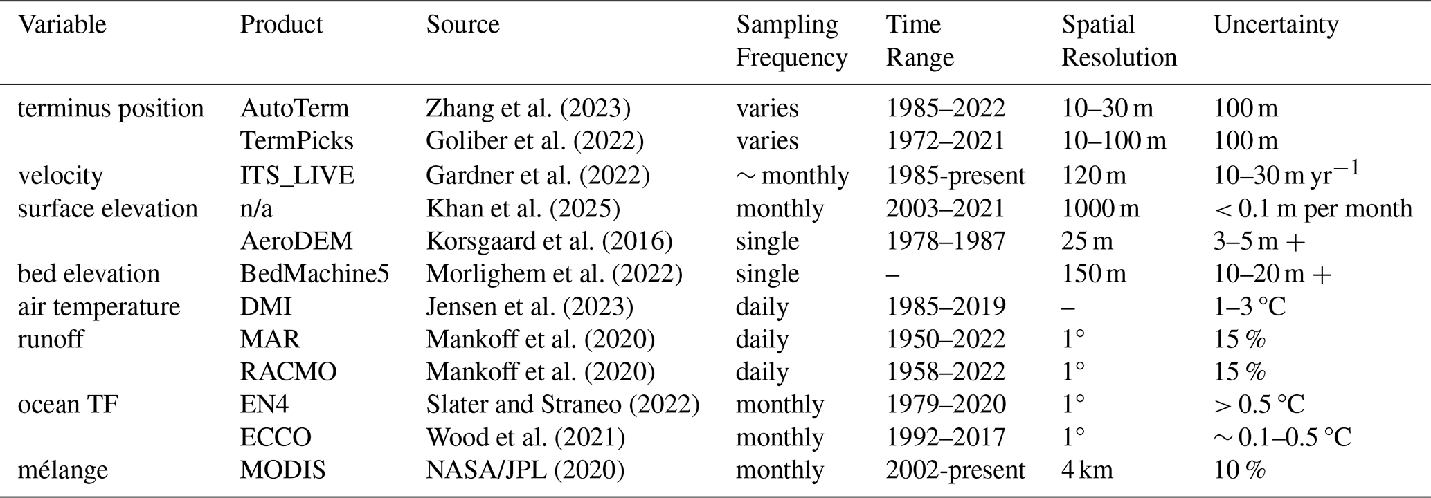
Because the drivers of seasonal terminus change are numerous and uncertain, we use data covering a wide range of observational variables suggested from the literature to have some control over terminus change (Table 1). We group these data into three categories that we term glacier dynamic data, climate data, and geometric data. Glacier dynamic data include glacier velocity and strain rates. Climate data include air temperature, ice sheet runoff, fjord mélange cover, and ocean thermal forcing. Glacier geometry data include surface elevation, bed elevation, ice thickness, and bed slope. Some of these data sets come from direct observations (e.g. air temperature) and some are model products (e.g. ocean thermal forcing). Where both direct observations and model products are available, we use the direct observation product to give our model a chance to learn patterns from the direct data. For some variables that are model products, multiple models produce similar products and we use several of these to run comparative experiments to determine whether one model product produces a more accurate forecast of terminus seasonality, while also considering the temporal coverage needed.

Zhang et al. (2023)Goliber et al. (2022)Gardner et al. (2022)Khan et al. (2025)Korsgaard et al. (2016)Morlighem et al. (2022)Jensen et al. (2023)Mankoff et al. (2020)Mankoff et al. (2020)Slater and Straneo (2022)Wood et al. (2021)NASA/JPL (2020)

Table 1 Publicly available data for Greenland glaciers used in our models. We extract these variables at the terminus for each glacier in Greenland.

Some data products are produced as time series (e.g., air temperature), but others (e.g., bed elevation) come as raster products that need to be converted into time series data. To produce a mean area value for these data sets, we clip the spatial extent of rasters near the terminus over an area bounded by the terminus position, fjord walls, and a line created from translating the map-view terminus position upstream (or downstream for products such as mélange) along a central flow line one stress-coupling length (Enderlin et al., 2016), here defined as 4-times the ice thickness, away from the terminus (Fig. 1). Because our terminus position changes with time, this bounding box thus moves with the terminus position in each time step creating Lagrangian time-series from raster data products.

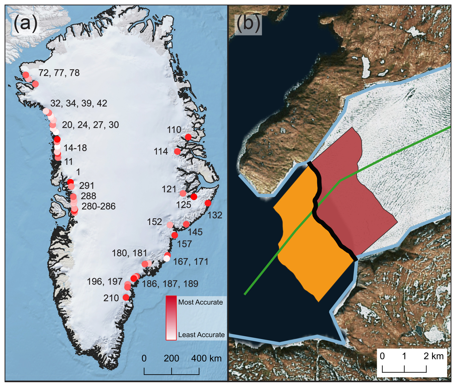
Figure 1 (a) Map of Greenland with locations of the 46 glaciers used in this study marked by circles and with GIDs labeled in black. Glaciers where the model created a more accurate prediction are in red with the least accurate models in white. (b) Sample of polygon generation for Store Gletscher (GID 284). The black line shows the terminus trace, the green line is the center flowline, and the light blue lines are the fjord walls. The red polygon generates upstream and is used to clip rasters of glacier data, such as ice flow velocity. The orange polygon generates downstream and is used to clip rasters of sea data, such as mélange. The thickness of both polygons is set to 4-times the ice thickness. Basemap for (a) accessed from Moon et al. (2023). (b) Sources: Esri, Maxar, Earthstar Geographics, and the GIS User Community | Powered by Esri.

2.1 Data Used

Glacier terminus data come from AutoTerm, a machine-learning pipeline designed to extract map-view terminus traces for Greenland (Zhang et al., 2023), and TermPicks, a database of manually traced terminus positions (Goliber et al., 2022). AutoTerm is chosen because it is the most complete terminus record for Greenland, with terminus picks from over 430 000 satellite images of Greenland between 1984–2021 (Table 1) and an increased temporal sampling to represent seasonality of terminus positions since the launch of Sentinel-1 in 2014. TermPicks is added to increase data density, particularly for earlier dates in some regions because data in TermPicks come from a wider range of satellite sensors. We compute terminus change using the center-line approach (Lea et al., 2014) using centerline shapefiles provided by Goliber et al. (2022). From this data, we also report the total terminus change from 2000–2020 as well as the mean of seasonal variation in terminus position over this time period for each glacier in Table 3.

Ice velocity data are obtained from ITS_LIVE image-pairs (Gardner et al., 2022) with less than 100 days separating the two images. We use ITS_LIVE for its high temporal and spatial resolution (Table 1). Strain rate data are derived from the gradients of ITS_LIVE image-pair velocities using finite differencing and represent the along-flow stretching rate (${\dot{\mathit{\epsilon }}}_{xx}$) where x is the along-flow direction. Monthly ice surface elevation data are from Khan et al. (2025), which provides data from January 2003 to August 2023 using a combination of radar altimetry data from CryoSat-2 and EnviSat, laser altimetry data from ICESat and ICESat-2, and laser altimetry data from NASA's Operation IceBridge Airborne Topographic Mapper. To extend temporal coverage of ice surface elevation time series, we include data from the AeroDEM flight mission from 1984–1985 (Korsgaard et al., 2016), which gives our time series a pre-2000 trend that is interpolated to begin in 2000. Bed elevation data come from BedMachineV5 (Morlighem et al., 2022), which is a modeled bed elevation based on mass-conservation principles. BedMachine has an uncertainty of ∼ 50 m for most of Greenland, with uncertainties possibly > 500 m close to termini of outlet glaciers where radar data are scarce. To avoid the high end of uncertainties, we exclude glaciers where the BedMachineV5 error scores are greater than two standard deviations above the mean for the 291 glaciers we have terminus data for (Zhang et al., 2023). Past studies found that bed elevation from BedMachine may be offset from existing radar data, but that bed slope is consistent with that found in radar (Catania et al., 2018). Surface and bed topographic data in combination are used to get ice thickness time series for each glacier.

Air temperature data for each glacier is assigned based on data from the most proximal of 26 Danish Meteorological Institute daily weather stations that have continual data starting in at least 2000 (Jensen et al., 2023), with distances between glacier and station ranging from 16.4 to 309.4 km (Supplement Table C1). For all stations used, station elevation was less than 100 m above sea level and so a lapse correction to account for elevation differences was not performed. Runoff data comes from Mankoff et al. (2020), which provides runoff estimates from two different regional climate models, the Regional Atmospheric Climate Model (RACMO) and the Modèle Atmosphérique Régional (MAR). For both products, Mankoff et al. (2020) calculates the liquid runoff occurring within a glacier catchment and assumes that all of that runoff routes to the glacier terminus. See Fig. 3 for a comparison of these two data sets for a single glacier. For an ocean climate proxy, we use ocean thermal forcing (OTF) – the difference between in-situ temperature and the salt- and pressure-dependent freezing point of seawater. As seasonal observations are not consistently available for most marine-terminating glacial fjords, we use modeled ocean temperature data from the continental shelf, which is processed as values depth-averaged in the lowest 60 % of the water column and resolved into glacial fjords from Wood et al. (2018). Two ocean thermal forcing products meet our temporal and spatial requirements; (1) Slater and Straneo (2022) used continental shelf ocean temperatures from the EN4.2.1 product from the United Kingdom's Met Office Hadley Centre (here called EN4; (Good et al., 2013)) and; (2) Wood et al. (2021) used continental shelf ocean temperatures from the Estimating the Circulation and Climate of the Ocean (ECCO) ocean state estimate (Fig. 3). These two models provide forcing at varying timespans and resolutions. ECCO has a 4 km spatial resolution but ends temporally in December 2017 while EN4 has a 1° resolution but extends through 2021 (Table 1).

While mélange has been demonstrated to have an impact on terminus calving rates, there is no consistently agreed-upon measure for mélange strength. Recent work suggests that calving dynamics may correlate with mélange thickness (Meng et al., 2025) and stiffness (using InSAR (King et al., 2021)), but there is no publicly-available long-term record of mélange strength or thickness for Greenland. We thus follow Cassotto et al. (2015), who used sea-surface temperature (SST) data from the Moderate Resolution Imaging Spectroradiometer (MODIS) to show that low (below zero) SST values in the Jakobshaven fjord correlate with seasonal advance of the glacier, likely due to mélange growth in winter. Thus, our metric for mélange is simply reflecting the presence or absence of mélange with the acknowledgment that we may be, at times, capturing other influences such as fjord ice. While this method is an imperfect proxy for mélange, SST provides a consistent, physical indicator of fjord ice conditions that influence terminus stability. Low SST values reflect the presence of ice-covered or near-freezing waters, conditions under which mélange forms and persists. By sampling SST directly in front of the terminus, we focus on the portion of the fjord most relevant to calving dynamics. Although SST does not capture all mélange mechanical properties, its seasonal variability has been shown to correlate with terminus position (Cassotto et al., 2015), supporting its continued use as a proxy for mélange presence. Thus, following Cassotto et al. (2015), for a mélange presence proxy we use MODIS Terra Level 3 SST data (NASA/JPL, 2020), which has monthly temporal resolution, 4 km spatial resolution, and a roughly 10 % uncertainty in cold waters. Because this product begins in 2002, two years after our start date, we artificially extend the MODIS time series back two years by duplicating the entire year of 2002 data for 2001 and 2000.

Data are prepared by interpolating each time series variable described above to daily values using approximation by localized penalized splines (ALPS), which has already been shown to perform well on time series of ice sheet thickness, elevation, velocity, and terminus locations (Shekhar et al., 2020). Interpolating data to a common temporal frequency allows us to link all input variables in a single data frame and smooths the data, removing extreme outliers (Fig. 2 and Supplement Fig. S1–9). In order to isolate the seasonal signal within our designated twenty year period, we separate the seasonal component from the multi-annual component for each input variable using a singular spectrum analysis (Elsner and Tsonis, 2013), which results in a zero mean over the time series and normalizes seasonal starting times, but not the magnitudes, of each data set (Fig. 2 and Supplement Fig. S1–9). The resulting time series are representations of each variable's seasonality, which we refer to simply as seasonality or seasonal magnitude for the remainder of the text.

It should be noted that the singular spectrum analysis does not completely prevent long-term trends from influencing seasonality, as some degree of interaction between these signals is expected and physically meaningful, reflecting a real coupling in the data. Indeed, Greene et al. (2024) found seasonal amplitudes of terminus change was the only variable in their study to strongly correlate with multi-decadal retreat. While isolating the seasonal signal focuses our analysis on intra-annual variability, we acknowledge and expect that multi-annual trends still exert some influence.

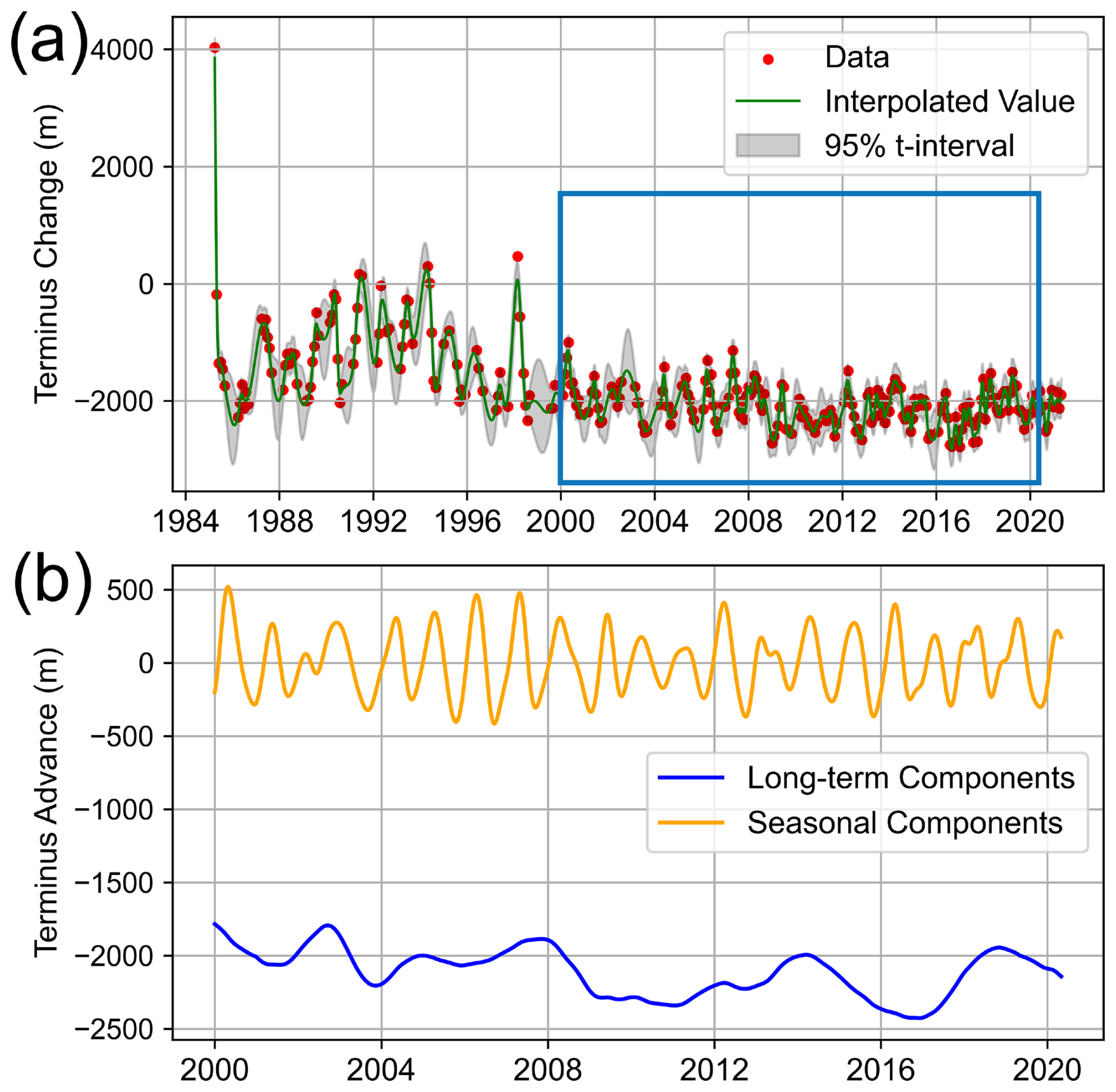
Figure 2 Sample data preparation for the terminus position change for Rink Isbræ (GID 1). (a) Approximation by localized penalized splines (ALPS) showing original data points in red, daily interpolation series in green, and the interpolation's 95 % confidence interval in gray. Data used from 2000–2020 boxed in blue. (b) Long-term and seasonal trend components separated from the time series by single spectrum analysis (SSA). The SSA was conducted only on data from 2000–2020.

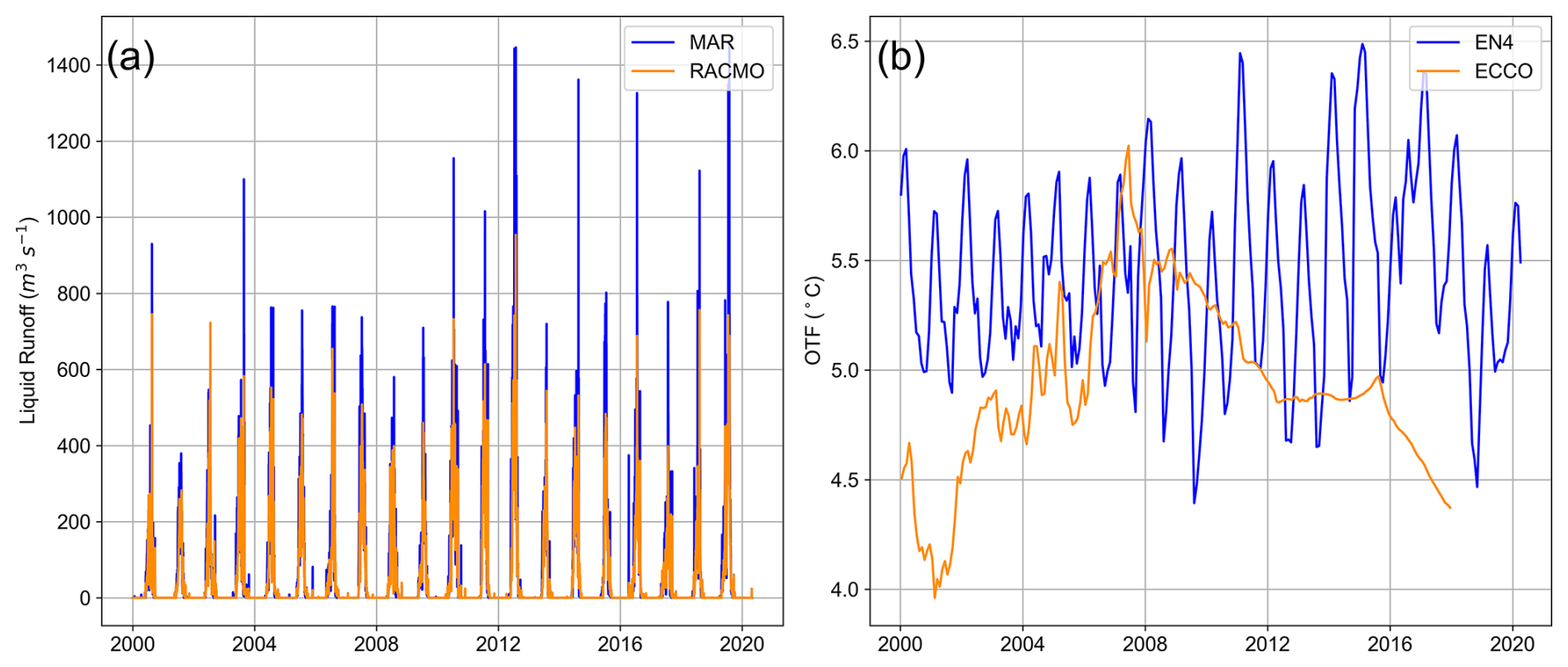
Figure 3 Comparative datasets from Rink Isbræ (GID 1) for (a) runoff and (b) ocean thermal forcing, from January 2000 to May 2020.

2.2 Glacier Selection

We begin by considering the 291 glaciers with terminus position time series from AutoTerm (Zhang et al., 2023). From these, we identify a subset of 115 glaciers that also have ocean thermal forcing data because Slater and Straneo (2022) limit their study to glaciers with a mean annual ice discharge greater than 2.5 m³ yr⁻¹. Of these 115 glaciers, we identify 46 glaciers with the most complete data coverage across all of our input parameters and within two standard deviations of reported uncertainties in bed elevation near the terminus (Morlighem et al., 2022). For these 46 glaciers, we produce characteristic data to understand the heterogeneity in this population (Table 3) using the same data sets described above and calculating averages over the period 2000–2020. We compute median annual velocities, mean grounding line depth, mean ice thickness, mean seasonal terminus change, and total terminus change (retreat is reported as a negative value). We also calculate the height above buoyancy for each glacier following Van der Veen (1996) as $H_{\mathrm{ab}}=H-({\mathit{\rho }}_{\mathrm{sw}}/{\mathit{\rho }}_{\mathrm{i}})D$ where H is the ice thickness, ρ_sw is the density of seawater, ρ_i the density of ice, and D is the grounding line depth. We compute the median H_ab for each glacier over the time period and define glaciers with a median H_ab value of ≤ 50 m as “near floating” and those with > 50 m H_ab as “grounded” following Van der Veen (1996) and Goliber et al. (2022). We also define a “mixed” status in which changes in flotation status occurred at least once between 2000–2020.

2.3 Machine-learning Analysis

We employ a machine learning regression time series analysis to predict and examine seasonal terminus change. We first create a model that most accurately forecasts the seasonality of each individual glacier and then probe the model to understand the importance of various input variables to model prediction. We run our regression forecasts using XGBoost, a computationally inexpensive Gradient Boosting decision tree method (Chen and Guestrin, 2016). XGBoost has a record of making accurate predictions from complex, multivariable relationships (Aydin and Ozturk, 2021) similar to those we expect to find in our study. While deep neural network-based approaches such as Long Short-Term Memory (LSTM) models are often applied in modeling time series data, they typically require very large data volumes to robustly train, may have trouble adapting to heterogeneous or missing data, and can be difficult to interpret (Hutson, 2018; Molnar, 2020; Stevens et al., 2020).

We set seasonal terminus position as our target model variable for forecasting and all remaining data are used as input features. We then divide the data into training and testing subsets using a temporal split, with the first 80 % of each time series being used to train our model and the final 20 % of each time series being used to test the model forecasting accuracy. No lag features are included in the input data. For our time period, this means we train our model using data from 1 January 2000 to 6 April 2016 and we test our model using data from 7 April 2016 to 1 May 2020. We then tune seven model hyperparameters (n_estimators, max_depth, learning_rate, alpha, reg_lambda, max_delta_step, colsample_bytree) using Bayesian Optimization (Bergstra et al., 2013) and set root mean squared error (RMSE) as the evaluation metric to reduce prediction error and improve model accuracy. We run an individual model for each of the 46 glaciers, with each glacier modeled only using data from that glacier. Further model setup details may be viewed at the link in the Code and data availability section.

Due to the iterative nature of decision tree models and XGBoost's internal feature tracking, we can track the impact and importance of each input variable through feature importance analysis, a concept inherited from economic applications of game theory. We use SHapley Additive exPlanations (SHAP), which tracks each step of our XGBoost model to compute and weigh the importance of each input variable on the produced time series prediction (Lundberg and Lee, 2017; Lundberg et al., 2018; Shapley, 1953). At every time step, SHAP assigns an importance value to each input variable based on its use in predicting the target variable, with the SHAP values of all input variables adding up to the predicted value (see for example Fig. 4c). Over the full test window of predicted values, we then add the absolute SHAP values for each input variable to determine their overall contribution, or importance, in our model's prediction. In addition to this, we create relationship plots between SHAP values and seasonal variations in each input variable to identify trends in the input variables that highlight how the variable exerts control on terminus position (e.g., linear or non-linear relationship, see for example Fig. 4d).

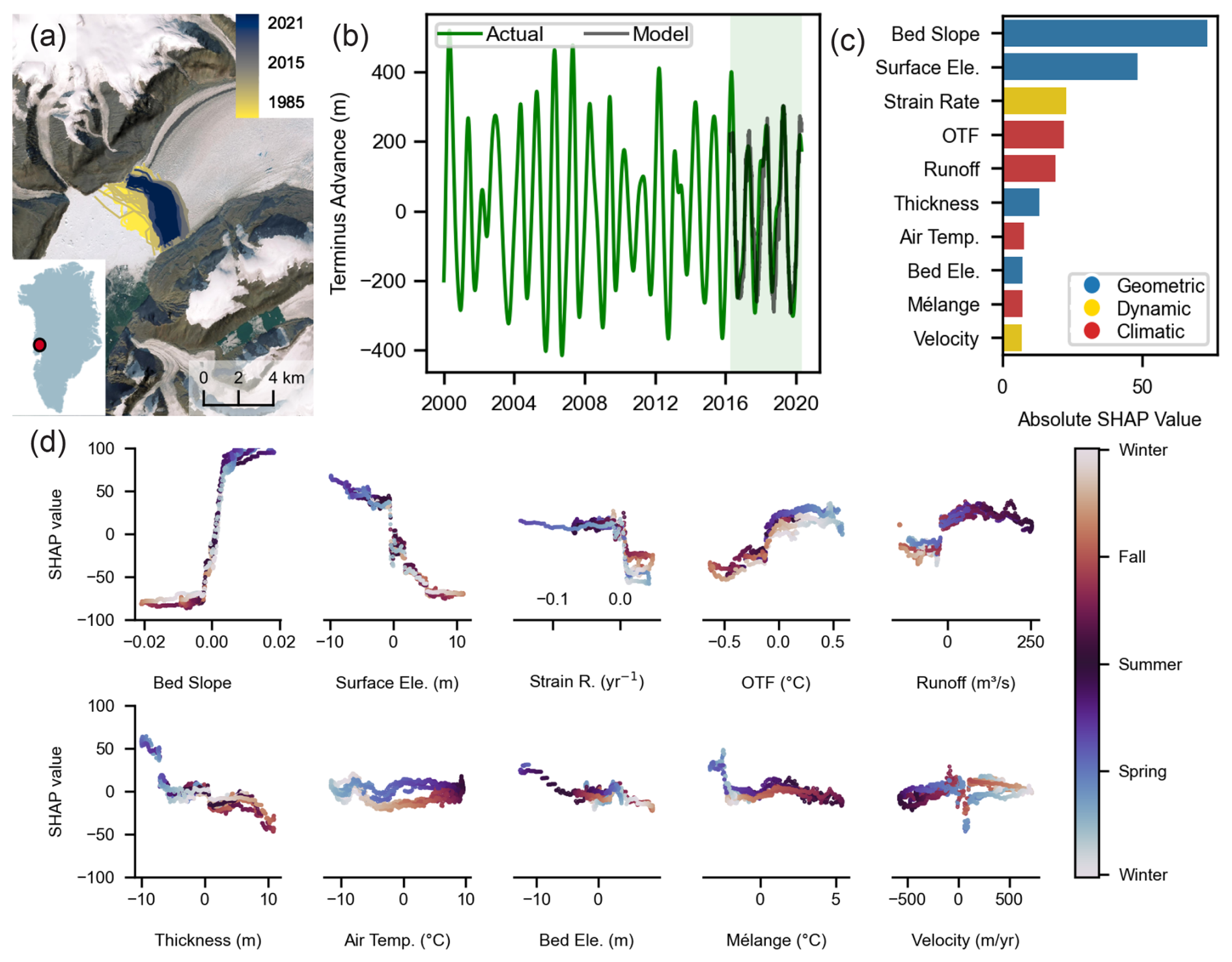
Figure 4 Model results for Rink Isbræ (GID 1). (a) Glacier location in Greenland and terminus traces colored by time. (b) Seasonal component of terminus change from 2000–2021 (green) with model prediction from Experiment 1 (black). (c) Absolute values of Shapley (SHAP) scores for each input variable, ranking variables by prediction importance. Variables are colored by variable group as indicated in the legend. (d) Relationship plots showing the variability of feature importance over a year. Data points are colored by time of year. Error scores for this model are NRMSE: 0.096 (RMSE: 90 m); Spearman: 0.885; R²: 0.783; offset: 2.5 weeks. Mélange referenced refers to sea surface temperature as a proxy for mélange presence. Sources: Esri, Maxar, Earthstar Geographics, and the GIS User Community | Powered by Esri.

2.4 Model Accuracy and Experimental Design

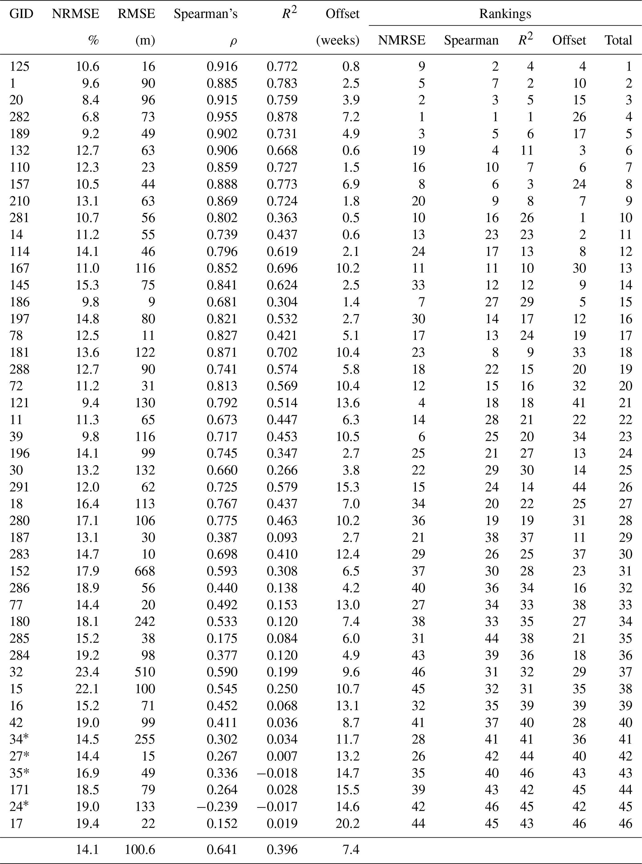
To examine the goodness of fit of our model results we examine three model statistics: the normalized root mean squared error (NRMSE), the Spearman (rank) correlation coefficient, and the coefficient of determination (Table 4). The NRMSE, here presented as a %, represents the root mean squared error normalized to the mean seasonal range of the target variable in order to compare model accuracy between glaciers of varying seasonal magnitudes. Lower NRMSE values generally indicate a better model fit, as it suggests that the model is making more accurate model predictions. Spearman's rank correlation coefficient (represented with a ρ) is a statistical measure of the strength and sign of a monotonic relationship (whether linear or not) between paired data. Correlations vary between −1 and +1, with 0 implying no correlation. Finally, we also examine the coefficient of determination, denoted as R², which gives a measure of how well observations are replicated by the model based on the proportion of the total variation of outcomes explained by the model. In addition to these statistical tests, we also examine the absolute difference in time, here called model offset, between peaks in the modeled and observed seasonal terminus position annually, including both the annual high and annual low points.. This gives a measure of the goodness of fit of the timing of changes in terminus position. For each glacier, we rank the value of each of our four model fit statistics and then produce a final weighted average ranking for all 46 glaciers that describes the overall goodness of fit (Table 4). We also provide the root mean squared error (RMSE) in meters as a direct measure of model accuracy (Table 4). It is important to note that we use NRMSE as the primary means of evaluating model accuracy, as the model is only trained to reduce RMSE, not other statistical measures.

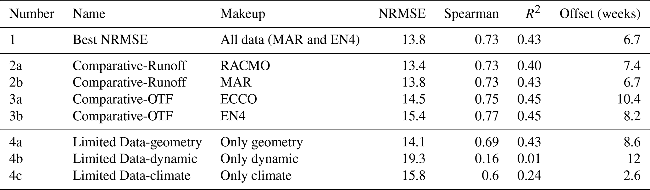
We run and report results on eight different experiments (Table 2). Our Best NRMSE Model (Experiment 1) represents the best-performing models for each glacier, using the full set of input datasets and using MAR for runoff and EN4 for ocean thermal forcing. We run two comparative experiments that examine the model fit when using different data products for runoff and ocean thermal forcing. Experiment 2 compares RACMO (model 2a) and MAR (model 2b) and Experiment 3 compares ECCO (model 3a) and EN4 (model 3b). For Experiments 3a and 3b, we shortened the model timespan from May 1st, 2020 to December 1st, 2017 due to the temporal limitation of ECCO. We also ran Experiment 3 on 8 fewer glaciers, as ECCO did not have data for these glaciers. Finally, we run three limited data experiments to understand the impact of data choice on model fit. First, we run the model using only geometric variables (Experiment 4a) including ice thickness, bed elevation, surface elevation, and bed slope. Second, we run the model using only dynamic variables (Experiment 4b) including ice velocity and strain rates. Third, we run a model using only climate variables (Experiment 4c) including mélange, ocean thermal forcing, runoff, and air temperature.

Table 2 List of experiments ran, their description, and model error scores. Error scores for Experiment 1 and 2b are the same because our Best NRMSE model uses MAR data. Experiments 3a and 3b are temporally shortened to the end of 2017 to account for ECCO temporal limitations.

3 Results

3.1 Glacier Characteristics

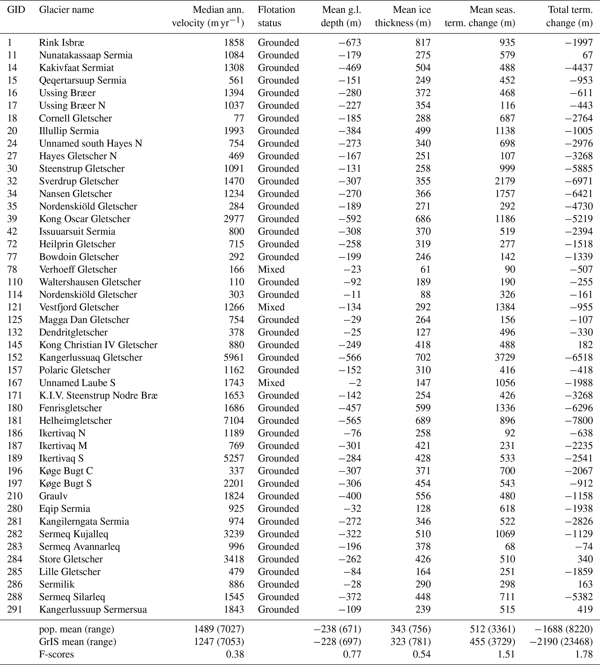
The population of glaciers used in this study represents just 16 % of the 291 glaciers in Greenland with terminus position data from Zhang et al. (2023). Geographically, our population of study glaciers excludes glaciers from the northern, southern, and southwestern coasts. We also exclude glaciers with large floating tongues (Fig. 1a). 89 % of the glaciers in our population underwent long-term retreat over the observational time period with an average total retreat of 1.7 km (range of 8.2 km; Table 3). 93 % of the glaciers in our population are grounded over the observational time period with a mean grounding line depth of 238 m (range of 671 m) and mean ice thickness of 343 m (range of 756 m). Finally, the population of glaciers we examine have a median terminus velocity of 1.49 km yr⁻¹ (range of 7.03 km yr⁻¹) and exhibit seasonal amplitude changes of 512 m (range of 3361 m). When comparing our population of glaciers to the total Greenland-wide population, we find that our population is slightly faster, deeper, thicker, and experiences larger seasonal changes in terminus position but has less total terminus change over the observation period (Table 3). We also performed ANOVA-F tests (Fischer, 1925) to assess whether individual glacier characteristics (velocity, grounding line depth, ice thickness, seasonal terminus change magnitude, and long-term terminus change) are associated with the top-ranked feature importance. We report these F-scores at the bottom of Table 3 and find a moderate correlation between our glaciers' retreat history, both seasonal and long-term, and their feature importance. We find a weak correlation between the other characteristics and feature importance.

Table 3 Glacier characteristics for the 46 glaciers chosen in this study. Data are averaged annual values over the period from 2000–2020. See text for description of flotation status and F-scores. At the table's end are mean values for the 46 study glaciers (pop. mean) and for 269 glaciers (terminus data) and 113 glaciers (geometric and velocity data) with data in Greenland (GrIS mean), with range of values shown in parentheses.

3.2 Best NRMSE Model Experiments

For all 46 glaciers, we forecast terminus changes during the test period (2016–2020), achieving mean model statistics of 13.8 % NRMSE, 0.73 for Spearman's ρ, a mean R² of 0.43, a mean offset of 6.7 weeks, and a mean RMSE of 100.6 m (Table 4). We use MAR for our runoff values and EN4 for the ocean thermal forcing values in our Best NRMSE Model because of the outcomes from our comparative experiments (described in detail below). For each glacier, we plot its location in Greenland with the change in terminus position over the study period, the seasonal variability in the terminus position with our model prediction, the SHAP analysis, and a set of relationship plots that examine how the importance of individual features vary over a year (see example Fig. 4 and Supplement). In addition to inspecting model fit statistics, we use these figures to visually inspect our model predictions to determine the success of our models. From visual inspection, we find four failed forecasts with model predictions not showing any seasonal terminus change (GIDs 24, 27, 34, 35; Fig. 5a). These four glaciers have high NRMSE scores and rank low overall in our total statistical ranking (Table 4). Most of these failed predictions have poorly resolved seasonal terminus change as input data, which may have been a consequence of using the Singular Spectrum Analysis to isolate the seasonal signal from the long-term signal.

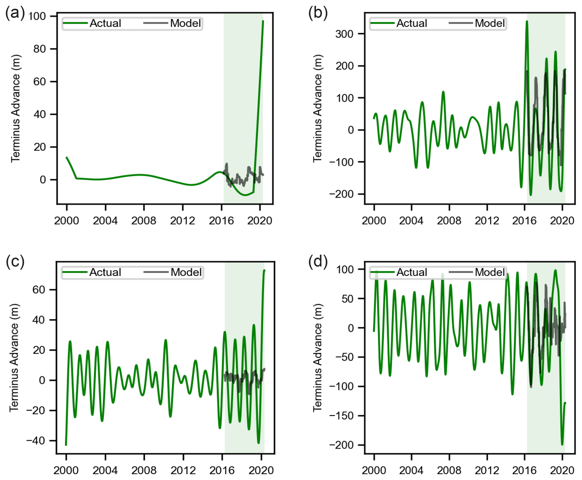
Figure 5 Additional prediction plot samples, showing the seasonal component of terminus change from 2000–2021 (green) with model prediction from Experiment 1 (black). (a) GID 27: forecast does not show any seasonal terminus change. (b) GID 197: forecast underestimates the full seasonal amplitude. (c) GID 17: forecast greatly underestimates seasonal magnitude. (d) GID 286: glacier exhibits erratic seasonality.

In addition to four failed models, we find a range in success of our machine-learning model to predict seasonal change (Supplement and Table 4). We divide the glaciers into two halves using Table 4 and compare the top half of our ranked glacier model statistics (up to rank #23) to the bottom half. The top half of the models have a mean NRMSE of 11.3 %, mean Spearman's ρ of 0.829, a mean R² of 0.612, and a mean offset of 4.9 weeks. Comparatively, the bottom half of the models have a mean NRMSE of 16.8 %, mean Spearman's ρ of 0.454, a mean R² of 0.179, and a mean offset of 9.9 weeks. Comparing top- to bottom-ranked models, we find that more accurate seasonal terminus position predictions come from glaciers that are faster (883 m yr⁻¹ vs. 723 m yr⁻¹), with deeper grounding lines (258 m vs. 199 m), larger seasonal terminus variations (522 m vs. 510 m), and have experienced less long-term retreat over the 20-year time period of our study (1005 m of retreat vs. 2234 m of retreat). We find little variation between these two groups regarding ice thicknesses (346 m vs. 340 m). While many top-predicting models closely approximate observations, some underestimate the full seasonal amplitude of terminus change (GIDs 78, 132, 197; Fig. 5b). Among the poorly performing predictions, we see models that either greatly underestimate seasonal magnitudes (GIDs 16, 17, 284; Fig. 5c), exhibit no seasonality (GIDs 24, 27, 34, 35; Fig. 5a), or have erratic seasonal signals (GIDs 284, 285, 286; Fig. 5d).

Table 4 Glacier model statistics for all 46 glaciers chosen for this study. Glaciers are arranged according to their total model weighted rank, which is a simple average of NRMSE, Spearman's ρ, R², and offset. Bottom row of bolded values represents the mean statistics for the population. Four models fail to produce seasonal changes in terminus position are marked with an asterisk.

Among all modeled glaciers, we identify the variable group most relied upon for predicting seasonal terminus change from the SHAP feature importance analysis and find that the majority of glaciers (74 %) have geometric variables as the most important variable group compared to 13 % for dynamic variables and 13 % for climate variables (Fig. 6a). Among our top half of ranked glaciers, the number of glaciers that rely on geometric and climatic variables increases (78 % and 17 % respectively) while reliance on dynamic variables decreases (4 %). Meanwhile, among our bottom half of ranked glaciers, reliance on geometric and climatic variables decreases to 70 % and 9 % of this population while reliance on dynamic variables increases to 22 %. Considering variables individually among all modeled glaciers, we find bed slope to be the most frequent top predictive variable while air temperature was the least predictive variable for any glacier (Fig. 6b). However, our model results suggest that terminus change is not a simple function of a single variable. Instead, we find that model prediction relies on multiple input variables to create its forecast, with the majority of glaciers needing on average five input variables to explain 75 % of the terminus change observed (Fig. 7).

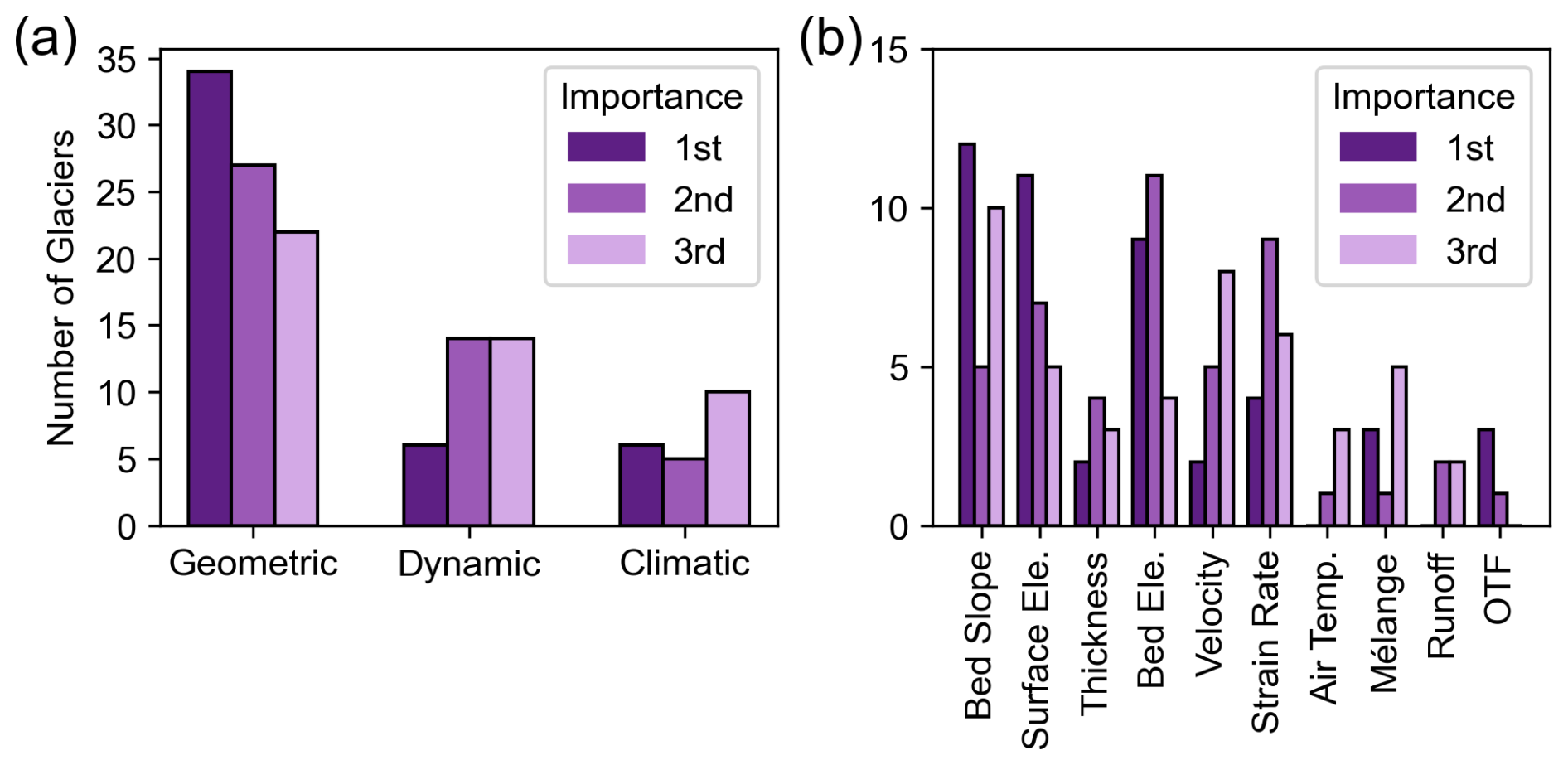
Figure 6 (a) Shapley value (SHAP) feature importance for all 46 glaciers in the Best NRMSE Experiment (Experiment 1), Results show whether the three most important input variables for model prediction were geometric (bed elevation, bed slope, ice thickness, or surface elevation), dynamic (ice flow velocity or strain rate), or climatic (air temperature, runoff, ocean thermal forcing, or mélange). (b) Same results, but showing individual variables and their feature importance.

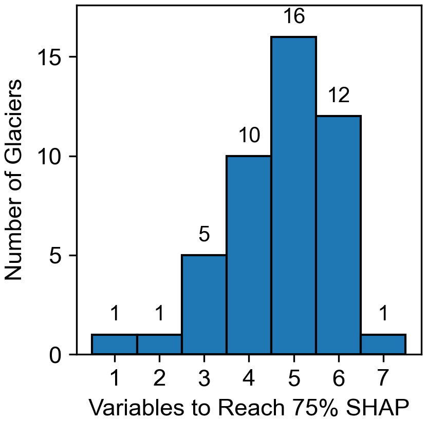
Figure 7 Histogram of the number of input variables needed to define 75 % of the SHapley Additive exPlanations (SHAP) value score for the Experiment 1 model prediction for all 46 glaciers. Numbers on top of each bar indicate the number of glaciers in the bin.

To better understand the relationship between the seasonal values of input variables and their coinciding SHAP values, we examine the relationship plots for each glacier (Fig. 4d and Supplement). By inspecting these relationship plots, we can see when in the seasonal cycle an input variable gains importance and how input variable values correlate to SHAP values. For our example glacier (Rink Isbræ), we find terminus advance (high positive SHAP value) for positive bed slopes in late Spring through to the beginning of Summer and terminus retreat (high negative SHAP value) for reverse bed slopes in Fall. For surface elevation, we find an opposing trend, with thinning associated with advance (high positive SHAP value) in Spring/Winter and thickening associated with retreat (high negative SHAP value) in Summer/Fall. Variables with less importance to predicting the terminus position (e.g. bed elevation, mélange, and velocity for Rink Isbræ in Fig. 4d) exhibit a flat trend as SHAP values hover around zero but we can still discern seasonal distributions of the variable values.

3.3 Comparative Experiments

We performed experiments to determine the change in model statistics when using different products for both runoff and ocean thermal forcing data. Experiment 2 focuses on comparing runoff products from RACMO and MAR. For this experiment, we find that the modeled seasonal terminus is relatively insensitive to the choice of runoff model. We obtain NRMSE scores of 13.4 % for RACMO and 13.8 % for MAR (Table 2), with 20 glaciers exhibiting lower NRMSE using RACMO and 26 glaciers when modeled with MAR. The NRMSE scores vary by up to 3.8 % between MAR and RACMO. We find similar small differences in the Spearman, R², and offset statistics. We ultimately chose to run our Best NRMSE models (Experiment 1) using MAR because it reduced the modeled temporal offset of seasonal change to 6.7 weeks instead of 7.4 weeks for RACMO (Table 2).

For Experiment 3, we compare the different ocean thermal forcing products from EN4 and ECCO. For this experiment we had to reduce total model time by 2.5 years because ECCO data is only available until 2017. Thus, we first re-run our model Experiment 1 (Best NRMSE Model result) shortened to 2017 and get a new Best NRMSE Model result using this shortened time period. This model uses EN4 and produces a NRMSE of 15.4 % and a temporal offset of 8.2 weeks (Table 2), representing an overall increase in the NRMSE from 13.8 % and an increase in offset from 6.7 weeks. We then run our model swapping in ECCO data for ocean thermal forcing and find a model NRMSE of 14.5 % and a temporal offset of 10.4 weeks. Thus, the ECCO model produces a more accurate modeled fit to the seasonal terminus change observations (in terms of NRMSE) but there is an increased lag time between modeled terminus change and observations of roughly two weeks. Despite the improved model NRMSE when using ECCO, we use EN4 for our Best NMRSE Model results because the time span of data availability allows for overall reduced NMRSE.

3.4 Limited Data Experiments

To evaluate the importance of grouped geometric, dynamic, and climatic data on our model results, we conduct experiments using only variables from each one of these groups. These tests aim to determine changes in model accuracy that provide insight into the model variables that best predict seasonal terminus change. Because these experiments involve a reduction in training variables when compared to our Best NRMSE Model, we expect less accurate forecasts, particularly for those model runs where we exclude variables with high importance. Conversely, we expect minimal change in accuracy when we remove less important variables.

Experiment 4a are geometry-only models in which we only include geometric variables (surface elevation, bed elevation, ice thickness, and bed slope). These models perform the best of the limited data experiments, with an NRMSE of 14.1 %, which is just a 0.3 % increase over the Best NRMSE Models. Experiment 4b, the dynamic-only models (only including strain rate and velocity data), are the worst-performing models with an increase in NRMSE to 19.3 %, representing a 5.5 % increase over the Best NRMSE Model. Finally, in Experiment 4c, the climate-only models (including only mélange presence, runoff, air temperature, and ocean thermal forcing), have an average NRMSE of 15.8 %, representing an increase of 2.0 % over the Best Fit Model. Similarly, both the Spearman and R² values are highest for the geometry-only models and lowest for the dynamic-only models. Of particular interest, while our Best NRMSE Models have a mean temporal offset of 6.7 weeks, we see increases in temporal offset in both the geometry-only and dynamic-only models, but a large reduction to 2.6 weeks in temporal offset in our climate-only models. This is likely because XGBoost trains with an iterative goal of reducing the model RMSE, so our Best NRMSE Models (Experiment 1) reduce the model RMSE but likely at the cost of a more accurate offset. Model results for Experiment 3c, simplified to only training on climate data, do not capture total seasonal amplitudes (thus have higher error scores), but perform the best at reducing the seasonal offset. The poor model results for Experiment 4c, the dynamic-only models, may be the result of too little training data, as they use only two variables compared to four variables in the geometry-only and climate-only models.

4 Discussion

4.1 Feature Importance for Magnitude of Seasonal Terminus Prediction

Our results indicate that the geometry of the near-terminus region (bed elevation, bed slope, ice thickness, surface elevation) is the most important predictor of seasonal terminus change, with bed slope being the most important individual predictor (Fig. 6). Past authors have also suggested a correlation between local glacier geometry and changes in terminus position (Bassis and Jacobs, 2013; Catania et al., 2018; Enderlin et al., 2013; Frank et al., 2022; Schild and Hamilton, 2013; Vieli and Nick, 2011). This connection is logical because topography at the terminus controls the driving stress and thus velocity of ice moving towards the terminus. Topography also controls the ability of a glacier to reach flotation, which promotes calving (Amundson et al., 2010; James et al., 2014). Indeed, Bassis and Jacobs (2013) found, using a different approach, that ice thickness and bed geometry are first-order controls on calving. The model reliance on bed slope is also consistent with the idea that termini cannot be stable on reverse bed slopes (Schoof, 2007) because glaciers are more likely to calve when they retreat into deeper waters, such as overdeepenings that often exist right behind many glacier termini (Catania et al., 2018; Kehrl et al., 2017). Our results must be interpreted within the context of the model goal to reproduce the seasonal magnitude of terminus change, not its timing (i.e. the model is trying to minimize RMSE, not temporal offset). Indeed, timing of seasonal terminus change is best modeled when we use only climate data in our model (Experiment 4c), although this reduces model accuracy in predicting the magnitude of terminus change. Together, these results suggest that climate variables are important controls on the timing of terminus advance and retreat but that the total magnitude of terminus advance and retreat is controlled by geometry as has been found for a smaller number of glaciers by previous authors (Catania et al., 2018).

Extending beyond the predominant predictor of geometry, we can examine individual glaciers within our 23 top-ranked models where authors have identified seasonal or long-term drivers to terminus change. One such glacier is the well-studied Helheimgletscher (GID 181, Table 3), where our model predicts mélange to be the dominant predictor (predicting 17 % of the total terminus change). This agrees with Meng et al. (2025), who found thick mélange at the Helheimgletscher terminus correlates to seasonal calving, typical for glaciers with long fjord systems that trap mélange, enabling enhanced buttressing on the terminus as mélange thickness grows. Another study of Helheimgletscher (Ultee et al., 2022) found a strong correlation between runoff and seasonal terminus change. While our model found runoff only responsible for 9 % of the total terminus change (Supplement Fig. S39), Ultee et al. (2022) notably did not test for mélange. Our model also finds a high degree of importance for surface elevation (also 12 %), which agrees with the Ultee et al. (2022) observation that upstream surface thinning correlates to Helheimgletscher's retreat, and Kehrl et al. (2017), who found variations in surface thinning and bed geometry a few kilometers away from Helheimgletscher's terminus were responsible for the glacier's stable grounding line from 2008 to 2016.

In Central West Greenland, Fried et al. (2018) correlated seasonal terminus change from 2013–2016 to changes in mélange for Rink Isbræ, Sermeq Silarleq, and Store Gletscher (GIDs 1, 288, 284). Howat et al. (2010) found similar results from 2000–2009 for eleven glaciers in the same region, finding a strong correlation between the timing of mélange and the onset of retreat. Our model, which is trained to predict the magnitude of seasonal retreat, produced results for Rink Isbræ that do not place high importance on mélange, but find a top three importance for strain rate, indicating that the model may have translated the buttressing impact of mélange on the terminus to an impact on strain rate. Our estimate of mélange as the presence of low SST values in front of the terminus may misrepresent mélange strength, which may be more related to mélange thickness or rigidity. Our model result for Store Gletscher shows a high feature importance for mélange in agreement with Meng et al. (2025) and Fried et al. (2018), while our result for Sermeq Silarleq does not find a correlation with mélange at all. Unlike Store Gletscher and Rink Isbrae, Sermeq Silarleq experienced a long-term retreat and in ∼ 2013 the terminus of this glacier was retreating through an overdeepening and the glacier became more lightly grounded (Goliber and Catania, 2024). Glaciers that are closer to flotation are more sensitive to mélange conditions (Fried et al., 2018; Walter et al., 2012), however the training window for our model included data before, during, and after the retreat which may have diluted its ability to identify mélange as a highly important variable for Sermeq Silarleq. Seven other glaciers examined by Fried et al. (2018) overlap with our study including Eqip Sermia, Kangilerngata Sermia, Sermeq Kujalleq, Sermeq Avannarleq, Lille Gletscher, Sermilik, and Kangerlussuup Sermersua (GIDs 280, 281, 282, 283, 285, 286, 291). For these glaciers, Fried et al. (2018) found that changes in runoff correlate to changes in terminus position. We find mixed results. For many of these glaciers our models performed poorly (GIDs 280, 283, 285, 286) while for the remaining glaciers we only see runoff as an important variable for GID 281.

4.2 Complexity of Terminus Parameterization

Due to the heterogeneity in both feature importance (Fig. 6b) and number of variables needed to produce at least 75 % of the predicted terminus change (Fig. 7), we caution against a simple parameterization for seasonal terminus change. This heterogeneity in results may relate to complexities found in calving styles in Greenland (Bézu and Bartholomaus, 2024; Goliber and Catania, 2024) driven by three processes: undercutting driven by discharge or melt leading to serac failure (Benn et al., 2007), bending of glacier termini near-flotation leading to buoyant flexure (Amundson et al., 2010), and tensile rifting of glaciers with large ice tongues (Alley et al., 2023), which our study excludes. Prior studies have demonstrated that glacier calving style can change from one dominant style to another during retreat when glaciers enter overdeepened parts of their fjords (Bézu and Bartholomaus, 2024; Goliber and Catania, 2024), which further complicates seasonal terminus predictions.

Results from our best 23 performing glacier models, when compared to our general glacier population, suggest that improved model fit is biased towards glaciers with greater seasonal variations in velocity, grounding line depth, and terminus position. For example, our model for Rink Isbræ (GID 1), which has a mean seasonal terminus change of 935 m, outperforms glaciers like Sermeq Avannarleq (GID 283) whose terminus moves less than 100 m annually (Table 3). We find no correlation between model accuracy and seasonal changes to ice thickness (Table 3). Other authors have shown a clear connection between glaciers with large seasonal changes to terminus position and seasonal changes to velocity (Moon et al., 2014) and runoff (King et al., 2018). These large seasonal changes create data with high signal-to-noise ratios compared to their uncertainties, providing higher accuracy data for our models to train on and thus produce more accurate model results. The lack of correlation between high seasonal melt discharge and seasonal changes to ice thickness agrees with Moon et al. (2014), who found sub-annual changes to ice thickness reduced runoff seasonal amplitude.

We also find our best predictive models occur for those glaciers that are close to a steady state, having experienced less overall retreat during the 20 years of our study (Table 3). When glaciers do retreat, we notice a corresponding instability in their seasonality as they experience greater variations in bed geometries and flotation status. These results suggest that large amplitude seasonal signals may be the result of retreat through overdeepenings, not the cause of retreat as proposed by Greene et al. (2024).

4.3 Limitations of this Study

While we provide a new way to parameterize seasonal glacier terminus change, our machine learning approach comes with inherent limitations as to what our models can do and how their results can or should be interpreted. Limitations can be grouped into; (1) shortcomings inherent with decision tree models and; (2) shortcomings related to imperfect data. First, we will discuss data limitations. The data products used in our models are heterogeneous in terms of their quality and robustness for accurately representing the variable we aim to include. For example, many glaciers do not have radar-based ice thickness/bed elevation observations near their termini and we rely on an estimated product from BedMachine. While this product has demonstrated accuracy with representing the overall shape of the bed topography (Morlighem et al., 2022), there can often be offsets of up to a few hundred meters in elevation (Catania et al., 2018). In addition, there currently are no ice sheet-wide accurate measures of mélange strength and our choice of mélange presence (Cassotto et al., 2015) may not reflect the true impact of mélange on the terminus position for some glaciers (King et al., 2021; Meng et al., 2025). Our methods also require data with high spatial and temporal resolution covering glaciers with enough fidelity for at least 20 years, which limits our ability to include data products that are expected to influence terminus changes. This exclusion includes direct observations of freshwater flux (Karlsson et al., 2023), and observations of sedimentation at the terminus, which is expected to have an impact on bed geometry and terminus stability for some glaciers (Brinkerhoff et al., 2017).

Other issues arise from the need for multiple data preparation steps, including detrending seasonal components and interpolating daily values. While interpolating all data to daily values provides the quantity of data needed for our model, this process produces time-series with an artificially high temporal frequency compared to the original input data set, which is not real. Interpolation to daily values may ultimately hide trends in data that influence the terminus. Also, our use of ALPS for interpolation (Shekhar et al., 2020) introduces a level of error as the interpolation on occasion interprets noisy seasonal data poorly, sometimes removing seasonal changes. This failed interpolation can be seen in the terminus position data from Hayes Gletscher N (GID 27; Fig. 5a) and Nordenskiold Gletscher (GID 35; see Supplement), both of which failed to produce modeled seasonal terminus change. Further, the interpolation method used does not recognize seasonality equally across time series where data density improves with time. This is seen in the time series of strain rate and velocity produced from ITS_LIVE (Supplement Figs. S7 and S9), where the addition of Sentinel data increases seasonality in the time series after 2015 (Gardner et al., 2022). This potentially weakens the importance of these features in our results.

In addition to limitations associated with bad data and preparation, our results suffer from the choice of model. Every available machine learning model, such as the XGBoost algorithm that we employ, comes with built-in model weaknesses. One common weakness of many machine learning regression models is that they struggle to predict time series maxima with larger magnitudes than the range of data they are trained on (Breiman et al., 2017; Tan et al., 2022). We see this in our prediction results for many glaciers that have experienced long-term retreat, which often enhances the amplitude of seasonal terminus change as termini retreat through bed overdeepenings. If long-term retreat is constricted to the last part of the time series, falling outside our training data period, then the model is poorly trained and unlikely to predict seasonal disparities introduced from long-term retreat. For example, our model for Dendritgletscher successfully approximates seasonal magnitudes learned in the training data but cannot predict magnitudes in the testing data that exceed the magnitudes the model trained on (GID 132; see Supplement).

A challenge in interpreting the feature importance results in our methods is displayed by the high feature importance of strain rate along with the low importance of velocity in our Helheimgletscher result (GID 181; see Supplement). The model treats input variables in isolation while physically many variables are interconnected (James et al., 2013, also see Fig. 8). As a result, the model may rely on one predictive variable while overlooking another that is physically relevant but statistically redundant, leading to unstable results (Salih et al., 2025).

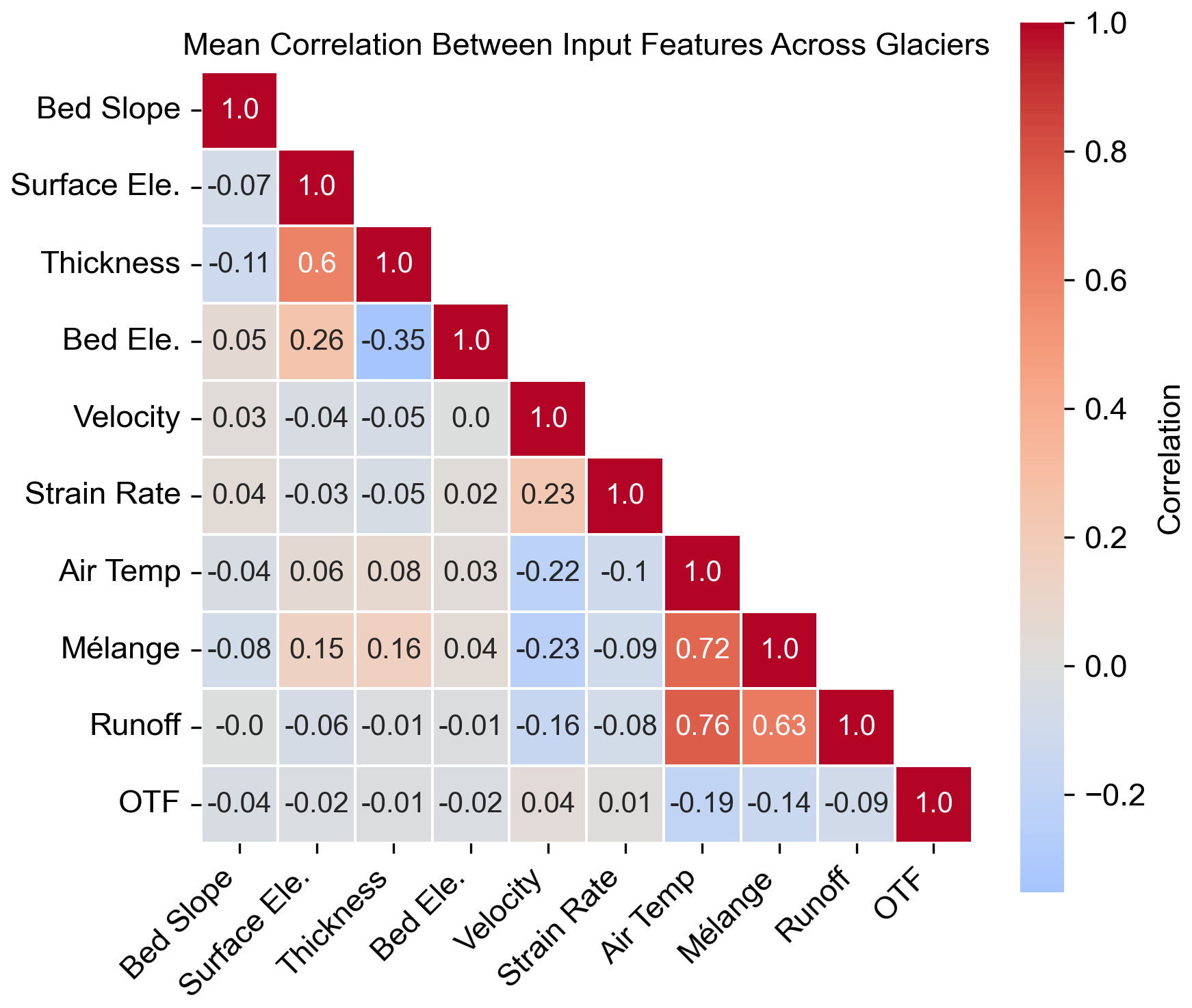
Figure 8 Heatmap of the mean correlation between input variables across all 46 glaciers used in this study.

4.4 Outlook

Despite these shortcomings, our model accuracy for a large number of glaciers highlights the potential for using decision tree models for improving our physical understanding of seasonal terminus position change and the use of machine learning in ice sheet modeling of terminus change. Using an additive decision tree algorithm instead of more complex machine learning options enabled us to use feature importance analysis to interpret the physical variables that drive seasonal terminus position change within each glacier system. Our methods are easily adaptable, allowing them to be applied to outlet glacier systems wherever data are available and reliable, and can be updated as new data are published.

Despite the complex interplay between fjord geometry, mélange buttressing, and oceanic and atmospheric forcing that occurs at glacier termini, our results highlight the predictive value of geometric variables alone on seasonal terminus position. This builds on the conclusions from previous studies demonstrating the importance of geometry in limiting glacier retreat (Catania et al., 2018; Meier and Post, 1987; Pfeffer, 2007) and those who find sediment deposition in front of a tidewater glacier facilitates glacier advance by decreasing water depth and reducing calving flux (Brinkerhoff et al., 2017; Nick and Oerlemans, 2006). Further, fjord geometry modulates how the ocean climate reaches termini with some moraines restricting the inflow of warm, saline Atlantic water, which has been linked to widespread terminus retreat (Carroll et al., 2018; Murray et al., 2010; Straneo and Heimbach, 2013). However, seasonal cycles in terminus position arise from the annual modulation of external changes in air temperature and ocean thermal forcing, making climate variables necessary for predicting terminus change accurately. These conclusions suggest that climate controls if a glacier retreats or advances, but fjord geometry dictates how much retreat or advance can occur. Such a complex interplay between climate and fjord geometry may explain the uneven response of glacier termini to external forcing, confirmed by Fischer and Aschwanden (2024), who found that Greenland glaciers occupy different stages of the tidewater glacier cycle. Our results confirm this complexity. Even on a seasonal timescale, terminus change is most accurately predicted when many variables are included, underscoring the necessity of including such complexity in predictive ice sheet models.

Complementary to improving physical process understanding, our decision tree model can be implemented within numerical ice flow models to provide improved glacial terminus position forecasting. An advantage our method has over traditional physics-based forecasting parameterizations is that it does not rely on one tunable parameter that must vary greatly between glaciers as it incorporates all sources of error into a single term (Morlighem et al., 2019). Incorporating decision tree models into numerical models can be an important advance in simulating complex, heterogeneous glacial systems where there is currently an incomplete understanding of the physics that govern glacier terminus position change. Future work focused on expanding our approach to long-term terminus position changes would make our modeling approach a strong candidate for integration into larger ice sheet modeling efforts, such as the Ice Sheet Model Intercomparison Project for CMIP7 (ISMIP7).

5 Conclusions

This study uses publicly available datasets for Greenland outlet glaciers that include geometry variables (ice thickness, bed slope, bed and surface elevation) ice dynamic variables (ice velocity and along-flow strain rate) and climate variables (ocean thermal forcing, runoff, air temperature, and mélange presence) into a machine learning model to predict outlet glacier terminus seasonality for 46 outlet glaciers in Greenland. We test model accuracy and find accurate predictions for roughly half of our glacier population that are characterized as deep, fast-flowing glaciers with large seasonal signals. Inspection of model results via the SHAP analysis shows that geometric properties (bed elevation and slope, surface elevation, ice thickness) are most relied upon for accurate predictions of our top-ranked models. We then perform a set of experiments to test for the predictive capacity of models with isolated input data (either geometry, climate, or dynamics in isolation) and find that geometric variables exert strong control on predictions overall, particularly in matching seasonal magnitudes, while climate data appears to have more control over predicting the timing of seasonal changes in terminus position. We also find that increased accuracy results when at least five variables are included suggesting that terminus parameterization is complex and potentially heterogeneous.

Our results shed light on the potential for machine learning to provide a mechanism for forecasting terminus change that could ultimately be incorporated into numerical ice sheet models that are physics-based. To improve on our results, more accurate data are needed, particularly for bed elevation (which is poorly resolved particularly at the termini of most outlet glaciers) and mélange strength. From the modeling side, as newer machine learning techniques evolve, other predictive algorithms should be considered for improved modeling accuracy. Higher model accuracy should, however, be carefully weighed if it comes at the cost of less interpretable results.

Further insight into additional processes that influence the terminus position not examined here (e.g. sedimentation at grounding lines) could also be an important missing part of our parameterization. Our approach relies on the consistent and sustained efforts of the scientific community to monitor change in the polar regions and to make those observations publicly available. This includes data from a range of platforms: ship-based (e.g., ocean thermal forcing), airborne (e.g., Operation IceBridge surface elevation), ground-based (e.g., runoff estimates from observation-constrained models), and satellite-based (e.g., terminus position and ice velocity). Without sustained funding for these critical observations, we risk losing our ability to predict changes in the polar regions and to deepen our understanding of the timing and magnitude of future Arctic change and global sea level rise.