A remote sensing approach for measuring climatic change effects on snow cover dynamics

Climate change (CC) is significantly impacting the snow cover of the European Alps, compromising hydrological cycles, water stock for agricultural and civil supply, winter tourism. This study investigates Snow Cover Changes (SCC) in the Western Italian Alps (Piemonte and Valle d'Aosta regions) from 2000 to 2023, using MODIS satellite data. In particular, MOD10A1 images were processed in Google Earth Engine to derive daily snow cover, integral snow cover area (iSCA), snow persistence (SP), and mean daily snowed area (MDSA). Ground data from 96 snowmeter stations were used to validate the satellite-derived SP. The analysis of SCC was performed by quantifying long-term trends of MDSA at the pixel level. The normalized trend (nT) index represents the percentage change rate in snow-covered area per yearly mean snow event. It was mapped showing different spatial patterns of SCC in the study area. Results reveal an altitudinal gradient in nT, with the higher snow cover reduction occurring in lowland and within main valley areas, reaching −5 % below 1000 m a.s.l. and −1.8 % between 1000–1500 m a.s.l. These findings highlight the vulnerability of snow resources due to CC, impacting water availability, winter sports, and regional economies. This study can support adaptation strategies and sustainable resource management in the Western Alps by mapping critical areas where CC effects on snow must be mitigated.

1 Introduction

Snow plays a crucial role both in environmental and economic sectors of the Alpine region, such as in the areas of Piemonte and Valle d'Aosta Regions. It has implications either in the economy, as a defining feature of the winter landscape, attracting tourists and sports people or for the hydrological cycle (Steiger et al., 2019; Sturm et al., 2017). Snow provides abundant quantities of water stocked during the winter and slowly released in spring and summer, creating an important supply for the Alpine valleys and communities. In the last few years, Climate Change (CC) is reshaping this dynamic: due to the rising temperatures, snowfalls are reducing in lowlands and middle mountains, altering melt patterns (Intergovernmental Panel on Climate Change (IPCC), 2022). The climatic emergency poses significant challenges for water management in the region, where water supplies, both in industrial/agricultural and domestic use, depend heavily on the seasonal snowpack, impacting the environment and the economy.

Since the early 1900s, many climatic series studies demonstrate how the climate is changing in the Alpine Region with regards to Piemonte and Valle d'Aosta and how the precipitation (especially the snow) is changing too. In 1964 the Italian Glaciological Committee (CGI) published a bulletin (Comitato Glaciologico Italiano, 1964) in which a snow cover map (1959–1960) was disseminated in order to represent the day of snow persistence on the ground. This product was very interesting at the time, to study and design the reservoirs that were being built. In Cati (1981) dataset on snow cover were shown for the period 1921–1950 and it was written that prof. Gazzolo and prof. Pinna (Gazzolo, 1973; Gazzolo and Pinna, 1973; Pinna, 1973) analyzed that at that time the mean temperature and the related snowfalls were decreased, compared to the previous years of the late 1800s. In 1971, the Institute of Alpine Geography published a volume (Ogliaro, 1971) on the changes of the snow, in terms of permanence and frequency in the thirty years between 1929 and 1958. They observed that the snow persistence registered a common decrease in all the alpine sectors comparing the second 15 years to the firsts (1944–1958 compared to 1929–1943). The variations of the snow persistence were in terms of 20–35 d lost. Also the days of snow precipitation changed, with values of 7–10 d of precipitation lost by the second 15 years compared to the firsts. In 2013 Arpa Piemonte, regional environmental agency, published a report (Faletto et al., 2013) on the snow changes in Piemonte's Alps for the period 1961–2010. The report underlined how the snow cover and the snow falls were in continuous change. Authors analyzed the snow persistence changes with results of a mean decrease of −0.5 d per season of persistence lost over the entire period of 50 years, with peak values of −1.19 d per season. Regarding the precipitations, the values were comparable: a mean value of −0.1 d per season with peak values of 0.28 d per season. In the last few years, different researches were published about Snow Cover Changes (SCC) in mountains area using multispectral satellite datasets (Fugazza et al., 2021; Maskey et al., 2011; Melón-Nava, 2024; Riggs et al., 2022; Saavedra et al., 2018). Moreover, many remote sensed technologies have been used in the years to perform studies on snow evolution: Multispectral studies, Synthetic-aperture radar (SAR) analysis and also the creation of new Spectral Indices for a better detection of the snow (Arreola-Esquivel et al., 2021; Corazza, 2024; Poussin et al., 2025; Tsai et al., 2019).

The primary aim of this study is to reconstruct the evolution of snow cover, from 2000 to 2023, using multispectral remote sensing technologies (Moderate-resolution Imaging Spectroradiometer – MODIS) with a specific focus on investigating the potentialities of the MOD10A1 product to assess the intensity of SCC due to CC. In particular our goal is not to track snow phenology but to quantify the accumulated loss of intensity of snow cover for a single mean snow event. This paper is not intended to replace statistical trend methods (such as Mann–Kendall (Mann, 1945) or Sen's slope (Sen, 1968)), but rather to offer a complementary, easily interpretable, and spatially explicit measure. The main goal is to provide a new metric, which differs from analyses focused on phenological metrics (Start Of Season/End Of Season): this metric will allow a deeper understanding of how the intensity of snow covering, of a mean snow event, has evolved annually. This product will reflect the evolution of this trend within each individual pixel and it is inherently comparable across the entire study area. Consequently, the interpretation of this spatial result is not directly affected by the confounding influence of elevation or other environmental drivers, when assessing the rate of change within that specific location. We believe that parameterizing this behavior is of paramount importance for regional impact assessment.

2 Materials and Methods

2.1 Area of interest

Area of Interest (AOI) is the Italian Western Alps within the regions of Piemonte and Valle d'Aosta. The morphological setting of the AOI is quite complex (Fig. 1): most of the territory is mountainous and hilly and the lowlands are closely linked to the dynamics of the higher areas.

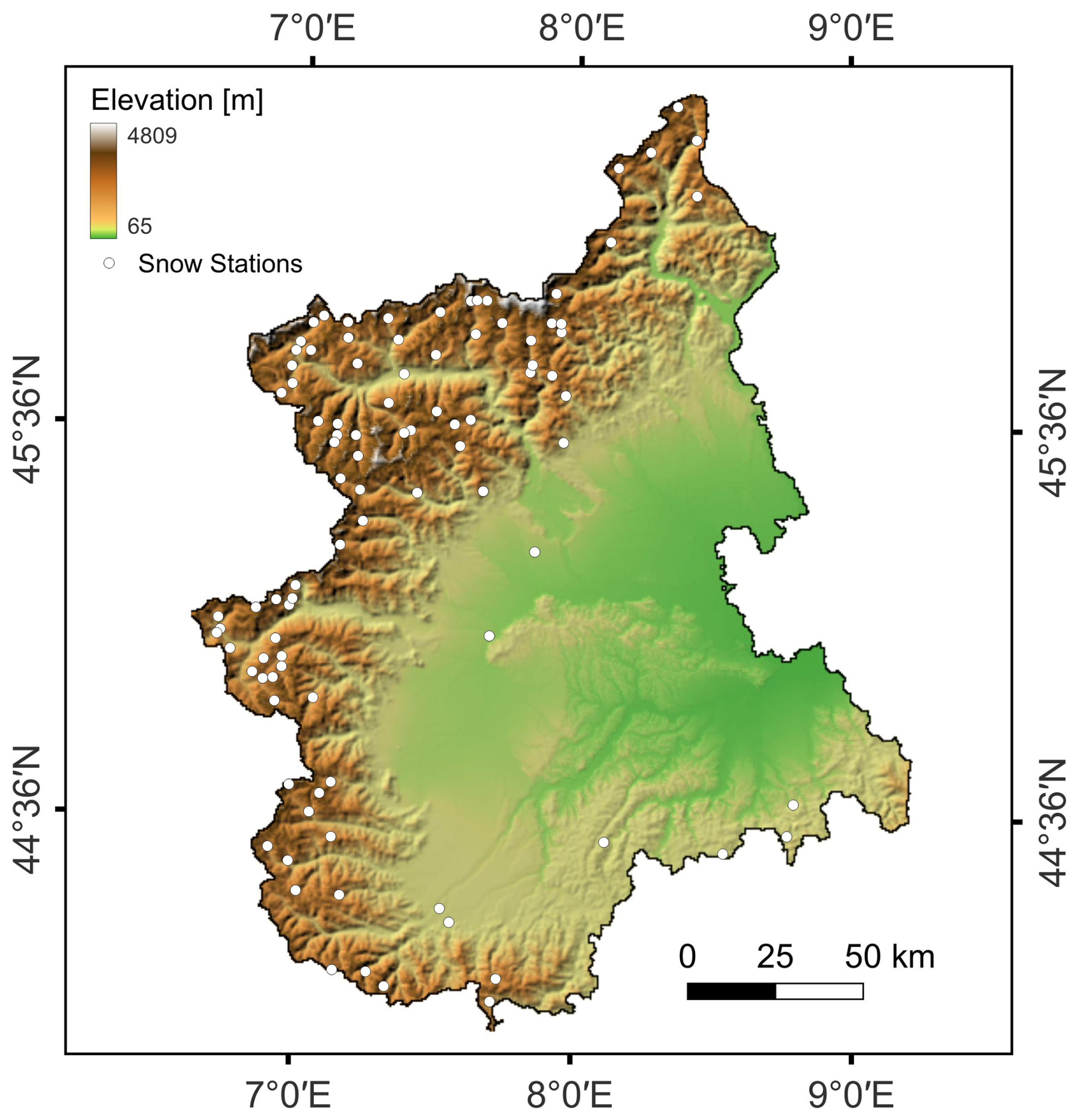
Figure 1 AOI, its morphological complexity and the distribution of the different topographic areas. The white dots represent the snowmeter stations of Arpa Piemonte and Arpa Valle d'Aosta used as ground truth.

Due to the AOI geological/geomorphological asset, the water supply of the lowlands is directly correlated with the water runoff in mountainous areas. In fact, the snow cover offers a natural stock of fresh water during the winter months, and its ecosystem service is necessary to the adequate water recharge of canals and aquifers mainly on the lowlands.

2.2 Data collection

2.2.1 MODIS and Elevation data

MODIS is a satellite mission that provides multispectral imagery with a temporal resolution of 1 d from 2000. In this work, the product MOD10A1.061 Terra was selected and pre-processed in Google Earth Engine (GEE) platform making it possible to monitor the daily evolution of the snow cover at a small scale. In particular, MOD10A1 provides daily snow cover data (in percentage) with a geometric resolution of 500 m (Hall et al., 2002; Liu et al., 2020; Salomonson and Appel, 2004) representing the fraction of the pixel covered by snow. About 8400 images were selected and processed directly in GEE (Gorelick et al., 2017) covering the sensing period between 1 October 2000 and 30 September 2023 over AOI.

This collection product was selected because it was the only long-term MODIS snow dataset (2000–2023) fully available in the GEE catalog. Gap-filled products such as MOD10A1F/MYD10A1F were not accessible in GEE. Moreover, the use of GEE was essential to perform advanced, large-area and dense time-series analyses that would not have been computationally feasible outside the platform.

In order to analyze and correct snow cover data in respect to altitude and terrain slope, the Copernicus DEM GLO-30 (Trevisani et al., 2022) was collected and processed in GEE. Copernicus DEM GLO-30 is a raster layer updated in 2015 that maps altitude data with a geometric resolution of 30 m.

2.2.2 Ground data

The necessity for the ground truth emerged because of the fundamental validation process. The AOI is varied: wide lowlands, hilly areas and mountains of variable elevation, up to an altitude of 4805 m a.s.l. (Mont Blanc). We collected data from snowmeter stations inside the networks of stations of Arpa Piemonte and Arpa Valle d'Aosta (Arpa Piemonte, 2025; Arpa VdA, 2025) covering the entire AOI. The two networks together have more than one hundred stations well distributed throughout the entire territory. To perform this study, it was decided to use 96 stations, all the stations that have dataset for the analyzed period (also partially). The dataset was acquired from the websites of each agency, according to the period of analysis: 1 October 2000 to 30 September 2023. The distribution of the station is visible in Fig. 1.

2.3 Data processing

The workflow adopted in this study is reported in Fig. 2. (1) Data collection step involves collecting and preparing the MOD10A1, terrain data and ground reference samples required for calibrating and testing derived snow products. (2) Data pre-processing step focuses on filtering, masking, and computing snow cover time series and terrain calibration. (3) Processing steps include correcting snow cover area by using DEM data and performing yearly aggregation. (4) Results steps are aimed at statistically quantify snow cover trends and assessing which environmental drivers affect them. Methodological details are described in the next sections.

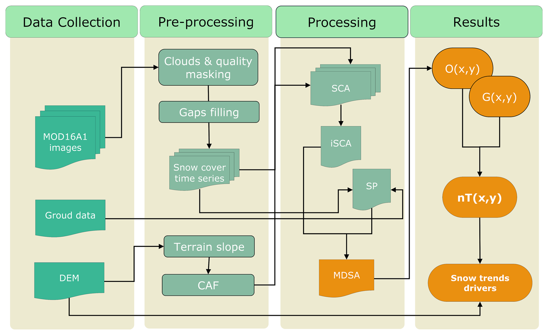
Figure 2 Workflow adopted. Arrows represent the data flow from input data (light green) through methodological steps (in dark green) to the obtained results (in orange).

2.3.1 Mapping Snow Cover Area, Persistence and daily snowed area

Daily snow cover was derived from the MODIS MOD10A1 Collection 6.1 product, which provides fractional snow cover (NDSI Snow Cover, %) at a nominal spatial resolution of 500 m (Hall and Riggs, 2016). The analysis was conducted within Google Earth Engine (GEE). The area of interest (AOI) was defined by merging the administrative boundaries of Valle d'Aosta and Piemonte regions. A digital elevation model (DEM) was obtained from the Copernicus GLO-30 dataset (30 m spatial resolution). The DEM was mosaicked and clipped to the AOI and subsequently reprojected to the native MODIS sinusoidal grid using the projection information extracted from the MOD10A1 NDSI Snow Cover band. The DEM was resampled to 500 m using mean aggregation to ensure spatial consistency with the MODIS data. Terrain slope θ_i was computed from the resampled DEM and used to correct the nominal MODIS pixel area ($A_{\mathrm{p}}=\mathrm{500}\times \mathrm{500}$ m²) for topographic distortion. A correction area factor (CAF) was defined in Eq. (1):

$$\begin{array}{}\text{(1)}& {\text{CAF}}_i={\displaystyle \frac{A_{\mathrm{p}}}{\cos \left({\mathit{\theta }}_i\right)}}\end{array}$$

where θ_i is the local terrain slope at pixel i. The CAF was expressed in hectares, to minimize the unit value of the outcome, aiming to improve computational performance, and applied uniformly to all MODIS observations.

To improve the robustness of the analysis a preventive quality control was done to mask out, date by date, all the critical pixels. The two quality layers provided in the MOD10A1 product were used for this purpose.

The NDSI_Snow_Cover_Basic_QA layer was used to mas out “bad pixels” keeping only Best (code 0) and Good (code 1). Differently, the NDSI_Snow_Cover_Algorithm_Flags_QA layer was used to further mask out those pixels labelled as inland water (bit 0=1), visible screen failure (bit 1=1), NDSI screen failure (bit 2=1), or solar zenith screen failure (bit 7=1).

This masking strategy ensured that only high-quality and physically reliable snow covered pixels entered the analysis, but, in the meantime, generated gaps along the local time series of snow cover. Gap filling was achieved, at pixel level, by linear interpolation operating in the time domain. More complex gap-filling techniques (e.g., splines, LOESS, Savitzky–Golay) were not adopted since are known to oversmooth or generate oscillatory behaviours along the series, especially in heterogeneous mountainous regions (Hird and McDermid, 2009; Jönsson and Eklundh, 2004).

For each pixel and missing observation at time t, snow cover was reconstructed using the closest valid observations before (t₁) and after (t₂) the gap according to Eq. (2).

$$\begin{array}{}\text{(2)}& {\mathrm{\text{NDSI}}}_i\left(t\right)={\text{NDSI}}_i\left(t_{\mathrm{1}}\right)+{\displaystyle \frac{t-t_{\mathrm{1}}}{t_{\mathrm{2}}-t_{\mathrm{1}}}}\left[{\text{NDSI}}_i\left(t_{\mathrm{2}}\right)-{\text{NDSI}}_i\left(t_{\mathrm{1}}\right)\right]\end{array}$$

This approach relies exclusively on observed values and is expected to be conservative, reproducible and limiting the effects of undesired temporal artefacts. Moreover, given the large spatial extent and high temporal density of the dataset, linear interpolation offers the best balance among computational robustness, reproducibility, and physical consistency. This method ensures that derived metrics remain comparable and stable across the study area.

With reference to the gap-filled snow cover time series, the correspondent snow-covered area one (SCA, ha) was computed according to Eq. (3).

$$\begin{array}{}\text{(3)}& {\text{SCA}}_{i,t}={\displaystyle \frac{{\text{NDSI}}_{i,t}}{\mathrm{100}}}\times {\text{CAF}}_i\end{array}$$

Daily SCA maps represent the actual snow-covered surface accounting for slope effects.

Aside this computation, snow persistence was investigated with reference to the hydrological year (1 October–30 September). A binary snow mask, hereinafter called B_i,t, was generated from the NDSI daily maps according to Eq. (4):

$$\begin{array}{}\text{(4)}& B_{i,t}=\left\{\begin{array}{ll}\mathrm{1},& {\text{if NDSI}}_{i,t}>\mathrm{0},\\ \mathrm{0},& \text{otherwise}\end{array}\right.\end{array}$$

The Yearly Snow Persistence (SP, days) was obtained by summing the daily binary masks along the hydrological year, according to Eq. (5):

$$\begin{array}{}\text{(5)}& {\text{SP}}_i^{\left(y\right)}=\sum _{t=\mathrm{1}}^{N_y}(B_i\times \mathrm{\Delta }t{)}_t\end{array}$$

Where N_y is the number of observations in ith hydrological year and Δt_t is the temporal interval in days between consecutive acquisitions. Furthermore, the integrated snow-covered area (iSCA) for each hydrological year was computed as reported in Eq. (6):

$$\begin{array}{}\text{(6)}& {\text{iSCA}}_i^{\left(y\right)}=\sum _{t=\mathrm{1}}^{N_y}({\text{SCA}}_i\times \mathrm{\Delta }t{)}_t\end{array}$$

Finally, the mean daily snow-covered area (MDSA, ha d⁻¹) was defined for each investigated year according to Eq. (7):

$$\begin{array}{}\text{(7)}& {\text{MDSA}}_i^{\left(y\right)}={\displaystyle \frac{{\text{iSCA}}_i^{\left(y\right)}}{{\text{SP}}_i^{\left(y\right)}}}\end{array}$$

This metric represents the average snow-covered area in the yearly period when the snow is present. It is independent from the length of the snow season and allows a robust inter-annual comparison of snow accumulation intensity at the pixel level. Because snow persistence is derived from a binary mask, it is insensitive to sub-pixel reductions in snow-covered areas. Consequently, losses of perennial snow primarily affect iSCA and lead to declining MDSA values even when snow-covered days remain numerous.

2.3.2 Snow Persistence Validation

The environmental preservation service, which in the territories of Piemonte and Valle d'Aosta is carried out by the Arpa agencies, made available, free of charge, the nivometric stations datasets with a time series of nivological metrics, starting from the mid-1900s. These data were used as validation of the working method used for this study. In fact, we compared the single pixel of SP product with the corresponding daily snow presence derived by the snowmeter stations. The process was performed on a yearly basis, in order to obtain a continuous validation dataset for the long-term monitoring period. In this way, it was possible to obtain a curve describing, annually, the amount of days of snow presence on the ground from either station data and data obtained from satellite observation. This process led to a temporal comparison of the amount of days of snow persistence on the ground in order to be able to validate the values obtained from the SP product. We decided to use ground-based meteorological stations as our validation dataset, instead of higher-resolution satellite imagery (such as Landsat or Sentinel products) for several specific reasons. Primarily, the rapid dynamics of snow cover – especially during seasonal transitions – necessitate the daily temporal resolution provided by MODIS, which the revisit times of Landsat and Sentinel cannot currently satisfy. Furthermore, applying higher spatial resolution data to a regional or sub-continental scale introduces significant methodological challenges. Investigating an extensive, predominantly East-West oriented domain like the Alps with Landsat or Sentinel would require mosaicking tiles acquired on different dates. This asynchronicity across the study area would introduce substantial temporal approximations into the analysis that are exceptionally difficult to mitigate.

2.3.3 Snow Cover Trends Quantification

Once MDSA multiannual stack was produced in R vs. 4.1.1 environment, a self-develop routine was implemented in order to analyze at the pixel level the long-term SCC in AOI. In particular, a linear regression was locally fitted involving 23 MDSA values as the dependent variable and the year as the independent one. The slope (Gain) and intercept (Offset) parameters derived by ordinary least squares method (OLS) were mapped into 2 new layers called G(x,y) and O(x,y) having the 500 m of geometric resolution. G(x,y) maps the local increment or decrement of MDSA along the considered period. This value shows the multi-annual trend of a given area to change the daily snow cover. To assess if this trend is significantly different from 0 (i.e., flat trend or not significant changes), a two-tailed t test (Koch, 1999) on slope parameter from OLS was performed involving 22 degree-of freedoms and a significance level of 95 %. All G(x,y) pixels not significant were masked out. Moreover, the determination coefficient of linear regression was also mapped into a new layer called R²(x,y). The latter represents how the linear trend assumption fits the data. Since some areas in AOI may exhibit a quadratic or (high order polynomial) temporal behavior of MDSA, all pixels having $R^{\mathrm{2}}(x,y)<\mathrm{0.5}$ were masked out. This removal allows to guarantee that remaining local trends show linear-like behavior in the considered period making it possible to easily quantify the SCC and future forecasting.

Finally, G(x,y) was divided by O(x,y) in order to create a new layer called normalized trend – nT(x,y). The latter maps the change rate in respect to the year 2000 assumed as reference. This normalization allows to properly compare areas having different environmental starting conditions (e.g., mountain areas vs. lowland ones). In fact, nT(x,y) expresses changes in snow-covered area relative to the local climatological baseline, rather than an individual physical snow event. Using the altitude classification according to Kapos et al. (2000) the nT(x,y) map was divided in 6 groups according to an altitudinal gradient. The Kolmogorov-Smirnov test (KS) (Pratt and Gibbons, 1981) was adopted for assessing the differences among nT values distributions and exploring how altitude can be a driver of SCC in the considered period.

3 Results

3.1 Snow Persistence Validation

The validation process resulted in a good correlation between ground and satellite datasets (Fig. 2).

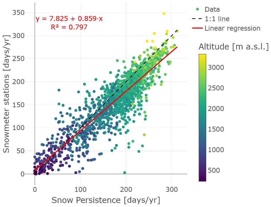
Figure 3 Days of snow persistence calculated by satellite product and ground stations represented in a scatter plot. Dots' colors represent the altitude of the investigated station/pixel. Red line represents the linear regression.

Despite the important geometric difference between the two datasets (500 m vs. single spot), the annual amount of snow persistence was very close. We obtained a R² of 0.8 and a MAE of 20.4. The presence of a minimal offset (Fig. 2) is caused by the geometric difference of the datasets in question: the punctual dataset compared to a 500 m pixel. In fact, in Fig. 4A we can see how the Antrona station, placed at an elevation of 1500 m a.s.l., presents an almost complete overlap of the curves. While in Fig. 4B in the Entracque – Chiotas station, placed at an altitude of 1970 m a.s.l., we can see how the trend of the satellite curve is flat, precisely because of the location of the weather station (above a dam placed on the threshold of a glacial cirque). Furthermore, as is clearly visible in Fig. 3, the clustering of data points around 200 d yr⁻¹ causes the elevation of the offset compared to the points around 50 d yr⁻¹, which closely follow the 1:1 line. This offset is caused by the mean elevation of the stations of around 1783 m a.s.l. and the median of 1905 m a.s.l. This elevation difference increases the impact of the topographic effect in the comparison between point measurement to the 500 m pixel data. This resolution can carry a significant elevation range in mountainous areas. This bias introduces a constant error in the observation and comparison. This error leads to the overestimation of snow presence in mountain areas by the satellite product compared to the ground truth data (Fig. 4B).

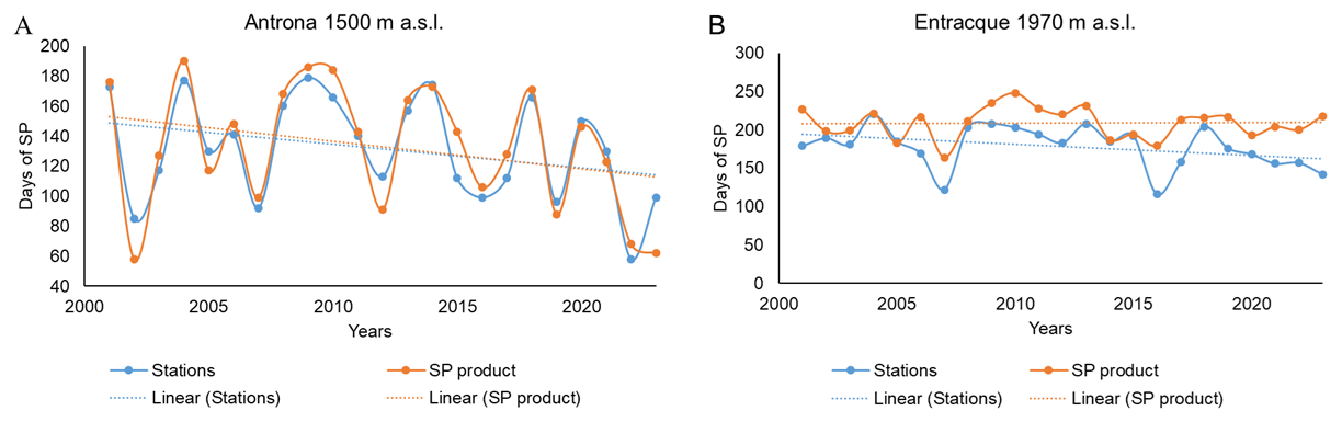
Figure 4 Yearly snow persistence comparing SP measure calculated from MODIS (orange) and ground snowmeter station (blue). (A) Antrona station. (B) Entracque – Chiotas station. In (B) the satellite values (orange) are higher than the station ones (blue) underlighting showing a typical case of overestimation of snow presence.

3.2 Snow Trends Quantification

As introduced in Sect. 2.3.1 and 2.3.3, nT represents a spatial product in which it is possible to assess how snow cover changed from 2000 to 2023 at the Italian Western Alps territory level. The nT product represents the percentage change yearly rate in snow covered area (at pixel level) for a single mean event in respect to t₀ conditions (in the specific case 2000). By normalizing the series with respect to the model intercept we express the gain as a relative change rather than as an absolute value. This operation removes site-specific baseline effects, allowing a consistent and dimensionless comparison of trends across spatially heterogeneous locations. The year 2000 (t₀) is the mathematical origin of the time variable in our model, and serves as a standardized reference point for comparing the relative magnitude of temporal changes across sites.This modeling approach provides a direct and interpretable framework for quantifying and comparing temporal trends across heterogeneous spatial domains. In Fig. 5 it is possible to observe the distribution of the changes in AOI.

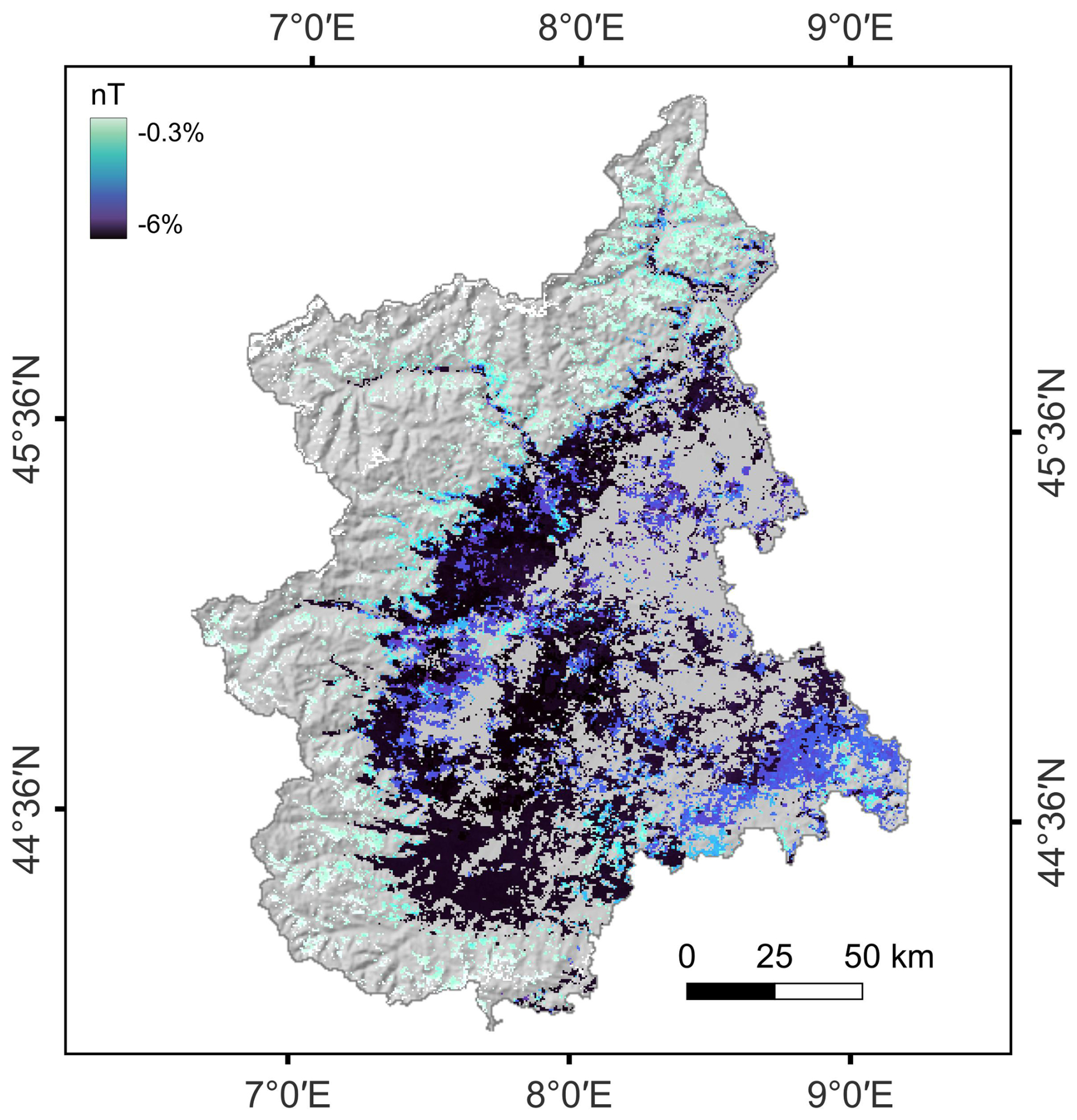
Figure 5 Spatial representation of nT, strongly-negative values are related to low altitude areas, instead of less negative values, related to high altitude areas.

Figure 5 shows nT values in AOI, some areas are not covered because of the masked sectors (as reported in Sect. 2.3.3) that are about 6 % of the total pixel for the not significant gain and 58 % for the low R²(x,y) values. Analyzing Fig. 5, there is a significant trend in the spatial distribution of the obtained values. In fact, the most suffering areas are the ones in the lowlands and main valleys (low altitude sectors in Fig. 1) evidenced by the dark blue colors. This impact seems to reduce moving upward in altitude. The altitudinal trend is well represented in Fig. 6.

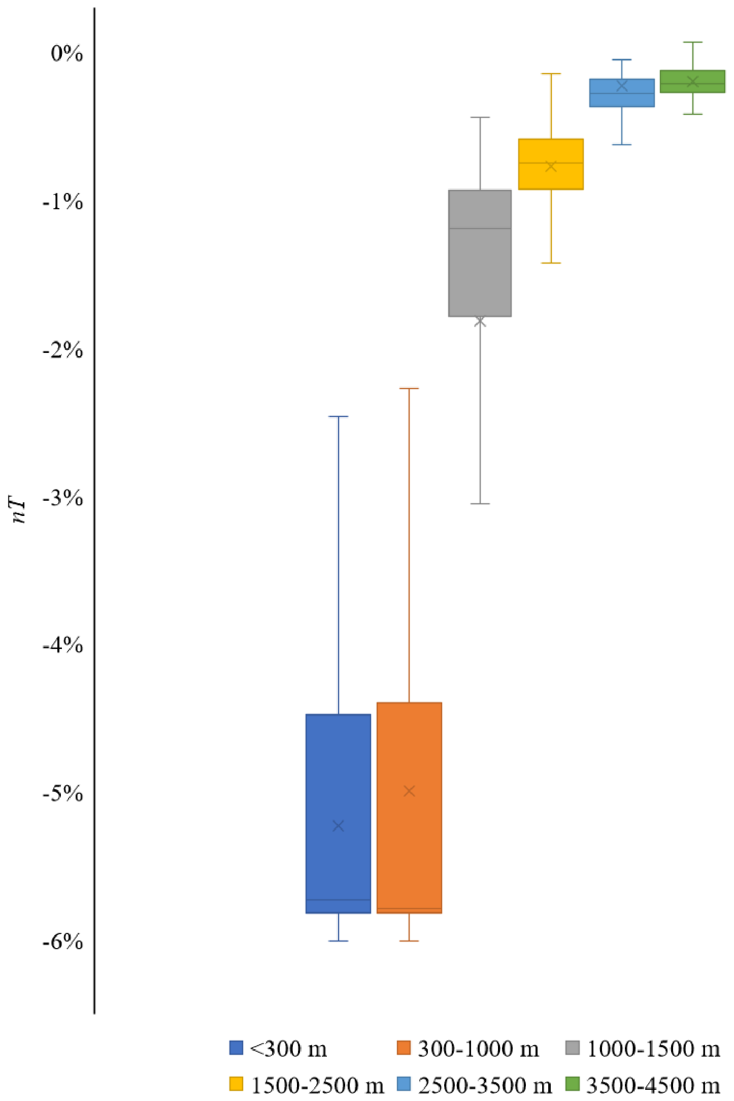
Figure 6 nT in relation to the altitude of the AOI. The values of the altitude reported in meters are in m a.s.l. The altitude classification is taken from Kapos et al. (2000). The boxes are drawn from 25th to 75th percentile with a horizontal line drawn inside it to denote the median and a cross to represent the mean of the data. The whiskers are drawn from the 5th to the 95th percentile.

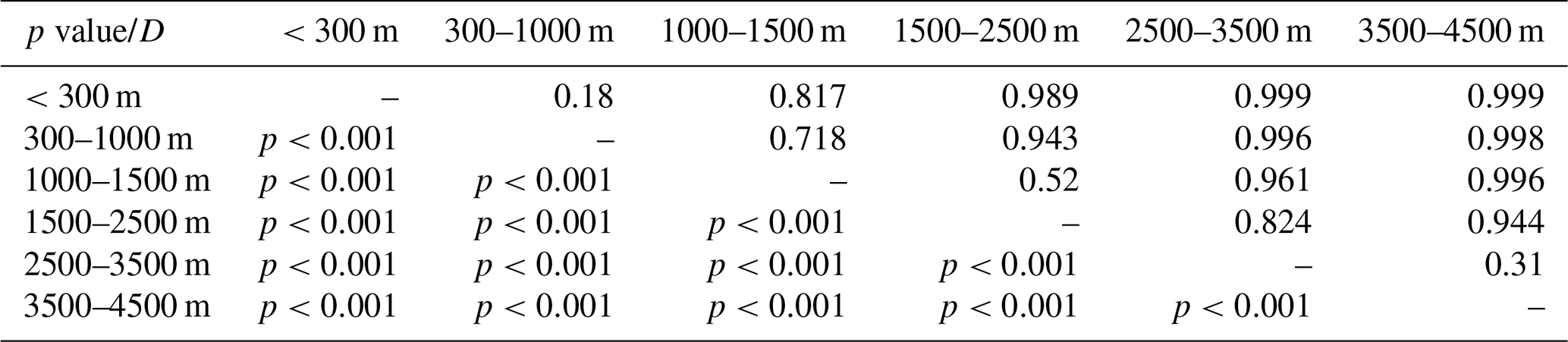
Figure 6 shows the nT values distributions per altitudinal groups. It is worth noting how pixels with high altitude show in general lower nT values. In contrast, pixels on lowland groups show in higher nT supporting the hypothesis of an altitudinal gradient of nT values with the following interpretative key: lowland areas show in general significant negative trends than high mountain ones. The latter have quite flat trends tending to 0. KS test results (Table 1) support this hypothesis denoting significance differences among altitudinal groups.

Table 1 Significance of boxplot in Fig. 6.

4 Discussion

The long-term assessment of snow-cover dynamics in alpine regions requires satellite observations that are both temporally continuous and capable of capturing the full intra-seasonal variability of snow processes. As stated in the introduction, this study aimed to reconstruct the evolution of snow cover (2000–2023) by investigating the potentialities of the MOD10A1 product to assess the intensity of SCC driven by CC. In this context, MODIS stands out as the only Earth observation mission providing a daily and uninterrupted multi-decadal record, which is essential for deriving temporally integrated metrics such as snow persistence, snow-cover duration, and long-term trends. As already reported in Sect. 2.3.2, although higher-resolution missions such as Landsat and Sentinel-2 offer improved spatial detail, their substantially lower revisit frequencies (16 d for Landsat; 2–3 d for Sentinel-2) combined with persistent cloud cover in mountain environments lead to highly discontinuous time series (Gascoin et al., 2015; Parajka and Blöschl, 2008). These limitations introduce major uncertainties when estimating metrics reliant on daily observations, particularly the number of snow-covered days. Furthermore, neither Landsat nor Sentinel currently provides a temporally complete archive comparable to the 23-year MODIS record used in this study. For these reasons, MOD10A1 remains the only dataset capable of supporting long-term, high-frequency analyses of alpine snow climatology, forming a robust foundation for interpreting the time-space patterns.

Results from this study can be used for highlighting the effects of climate warming within the Italian Western Alps due to SCC in the last two decades. In fact, nT synthesizes the percentage variation of snow cover intensity by looking at a single yearly mean snow event. In literature, there are several works that observe phenological changes from satellites: seasonality, persistence, first snowfall (Fugazza et al., 2021; Maskey et al., 2011; Notarnicola, 2020). By introducing the nT concept, we observe the intensity and impact of changes affecting snow cover, on a regional scale, beyond the phenological indexes. nT value makes it possible to summarize the intensity of SCC and enhances the understanding of its evolutionary trends. From the Earth Observation point of view, nT is a good metric to properly compare pixels from different geographic areas. Therefore, it allows to spatialize and describe the effect of the CC in terms of snow cover. nT is independent from the changes of seasonality of the snow (i.e., form the length of snow period). It enhances interpretation of environmental changes through the time, summarizing the changing rate (i.e., G(x,y)) and the starting conditions (i.e., O(x,y)).

Application of nT within the AOI (Fig. 5) highlights clear geo-environmental patterns in the spatial distribution of SCC: the most negative values corresponds to the Cuneo's lowlands, Po Plain and to the main valleys such as Susa Valley, Aosta Valley and Ossola Valley. Moreover, a trend toward more negative values is observed at higher elevations. This altitudinal variation exhibits spatial heterogeneity, as the linear relationship with elevation is likely modulated by latitudinal constraints and geomorphological settings (e.g., topographic aspect, valley proximity, and position within the internal or external zones of the orogen). The most negative values show that the negative trends lead to a complete absence of snow cover. The dark areas in Fig. 5 are showing no more whitening snow events for the last few years. The geo-environmental patterns are well described in Fig. 6. In fact, results of altitudinal classification within the AOI (Fig. 6) shows the extreme impact of nT at low altitudes (below 1000 m a.s.l.) quantified in −5 % per year. In addition, other two areas are strong affected by CC: 1000–1500 m a.s.l. (−1.8 %) and 1500–2500 m a.s.l. (−0.7 %). As mentioned nT shows the changes in snow-whitened areas for a single yearly mean event. This represents that changes are indeed occurring at all elevations, but with greater intensity (in percentage terms, relative to its own mean starting value) at lower elevations. Observing the entire period of nT study, below 1000 m a.s.l. the whitening power of a mean snow event has mostly disappeared and between 1000–1500 m a.s.l. are reduced by more than 40 %.

The observed snow loss at high altitudes, even if it is known that at that elevation the temperature is still below zero degrees, is primarily attributable to two main reasons. Firstly, the increasing air temperatures are frequently driving the zero-degree isotherm to elevations well above the highest peaks in the study area (≈4500 m a.s.l.). This results in non-snow precipitation and extreme melting of the snow during these events. Then, the significant reduction in the extent of perennial snowfields within the study region is also captured by the MODIS snow cover product. Areas that historically maintained permanent snow (e.g., above 3500 m a.s.l.) have experienced substantial ablation and retreat over the 23-year period. This reduction in historically persistent snow contributes to the overall negative nT values, even if the effect is small over a two-decade trend analysis. Therefore, while temperatures remain below zero for much of the year at high altitudes, the increasing frequency of warm-air intrusions and the substantial reduction of permanent snow explain the overall negative, yet often minimal, trends observed in Figs. 5 and 6.

The evolution process, evidenced by nT in Fig. 5, shows that the areas whitened by a single snow event are decreasing. This result offered by the application of our method is a clear representation of the freezing level is moving upward (in elevation) and the decreasing of snow precipitation. The potential snowfall is becoming almost zero at low altitudes (below 1000 m a.s.l.) and very weak in the mid-mountains (1000–1500 m a.s.l.).

Many studies (Avanzi, 2024; Avanzi et al., 2024; Berghald et al., 2025; Bozzoli et al., 2024; Matiu et al., 2021) observed that temperature and precipitation are changing in the AOI. In fact, it is reported that the precipitation are changing in terms intensity (Berghald et al., 2025) and temporal distribution but remaining almost the same for annual value. This effect of the climate emergency, related to the rising temperatures lead to the reduction of the snow season, especially for the areas below 2000 m (Matiu et al., 2021). Recent works (Avanzi, 2024; Avanzi et al., 2024) reported that the drought of the last years affected most, the areas below 1500 m a.s.l. The evidence is underpinned also by nT. As shown in Fig. 6, the more suffering areas were the ones below 1500 m a.s.l., in which the trend is significantly negative. Same negative trend is reported, at a different observation scale, for whole Alpine Region (Bozzoli et al., 2024; Matiu et al., 2021). The spatial distribution of SCC, as highlighted by nT can be of significant value in terms of territorial and water management policies. Many considerations could be derived within the AOI based on our result, from various point of view: land use, tourism, and water resources.

This study presents some limits, the absence of a quantitative volumetric assessment of the observed changes. This limitation represents a significant future research challenge: quantifying snowpack volume necessitates the exploitation of spatiotemporal Snow Water Equivalent (SWE) data. Furthermore, a portion of the study area currently exhibits non-linear or undefined trends in the observed changes. Consequently, repeated temporal observations will be crucial to accurately discern and characterize the evolving dynamics within these specific sectors.

Nevertheless, the findings of this study offer strategic implications for Alpine communities, underscoring the critical importance of effective water resource management across industrial, agricultural, and public consumption sectors. Moreover, in light of the progressive snow cover reduction documented herein, it is imperative to critically evaluate the long-term sustainability of certain winter sports activities at elevations below 1500 m a.s.l.

5 Conclusions

Snow Cover in the Western Alps is undergoing changes that have significant repercussions on the whole sector. Specifically, this study investigated the potentialities of the MOD10A1 product to reconstruct the evolution of snow cover (2000–2023) and assess the intensity of Snow Cover Changes (SCC) driven by Climate Change (CC) in the Italian Western Alps. To achieve this, the herein introduced normalized trend (nT) index quantifies these changes by expressing the annual mean loss of snow cover intensity for an average snow event. Our findings indicate that lowland and main valley areas have undergone the most substantial decrease, with nT values decreasing by up to −5 % below 1000 m a.s.l. and about −1.8 % in areas between 1000–1500 m a.s.l. These findings show the influence of CC on regional snow dynamics, with implications for water resource management. Especially, winter tourism is critically affected by the reduction of snow cover and many winter resorts had to close in the last decades. The long-term sustainability of various economic activities should be re-planned. Also, agriculture should take into consideration the reduction of snow cover as a long-term water supply for the lowlands aquifers to assess future climatic scenarios on water provision.