Sea ice albedo bounded data assimilation and its impact on modeling: a regional approach

We conducted a series of perfect model experiments using Icepack, a one-dimensional single-column sea ice model, to assess the potential of data assimilation (DA) to improve predictions of the mean sea ice state through the incorporation of sea ice albedo (SIAL) observations in addition to sea ice concentration (SIC) and sea ice thickness (SIT) observations. One ensemble member is designated as the TRUTH, and synthetic observations drawn from it are assimilated into the remaining ensemble members. DA is carried out using the Data Assimilation Research Testbed (DART) Quantile Conserving Ensemble Filtering Framework (QCEFF), which accounts for the bounded nature of sea ice variables. Icepack ensembles were spun-up for five Arctic locations based on small perturbations to atmospheric forcing. Results show that assimilating SIAL has the potential to improve reanalysis products when concurrently assimilated with the more commonly assimilated observables SIC and SIT at three of the five discrete points examined in the Arctic Ocean, when observational uncertainty in SIAL is reduced below current literature estimates. These findings underscore the value of leveraging existing SIAL observations and expanding their temporal and spatial coverage in the Arctic. Furthermore, the study highlights the critical need to better constrain the observational uncertainty of SIAL. Enhanced observational networks would provide the necessary validation data, enabling more accurate uncertainty characterization and improving sea ice forecasts in a rapidly evolving polar climate.

1 Introduction

Arctic amplification refers to the phenomenon in which the Arctic experiences accelerated warming compared to the global average. This enhanced warming has been consistently observed over recent decades (Rantanen et al., 2022). The accelerated warming is partially attributed to the ice-albedo feedback mechanism, in which the melting of snow and sea ice exposes darker underlying surfaces, enhancing the absorption of short-wave radiation and further amplifying ice loss (Perovich and Polashenski, 2012; Serreze and Barry, 2011). Despite the critical role of this feedback in the dynamics of Arctic climate, global climate models (GCMs) exhibit persistent limitations in accurately simulating Arctic sea ice. These deficiencies contribute to significant uncertainties in the projection of key sea ice variables, including sea ice concentration (SIC), sea ice thickness (SIT), and surface albedo (Donohoe et al., 2020; Pithan and Mauritsen, 2014).

Sea ice albedo (SIAL) is defined as the fraction of incoming solar radiation reflected back into the atmosphere in ice-covered regions of the polar oceans. In practice, SIAL and SIC frequently co-vary in response to sea ice retreat (Agarwal et al., 2011), yet SIAL also carries independent information about surface properties that SIC alone cannot capture such as melt ponding and snow loss. Bare sea ice exhibits a relatively high albedo, typically reflecting 50 %–70 % of incident short-wave radiation (Grenfell and Perovich, 2004), in stark contrast to the open ocean, which only reflects about 10 %, absorbing most of the incoming short-wave radiation due to its much lower albedo (Becker et al., 2023). Snow-covered sea ice can reflect 90 % of incoming short-wave radiation, whereas melt ponds, which form on the ice surface during the melt season, exhibit highly variable albedo values. These values depend on factors such as pond depth and water clarity, often resulting in significantly lower albedo relative to bare ice (Grenfell and Perovich, 2004; Perovich, 1996). The spatial and temporal variability of SIAL – driven by changes in surface conditions on the sea ice, such as snow cover, bare ice, and melt ponding – modulates the amount of solar radiation reflected within ice-covered regions. SIAL is typically derived from satellite top of atmosphere (TOA) remote sensing, which enables spatially extensive, long-term observations, but it is also measured directly via in-situ instruments deployed on the ice, offering higher-resolution insights into local surface conditions (Karlsson et al., 2023; Calmer et al., 2023). While the primary ice–albedo feedback arises from the strong contrast between sea ice and open ocean albedos, variability in SIAL governs the intensity and spatial distribution of this feedback over ice-covered areas such as the Central Arctic. Accordingly, SIAL serves as an important regulator of the Arctic shortwave radiative balance, particularly during the summer melt season (Seong et al., 2022; Arndt and Nicolaus, 2014).

The primary aim of this study is to improve the accuracy of sea ice reanalysis simulations by integrating idealized albedo observations within an ensemble data assimilation (DA) framework using synthetic (perfect model) experiments. Assimilating SIAL observations offers a potential pathway to refine the representation of modeled energy exchange processes, reducing uncertainties in simulations of Arctic sea ice. While this study serves as a proof-of-concept demonstration under idealized conditions, such an approach has the potential to inform future improvements in model parameterizations related to ice surface properties, ice thermodynamics, and ice thickness distributions (Hunke et al., 2010; Lindsay, 2001; Barry, 1996).

The inclusion of SIAL in the DA framework is expected to improve the ability of the model to capture interannual variability and very rapid sea ice loss events (VRILEs) within the marginal ice zone (MIZ), which are essential to understand the rapid sea ice transformations that occur in the Arctic (Cavallo et al., 2025; Pistone et al., 2014; Schröder et al., 2014; Perovich et al., 2008). By addressing deficiencies in SIAL representation through idealized DA experiments, this study aims to lay the groundwork for future improvements in subseasonal-to-decadal sea ice forecasting skill and projections of Arctic sea ice trends.

2 Methods

To quantify the impact of SIAL DA, we conducted a series of perfect-model experiments using the Icepack sea ice model (v1.4.0; Hunke et al., 2023), the thermodynamic module of the widely used Community Ice CodE (CICE). Icepack is a one-dimensional, column-based model that simulates vertical thermodynamic processes in sea ice but does not include horizontal ice dynamics such as advection. For this study, Icepack was spun up from 2000 to 2010 to establish realistic local ice conditions in five key Arctic regions: the Barents Sea (75° N, 40° E), the Beaufort Sea (70° N, 140° W), the Central Arctic (88° N, 0° E), Coastal Canada (81° N, 2° W), and the Siberian–Chukchi Sea (76° N, 174° E). This 11-year spin-up period allows the model to equilibrate to prescribed atmospheric and oceanic forcing, eliminating artifacts from idealized initial conditions and ensuring that all subsequent simulations begin from physically consistent and realistic ice states. The early 2000s were selected as a critical transition period in Arctic sea ice history, during which the region began shifting from a predominantly multi-year ice cover to one dominated by first-year ice (Sumata et al., 2023). Each Icepack simulation was forced with prescribed atmospheric conditions from the Japanese 55-year Reanalysis for driving ocean–sea-ice models (JRA-55-do, see below) and coupled to a slab ocean, following Tsujino et al. (2018). Initial conditions for the slab ocean were derived from the ocean component output of a fully coupled historical simulation using the Community Earth System Model (CESM2). For each region, we generated an ensemble of 30 Icepack simulations to capture internal variability and provide a basis for subsequent ensemble-based DA experiments.

Our ensemble was generated solely by perturbing external atmospheric forcing fields, following Appendix A of Wieringa and Bitz (2025), which ensures that perturbations retain realistic spatiotemporal coherence between atmospheric variables. In practice, this is achieved by perturbing the left singular vectors of the covariance matrix of the atmospheric state, such that the resulting ensemble members remain statistically consistent with the reference forcing fields. For every member, a unique namelist file was created by perturbing selected atmospheric forcing fields (temperature, specific humidity, zonal and meridional wind, short- and longwave fluxes, and precipitation) using the JRA-55-do reanalysis data. The ocean forcing remained identical across the ensemble. All ensemble members shared a common ocean forcing to ensure that ensemble spread arose primarily from atmospheric forcing perturbations. Icepack parameters were also held constant across experiments, and are included in the Supplement (Table S3).

All members were integrated forward for the spin-up period using consistent external boundary conditions, after which restart files were generated at the end of 2010. These restart states served as the initial conditions for the assimilation experiments. Model output was collated across ensemble members, resampled to daily means, and combined into a single dataset with ensemble dimension. Ensemble mean and spread were calculated and stored in separate NetCDF files for subsequent analysis.

Icepack parameterizes the ice thickness distribution (ITD) by discretizing the continuous range of sea ice thicknesses into n distinct thickness categories (with n=5 in our integrations). The model state variables – aice_n (ice area), vice_n (ice volume), and vsno_n (snow volume) – are defined for each thickness category and are normalized by the grid-cell area. This categorization allows the model to capture the heterogeneous and nonlinear behavior of sea ice processes across the thickness spectrum, enabling physically consistent thermodynamics and parameterized mechanical interactions (e.g., ridging and rafting) for thin versus thick ice.

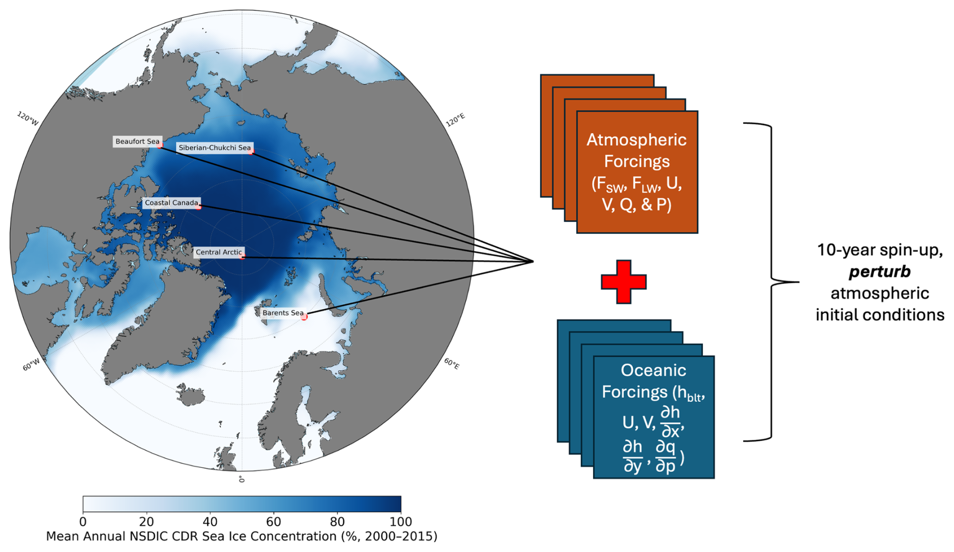
Figure 1 Geographic locations of the atmospheric and oceanic forcing selected for analysis. Atmospheric forcings used to spin up the sea ice ensemble include downwelling shortwave (F_SW) and longwave (F_LW) radiation (W m⁻²), 10 m zonal (U) and meridional (V) wind speeds (m s⁻¹), specific humidity (Q, kg kg⁻¹), and precipitation (P, kg m⁻² s⁻¹). Oceanic (slab) forcings include temperature (T, K), salinity (S, PSU), mixed layer depth (h_blt, m), surface zonal and meridional currents (U, V, m s⁻¹), ocean surface tilt ($\partial h/\partial x$, $\partial h/\partial y$; unitless), and vertical convergence of heat transport ($\partial q/\partial p$, W m⁻³).

We selected geographic locations (Fig. 1) to assess how SIAL assimilation influences the modeled sea ice behavior in different Arctic regions, with a particular focus on how local atmospheric forcings shape ice evolution in areas with varying sea ice regime climatologies (e.g., thick, perrenial ice, seasonal first-year ice, landfast ice) (Tschudi et al., 2020; Serreze and Barry, 2011). We overlay mean annual SIC (2000–2015) from the National Snow and Ice Data Center (NSIDC) Climate Data Record (CDR) for a greater understanding of typical ice conditions at these five locations (Meier et al., 2024).

The spun-up ensembles were then integrated forward for a 5-year period (2011–2015) without any DA. The 5-year period following spin-up was selected to balance two goals: ensuring a long enough time window to evaluate the cumulative impact of DA on sea ice state evolution, while remaining short enough to minimize the influence of structural model drift and changes in climate forcing not represented by the perfect-model framework. This period also aligns with the availability of well-characterized reanalysis inputs and avoids strong interannual anomalies that could dominate the signal. Additionally, using a relatively short post-spin-up period helps isolate the effects of initial condition uncertainty and DA rather than external forcing trends. This free run serves as a control case against which assimilation experiments can be evaluated. For each assimilation experiment – defined as the set of simulations conducted for one of the five Arctic locations – a randomly selected ensemble member was designated as the reference TRUTH state, from which synthetic observations were derived for assimilation. To account for sensitivity to the choice of TRUTH, we repeated the assimilation experiments using eleven different ensemble members as TRUTH states (ensemble members 3, 5, 8, 10, 12, 14, 16, 19, 21, 25, and 28). Synthetic observations of SIAL, SIC, and SIT were generated from each of these TRUTH realizations for assimilation into the remaining ensemble members. Using synthetic observations is advantageous as they share the same spatial and temporal scales as the model. Moreover, in a one-dimensional framework, these observations can be assimilated and tested for significance with substantially lower computational cost compared to assimilating real observations that are not co-located with the model column.

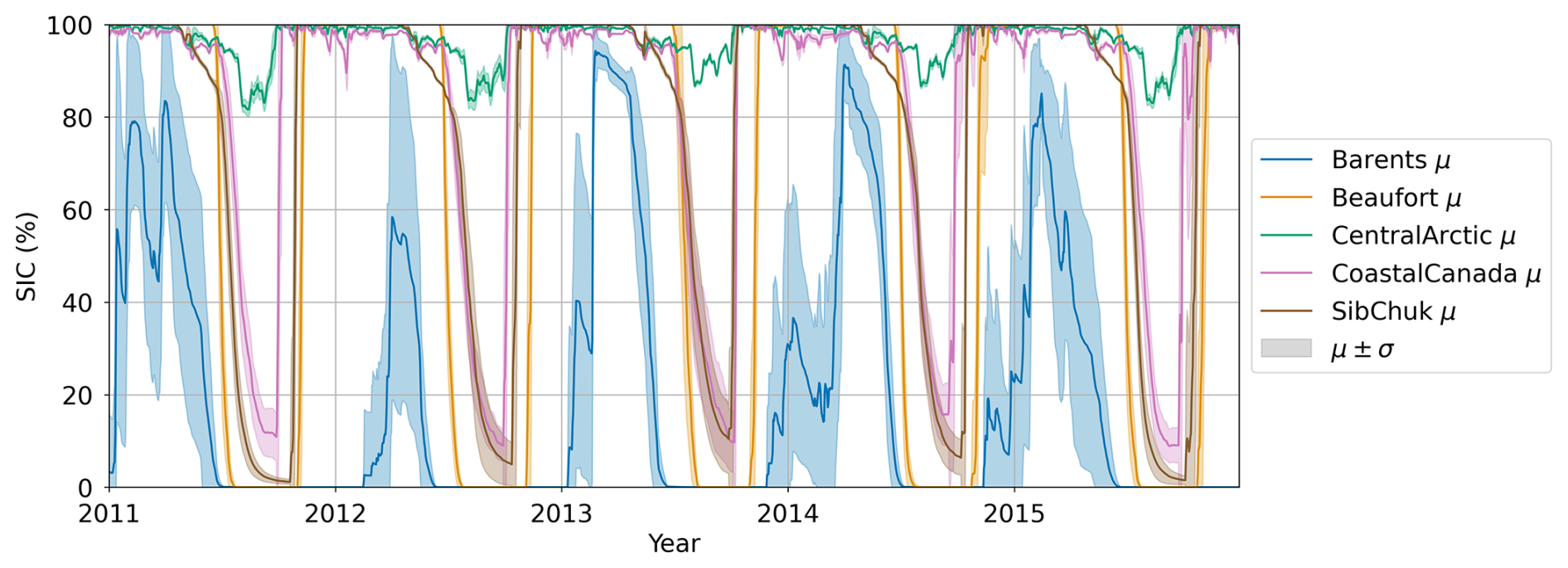
Figure 2 Mean (μ) and standard deviation (±σ) of SIC across ensemble members and region of the Icepack free-run for 2011–2015.

Figure 2 presents the ensemble mean (μ) SIC in the free run at each selected location for 2011–2015, along with the ensemble spread indicated by ensemble standard deviation (±σ). The Barents Sea location exhibits the highest variability in SIC across the study period and does not reach full ice coverage in the ensemble mean. The Siberian–Chukchi Sea also displays a highly seasonal SIC cycle, achieving near-complete coverage during winter but retreating substantially in summer. Both regions lie within the marginal ice zone (MIZ), where sea ice frequently transitions between open water and partial coverage. To represent these dynamic conditions, we configure these sites in Icepack using the fluxing open water boundary condition. In standalone Icepack simulations, this functionality is required to approximate the exchange of energy and mass between sea ice and the surrounding ocean, particularly in regions with seasonally variable ice cover. Without a dynamic coupling to an ocean model, Icepack must either assume uniformly ice-covered conditions (fluxing uniform ice) or allow for partially open water that can receive and exchange fluxes at the ice edge. The fluxing open water option provides a more realistic treatment of MIZ dynamics in these seasonally ice-covered regions.

The Coastal Canada region exhibits a pronounced seasonal signal but remains partially ice-covered even during the summer minimum. Because Icepack does not include coastlines or ice advection, it cannot represent the coastal ice buildup that is well captured in observations and full three-dimensional sea ice models. As a result, SIC values in this region are likely underestimated. In contrast, the Central Arctic is dominated by perennial, multi-year ice and exhibits minimal seasonal variability in SIC, making it a stable reference point for comparison. Together, these two sites span distinct environmental regimes yet are each configured to represent fluxing uniform ice – locations where sea ice dynamics are governed primarily by internal redistribution and deformation within a contiguous ice pack rather than by interactions with open water or ice-edge processes.

The Beaufort Sea site was selected to represent landfast ice, where local geometry and coastal boundaries suppress drift and promote seasonally persistent ice. These conditions are predominantly thermodynamic in nature and therefore more compatible with standalone Icepack simulations (Plante et al., 2024). To reflect the low mobility of landfast ice, the deformation rates at this location were set to zero. As a result, no sea ice or open water fluxes into this site, which is thus treated as a strictly thermodynamic column.

At all other cites, deformation rates in Icepack are prescribed based on estimates by Lindsay (2002) made for perennial sea ice during the Surface Heat Budget of the Arctic Ocean (SHEBA) field campaign as previously used in Wieringa and Bitz (2025). When imposed in regions with seasonal sea ice, these deformation rates produce too little deformed ice and therefore cause excessive level ice cover.

To reduce the impact of errors in the level ice fraction, we applied different melt pond parameterizations depending on region. The level melt pond scheme was used in the Barents Sea, Beaufort Sea, and Central Arctic, where it is assumed to improve albedo representation and produced realistic seasonal melt evolution in our simulations based on past literature (Hunke et al., 2013). However, in the Coastal Canada and Siberian–Chukchi Seas, the level scheme led to albedo evolution that significantly diverged from observational constraints. In these two regions, we therefore applied the empirical topographic melt pond scheme, which has been used in several Coupled Model Intercomparison Project Phase 6 (CMIP6) models (Keen et al., 2021) and yielded better agreement with observed albedo variability.

A full physical explanation for the differing regional behavior is provided in the Supplement (see Sect. S6 and associated Fig. S3), but we note here explicitly that the melt pond scheme configuration differs by region as described above.

2.1 Data Assimilation Setup

One of the most challenging aspects of sea ice DA is the inherent boundedness of the modeled variables. Quantities such as SIAL (bounded between 0 and 1), SIC (modeled as a fraction from 0 to 1, reported here as 0 %–100 %), and SIT (≥ 0 m) pose limitations on the potential ensemble spread, especially during periods when these variables approach their physical bounds – typically in winter (near-maximum values for SIC) and summer (near-minimum values for SIC and SIT). During transition seasons, SIAL and SIC can also exhibit rapid nonlinear changes due to melt pond formation, refreezing, snowfall, and other surface processes. In such cases, the model ensemble may lack sufficient variability to adequately represent fast seasonal transitions, making it difficult for traditional DA methods, many of which rely on unbounded Gaussian assumptions, to optimally update the model state. These limitations necessitate alternative assimilation frameworks that explicitly account for physical bounds and distribution asymmetries.

To address these challenges, we employed the Quantile Conserving Ensemble Filtering Framework (QCEFF; Anderson et al., 2024; Anderson, 2022), implemented within the Data Assimilation Research Testbed (DART; Anderson et al., 2009). DART is a community DA system developed by the Data Assimilation Research Section (DAReS) of the National Center for Atmospheric Research (NCAR) with the support of the National Science Foundation (NSF). Specifically, we used the bounded normal variant of the Rank Histogram Filter (BNRH; PQBNRH in Anderson et al., 2024), which combines the statistical rigor of Gaussian-based assimilation with the physical realism of bounded state variables. The filter works by fitting a rank histogram distribution with truncated normal tails to the ensemble, conserving rank-based quantiles during the update step while ensuring that the resulting values remain within physically plausible limits. This approach has been shown to improve the performance of DA systems when dealing with constrained geophysical variables, as it prevents nonphysical ensemble updates (e.g., SIAL > 1 or negative SIT; Riedel et al., 2025; Anderson et al., 2024; Wieringa et al., 2024).

SIAL assimilation, in particular, benefits substantially from this bounded framework. Unlike SIC and SIT, which frequently approach their lower or upper physical limits, SIAL values typically remain within a central range – rarely falling below 0.1 or exceeding 0.9 – even during extreme seasonal transitions. This characteristic makes SIAL an ideal candidate for assimilation within a truncated Gaussian filter, as the ensemble spread is more likely to encompass the true state without frequently encountering hard boundaries. As a result, the BNRH can fully leverage its quantile-conserving properties without being regularly constrained by the extremes of the distribution. Unfortunately, within Icepack, SIAL is set to “0” when SIC is 0 % and to “1” during winter when solar radiation is absent, so these potentially advantageous features of SIAL are only partially applicable in this perfect model framework.

While this bounded formulation has recently been applied to SIC and SIT (e.g., Riedel et al., 2025; Wieringa et al., 2024), its implementation for SIAL assimilation is novel. Assimilating in Icepack with the QCEFF method allows for a more consistent and physically grounded incorporation of SIAL and other bounded observations, underscoring the potential of bounded DA algorithms to advance the prediction capabilities of sea ice systems.

2.2 Observations

Synthetic observations assimilated by DART are generated by adding random noise drawn from a truncated normal distribution with a standard deviation of σ, centered on the TRUTH value. The resulting values are then clipped to ensure they remain within physical bounds (e.g., SIAL between 0 and 1). A sensitivity test examining the influence of random observational noise realizations on assimilation performance is included in the Supplement (Fig. S1). This process accounts for uncertainties that would affect real-world observations of the selected variables (Anderson et al., 2024). The synthetic observations are calculated as aggregates of modeled quantities from Icepack that are binned by ice-thickness category (e.g., aice_n, vice_n). Most in-situ observations, by contrast, are point measurements of single variables such as SIT or SIC, which are typically treated as diagnostic quantities in sea ice models. In one experiment, we depart from this aggregate framework and instead assimilate synthetic SIAL observations separately within each thickness category – that is, we provide the DA system with SIAL values corresponding to each modeled category, SIAL_n. This allows us to investigate the role of modeled SIAL across the thickness categories in assimilation performance, particularly in the Siberian–Chukchi Sea region, where the standard approach underperforms (see Sect. 2.5 for more details).

The synthetic observation types used in our DA experiments include SIC, SIT, and four SIAL components derived from Icepack's narrow-band albedo scheme: direct visible (α_DirVis), direct infrared (α_DirIR), indirect visible (α_IndVis), and indirect infrared (α_IndIR). These observations are calculated as aggregates over the model's thickness categories based on quantities such as aice_n and vice_n. In our configuration, which uses Icepack's 3-band Delta-Eddington radiative transfer scheme (shortwave = ‘dEdd’), the model sets direct and diffuse shortwave fluxes equal, eliminating the need to treat them separately. However, the scheme retains separate visible and infrared spectral bands because albedo and absorption differ strongly between these wavelength ranges. Consequently, albedo observations are grouped into two spectral bands – visible (α_Vis) and infrared (α_IR) – for analysis. While Icepack supports a more spectrally resolved 5-band scheme, it was not used in this study. The simplification is consistent with both the 3-band scheme's structure and the high correlation observed between direct and indirect albedos in version 1.4.0 (CICE Consortium, 2025).

Table 1 Observation types, forward operators, and prescribed observational uncertainty assumptions are defined to ensure consistency with current satellite sea ice products. The SIAL aggregates are weighted by sea ice area.

The prescribed observational uncertainty distributions for each synthetic observation are summarized in Table 1 and visualized in Appendix Fig. A1. The synthetic observational uncertainties listed in Table 1 were specified based on values reported in previous literature. For the narrow-band aggregate SIAL observations (α_DirVis, α_DirIR, α_IndVis, and α_IndIR), three levels of observational uncertainty were adopted, informed by estimates from Riihelä et al. (2024) and Xiong et al. (2002). These three uncertainty levels – ±5 %, ±14 %, and ±25 % – reflect the limited validation data available for satellite-derived SIAL observations and are intended to represent low, medium, and high uncertainty scenarios, respectively. The few existing in-situ validation studies suggest that actual satellite observational retrieval uncertainties are likely closer to the low-to-medium uncertainty range (Riihelä et al., 2010; Xiong et al., 2002).

The observational uncertainty for aggregate SIC is modeled as a negative parabola (Table 1), with the greatest uncertainty occurring within the MIZ, where SIC ranges between 15 % and 85 %. This formulation reflects current understanding that satellite retrievals of very low or very high SIC are generally more accurate than those within the MIZ, where spatial heterogeneity and measurement limitations introduce greater uncertainty (Wernecke et al., 2024; Han et al., 2021; Brucker et al., 2014). It is important to note that this uncertainty parameterization can also depend on surface conditions such as snow cover and the presence of melt ponds, which are not explicitly included in our uncertainty calculations, but are instead solely dependent on SIC.

Similarly, the observational retrieval uncertainty for aggregate SIT is informed by satellite observation campaigns such as the Ice, Cloud, and land Elevation Satellite-2 (ICESat-2) and CryoSat-2. For simplicity, the SIT uncertainty is approximated as 10 % of the observed value (Table 1), which likely underestimates the true observational uncertainty and should be interpreted as a lower bound, consistent with prior estimates (Zhang et al., 2023; Stonebridge et al., 2018). It should be noted that this relationship may not hold at very low SIT values, where sea ice freeboard becomes small or even negative, introducing greater observational challenges (Rösel et al., 2018). Additionally, this somewhat arbitrary choice of uncertainty is likely optimistic – uncertainties from older SIT observational datasets are considerably larger (e.g., Schweiger et al., 2011).

2.3 Assimilation Temporal Selection

The DA methodology involved assimilating daily synthetic observations from 1 April to 15 October 2011. The temporal range – from spring through early autumn – was selected to align with the period during which satellite-derived SIAL observations are available and solar radiation effectively reaches the high Arctic, enabling reliable SIAL retrievals. This also coincides with the season when SIAL plays a key radiative role; during winter, limited solar insolation renders SIAL variations largely inconsequential to the surface energy budget. DA was similarly conducted for 2012–2015 melt seasons and produced qualitatively similar results (not shown).

Daily observational SIAL products are available from the Polar Pathfinder (APP-x) dataset, which uses data from the Advanced Very High Resolution Radiometer (AVHRR) sensor (Tschudi et al., 2019). Consequently, the temporal sampling frequency for synthetic observations in the assimilation was matched to this daily resolution to enable future comparisons with APP-x. However, it should be noted that other operational products, such as the CLARA-A3 dataset from the EUMETSAT CM SAF, provide SIAL estimates at a pentad (5 d) resolution. This coarser temporal frequency reflects the need to combine observations in order to mitigate the effects of low solar elevation and oblique satellite viewing angles, which amplify bidirectional reflectance distribution function (BRDF) related uncertainties and complicate the feasibility of truly daily SIAL retrievals, particularly in polar regions (Riihelä et al., 2024).

While daily assimilation of variables like SIAL and SIT is useful for idealized benchmarking, assuming the availability of fully gridded daily observations may not align with current satellite capabilities. SIAL retrievals depend on favorable surface illumination and low cloud cover, while SIT estimates – though available along satellite tracks at daily resolution – require radar or lidar altimetry, which have limited spatial coverage and higher uncertainty during melt conditions or over thin ice (Karlsson et al., 2023; Petty et al., 2023). Future work should explore the impacts of more realistic observational sampling frequencies to better reflect operational constraints.

2.4 Error Metrics

The primary metric used to evaluate assimilation performance is the Root Mean Square Error (RMSE), chosen for its robustness and interpretability. RMSE is particularly effective because it is sensitive to large errors, thereby highlighting substantial discrepancies between μ and the designated TRUTH member. It has also been widely adopted in previous sea ice DA studies (Williams et al., 2023; Zhang et al., 2021). Additionally, RMSE yields a single scalar value that captures the overall magnitude of error, facilitating direct comparisons across different assimilation configurations.

For completeness, the mean absolute error (MAE) was also calculated, which yielded results that were qualitatively similar to those from RMSE (not shown). However, RMSE is prioritized here because large deviations, specifically, cases where μ strays ≥2σ from the synthetic observational TRUTH, can indicate observation rejection. This effectively results in a secondary ensemble free-run, which may diverge even further from the TRUTH than the control simulation.

Importantly, RMSE accounts for both systematic errors (bias) and random errors (variance), offering a comprehensive measure of model performance. This holistic evaluation ensures that consistent and unpredictable errors are reflected in the metric. The RMSE is computed as follows:

$$\begin{array}{}\text{(1)}& \mathrm{RMSE}=\sqrt{{\displaystyle \frac{\mathrm{1}}{N}}\sum _{i=\mathrm{1}}^N{\left(y_i-{\widehat{y}}_i\right)}^{\mathrm{2}}},\end{array}$$

where N is the total number of data points, y_i is the observed value at time i, and ${\widehat{y}}_i$ is the corresponding predicted or modeled value. The summation is taken over the daily data points spanning the full assimilation period from 1 April to 15 October, which corresponds to N=198 time instances.

To assess the robustness of assimilation performance, RMSE was computed separately for eleven distinct ensemble members, each randomly selected to serve as a synthetic TRUTH in separate experiments. These eleven TRUTH realizations were drawn from the same prior ensemble used in the assimilation cycles, ensuring internal consistency. By evaluating RMSE across multiple TRUTHs, we account for natural variability in the system and avoid overfitting our results to a single realization. The reported RMSE values therefore reflect the mean performance across these eleven cases, with 95 % confidence intervals derived via bootstrap resampling. This multi-TRUTH framework supports a more generalized evaluation of each assimilation configuration.

To quantify the relative advantage of incorporating SIAL observations with SIC and/or SIT, we compare assimilation configurations using SIC-only, SIT-only, and combined SIC-and-SIT setups by calculating the percent RMSE difference. This metric measures how much more (or less) effective adding SIAL is at reducing RMSE compared to the other configurations, with all differences referenced to a free-running control simulation (Fig. 2). The metric is defined as:

$$\begin{array}{}\text{(2)}& \begin{array}{rl}\mathrm{\Delta }\mathit{\%}{\mathrm{Diff}}_{\mathrm{SIC}/\mathrm{SIT}}& =\left({\displaystyle \frac{{\mathrm{RMSE}}_{\mathrm{SIAL}+}-{\mathrm{RMSE}}_{\mathrm{ctrl}}}{\left|{\mathrm{RMSE}}_{\mathrm{ctrl}}\right|}}\right)\times \mathrm{100}\\ & -\left({\displaystyle \frac{{\mathrm{RMSE}}_{\mathrm{SIC}/\mathrm{SIT}}-{\mathrm{RMSE}}_{\mathrm{ctrl}}}{\left|{\mathrm{RMSE}}_{\mathrm{ctrl}}\right|}}\right)\times \mathrm{100}.\end{array}\end{array}$$

A negative value of this metric indicates that adding SIAL to the DA update variables resulted in greater RMSE reductions than SIC and/or SIT assimilation, whereas a positive value indicates poorer performance. This approach allows a direct comparison of the added value of SIAL assimilation across experiments, observational uncertainty levels, and regions.

2.5 Category-Wise Data Assimilation

Category-wise DA refers to the assimilation of a variable independently within each category of the ice thickness distribution represented in Icepack. Although this approach is not applicable in real-world settings – since current observational systems cannot resolve sub-grid-scale ITDs – it is particularly valuable in perfect model experiments. Such an approach helps identify underlying causes for unexpected assimilation outcomes, such as cases where assimilation leads to an increase in ensemble mean RMSE relative to the free run in our model configuration.

3 Icepack Variable Relationships

We begin by examining the relationships among all Icepack aggregate variables of interest across all regions to assess their uniqueness and find where there is overlap over the melt season that we defined as 1 April–15 October (Fig. 3). We find that many variables are strongly correlated with each other. In particular, SIAL is well correlated with SIC but less so with SIT.

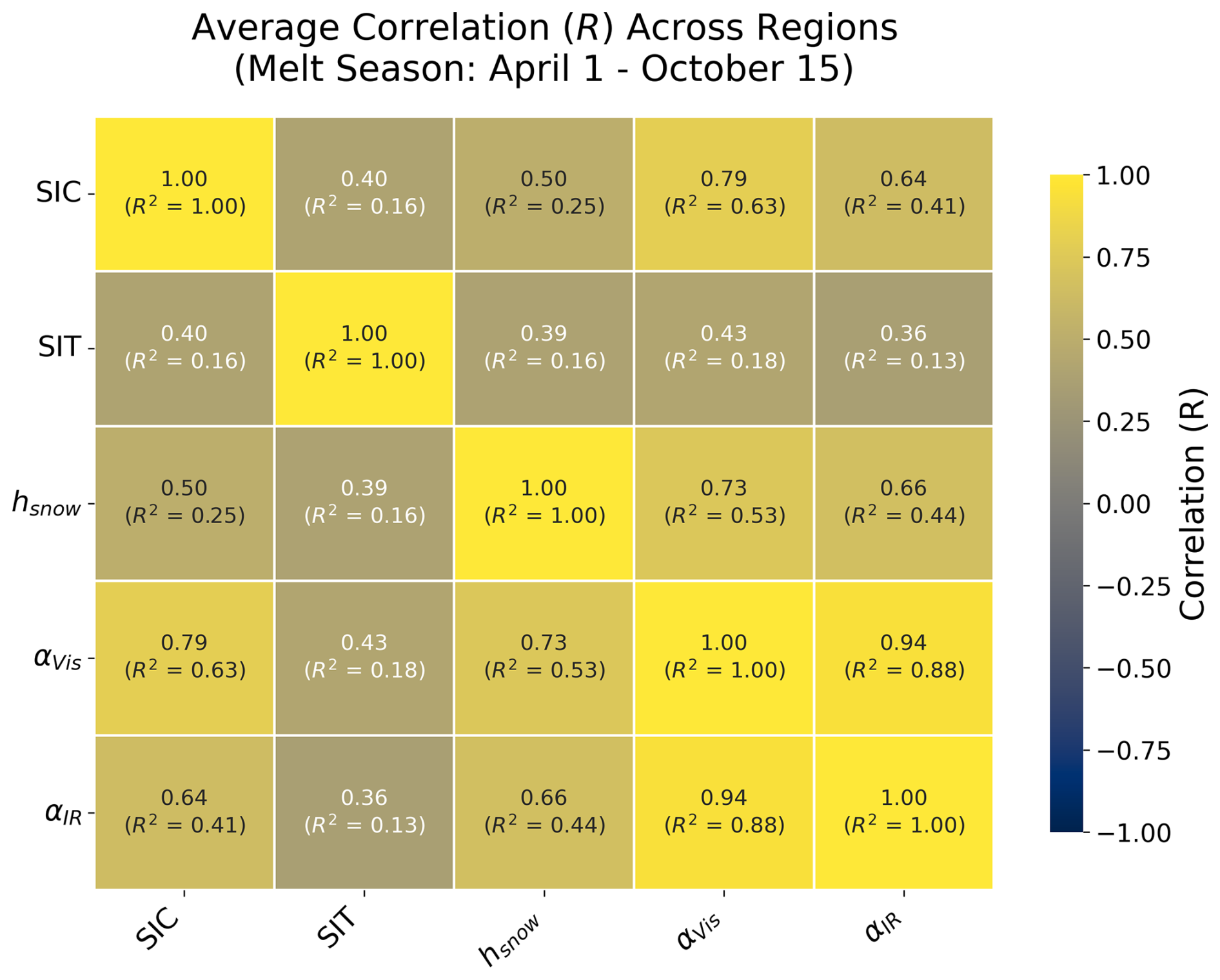
Figure 3 Correlation matrix (R) of Icepack main aggregate variables of interest averaged across all five regions specified in this study. Note that h_snow represents the snow depth averaged across the grid cell.

Due to the high correlation among the narrow-band components of SIAL in Icepack, we have consolidated these components into a single broadband SIAL for analysis. This simplification enables direct comparison of SIAL with SIC and SIT without reducing the overall complexity of the SIAL output. While all four narrow-band components are assimilated within the DA framework, our analysis focuses on this derived broadband component of the model output, defined as

$$\begin{array}{}\text{(3)}& \begin{array}{rl}{\mathit{\alpha }}_{\mathrm{broadband}}\left(\mathrm{SIAL}\right)& =\left(\mathrm{0.00318}\times {\mathit{\alpha }}_{\mathrm{DirVis}}+\mathrm{0.00182}\times {\mathit{\alpha }}_{\mathrm{DirIR}}\right.\\ & \left.+\mathrm{0.63282}\times {\mathit{\alpha }}_{\mathrm{IndVis}}+\mathrm{0.36218}\times {\mathit{\alpha }}_{\mathrm{IndIR}}\right).\end{array}\end{array}$$

From this point on, all references to “SIAL” refer to the broadband albedo component. The weighting for each of the broadband components is provided in the CICE Consortium (2025).

4 Results

4.1 RMSE Calculation and Statistical Significance

We calculate the ensemble mean (μ) RMSEs for SIC and SIT relative to eleven distinct TRUTH simulations, each based on a different randomly selected ensemble TRUTH member, for multiple assimilation experiments: SIAL-only (at low, medium, and high uncertainty levels; see the Methods section), SIC-only, SIT-only, SIC and SIT, all-variable assimilation (with low SIAL uncertainty), and a control free-run (Fig. 4). Error bars represent 95 % confidence intervals around the mean RMSE, calculated across 11 TRUTH simulations (ensemble members 3, 5, 8, 10, 12, 14, 16, 19, 21, 25, and 28) using bootstrap resampling.

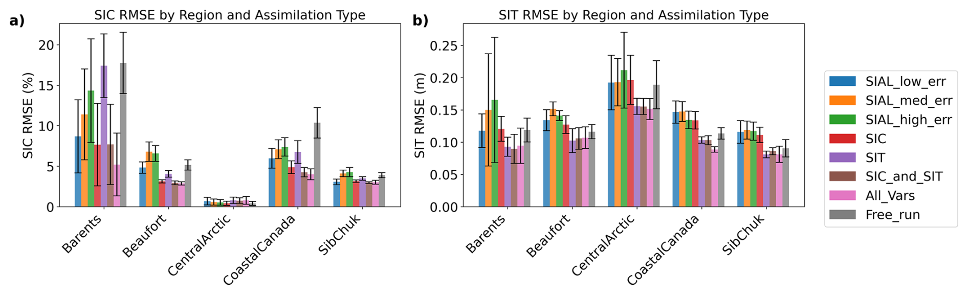
Figure 4 Panels (a) and (b) show the ensemble mean RMSEs relative to the TRUTH for 2011 SIC and SIT, respectively, across five key Arctic regions (Barents Sea, Beaufort Sea, Central Arctic, Coastal Canada, and Siberian-Chukchi Sea), averaged over 11 TRUTH simulations. Error bars represent 95 % confidence intervals computed via bootstrap resampling across the 11 TRUTH cases.

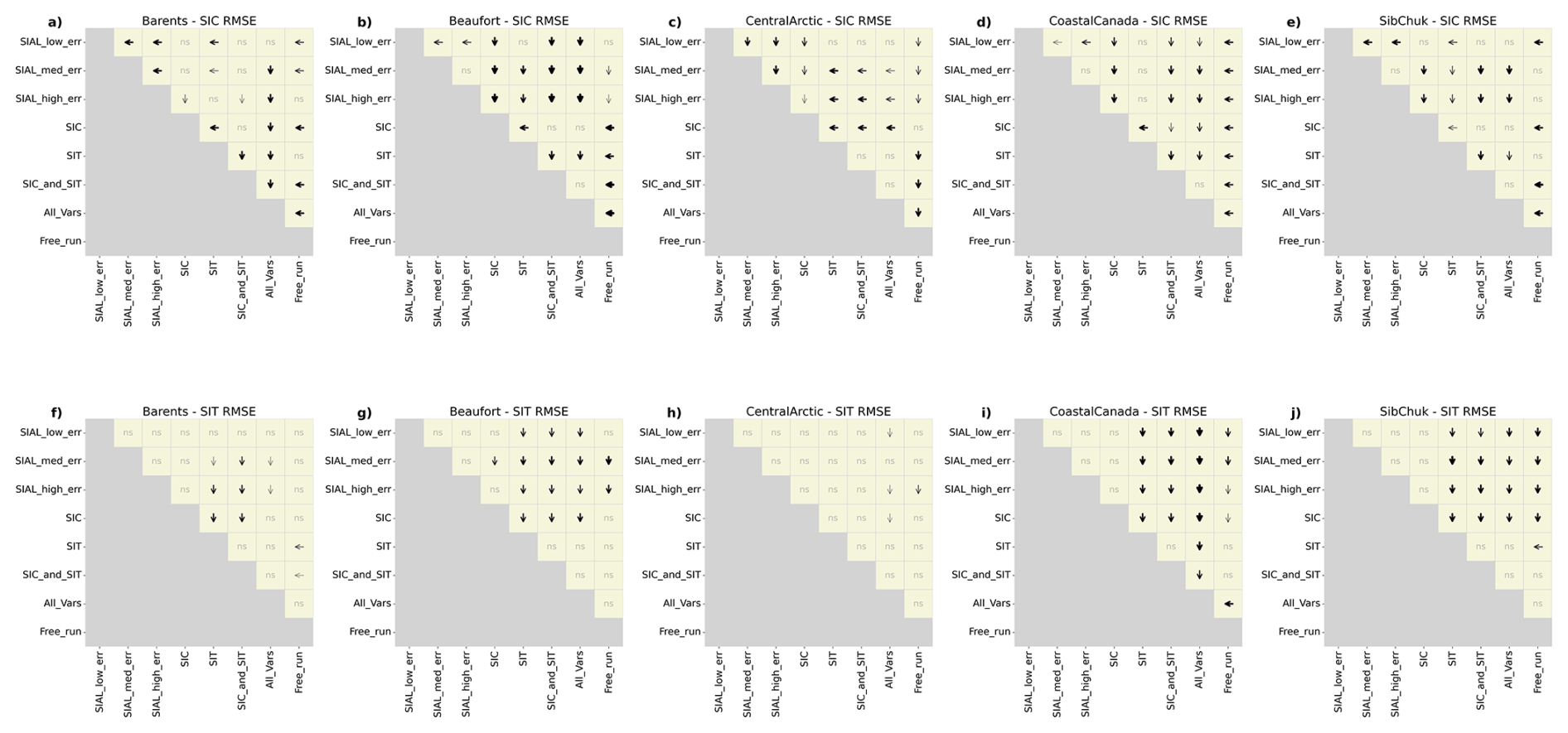
Figure 5 Pairwise statistical comparison of RMSEs (relative to the TRUTH) for different assimilation experiments across five regions for SIC (a–e) and SIT (f–j). Arrows indicate statistically significant differences (p<0.05), pointing toward the assimilation experiment with lower RMSE; arrow thickness increases with statistical confidence (smaller p-values). The label “ns” denotes non-significant comparisons. For example, in the top left tan square of panel (a), the arrow points from medium-uncertainty SIAL assimilation toward low-uncertainty SIAL assimilation in the Barents Sea, indicating that the latter achieves significantly lower SIC RMSE relative to the TRUTH. Assimilation cases include SIAL (low, medium, and high uncertainty), SIC, SIT, SIC and SIT, all variables (with medium SIAL uncertainty), and a free-run control. Exact p-values are provided in Table S1.

Figure 5 summarizes which 2011 assimilation experiments result in significantly different RMSE (relative to the TRUTH) outcomes (p<0.05), grouped by region and RMSE type (SIC or SIT). For each pair of experiments, we first apply the Shapiro–Wilk test to assess the normality of the RMSE distributions. If both distributions are approximately normal, we use Welch's t-test; otherwise, we employ the non-parametric paired Wilcoxon test. In the upper triangular matrix of each panel, arrows denote statistically significant differences, pointing from the higher to the lower mean RMSE relative to the TRUTH. Arrow thickness reflects the strength of the statistical evidence, with thicker arrows corresponding to smaller p-values. Comparisons that do not meet the significance threshold are labeled as “ns” (not significant). We provide the full set of p-values in Table S1. We obtain similar results when analyzing other free-run years, suggesting that the findings are not year-specific (not shown).

The statistical significances of differences in RMSE (relative to the TRUTH) vary substantially by region (Fig. 5). We observe the largest RMSE improvements relative to the TRUTH within the Barents Sea region. In particular, there is no statistically significant difference in SIC RMSE between assimilating only SIAL (with low observational uncertainty) and assimilating all variables. However, this equivalence breaks down when the SIAL observational uncertainty increases; there assimilating all variables performs significantly better. SIAL assimilation – under both low and medium uncertainty – performs similarly to SIC assimilation. However, SIC-only assimilation performs significantly worse than all-variable assimilation. For low and medium uncertainty, SIAL assimilation also outperforms SIT assimilation and the free run in terms of SIC RMSE (Fig. 5a). If SIAL uncertainty is constrained to low uncertainty it performs on par with SIT assimilation in terms of SIT RMSE (Fig. 5f). Assimilating SIT-only or SIC-and-SIT led to the only reductions when compared to the free run of SIT RMSE in the Barents region. We attribute the relatively large impact of DA to the initial model spread in the Barents region (Fig. 2).

In the Beaufort Sea, assimilating SIAL actually degrades performance relative to the free run when the observational uncertainty is not constrained to low values. This indicates that SIAL assimilation is not beneficial in this region. Assimilating SIC, on the other hand, leads to reductions in SIC RMSE, while for SIT RMSE no experiment performs significantly better than the free run. The model configuration for ice in this region is very rigid; as shown in Fig. 2, the simulated ice transitions from 100 % to 0 % SIC within roughly 3–5 d (depending on the year), with extremely limited ensemble spread. This behavior is likely a consequence of disabling ice deformation to represent landfast ice, which suppresses dynamical adjustments and limits ensemble variability.

Because SIAL inherently decreases during snowmelt and melt-pond formation, assimilating SIAL pushes Icepack toward an ice-free state earlier than the TRUTH, contributing to the degraded performance. Further research into ensemble generation for landfast ice and model–observation consistency is needed to clarify how SIAL and SIC should covary under these conditions. Finally, the chosen location may lie outside the region of strictly landfast ice within the Beaufort Sea, meaning that fully disabling ice dynamics by zeroing the closing file may not be appropriate for this site.

In the Central Arctic, an interesting pattern emerges: for SIC RMSE, no experiment with assimilation outperforms the free run, and in fact every variable-assimilation experiment except SIC-only assimilation performs worse than the free run. This behavior likely stems from the very low model spread in this region (Fig. 2), where SIC is tightly constrained and the assimilation increments push the model outside the limited ensemble envelope.

Similarly, few statistically significant differences appear in SIT RMSE within the Central Arctic (Fig. 5h). No experiment – including SIT-only assimilation – significantly outperforms the free run. The large SIT RMSE reflects the challenge of accurately representing thick, multi-year ice in the model, and is further exacerbated in SIT-assimilation experiments by our prescribed SIT observational uncertainty, which scales linearly with ice thickness (Table 1). Nonetheless, SIT assimilation does tend to reduce SIT RMSE on average (Fig. 4b), even if the improvement is not statistically significant.

In the Coastal Canada region, SIAL assimilation – regardless of observational uncertainty or assimilation type – significantly outperforms the free run in terms of SIC RMSE. Assimilating SIC and SIT together performs statistically as well as assimilating all variables for SIC RMSE. For SIT RMSE, however, all-variable assimilation performs significantly better than SIC-and-SIT assimilation. Notably, both SIAL assimilation (at all uncertainty levels) and SIC-only assimilation lead to higher SIT RMSEs relative to the TRUTH. In fact, only all-variable assimilation shows a statistically significant improvement over the free run for SIT RMSE.

Despite the benefits of SIAL assimilation in the Barents and Coastal Canada regions, results in the Siberian–Chukchi Sea are more nuanced. For SIC RMSE relative to the TRUTH, the observational uncertainty associated with SIAL plays a critical role. Only SIAL assimilation with low observational uncertainty yields statistically significant improvements over both the free run and SIT-only assimilation. When SIAL uncertainty cannot be constrained to low values, SIC and SIT assimilation statistically outperform SIAL assimilation. This highlights the importance of accurately characterizing SIAL uncertainty to ensure robust and meaningful assimilation outcomes. For SIT RMSE, SIAL assimilation (regardless of uncertainty level) and SIC-only assimilation both degrade performance relative to the free run. SIT-only assimilation is the only configuration that statistically outperforms the free run in this region.

4.2 Percent Difference Metrics to Compare Assimilation Experiments

Figure 6 shows that the comparative value of all-variable assimilation (including SIAL assuming low uncertainty) relative to SIC-only, SIT-only, or SIC-and-SIT assimilation varies substantially across regions. Overall, all-variable assimilation tends to perform better – especially in regions with intermediate ice conditions. However, in the Central Arctic, assimilating all variables instead of SIC-only often results in worse SIC RMSE (red shading). This underscores the need to identify region-specific combinations of assimilated variables that optimize Arctic-wide performance through incremental DA adjustments across the ITD.

Figure 6 Percent RMSE differences between all-variable assimilation (with low SIAL uncertainty) and SIC-only, SIT-only, or SIC-and-SIT assimilation (columns, left to right) across Arctic regions. Rows are grouped by RMSE metric relative to the TRUTH: SIC RMSE (a–c) and SIT RMSE (d–f). Values are computed relative to the free-running control using Eq. (2). Each cell shows the difference between the percent RMSE reduction achieved by all-variable assimilation and that achieved by SIC, SIT, or SIC-and-SIT assimilation. Negative values (blue) indicate better performance by all-variable assimilation, while positive values (red) indicate worse performance. Darker shading indicates larger magnitude. Values are shown for each region and ensemble TRUTH member.

Figure 6 also provides insight into the internal consistency of each assimilation experiment across ensemble members. Within each panel, the horizontal arrangement of ensemble TRUTH members (along the x-axis) allows for direct comparison of RMSE outcomes under different regions. When a given row of a subplot (i.e., region) is dominated by a single color or shade, this indicates that the impact of adding SIAL assimilation relative to SIC and/or SIT assimilation is consistent across the ensemble. For example, the Barents and Coastal Canada regions exhibit predominantly blue shading for SIC RMSE, suggesting robust improvements from added SIAL assimilation relative to SIC and/or SIT assimilation across nearly all ensemble members. In contrast, rows with a mixture of red and blue shading – such as the Beaufort Sea and Central Arctic – reflect less agreement among ensemble members, implying greater sensitivity to initial conditions (e.g. limited model spread) or synthetic observational noise.

This spatial and ensemble-level agreement underscores the reliability of conclusions drawn from regions with consistent shading and highlights the importance of ensemble spread in evaluating assimilation performance. Notably, trends appear to be more consistent across regions for SIC RMSE than for SIT RMSE. This observation is consistent with results shown in Fig. 4, where all-variable assimilation sometimes increased the SIT RMSE spread, especially compared to SIC-and-SIT assimilation.

4.3 Uncovering Model Deficiencies via Category-Wise SIAL Assimilation in the Siberian–Chukchi Sea

From Fig. 5, it is evident that SIAL assimilation, when not constrained to a low observational uncertainty, performs poorly compared to other commonly assimilated sea ice variables for SIC RMSE within the Siberian-Chukchi Sea, even compared to the free run. To further investigate this potential discrepancy, we ran assimilation of category-specific SIAL observations in this region.

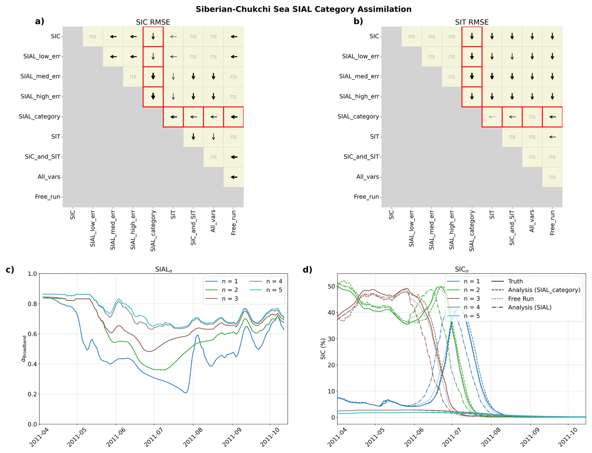
Figure 7 Siberian-Chukchi Sea results for the SIAL category-wise assimilation experiment. (a) Pairwise statistical significance of differences in mean RMSE for SIC among assimilation configurations. Black arrows indicate statistically significant differences in RMSE between assimilation configurations (p<0.05), pointing toward the experiment with lower RMSE relative to the TRUTH. “ns” denotes differences that are not statistically significant. Red boxes highlight comparisons between SIAL_category and all other assimilated variables and uncertainties. (b) As in panel (a) but for SIT RMSE. (c) Time series of domain-averaged broadband albedo (α_broadband) for eleven SIAL ensemble mean thickness category members (n=1 to 5). (d) Corresponding time series of mean SIC (%) for the same eleven ensemble members, including TRUTH, free run, and analysis under category members (n=1 to 5).

Figure 7 illustrates the impact of assimilating category-specific SIAL observations at the medium SIAL uncertainty level (±14 %). To represent uncertainty in broadband albedo as a function of ice thickness category, we applied a skewed uncertainty distribution in which thinner ice categories were assigned greater albedo uncertainty than thicker categories. This reflects the assumption that observational and modeling challenges in characterizing surface conditions (e.g., open water, melt ponds) are more prevalent over thin or newly formed ice (Nicolaus et al., 2012; Perovich et al., 2002). While this remains a broad approximation, the objective of this assimilation experiment is not to rigorously quantify category-wise SIAL uncertainty, but rather to diagnose potential deficiencies in the model's aggregate assimilation behavior.

Each thickness category was associated with a representative albedo range, and uncertainties were distributed using a physically informed, inverse-weighted scheme:

$$\begin{array}{}\text{(4)}& {\mathit{\sigma }}_n=\sqrt{\left({\displaystyle \frac{w_n\cdot {\mathit{\epsilon }}_{\mathrm{total}}}{\sum w_n}}\right)\cdot {\displaystyle \frac{(\mathrm{\Delta }{a}_n{)}^{\mathrm{2}}}{\mathrm{12}}}},\end{array}$$

where σ_n is the standard deviation of albedo assigned to the nth thickness category. Here, Δa_n denotes the width of the representative albedo interval for that category (i.e., the difference between the upper and lower albedo bounds of the bin), and a_n,right is the upper bound of that interval. The weight $w_n=\mathrm{1}/(a_{n,\mathrm{right}}+\mathrm{1})$ decreases as the upper bound increases, so thickness categories with lower maximum albedo (typically thinner ice or ponded ice) receive larger weights.

The total variance ε_total=0.14², is based on aggregate (medium) observational uncertainty across all ice types. Division by 12 assumes a uniform distribution of uncertainty within each albedo bin.

We note that the inverse weighting intentionally assigns greater absolute uncertainty to low-albedo, thin-ice categories (i.e., melt ponds and bare ice), reflecting the fact that these surfaces are generally more difficult to resolve with satellite retrievals due to their smaller scale and higher spatial variability. This scheme does not strictly match the 14 % medium relative uncertainty of aggregate SIAL observations, which would naturally assign smaller absolute errors to lower SIAL values. Rather, it represents a physically informed adjustment that concentrates uncertainty where retrievals are expected to be less reliable, while still ensuring that the total variance across all categories equals the reported ε_total.

Applying this category-specific assimilation results in significant improvements in reducing SIC and SIT RMSE within the Siberian-Chukchi Sea compared to most aggregate assimilation experiments. This methodology was also applied to other regions, but results there were largely insignificant except in other seasonal ice locations (e.g. Barents and Beaufort Seas), motivating a focused analysis on the Siberian-Chukchi region for this portion of the study. The top row of Fig. 7 demonstrates that assimilating SIAL by category – assuming the medium skewed uncertainty distribution described in Eq. (4) – outperformed all other assimilation strategies for SIC RMSE, including experiments that assimilated all aggregate variables. For SIT RMSE, SIAL by category assimilation also performed on par with, or better than, all other assimilation configurations.

What causes this significant RMSE improvement relative to the TRUTH that is missed in the aggregate synthetic observations? Figure 7c offers some insight. This plot shows the SIAL by category, averaged over eleven different ensemble TRUTH members. The thickness categories are indexed by n, where n=1 corresponds to the thinnest ice and n=5 to the thickest ice. Notably, SIAL evolves differently across categories: in particular, SIAL in the thinnest ice category (n=1) decreases rapidly in early April, while the remaining categories exhibit relatively stagnant behavior. This decoupled, category-specific SIAL trend occurs in the Siberian–Chukchi Sea due to the Icepack model configuration choice fluxing open water.

The prescribed SHEBA deformation promotes ridging and associated lead opening, whereby open water occupies the fractional area lost to ridging. In the Siberian–Chukchi Sea, ambient conditions are sufficiently cold for these leads to rapidly refreeze, resulting in the prevalence of thin ice (category n=1) with minimal snow cover. This dramatically reduces the SIAL in n=1, producing incorrect aggregate albedo estimates. Because the category time series (equivalent to Fig. 7c) in non-seasonal regions (i.e., the Central Arctic and Barents Sea) track a common signal, the aggregate SIAL in these regions closely follows the underlying category-level evolution. This helps explain why aggregate SIAL assimilation generally performs at least as well as the baseline (i.e., is not significantly worse) relative to the free run, even under higher observational uncertainty in these regions. There, the category distribution is either relatively stable or strongly weighted toward a single category. In the Central Arctic, thicker ice and a weaker seasonal cycle limit category exchange and maintain stability, whereas in the Barents Sea the distribution is dominated by a single category. In both the Central Arctic and Barents Sea, the aggregate SIAL closely follows the temporal evolution of the dominant category, helping explain why aggregate SIAL assimilation generally performs well or comparably in those areas – even under higher observational uncertainty. In contrast, within the Siberian–Chukchi Sea, Icepack does not evenly distribute the decrease in SIAL across thickness categories. This introduces significant deficiencies in aggregate assimilation when SIAL uncertainty is unconstrained. In effect, the aggregate SIAL diverges from the true category-level dynamics, leading to an improper DA adjustment of model state variables aice_n and vice_n. When uncertainty is high, this results in larger SIC and SIT RMSE relative to the TRUTH than even the free-running control simulation (see Figs. 4–5).

The issue originates within Icepack: SIC_n+1 and SIC_n have opposing changes, but SIAL_n+1 and SIAL_n both decrease so SIAL_n does not increase correspondingly to account for the influx of ice transitioning from thicker to thinner categories (see bottom row of Fig. 7). This SIAL adjustment is likely (at least partially) incorrect and influences the formation of melt ponds within the thermodynamics module. Recent developments in Icepack have aimed to improve melt pond parameterization; however, version 1.4.0 of Icepack does not support the new scheme. The authors have included information within the Supplement about utilizing different melt pond schemes available in Icepack version 1.4.0 to best represent the surface conditions during this study. We acknowledge that aggregate SIAL observations in the real world can further complicate Icepack DA discrepancies – SIAL_n may behave differently across categories in the model, and such a variation would not be accurately updated using a coarse aggregate SIAL observation.

5 Discussion

5.1 Potential Mechanisms for RMSE Reduction and Benefits of SIAL Assimilation

As highlighted above, incorporating SIAL as an additional assimilated variable represents a novel approach with numerous potential benefits for improving sea ice modeling. Currently, SIT is widely considered a robust assimilation variable due to its high sensitivity to physical processes, long memory, and predictive power. For instance, studies have shown that assimilating SIT (especially in winter) in models significantly enhances the accuracy of sea ice extent forecasts, underscoring its predictive value (Song et al., 2024; Ono et al., 2020; Williams et al., 2023). Our results further support this claim: when the uncertainty is tightly constrained (as assumed in this study), SIT assimilation is highly effective at reducing model biases, particularly for SIT RMSE. However, summertime SIT retrievals from CryoSat-2/SMOS and other sources are generally not considered reliable or used operationally, creating a gap in available observables and further underscoring the need to include SIAL as an assimilated variable as it is predominately available in summertime months (Edel et al., 2025; Riihelä et al., 2024).

We propose three mechanisms that may explain how real-world SIAL aggregate assimilation, when constrained to “low” observational uncertainty and performed concurrently with aggregate SIC and SIT assimilation, contributes to the widespread reductions in SIC and sometimes SIT RMSE (Fig. 6), which are directly linked to model state variables.

1. SIAL Observational Uncertainty vs. SIC and SIT Uncertainties. Relative to SIC and especially SIT, SIAL observational uncertainty is likely lower, particularly during the summer months. The known uncertainty for SIAL is between 0 %–14 % (Karlsson et al., 2023). In contrast, SIC known observational uncertainty is likely on the order of 5 %–10 % (Zhang et al., 2021; Peng et al., 2013), but higher in the MIZ and during the presence of melt ponds (Kern et al., 2016). SIT observational uncertainty varies, ranging from 10 %–100 % depending on ice thickness. Therefore, during summer months when the ice is thin, the observational uncertainty may approach or even exceed the SIT measurement (Song et al., 2024). Note that we assumed an optimistic SIT uncertainty of ±10 % in this study. The actual uncertainty is likely higher, especially when using older observational data such as from CryoSat-2 (Chen et al., 2024). Thus, for reanalysis datasets spanning the pre-ICESat-2 era (before 2019), SIAL may provide a stronger observational constraint than other sea ice variables. This suggests that SIAL assimilation during summer months may be particularly beneficial, as SIAL leads to more constrained sea ice simulations when SIT (and MIZ SIC) observations are particularly sparse and uncertain.

2. SIAL Assimilation as an Early Melt Onset Indicator. SIAL assimilation provides an early indication of melt onset, which can mitigate low adaptive inflation (i.e., the temporally varying adjustment of ensemble spread applied within the QCEFF to prevent underestimation of forecast uncertainty, see Sect. S1 of the Supplement) during the early melt season. This is observed in the Barents and Coastal Canada regions, where the addition of SIAL assimilation helps to prevent ensemble spread collapse and thus filter divergence. For example, in the Barents Sea, the mean incremental SIC changes in SIAL DA (with medium uncertainty) are substantially larger during the early melt season compared to those from SIT assimilation (and comparable to that of SIC DA), often resulting in improved agreement with the TRUTH member in early summer (Fig. A2). SIAL, acting as a proxy for snow cover and melt ponds, often exhibits a gradual decrease before SIC begins its rapid decline in the summer months. This early signal helps constrain the bounded assimilation of state variables aice_n and vice_n, effectively moderating inflation in the model during late summer. At the same time, however, this early SIAL decrease can lead to worsened DA performance when assimilating SIAL-only, as seen in the Beaufort Sea, when ensemble spread is insufficiently constrained (Fig. 4).

   Careful monitoring of the adaptive inflation scheme is crucial, as SIAL, SIC, and/or SIT assimilation may result in insufficient model spread, particularly when observations are assigned a low observational uncertainty. Xiong et al. (2002) emphasized the importance of balancing observational uncertainty assignments to avoid introducing excessive bias or overconfidence in assimilation outcomes. This balance is especially significant during the early melt season, where reduced spread from sea ice DA can impact the model's responsiveness to rapidly changing ice conditions. See the Supplement for additional detail about the adaptive inflation used in this study.

3. SIAL Provides Contextual Clues for Sea Ice Fractional Coverage. SIAL is a critical variable in understanding the fractional coverage of different surface types within a grid cell, such as snow-covered ice, bare ice, melt ponds, and open water. The assimilation of SIAL provides continuous insights into the energy balance of the sea ice surface, which is essential for accurately predicting seasonal changes in sea ice extent and thickness. Springtime melt ponds, for instance, are strong indicators of the September sea ice minimum (Schröder et al., 2014). Snow cover and late-season snowfall also influence SIAL and, consequently, the rate of ice melt (Chapman-Dutton and Webster, 2024; Vérin et al., 2022; Perovich et al., 2017).

   In Icepack, SIAL can be expressed as a weighted sum of the contributions from snow, melting ice, bare ice surfaces, and open water:

   $$\begin{array}{}\text{(5)}& \begin{array}{rl}{\mathit{\alpha }}_{\mathrm{broadband}}& =f_{\mathrm{snow}}{\mathit{\alpha }}_{\mathrm{snow}}(T,\mathrm{age})\\ & +f_{\mathrm{melt}}{\mathit{\alpha }}_{\mathrm{melt}}(T,h_{\mathrm{melt}})\\ & +f_{\mathrm{ice}}{\mathit{\alpha }}_{\mathrm{ice}}(T,h_{\mathrm{ice}})\\ & +f_{\mathrm{openwater}}{\mathit{\alpha }}_{\mathrm{openwater}}\end{array}\end{array}$$

   where:

   • f_snow, f_melt, f_ice, and f_openwater are the fractional area weights for snow-covered ice, melt ponds, bare ice, and open water, respectively,

   • α_snow, α_melt, α_ice, and α_openwater are the albedo values for each surface type,

   • T represents temperature,

   • age is the snow age,

   • h_melt and h_ice are the melt pond depth and ice thickness, respectively.

   This formulation highlights how SIAL serves as a diagnostic variable that encapsulates the physical processes driving seasonal surface transitions in the Arctic. As we have seen from our results, by also assimilating SIAL, the model is better equipped to constrain observed variables like SIC and SIT, as SIAL (aggregate) acts as an integrative measure of surface state changes during the melt season. This contextual information has been shown above to help reduce biases and improve forecasts of Arctic sea ice behavior when assimilated together with SIC and SIT.

SIAL is more than a simple proxy for fractional coverage; it encapsulates key information about the radiative and thermodynamic state of the sea ice surface. By capturing both spatial and spectral variations in ice and snow reflectivity, SIAL helps constrain the energy balance of the ice–ocean–atmosphere system and offers insight into melt processes, pond evolution, and snow metamorphism. This richness of information allows SIAL to provide a form of memory for the ice system – similar to ice age, which has been shown to be a robust indicator of sea ice state (Zhang et al., 2018). However, unlike ice age, which may lose relevance as the Arctic transitions to a primarily first-year ice regime (Sumata et al., 2023; Meier et al., 2023), SIAL is expected to remain an important variable. Its demonstrated utility in highly seasonal regions like the marginal ice zone (e.g., Barents Sea) underscores its value, and its importance may further grow as Arctic precipitation shifts from snow to rain (McCrystall et al., 2021), altering surface albedo and melt dynamics in ways that SIAL can continue to capture.

6 Conclusions

The results of this study suggest that SIAL assimilation is a robust addition to assimilating traditional sea ice variables, such as SIC and SIT. The addition of SIAL assimilation performs well due to SIAL's relatively low observational uncertainty, its ability to better predict the melt onset, and its intrinsic relationship to snow, bare ice, and melt pond fractional coverage. In this one-dimensional Icepack experiment, the addition of SIAL assimilation to SIC and SIT assimilation performs on par with or significantly better than SIC and SIT assimilation.

We acknowledge that this study was conducted in a one-dimensional idealized environment and emphasize the need for further experimentation using a fully coupled global climate model to comprehensively assess the impact of SIAL assimilation on the mean sea ice state in a multi-dimensional framework. In particular, future research should investigate the performance of satellite-derived SIAL assimilation within a three-dimensional sea ice model to better quantify the advantages and limitations identified in this study.

A key challenge is the limited understanding and quantification of uncertainties associated with satellite SIAL retrievals. This remains an underexplored area, and our study encountered difficulties in establishing a consensus on how best to represent these uncertainties. The development of additional airborne field campaigns that better capture the aggregate satellite spatial scale would support more robust cross-validation of satellite products.

Despite these challenges, we remain optimistic about the potential of SIAL assimilation, particularly given the extensive availability of high-resolution satellite SIAL products spanning the satellite era. Notably, the CLARA-A3 surface albedo product, produced by EUMETSAT, provides pentad SIAL estimates at 25 km resolution on the Equal-Area Scalable Earth (EASE) grid across multiple narrow-band frameworks (see video supplement). Similarly, APP-x, developed in collaboration with NOAA and the University of Wisconsin, offers twice-daily narrow- and broadband SIAL composites at the same resolution (see video supplement). These observational datasets offer a promising addition to conventional SIC and SIT assimilation approaches and hold considerable potential for improving sea ice reconstruction over the satellite observational period (1979–present). Continued investigation of these products and their incorporation into advanced data assimilation systems is critical for unlocking their full potential.

Appendix A

Supplementary figures supporting the main analysis are provided below (Figs. A1–A2).

Figure A1 Observational uncertainty distributions for SIC (a), SIT (b), and SIAL (c). Floors in uncertainty are included to prevent zero uncertainty at the variable bounds. Note that there are three different uncertainty scenarios for SIAL to account for unknowns in SIAL retrieval estimates. The normalized amount of uncertainty by variable (0–1) is included in the bottom-right (d) for comparison.

Figure A2 Mean magnitude of DA increments in SIC, expressed as absolute percent change from the prior state, averaged across 11 assimilation experiments. Each panel corresponds to a different assimilation configuration: SIAL (a; medium uncertainty), SIC (b), and SIT (c). Data are smoothed using a 7 d rolling average. Regions with rare high-magnitude increments (≥ 6 %) are annotated with their maximum value for clarity. Notably, the SIAL DA configuration shows pronounced early-season activity, particularly in the Barents Sea region, while late-season peaks in Coastal Canada are prominent in all configurations.