Greenland Monthly Accumulation Maps (1960–2022): A Statistical Semi-Empirical Bias-Adjustment Model

Accurate estimates of snow accumulation over the Greenland ice-sheet are essential for reliable projections of sea-level rise. These are typically obtained from regional climate models, which carry systematic temporal and spatially variable biases, contributing to substantial uncertainties in sea-level rise projections. Here we present a novel statistical-semi-empirical model for bias-correcting gridded accumulation output from any regional climate model or reanalysis product, utilising the SUMup dataset, which provides the most comprehensive spatial and temporal coverage of surface mass balance observations to date. The method employs Empirical Orthogonal Function analysis to decompose the model accumulation output into the dominant patterns of spatial variability and their temporal evolution. Adjustment coefficients derived by fitting SUMup data enable the reconstruction of spatially complete, bias-corrected accumulation fields.

We apply this approach to monthly accumulation output from the HIRLAM–ECHAM Regional Climate Model (HIRHAM5; 1960–2022), the Modèle Atmosphérique Régional (MAR3.14; 1960–2022), the Regional Atmospheric Climate Model (RACMO 2.4p1; 1980–2022), and the Copernicus Arctic Regional Reanalysis (CARRA; 1991–2022). Initial mean point-wise biases of −7.4 % (HIRHAM), −0.5 % (MAR), 0.0 % (RACMO) and +10.1 % (CARRA) (1991–2022), statistically significant for all models except RACMO, are reduced to ± 0.3 % following adjustment. Resulting bias-corrected mean annual accumulation rates over the ice sheet are estimated at 469 mm yr⁻¹ (HIRHAM), 412 mm yr⁻¹ (MAR), 435 mm yr⁻¹ (RACMO) and 408 mm yr⁻¹ (CARRA) between 1991–2022. Inter-model agreement improves significantly in the observation-rich accumulation zone, with a 68 % reduction in standard deviation of mean accumulation estimates, but deteriorates by 27 % in the sparsely sampled ablation zone, highlighting the need for additional observational constraints. Model bias is dominated by the southern ice sheet, with the largest statistically significant contributions from the south-east for HIRHAM (−39 to −54 Gt yr⁻¹) and MAR (+30 to +33 Gt yr⁻¹), and the south-west for RACMO (+20 to +26 Gt yr⁻¹) and CARRA (+34 Gt yr⁻¹). Temporal trends and temperature sensitivities exhibit a pronounced east-west contrast, with the east dominated by strong positive responses and negative responses in the west.

The framework outlined in this study offers a scalable, transferable solution to improve accumulation estimates through enhanced integration of observational data, providing an improved input to ice-sheet models, with the potential to reduce uncertainties in future sea-level rise projections.

1 Introduction

The Greenland Ice Sheet (GrIS) has become the greatest single cryospheric contributor to present-day global sea-level rise (Chen et al., 2017; van den Broeke et al., 2017, 2016), accounting for ∼ 22 % of the ∼ 3.3 mm yr⁻¹ total mean sea-level rise between 2002 to 2022 (Hanna et al., 2024; Jia et al., 2022). Since the mid 1990s, mass loss from the GrIS has been driven by changes in Surface Mass Balance (SMB) (Hofer et al., 2020; van den Broeke et al., 2016, 2009), overtaking ice loss from calving. SMB is defined as the mass accumulated through precipitation, minus the mass lost through meltwater runoff, sublimation, evaporation, and wind redistribution. As the only net mass input, accumulation is crucial to constrain for accurate modelling of ice-sheet evolution. However, due to the complexity of processes governing precipitation, coupled with limitations in model resolution and simplified cloud microphysics, accumulation over the GrIS remains poorly constrained by models. As a result, regional climate models (RCMs) often fail to adequately capture this variability, leading to biased estimations of ice loss (Ryan et al., 2020) and substantial discrepancies between climate model projections (Otosaka et al., 2023).

The first studies investigating snow accumulation in the early 20th century established techniques such as stake measurements, snow pits, and shallow cores to deduce accumulation from snow height and seasonal layering. In the late 1950s, ice core projects analysing stable oxygen-isotope ratios provided new insights into past climate, leading to their systematic use in detailed accumulation studies (e.g. Box et al., 2013, 2009; Buchardt et al., 2012; Mosley-Thompson et al., 2001; Clausen et al., 1988). The introduction of ice-penetrating radar systems in the mid-1960s to track reflections from ice layers revealed that internal stratigraphy formed by seasonal snowfall could be used to infer accumulation rates, enabling continuous mapping of accumulation variability over vast regions (Robin et al., 1969). This laid the foundation for further ground-based radar surveys (Hawley et al., 2014; Miège et al., 2013; Medley et al., 2013), as well as airborne campaigns (Montgomery et al., 2020; Lewis et al., 2017; Koenig et al., 2016), greatly expanding coverage beyond areas accessible to in situ measurements.

One of the earliest comprehensive efforts to synthesise diverse observational data to map accumulation across the GrIS was by Ohmura and Reeh (1991). Using spatial interpolation of ice core, snow pit and coastal weather station data, they estimated mean accumulation to be 310 mm w.e., and provided one of the most accurate maps of GrIS accumulation at the time. This study was instrumental in advancing understanding of how topography and atmospheric circulation influence regional snowfall and ice sheet mass balance. Subsequent studies incorporated additional data with improved interpolation techniques (Cogley, 2004; Calanca et al., 2000; Ohmura et al., 1999), and enhanced understanding of regional variability (McConnell et al., 2001).

RCMs provided a way to estimate accumulation on spatially complete high resolution grids (Ettema et al., 2009; Fettweis et al., 2008; Box et al., 2006, 2004; Box, 2005). Similarly, climate reanalyses provided gridded accumulation fields (Hanna et al., 2008, 2006, 2005), with the advantage of assimilating satellite and in situ observations, such as atmospheric pressure and temperature (Simmons and Gibson, 2000). Reanalysis products could also serve as boundary conditions for RCMs, alongside ancillary weather station and remote-sensing observations. However, both RCMs and reanalyses inherently carry biases arising from coarse resolution failing to resolve complex terrain, simplified cloud microphysics, and sparse observational constraints.

To address model bias, Box et al. (2006) calibrated accumulation output from the Fifth Generation Mesoscale Model for polar climates (Polar MM5) using snow pit observations, identifying and correcting for systematic errors. Expanding on these advances, Burgess et al. (2010) combined firn core measurements and meteorological station precipitation data with high-resolution Polar MM5 output to create a spatially complete reconstruction of Greenland Ice Sheet accumulation. This hybrid methodology resolved inconsistencies in earlier studies that relied on sparse datasets or models alone, providing a new accumulation grid with enhanced regional accuracy. Using spatial interpolation of linear correction functions derived by region, Burgess found a mean snow accumulation rate of 337 ± 48 mm yr⁻¹, 16 %–21 % higher than previous estimates by Ohmura et al. (1999), Calanca et al. (2000) and Cogley (2004). This increase was primarily attributed to better representation of higher orographic precipitation provided by the hybrid approach, affecting the south-east in particular – a region with limited ice core coverage. Accumulation rates in the south-east were found to exceed 2000 mm yr⁻¹ and dominate inter-annual variability. Representing 31 % of the total accumulation, this region was found to have a substantial impact on ice-sheet SMB as a whole.

Providing one of the first spatially complete reconstructions of accumulation, Burgess et al. (2010) remains a cornerstone for understanding Greenland’s climate-driven ice loss. Numerous studies have since continued to improve on this foundation through incorporating new observations and enhanced model simulations (Mouginot et al., 2019; Sandberg Sørensen et al., 2018; van den Broeke et al., 2016; Khan et al., 2015; Velicogna et al., 2014; Box et al., 2013; Shepherd et al., 2012). Despite these advances, accumulation remains a major source of uncertainty in sea-level rise projections (van den Broeke et al., 2009).

Ice sheet models, and hence sea-level rise projections, require spatially complete gridded accumulation maps and are thus typically obtained from RCMs. RCMs are often validated using a combination of remote sensing products and in situ point observations from weather stations and firn cores. Although remote sensing technology can provide snowfall estimates, the accuracy of retrievals is restricted by challenges in sampling limitations and ground clutter (Ryan et al., 2020; Bennartz et al., 2019). Combined with the sparse distribution of weather stations and firn cores leaving vast regions without in situ coverage, RCM accumulation maps still carry significant uncertainties today (Ryan et al., 2020; Vernon et al., 2013). Though ice core, radar, snow pit and stake measurements can fill some in situ data gaps, point-to-pixel differences and challenges in aligning inconsistent temporal resolutions mean that the full range of available data remains under-utilised in systematic RCM validation.

Here we present a flexible statistical-semi-empirical model designed to utilise the full range of available in situ data to bias-adjust any gridded model accumulation output. This study advances prior work through leveraging the SUMup SMB dataset (Vandecrux et al., 2024), providing the most comprehensive basis for model correction to date. Using this diverse compilation of in situ observations derived primarily from ice-cores, airborne and ground-based radar, snow pits, stake measurements and automated weather stations, we produce spatially complete monthly bias-adjusted accumulation maps. While previous studies have used techniques such as universal kriging (Ohmura and Reeh, 1991), triangulated irregular networks (Burgess et al., 2010) and least-squares regressions (Box et al., 2013) to estimate or correct model bias with point-based observations, these approaches typically do not explicitly account for patterns of both spatial and temporal bias variability.

We base our method on Empirical Orthogonal Function (EOF) decomposition of the model accumulation output, which reveals the dominant patterns of spatial and temporal variability. Utilising robust least-squares optimisation, we fit each component of the decomposition to SUMup observations to derive a set of coefficients which adjust each component of the decomposition. This approach enables targeted correction of the model's spatial and temporal structure.

The aim of this study is to present a flexible bias-correction model for improving estimates of GrIS accumulation, which offers the potential to improve GrIS SMB estimates and downstream modelling of sea-level rise. We first present four model products to which the bias-adjustment is applied: the HIRLAM–ECHAM Regional Climate Model (HIRHAM) version 5, the Modèle Atmosphérique Régional (MAR) version 3.14, the Polar Regional Atmospheric Climate Model (RACMO) version 2.4p1, and the Copernicus Arctic Regional Reanalysis (CARRA), followed by an overview of the SUMup dataset and key data considerations. We then provide a detailed outline of the bias-adjustment method. Results are subsequently analysed in terms of mean and seasonal biases before and after bias-adjustment, and we examine the impact on long-term accumulation trends and temperature sensitivity. Lastly, we discuss the implications and limitations of these findings.

2 Data

2.1 Gridded Model Accumulation

We present bias-corrected accumulation maps for four models, including three RCMs and one reanalysis product: (1) the HIRLAM–ECHAM Regional Climate Model (HIRHAM) version 5 (Langen et al., 2017), (2) the Modèle Atmosphérique Régional (MAR) version 3.14 (Fettweis et al., 2020), (3) the Polar Regional Atmospheric Climate Model (RACMO) version 2.4p1 (van Dalum et al., 2024), and (4) the Copernicus Arctic Regional Reanalysis (CARRA) dataset (Schyberg et al., 2020). All models are forced with ERA5 (Hersbach et al., 2020) at their lateral boundaries, which provides atmospheric fields of temperature, humidity, wind and surface pressure. As none of the models are coupled with an ice-sheet model, ice extent and topography remain fixed. Accumulation output is obtained at monthly resolution and is approximated using SMB components excluding runoff. The implications of this approximation relative to SUMup observations are discussed in section 2.3.

2.1.1 HIRHAM5 Regional Climate Model (1960–2022, 5.5 km)

HIRHAM5 (Christensen et al., 2017) is the fifth generation of the HIRHLAM-ECHAM regional climate model, which combines the dynamics of the HIRLAM model (Undén et al., 2002) with the physical parametrisation schemes of the ECHAM model (Roeckner et al., 2003). Over the Greenland domain, HIRHAM5 is run on a rotated latitude–longitude grid with ∼ 5.5 km resolution, using 31 atmospheric levels and a time step of 90 s Langen et al. (2017). The model is 6-hourly forced at its lateral boundaries by ERA5 reanalysis (Hersbach et al., 2020), with ERA5 sea surface temperatures and sea-ice concentrations prescribed at the lower boundary. HIRHAM5 has been extensively evaluated against observations over Greenland (Langen et al., 2017, 2015; Lucas-Picher et al., 2012).

In HIRHAM, SMB is parametrised as:

$$\begin{array}{}\text{(1)}& {\mathrm{SMB}}_{\text{HIRHAM}}=P-E-\mathrm{RU},\end{array}$$

where P is the total precipitation, E, is evaporation including sublimation, and RU is surface meltwater runoff. Excluding runoff, we define accumulation as:

$$\begin{array}{}\text{(2)}& {\mathbf{Acc}}_{\text{HIRHAM}}=P-E.\end{array}$$

2.1.2 MARv3.14 Regional Climate Model (1960–2022, 5 km)

The Modèle Atmosphérique Régional (MAR) version 3.14 (Fettweis and Grailet, 2024) couples an atmospheric module Gallée and Schayes (1994) to Soil Ice Snow Vegetation Atmosphere Transfer (SISVAT) scheme (Ridder and Schayes, 1997), including a snow model based on CROCUS (Brun et al., 1992). The snow module resolves the dominant physical processes governing snowpack evolution, including thermal stratification, densification, meltwater percolation, grain size and snow drift. The model is laterally forced by ERA5 in 6 h intervals, which also provides sea surface temperatures and sea ice cover over ocean grid cells (Haacker et al., 2024). The model configuration has been calibrated over the GrIS (Fettweis et al., 2020) and extensively validated, showing improved agreement with in situ atmospheric measurements (Delhasse et al., 2020), remote sensing derived melt extent (Fettweis et al., 2011) and SMB observations (Fettweis et al., 2020), compared to earlier versions.

For MAR, SMB is parametrised as:

$$\begin{array}{}\text{(3)}& {\mathrm{SMB}}_{\text{MAR}}=P-\mathrm{SU}-\mathrm{SW}-\mathrm{RU},\end{array}$$

where P is total precipitation, SU is sublimation from snow/soil, SW is surface water and RU is surface meltwater runoff. Excluding runoff, accumulation is defined here as:

$$\begin{array}{}\text{(4)}& {\mathbf{Acc}}_{\text{MAR}}=P-\mathrm{SU}-\mathrm{SW}.\end{array}$$

2.1.3 RACMO2.4p1 Regional Climate Model (1980–2022, 11 km)

RACMO 2.4p1 (van Dalum et al., 2024), is a hydrostatic model that integrates the atmospheric dynamics of HIRLAM version 5.0.3 (Undén et al., 2002) with the physical parametrisations of the ECMWF Integrated Forecasting System. At the lateral boundaries, RACMO2.4p1 is forced by ERA5 reanalysis fields at 3-hourly intervals, including wind, temperature, humidity, and surface pressure, with sea surface temperature and sea-ice concentration also prescribed from ERA5. The polar version of RACMO includes specialised parameterisations for glaciated surfaces and polar boundary-layer processes, with a dedicated ice-sheet surface tile and a multilayer snow model that resolves snow metamorphism, compaction, melt, refreezing, and drifting-snow processes (Noël et al., 2018; Ettema et al., 2010). The simulations used here are taken from the R24 experiment on a pan-Arctic domain following the Arctic CORDEX standard, with ∼ 11 km horizontal grid spacing and 40 atmospheric layers.

RACMO2.4p1 shows generally good agreement with observations over Greenland, with improved representation of cloud microphysics, precipitation, and surface mass balance compared to the previous version (R23p3) (van Dalum et al., 2024).

In RACMO2.4p1, SMB is parametrised as:

$$\begin{array}{}\text{(5)}& {\mathrm{SMB}}_{\text{RACMO}}=P-\mathrm{SU}-\mathrm{ER}-\mathrm{RU},\end{array}$$

where P is precipitation, SU is sublimation including surface sublimation and sublimation of wind blown snow, ER is drifting snow erosion and RU is surface meltwater runoff (van Dalum et al., 2024). Excluding runoff, we define accumulation as:

$$\begin{array}{}\text{(6)}& {\mathbf{Acc}}_{\text{RACMO}}=P-\mathrm{SU}-\mathrm{ER}.\end{array}$$

2.1.4 CARRA Reanalysis (1991–2022, 2.5 km)

The CARRA reanalysis dataset (Schyberg et al., 2020) is built on the weather forecast model HARMONIE, standing for HIRLAM–ALADIN Research on Mesoscale Operational NWP in Euromed, which integrates developments from HIRLAM (High Resolution Limited Area Model) and ALADIN (Aire Limitée Adaptation Dynamique Développement International) (Bengtsson et al., 2017). CARRA is laterally forced by ERA5 reanalysis (Hersbach et al., 2020) and applies three-dimensional variational (3D-Var) data assimilation to incorporate multiple datasets (Schyberg et al., 2020), including, in Greenland, remotely sensed surface albedo (Kokhanovsky et al., 2023) and temperature, humidity, and wind speed measured by on-ice weather stations (Fausto et al., 2021; Vandecrux et al., 2023). With 2.5 km horizontal resolution and an improved representation of cold surfaces (Yang et al., 2020), CARRA agrees substantially better with in situ observations than ERA5 (Køltzow et al., 2022). It has been used to investigate recent warming over the Barents Sea (Isaksen et al., 2022), Arctic sea ice (Batrak et al., 2024) and increased glacier melt in Svalbard (Schmidt et al., 2023).

In CARRA, as a dedicated SMB variable is not available, we define accumulation as:

$$\begin{array}{}\text{(7)}& {\mathbf{Acc}}_{\text{CARRA}}=P-E-\mathrm{SU},\end{array}$$

where P is the total precipitation, E is evaporation, and SU is the time integrated snow evaporation flux. Monthly data is obtained by subtracting the 30 and 6 h daily forecasts and resampling to monthly sums.

2.2 Analysis Domain

We perform the bias-adjustment across the entire ice-sheet, defining a common ice mask derived from the PROMICE-2022 Ice Mask (Luetzenburg et al., 2025). This product provides a high-resolution delineation of the Greenland Ice Sheet and interior nunataks, encompassing a glacierised area of 1 725 648 km². Mapped from August 2022 Sentinel-2 imagery, it captures the GrIS margin with greater than 20 m horizontal accuracy, offering the most up-to-date and internally consistent representation of the GrIS extent currently available. Drainage basin boundaries used are also adopted from the PROMICE dataset.

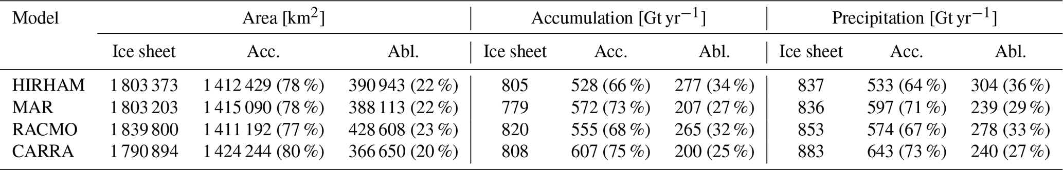
We define the accumulation zone using the mask presented in Vandecrux et al. (2019), which applies end-of-summer snow lines from Fausto et al. (2018) to identify the minimum firn area observed between 2000–2017. This region, covering 1 405 500 km², corresponds to the area where snow was persistent through the 2000–2017 period, with a boundary uncertainty of 1 %, estimated by shifting the firn line by ± 1 km (Fausto et al., 2018). Within the PROMICE ice mask, this firn area represents ∼ 80 % of the ice-sheet, with the remaining ∼ 20 % classified here as the ablation zone (Table 1).

Table 1 Ice-sheet area, accumulation and precipitation distribution across the PROMICE ice mask (Ice sheet), the accumulation (Acc.) and ablation (Abl.) zones, shown for the 1991–2022 overlap period.

2.3 SUMup In Situ Observational Data

The SUMup collaborative database is a compilation of in situ measurements of SMB as well as subsurface temperature and density for the Greenland and Antarctic ice sheets from published and unpublished sources (Vandecrux et al., 2024). The 2024 edition contains, in a harmonised format, over 2.4 million SMB values, of which > 2.1 million fall within the PROMICE ice mask, with ∼ 95 % located in the accumulation zone (Fig. 1). The data are derived primarily from airborne radar (Montgomery et al., 2020; Lewis et al., 2017; Koenig et al., 2016), ground based radar (Lewis et al., 2019; Miège et al., 2013), ice/firn-cores (Kawakami et al., 2023; Freitag et al., 2022a, b, c; Vinther et al., 2022; Osman et al., 2021; Lewis et al., 2019; Graeter et al., 2018; Miege et al., 2014; Miège et al., 2013; Box et al., 2013; Hanna et al., 2011; Burgess et al., 2010; Bales et al., 2009; Banta and McConnell, 2007; Hanna et al., 2006; Mosley-Thompson et al., 2001; Miller and Schwager, 2000b, c, d, a; Hammer and Dahl-Jensen, 1999; Clausen et al., 1988), snow pits (Kjær et al., 2021; Niwano et al., 2020; Schaller et al., 2016; Bolzan and Strobel, 2001a, b, 1999a, b, c, d, e, f, g, 1994), stake measurements (Chandler et al., 2021, 2015; Hermann et al., 2018; Machguth et al., 2016; Dibb and Fahnestock, 2004), SnowFox sensors (Fausto, 2021) and mass balance profiles (Machguth et al., 2016). An overview of their spatial coverage by decade and season is provided in Appendix Figs. A1 and A2, respectively.

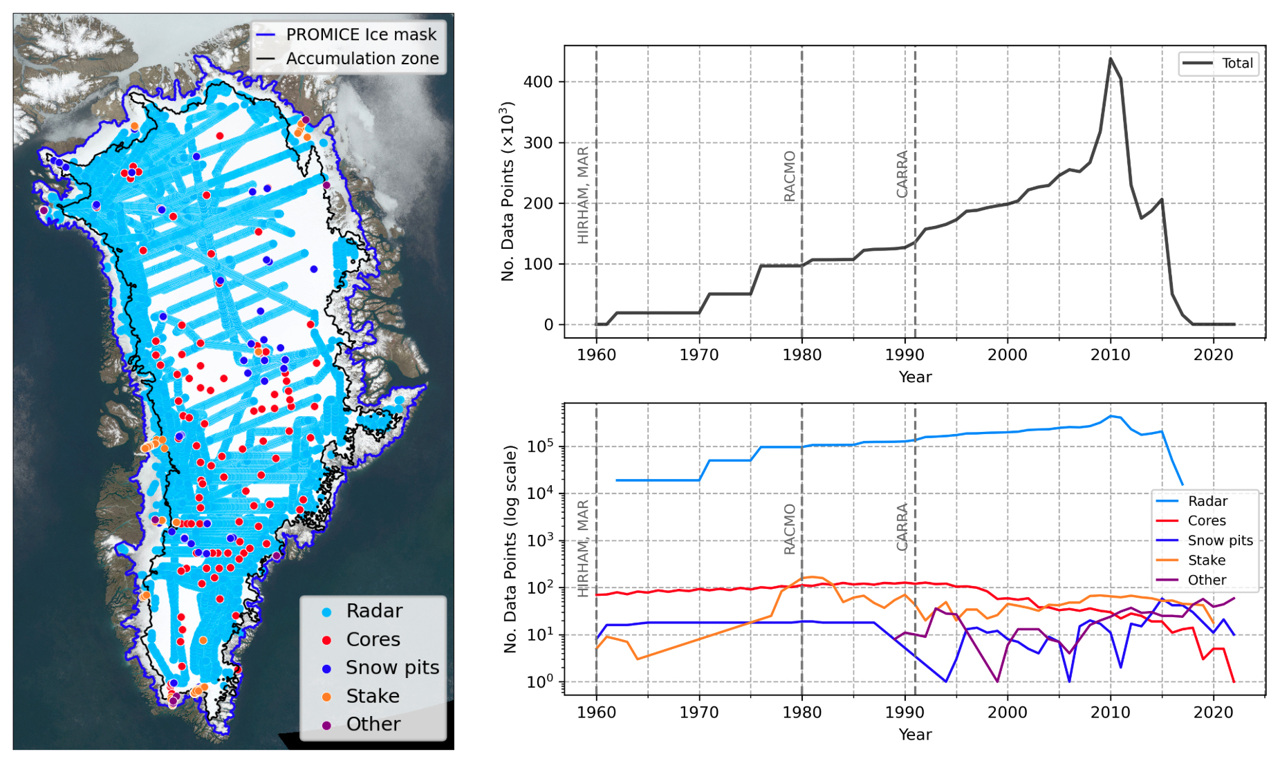
Figure 1 Left: geographical distribution of SUMup data points used in this study between 1960 and 2022, illustrated by measurement type. The method type “other” includes mass balance profiles and SnowFox sensors. Right upper: time dependence of total number of data points with markers for the start year of model data. Right lower: time dependence of data points by measurement type, with counts in log scale.

To focus on constraining accumulation and not runoff, for which SUMup data are not sufficient, we filter out negative SMB data in the ablation and percolation zones, thereby excluding measurements which may describe melt or runoff. This removes all data from automated weather stations, as well as a subset of those from stake measurements, SnowFox sensors, and mass balance profiles. Any measurements substantially impacted by melt are already excluded in the SUMup release. Consequently, we consider the remaining observations to represent a reliable dataset for comparison with model accumulation output.

Prior to bias-adjustment, SUMup data were inspected for potential issues, including inconsistencies arising from density conversions, processing or dating errors. For example, we found discrepancies between timestamps for Miège et al. (2013) radar data in the SUMup 2024 release and the related dataset Miege et al. (2014). After testing alternative interpretations, pre-summer start/end dates were set to 1 January/31 December, and post-summer dates to 1 January the following year/ 31 December, based on annualised rates in Miege et al. (2014), improving consistency with remaining data and model values.

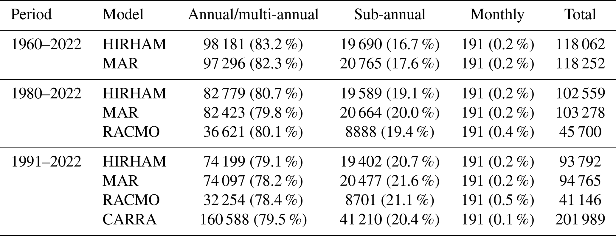
The temporal resolution of SUMup data varies between method types: ice cores, mass balance profiles and radar estimates (with the exception of surface layers) provide annual to multi-annual averages; snow pits span 5–12 months; stake measurements range from daily to 2 years; and SnowFox sensors record at weekly intervals. To align observations with monthly model outputs, sub-monthly data are resampled to monthly sums, and dates are rounded to nearest month boundaries. Measurements for which this rounding shifts the effective measurement period by > 15 % of its total duration are excluded to avoid introducing artificial biases from temporal misalignment. The resulting data comprises ∼ 80 % annual/multi-annual means (Table 2).

For measurements where only the start and end year are stated, dates are inferred from the original studies if possible. For example, some ice core studies using H₂O₂ dating use summer peaks (e.g. Kjær et al., 2021) to derive annual accumulation, and others mid-winter minima (e.g. Miège et al., 2013). Otherwise, default values corresponding to the first and last days of the reported year(s) are assigned, applying to 48 % of entries for 1960–2022, 43 % for 1980–2022, and 37 % for 1991–2022.

We assign a dating uncertainty (in months) to each SUMup record to account for errors in the temporal bounds. This uncertainty is derived from the original study if stated, otherwise, method-based default values are assigned based on those commonly stated literature. Radar and ice/firn-core measurements are assigned a default uncertainty of 12 months to account for potential missed annual layers; snow pits, for which precise start dates are unknown, are assigned 2 months; and stake measurements and SnowFox sensors with well-defined dates are assigned 0. The dating uncertainty is implemented as a Gaussian-weighted distribution, allowing model output to be bias-adjusted against each measurement within the specified uncertainty range.

Table 2 Number and percentage of observational data points fitted for each model and time period by temporal resolution.

The latitude and longitude coordinates of each measurement are matched with the nearest grid cell for each model. Radar data points from the same source and year range, which are thus not independent, are grouped and averaged within grid cells, reducing the computational time for the fit. This leads to a different numbers of data points fitted to each model (Table 2) and effectively smooths radar data to a greater degree for lower-resolution models.

3 Methods

3.1 EOF analysis

Our method relies on Empirical Orthogonal Function (EOF) analysis, performed on model accumulation output within the PROMICE ice mask, using the eofs.xarray module from the eofs Python library (Dawson, 2016).

The model output, $\mathbf{X}(x,y,t)$, is first centred by removing the temporal mean, M(x,y), and the climatology, $\mathbf{C}(x,y,m)$, where C is the mean deviation of each month, m, from the temporal mean. The EOFs, EOF(x,y), reveal the preferred patterns of spatial variability, while the principle components, PC(t), describe their monthly temporal evolution for each mode, i.

The reconstructed model accumulation, $\mathbf{Acc}(x,y,t)$, can thereby be expressed as:

$$\begin{array}{}\text{(8)}& \begin{array}{rl}\mathbf{Acc}(x,y,t)& =\mathbf{M}(x,y)+\mathbf{C}(x,y,m)\\ & +\sum _{i=\mathrm{1}}^N\mathit{P}{\mathit{C}}_i\left(t\right)\cdot {\mathbf{EOF}}_i(x,y).\end{array}\end{array}$$

We limit the adjustment to the first 10 EOF modes, capturing 86 %–91 % of the model variance while avoiding over-fitting noise captured in higher order modes. Using a truncation such as this, a residual term, $\mathbf{R}(x,y,t)$, is introduced to describe the remaining variability and noise. Further details of the EOF method are provided in Appendix A1.

3.2 The model

The SUMup dataset is used to find a set of coefficients to adjust each component of the accumulation reconstruction, derived by fitting the SUMup data points using the python package scipy.optimize.least_squares for least-squares optimisation (Virtanen et al., 2020). The bias-adjusted reconstructed accumulation, $\mathbf{Acc}(x,y,t)$, is then expressed as:

$$\begin{array}{}\text{(9)}& \begin{array}{rl}\mathbf{Acc}(x,y,t)& =a_{\mathrm{0}}+\mathbf{M}(x,y)+b_{\mathrm{0}}\mathbf{C}(x,y,m)\\ & +\sum _{i=\mathrm{1}}^{\mathrm{10}}\left(b_i\mathit{P}{\mathit{C}}_i\left(t\right)+a_i\right){\mathbf{EOF}}_i(x,y)\\ & +\mathbf{R}(x,y,t),\end{array}\end{array}$$

where a₀ adjusts the mean, M, a_i adjust the EOFs, EOF_i, b₀ adjusts the climatology, C, b_i adjusts the PCs, PC_i, and the truncation residual term, R is not adjusted. The initial guess (no adjustment) is set to 0 for the time-independent a parameters and 1 for the time-dependent b parameters. Using 10 EOFs results in 22 free parameters.

The dominant EOF patterns and associated PCs are often interpreted in terms of physical processes that drive climate variability, however, here they are solely used to create a smooth, reduced-dimensional basis for bias estimation.

We minimise the misfit between SUMup data and modelled accumulation using residuals scaled to an annual basis, giving greater weight to higher-resolution measurements. Due to the temporal uncertainty inherent in much of the SUMup dataset, of which ∼ 80 % consists of annual or multi-annual averages, the precise timing of individual accumulation events is often uncertain. To prevent over-fitting and mitigate the impact of dating errors, Tikhonov regularisation is applied to the b-parameters, constraining them towards the initial guess via a regularisation parameter λ. The optimum λ is found through 5-fold cross-validation, minimising the average mean squared error (MSE) of the residuals. To account for potential dependencies within SUMup, temporally or spatially linked measurements, such as data points from the same ice core, snow pit, stake network, or radar horizon, are assigned to the same fold during cross-validation; assignments are otherwise random. The optimal λ is determined independently for each model and evaluation period. For the 1991–2022 period, optimal λ values are 8.9 for HIRHAM, 15.8 for MAR, 8.9 for RACMO, and 12.6 for CARRA. For 1980–2022, λ values are 14.1 for HIRHAM, 11.2 for MAR, and 11.2 for RACMO, and for 1960–2022, optimal λ for HIRHAM and MAR are again 14.1 and 11.2.

To reduce the influence of outliers, several data transformations, including log and arcsinh, were tested and evaluated using the same cross-validation framework. However, as these provided no measurable improvement in fit quality, subsequent development was performed in linear space. As an alternative, the five loss functions available in the scipy.optimize.least_squares package were evaluated across a range of outlier threshold values (f_scale). The arctan loss function with f_scale=1 m yr⁻¹ yielded the greatest average reduction in MSE and was adopted across all models for consistency.

3.3 Bias Analysis

To assess the statistical significance of accumulation biases, we test the null hypothesis that the observed bias, defined as the difference between the original and adjusted fields, arises solely from inter-annual variability. Annual accumulation anomalies are modelled as a first-order autoregressive (AR(1)) process, with parameters estimated from the original model output. For each model and fitting period, we generate k AR(1) realisations of synthetic bias, whose cumulative sums form a Monte Carlo null distribution. Statistical significance is assessed using a two-sided p-value, defined as the fraction of simulations whose absolute cumulative bias exceeds that of the observed value. Implementation details are provided in Appendix A2.

For spatial patterns (Figs. 3, 4, A4), this test is applied independently at each grid cell, accounting for temporal autocorrelation but not spatial covariance. For domain-wide means (Tables 4, A1, A2, Fig. 4 (in-panel mean values)), the test is applied to a single spatially aggregated time series for each domain, such that p-values account for both temporal autocorrelation and implicitly for spatial covariance.

For Table 3, where metrics are derived from direct comparison between individual observations and corresponding model grid cell values over differing time scales (monthly to multi-annual), inter-annual variability cannot be defined in a consistent or meaningful way. Statistical significance of mean bias and RMSE changes is therefore assessed using 95 % confidence intervals obtained from 1000 non-parametric bootstrap resamples.

Bias-adjusted mean accumulation is reported with uncertainty intervals, estimated by spatial cross-validation. The adjustment model is trained by withholding observations from one of the seven basins and validated against the withheld data in turn. The uncertainty, σ, is expressed as the standard deviation of the seven reconstructions, R_i, relative to the full data mean, $\stackrel{\mathrm{‾}}{R}$:

$$\begin{array}{}\text{(10)}& \mathit{\sigma }=\sqrt{{\displaystyle \frac{\mathrm{1}}{\mathrm{7}}}\sum _{i=\mathrm{1}}^{\mathrm{7}}{\left({\stackrel{\mathrm{‾}}{R}}_i-\stackrel{\mathrm{‾}}{R}\right)}^{\mathrm{2}}}.\end{array}$$

This value, representing the sensitivity of the adjusted mean accumulation to variations in the training dataset, is hereafter referred to as the cross-validation uncertainty.

Model bias is quantified both as the net difference, B_net, between the original and bias-adjusted means, $\stackrel{\mathrm{‾}}{X}$ and $\stackrel{\mathrm{‾}}{X^{\prime }}$, and as a relative bias, B_rel, calculated at each grid point:

$$\begin{array}{}\text{(11)}& {\displaystyle }{B}_{\mathrm{net}}=\stackrel{\mathrm{‾}}{X}-\stackrel{\mathrm{‾}}{X^{\prime }},\text{(12)}& {\displaystyle }{B}_{\mathrm{rel}}={\displaystyle \frac{\stackrel{\mathrm{‾}}{X}-\stackrel{\mathrm{‾}}{X^{\prime }}}{\stackrel{\mathrm{‾}}{X}}}\times \mathrm{100}.\end{array}$$

The bias-adjustment is further evaluated through analyses of linear trends and accumulation sensitivity to temperature, assessed by grid-point-wise and domain-wide regressions. Sensitivity is defined as the percent change in accumulation per degree Celsius, derived from the Clausius-Clapeyron relationship (Clausius, 1850; Clapeyron, 2006) describing the saturation water vapour pressure, e_s as a function of temperature, T. Using a similar approach to Nicola et al. (2023) and Bochow et al. (2024), the Clausius-Clapeyron relationship can be expressed as:

$$\begin{array}{}\text{(13)}& {\displaystyle \frac{\mathrm{d}\ln e_{\mathrm{s}}}{\mathrm{d}T}}={\displaystyle \frac{L}{R_{\mathrm{v}}{T}^{\mathrm{2}}}}=k,\end{array}$$

where L is the latent heat of vaporisation, R_v is the specific gas constant for water vapour and k is the growth constant. Assuming precipitation, P, scales with saturation vapour pressure, its temperature response is commonly modelled via a log-linear relationship (Nicola et al., 2023; Bochow et al., 2024). We extend this approach to net accumulation, assuming that under cold, high-latitude conditions where sublimation and evaporation are minimal relative to precipitation, accumulation approximately scales with precipitation. Therefore, we fit ln(Acc) against Northern Hemisphere mean temperature anomalies from the Hadley Centre dataset (Morice et al., 2021, HadCRUT5 analysis), which combines near-surface (2 m) air temperature and sea surface temperature (SST) anomalies. The growth factor, k, is determined from the regression slope, and represents the fractional change in accumulation per degree Celsius. Following Bochow et al. (2024), the sensitivity, s, is defined as:

$$\begin{array}{}\text{(14)}& s=\mathrm{100}\times \left(e^k-\mathrm{1}\right),\end{array}$$

where s is the percent change in accumulation per degree of warming.

A sensitivity analysis comparing HadCRUT5 with Berkeley Earth (Rohde and Hausfather, 2020) and GISTEMP (Lenssen et al., 2024) confirms that the choice of dataset has negligible impact on the results over the post 1960 period investigated here.

4 Results

4.1 Bias-Adjustment Coefficients

Bias-adjustment coefficients indicate how each component of the model decomposition (Eq. 9) is scaled to fit SUMup data (Fig. 2). Adjusting the mean, a₀ is positive for HIRHAM, MAR and RACMO, reflecting a mean negative bias, and negative for CARRA, correcting a mean positive bias. The EOF coefficients (a₁–a₁₀) scale the amplitude of spatial variability patterns; HIRHAM shows the greatest spread, with a standard deviation of 0.004, while RACMO shows the smallest (0.002). Inter-model differences in EOF coefficients are associated with differing EOF patterns (Fig. A3), bias structures, and radar grouping.

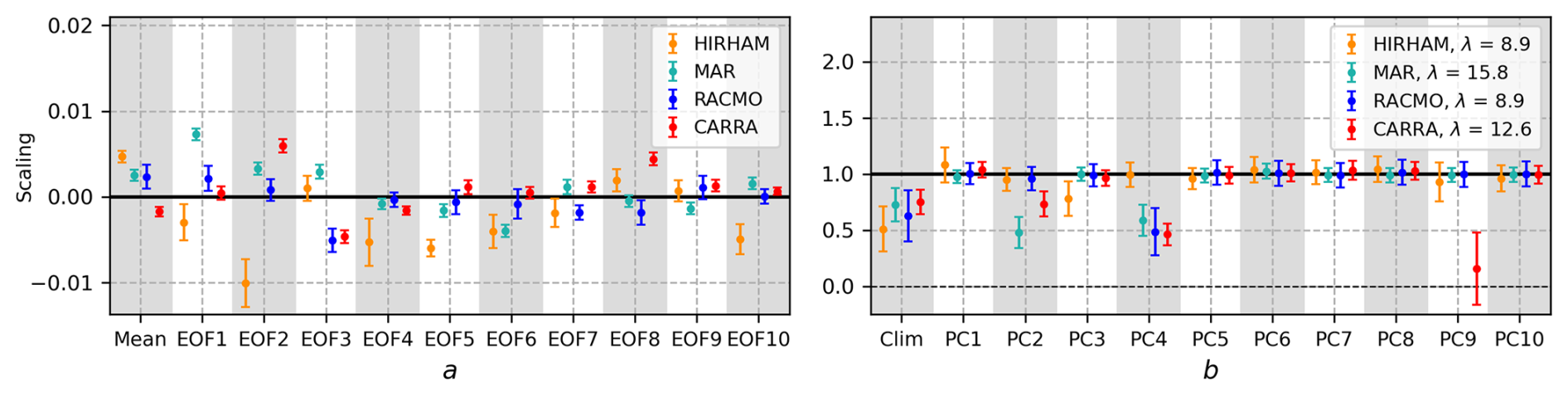
Figure 2 Bias-adjustment coefficients derived from fitting the 1991–2022 overlap period using the arctan loss function. Error bars represent the uncertainty in parameter estimates, reflecting the confidence in the fitted coefficients rather than spatial variability. The solid black line denotes the initial guess (no adjustment). Left: a parameters adjusting the time-independent mean and EOF patterns. Right: b parameters adjusting the time-dependent climatology and PC modes, with λ values derived independently for each model via cross-validation.

The temporally dependent b coefficients are influenced by the regularisation parameter, λ, which penalises deviations from the initial guess to account for the uncertainty in observational dating; higher λ values impose stronger constraints. Adjusting the climatology, b₀ is scaled down for all models to between 0.51 (HIRHAM) and 0.75 (CARRA), reflecting smoothing of sub-annual variability due to the dominance of annual/multi-annual measurements (∼ 80 %; Table 2). Most PC adjustment coefficients (b₁–b₁₀) remain close to the initial guess, with a few notable exceptions (MAR PC2, PC4 for MAR, RACMO and CARRA, and CARRA PC9). Despite the strongest regularisation, MAR (λ=15.8) and CARRA (λ=12.6) PC coefficients show the greatest spread, with standard deviations of 0.18 and 0.29, respectively, driven by strong scaling of a few coefficients.

4.2 Bias-Adjustment Assessment Metrics

Prior to bias-adjustment, CARRA exhibits the largest statistically significant mean point-wise bias of +10.1 % compared to observations (Table 3), followed by HIRHAM with consistent significant negative mean biases of −7.5 % to −7.4 %. MAR exhibits small initial biases, which are statistically significant in the 1960–2022 (−0.5 %) and 1991–2022 (+0.7 %) fitting periods. RACMO is the only model to show non-significant negligible mean bias (∼ 0 %) in both fitting periods.

Table 3 Model mean bias, root mean square error (RMSE), and correlation (R) before and after bias-adjustment, based on a point-wise comparison with SUMup data (with radar values averaged within grid cells). Bias is expressed as the mean percentage deviation relative to SUMup, $\mathrm{100}\times \langle \text{model}-\text{SUMup}\rangle /\langle \text{SUMup}\rangle$. Bold values indicate statistically significant mean bias or RMSE improvement.

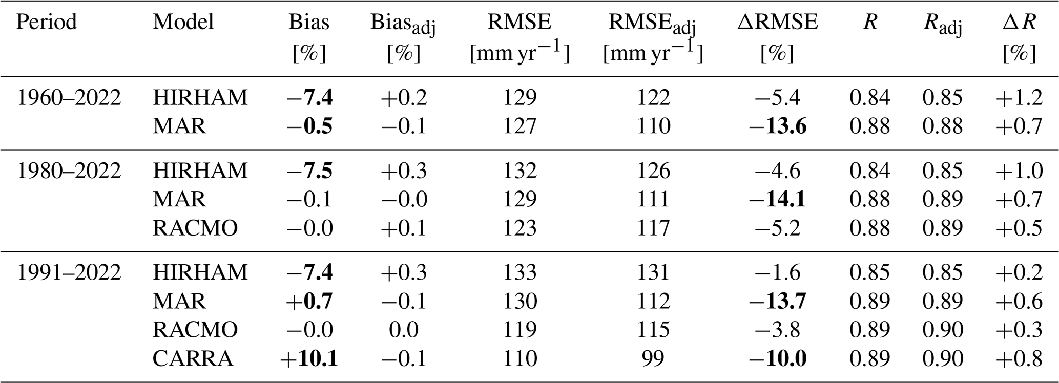
After adjustment, mean bias is reduced to near-zero in all models (± 0.3 %). RMSE decreases by 1.6 %–14.1 %, representing significant reductions for MAR and CARRA, while correlation improves modestly by 0.3 %–1.2 %.

4.3 Mean Accumulation and Spatial Bias Patterns

Before bias-adjustment, all models share similar mean accumulation patterns. The large-scale remains largely unchanged after adjustment, however, marked differences in spatial bias patterns reveal considerable differences between models (Fig. 3).

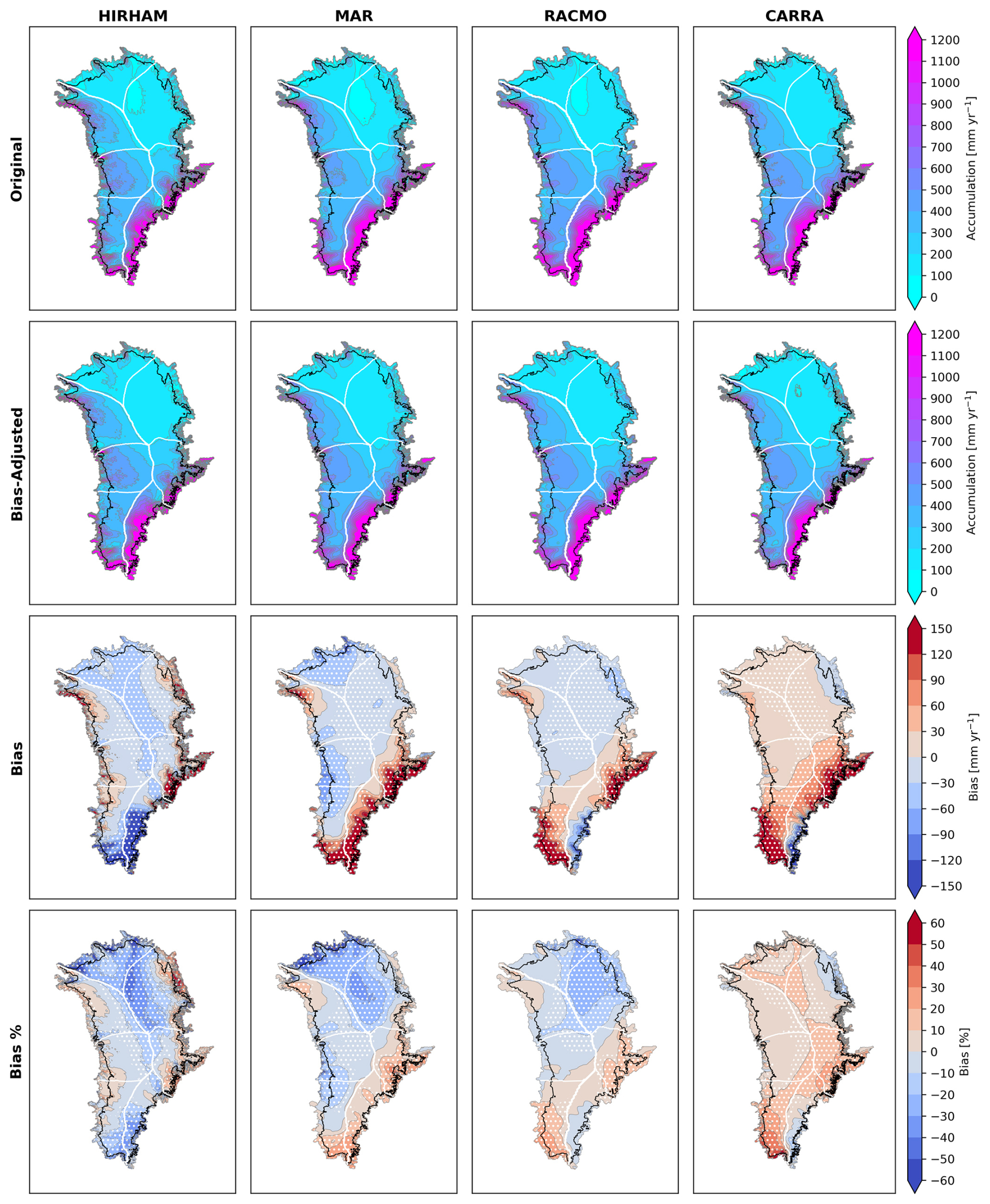
Figure 3 Model mean accumulation and bias patterns over 1991–2022. First row: original mean model accumulation. Second row: bias-corrected mean accumulation. Third row: mean net bias (mm yr⁻¹) (Eq. 11). Fourth row: mean relative bias (Eq. 12). Hatched regions indicate statistically significant biases (p<0.05). The black line indicates the accumulation zone boundary, and white lines show PROMICE drainage basins boundaries. Maps for full model periods are provided in Appendix Fig. A4.

HIRHAM, MAR and RACMO are consistently biased low in mean relative bias over all periods (Table 4). In HIRHAM, significant negative bias dominates most of the ice-sheet, reaching −50 % in the north and north-east (Fig. 3), while high-accumulation regions in the south-west and south-east contribute disproportionately to net bias, with significant underestimation locally exceeding −150 mm yr⁻¹. MAR also underestimates across much of the ice-sheet, with significant biases reaching −40 % in the north and north-east, but differs from HIRHAM through a pronounced fringe of significant positive bias in the south and central-east, exceeding +150 mm yr⁻¹. RACMO shows the smallest mean ice-sheet-wide relative bias of −4 % in both fitting periods. Negative relative bias is most prominent in the north-east, reaching up to −30 %, while the south-west and central-east are biased high, exceeding +150 mm yr⁻¹ locally. Unlike MAR, RACMO exhibits a narrow region of non-significant negative bias in the south-east, reaching up to −120 mm yr⁻¹.

Mean relative bias decreases in later fitting periods for HIRHAM and MAR, while RACMO remains constant (Table 4).

CARRA shows the only positive mean relative bias of +9 % over the ice sheet. The largest net biases are similarly associated with high-accumulation regions, locally exceeding +150 mm yr⁻¹ in the south-west and central-east. Like RACMO, CARRA exhibits a narrow band of negative bias along the south-east margin, with values exceeding −150 mm yr⁻¹.

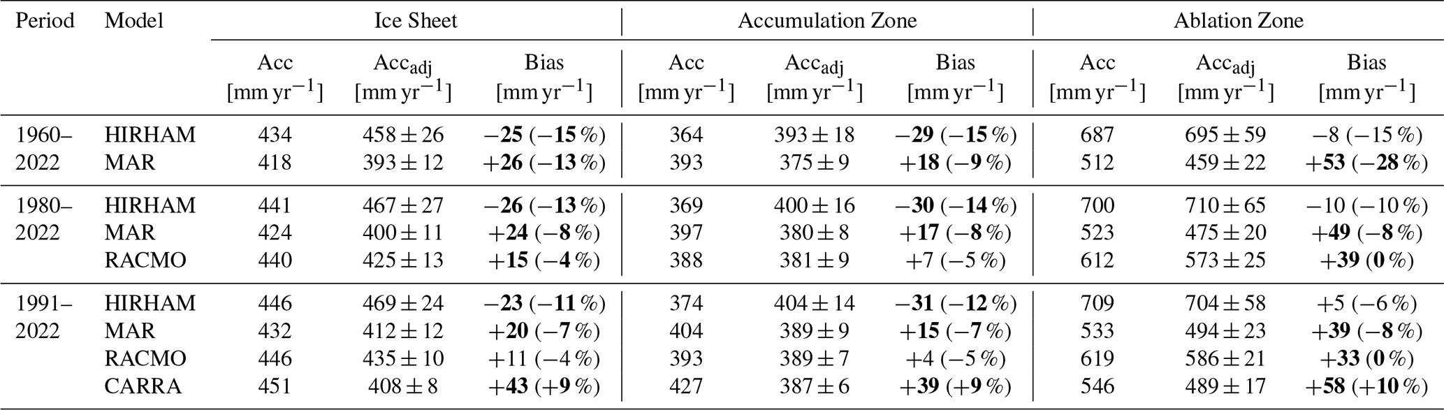
Within the observation-rich accumulation zone, bias-adjustment improves inter-model agreement in mean accumulation estimates (Table 4). For 1991–2022, inter-model standard deviation is reduced by 68 %, with MAR, RACMO, and CARRA converging closely, scaled down to 389 ± 9, 389 ± 7 and 387 ± 6 mm yr⁻¹, respectively. HIRHAM, however, is scaled up from 374 mm yr⁻¹ to 404 ± 14 mm yr⁻¹, falling outside the uncertainty bounds of other models.

In the sparsely sampled ablation zone, inter-model standard deviation increases from 68 to 86 mm yr⁻¹ after adjustment (1991–2022), with larger cross-validation uncertainties reflecting greater spread between individual reconstructions. This disparity in the ablation zone drives an increase in ice-sheet-wide inter-model standard deviation from 7 to 24 mm yr⁻¹.

Table 4 Mean annual accumulation before (Acc) and after adjustment (Acc_adj) over the ice sheet, accumulation zone, and ablation zone, with corresponding mean bias. Bias-adjusted values are shown with cross-validation uncertainties (Eq. 10). Bias is reported as the mean net difference (Eq. 11) and mean relative bias (Eq. 12). Statistically significant biases (p<0.05) are highlighted in bold. Equivalent spatially aggregated sums (Gt yr⁻¹) are provided in Appendix Table A1, with the temporal evolution of net and cumulative bias shown in Fig. A5.

With the exception of RACMO over the 1991–2022 period, all ice-sheet–wide mean biases are statistically significant (Table 4). Basin-wise means (Table A2) reveal that bias in the north, central-east and south-west basins is significant in all models, with the south-west representing the greatest net and relative biases for RACMO (+20 to +26 Gt yr⁻¹; +14 % to +19 %) and CARRA (+34 Gt yr⁻¹; +25 %). Bias in the south-east basin is also significant for HIRHAM (−39 to −54 Gt yr⁻¹; −17 % to −25 %) and MAR (+30 to +33 Gt yr⁻¹; +14 % to +16 %), constituting their largest net biases, while non-significant for RACMO and CARRA (within ± 2 %). The north-east basin is significant for MAR and RACMO (all periods) and HIRHAM (1960–2022, 1980–2022), while MAR and CARRA also show significant biases in the central-west basin. The north-west basin is not statistically significant for any model and consistently exibits the smallest net and relative biases.

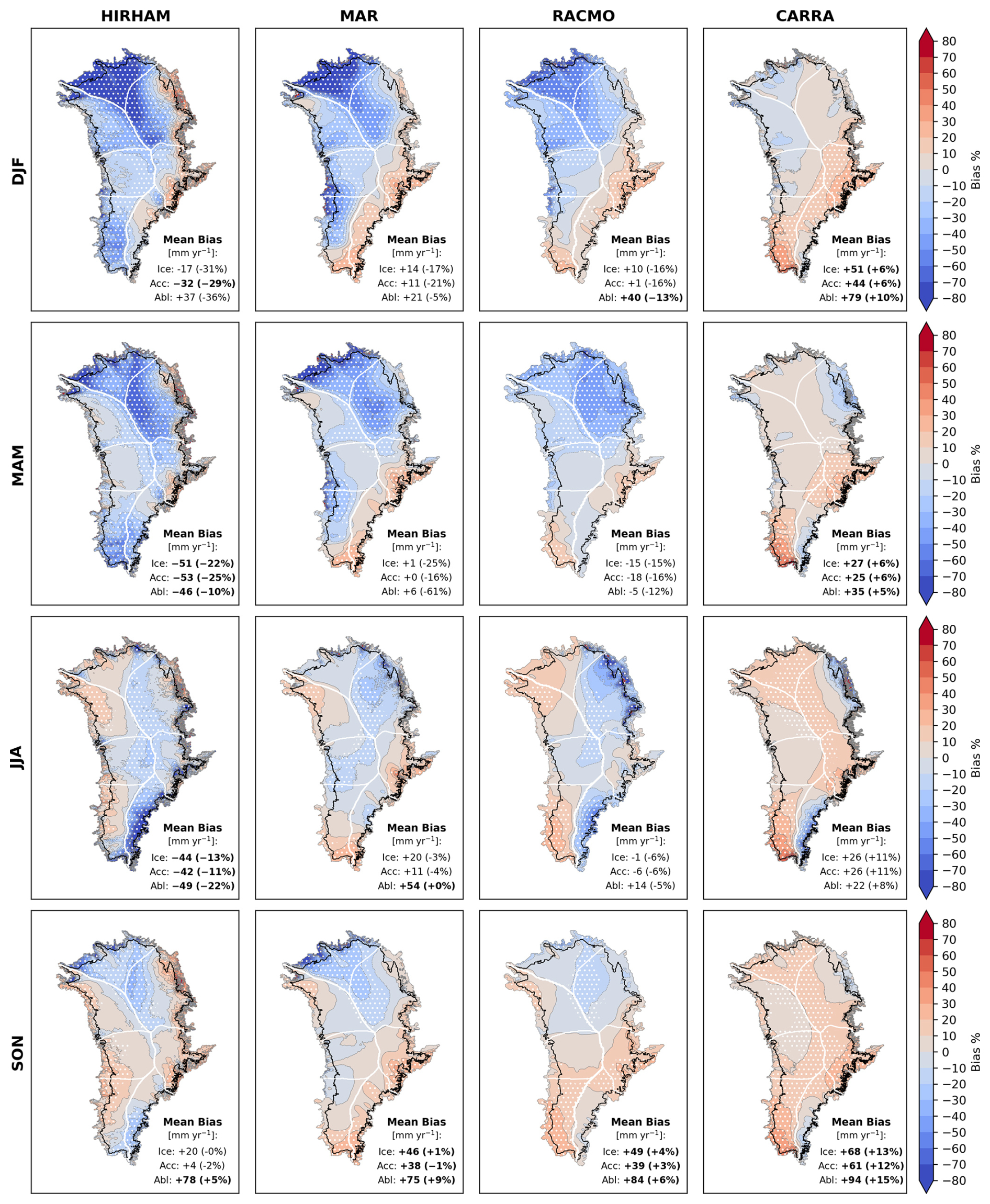
Figure 4 Model mean seasonal relative bias over the 1991–2022 common period, calculated by Eq. (12) for each season. Hatched regions indicate statistically significant biases (p<0.05). In-panel labels show seasonal mean bias values over the ice-sheet (Ice), accumulation zone (Acc) and ablation zone (Abl), with statistically significant biases indicated in bold.

4.4 Seasonal Bias Patterns

Seasonal pattern biases show strong seasonal contrasts (Fig. 4). All models show a seasonal shift in ice-sheet-wide relative mean biases, from more negative (or less positive) in colder months towards least negative (or most positive) in autumn.

For HIRHAM, MAR and RACMO, the greatest negative relative biases occur in winter and spring, accompanied by the most spatially extensive regions of statistically significant bias. Significant negative biases are concentrated in the north and north-east across all three models, extending to the south for HIRHAM and MAR. In summer, these models exhibit an expanded area of positive relative bias (up to ∼ 20 %) in the north-west, which retreats towards central regions in autumn.

In domain-wide means, HIRHAM biases are significant across all domains in spring and summer, coinciding with the seasons of greatest negative net ice-sheet–wide bias, while MAR and RACMO show their largest and statistically significant net mean biases across all domains only in autumn. CARRA maintains positive mean bias throughout the year, significant in all seasons except summer. Mean relative bias is lowest in winter and spring and highest in autumn, coinciding with the greatest mean net bias and most spatially extensive significant biases.

4.5 Temporal Trends

Spatial patterns of temporal trends reveal a pronounced east-west contrast in all models (Fig. 5). Positive trends dominate in the east and largely negative trends in the west. This behaviour is mostly preserved after adjustment, with a few exceptions; HIRHAM shows slightly expanded positive regions in the north-west basin, while isolated areas of positive trends present prior to adjustment in MAR, RACMO and CARRA become negative in this basin. Consequently, spatial patterns and basin-wise means (Table A3) in MAR, RACMO and CARRA show closer agreement after adjustment, while HIRHAM diverges.

In all models, the strongest trends occur in the south-east, with basin mean values of up to +66.0 mm yr⁻¹ decade⁻¹ (Table A3), contrasted with negative means in the south-west of up to −15.5 mm yr⁻¹ decade⁻¹.

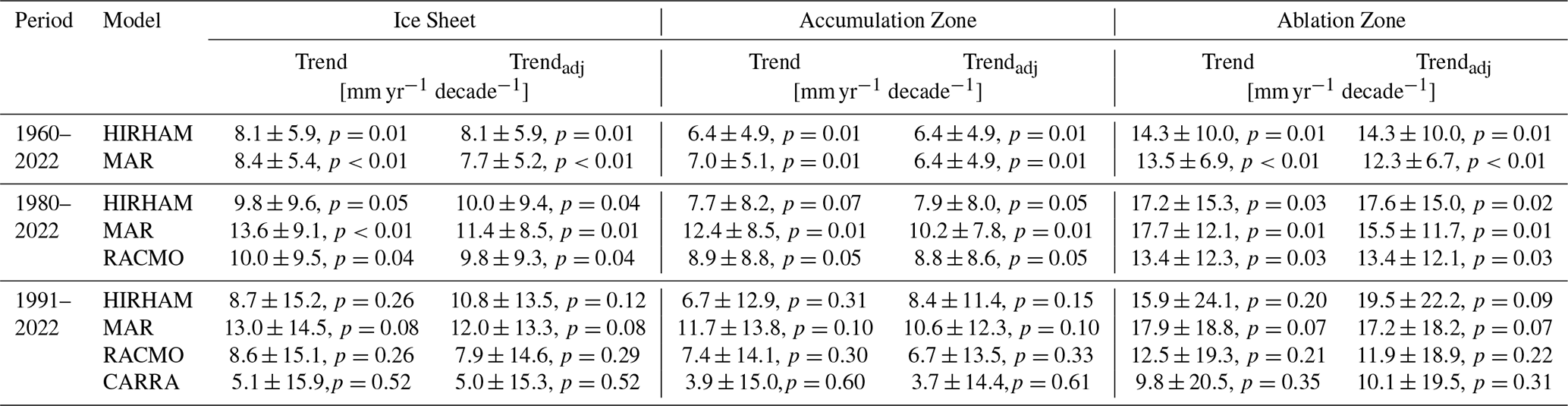
Domain-wide mean trends are positive across all models and fitting periods (Table 5), and bias-adjustment generally leads to a small reduction in trend magnitude (typically ≤ 2 mm yr⁻¹ decade⁻¹). Notable exceptions include HIRHAM (all domains) and CARRA (ablation zone), for which bias-adjustment maintains or slightly increases trend magnitudes. MAR shows the strongest mean trends overall, coupled with the lowest p-values, while CARRA shows the weakest trends and highest p-values. Confidence intervals widen and p-values increase as earlier data are excluded from the fitting period, reflecting the reduced temporal coverage and greater influence of inter-annual variability in shorter records.

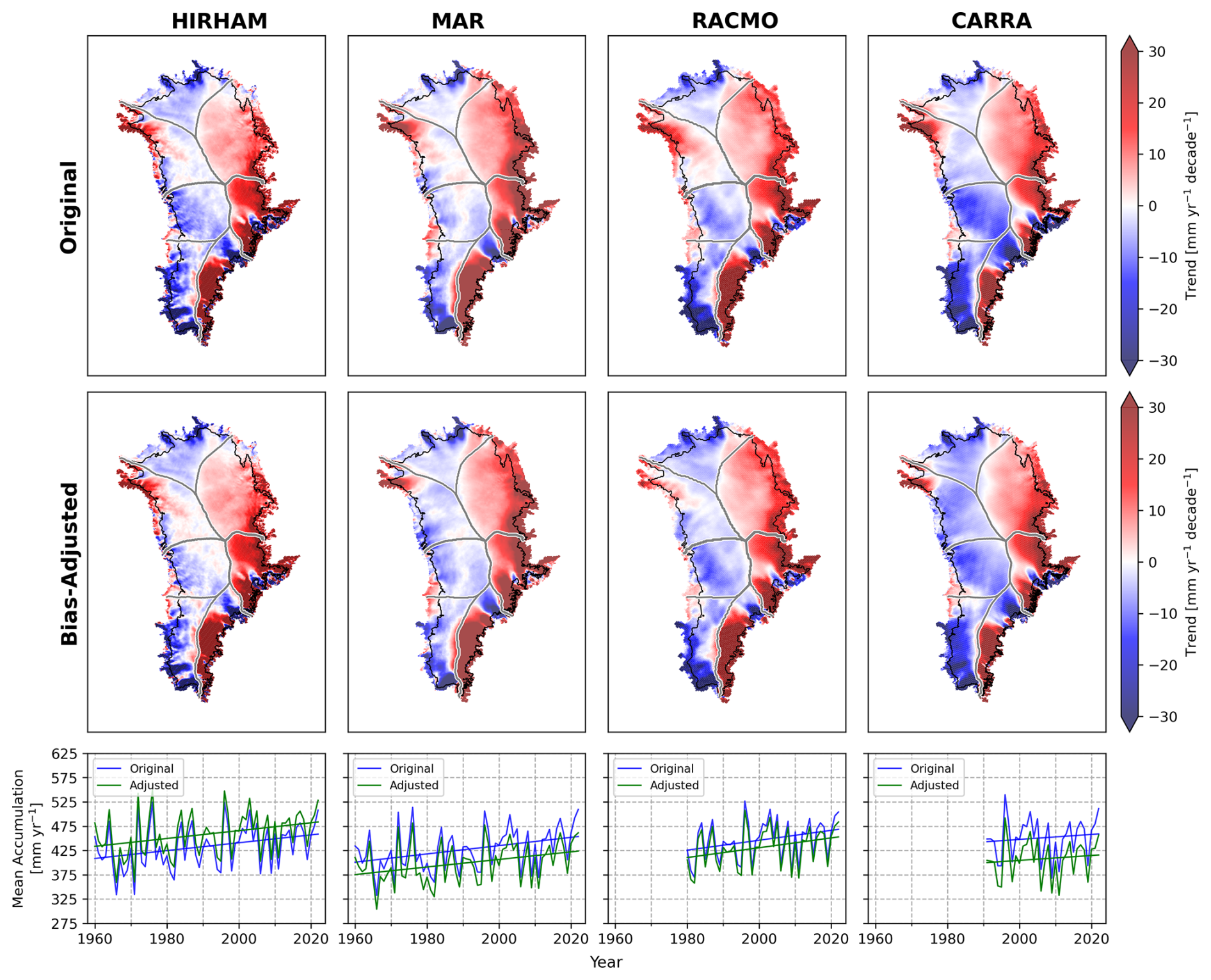
Figure 5 Temporal regressions before and after bias-adjustment. Upper: grid-point-wise regression over 1991–2022. Lower: mean annual accumulation over the ice sheet with linear fits for HIRHAM and MAR (1960–2022), RACMO (1980–2022) and CARRA (1991–2022).

Table 5 Spatial mean linear trends in accumulation over the ice sheet, accumulation zone, and ablation zone before and after bias-adjustment. Trends are reported with confidence intervals and p-values. Basin-wise mean trends are provided in appendix Table A3.

4.6 Temperature Sensitivity Analysis

Spatial temperature sensitivity patterns (Fig. 6) share a similar structure to the temporal regression patterns. MAR shows the strongest positive sensitivities, concentrated in the north- and south-east, exceeding +25 % K⁻¹ locally, coupled with the strongest domain-wide mean responses (Table 6). CARRA shows the most widespread negative sensitivities, reflected by the weakest domain-wide mean responses. Bias-adjustment reduces positive sensitivities in the north-west for MAR, RACMO and CARRA, resulting in near zero basin-wise mean responses for 1991–2022 (Table A4), while HIRHAM's positive mean trends in the north-west basin remain relatively consistent.

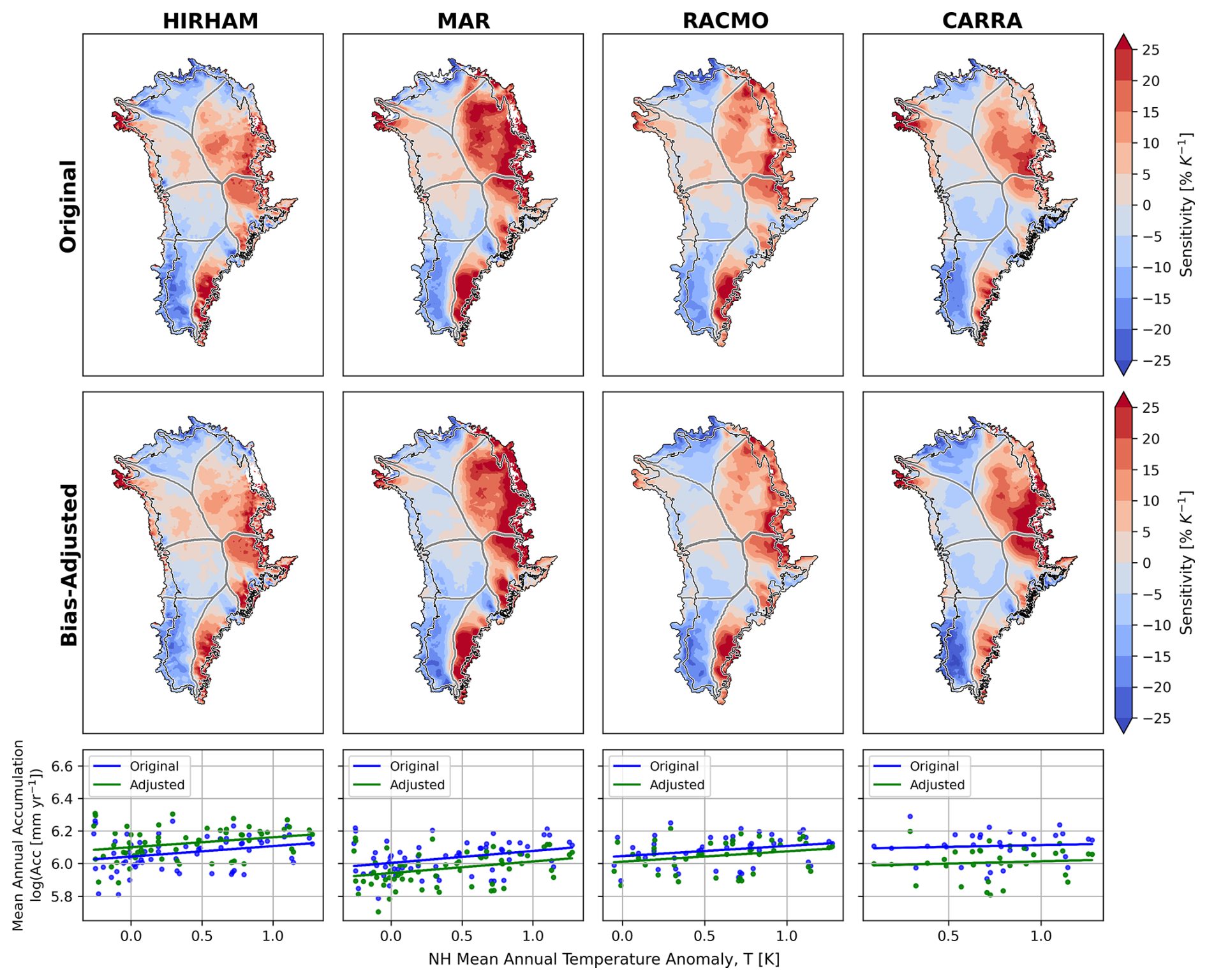
Figure 6 Temperature sensitivity analysis following Eq. (13). Upper panels show spatial sensitivity patterns over 1991–2022, derived from grid-point-wise linear regressions of log-transformed annual accumulation against HadCRUT5 NHT anomalies. Empty grid points from negative accumulation values are excluded from mean sensitivity calculations. Lower panels show ice-sheet-wide log-scale mean annual accumulation against NHT anomalies with linear fits for HIRHAM and MAR (1960–2022), RACMO (1980–2022) and CARRA (1991–2022).

Table 6 Mean spatial (grid-point wise) and temporal (ice-sheet-wide) accumulation sensitivities derived from linear regressions of log-transformed model accumulation against HadCRUT5 NHT anomalies before (S) and after bias-adjustment (S_adj). Basin-wise spatial mean sensitivities are provided in Appendix Table A4.

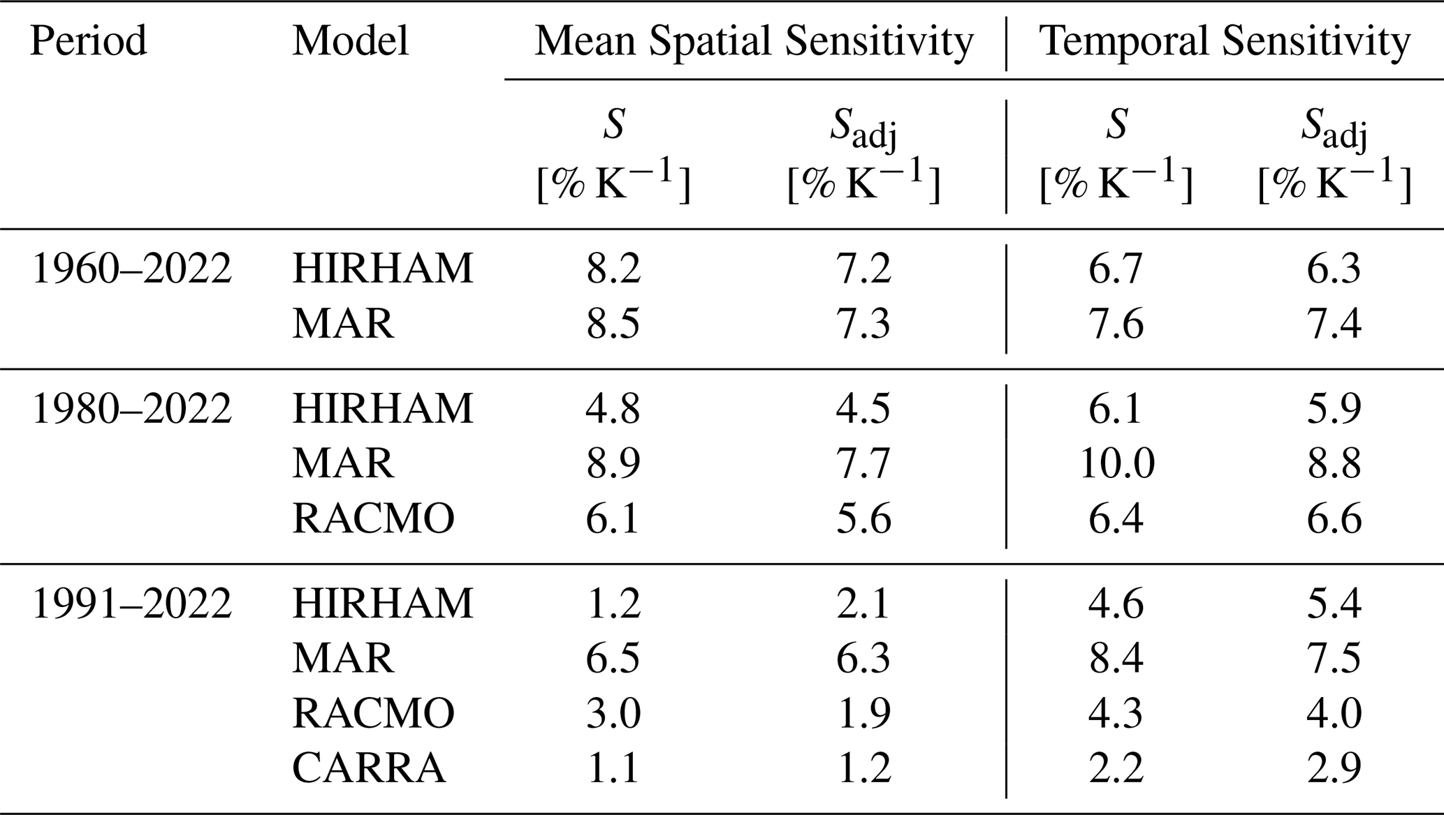
Mean spatial sensitivities, calculated as the grid-point average of localised responses, differ systematically from the temporal regression-derived sensitivities, which reflect the ice-sheet's integrated response to inter-annual temperature variability (Table 6). With the exception of the 1960–2022 period, temporal sensitivities exceed spatial averages. For 1991–2022, CARRA shows the lowest mean sensitivities, with an ice-sheet-wide temporal mean approximately four times lower than MAR, and six times lower in the spatial mean.

Bias-adjustment generally reduces both spatial and temporal sensitivity means (Table 6), with the exception of HIRHAM and CARRA for the 1991–2022 period and RACMO for 1980–2022, for which sensitivities increase slightly following adjustment.

5 Discussion

5.1 Mean Bias and Spatial Patterns

Our results indicate statistically significant ice-sheet-wide mean biases of 4 %–15 % are present in all models (Table 4), corresponding to 20–77 Gt yr⁻¹ (Table A1). Although modest on an annual basis, such biases accumulate substantially over time (Fig. A5). Over a century long simulation, a persistent 10 % bias would amount to ∼ 8000 Gt, sufficient to alter sea-level rise projections by approximately 25 mm by 2100 (The IMBIE Team, 2020). Using the empirical SMB-temperature relationship from AR5 (Intergovernmental Panel On Climate Change, 2014, Chap. 13 Supplement), an ∼ 80 Gt yr⁻¹ SMB deviation corresponds to an equivalent warming bias of ∼ 1 °C. This represents a substantial error relative to critical thresholds for GrIS stability, such as the ∼ 1.6 °C threshold identified by Robinson et al. (2012), beyond which irreversible long-term mass loss is expected. If uncorrected, such biases could obscure or misrepresent the proximity to climate tipping points.

Despite low mean biases in MAR and RACMO (Tables 3, 4, A1), consistent with Fettweis et al. (2020), who show MAR3.9.6 and RACMO2.3 outperform 13 other models against against GrIS-wide observations, our spatial analysis shows that these low means mask compensating significant opposing regional biases (Fig. 3, Table A2), including areas which may exert disproportionate influence on sea-level rise. Mouginot et al. (2019) identify the north-west, south-east, and central-west as the primary contributors to GrIS mass loss since 1972, with 34 % of total mass loss attributed to SMB changes. We find MAR exhibits significant biases in two of these regions: +9 % (+9–12 Gt yr⁻¹) in the south-east and −8 %–9 % (−6–7 Gt yr⁻¹) in the central-west.

HIRHAM and CARRA exhibit more spatially consistent low and high biases, respectively, with larger significant point-wise (Table 3) and ice-sheet-wide biases (Table 4). HIRHAM, however, is the only model with non-significant ablation-zone bias, aligning with Fettweis et al. (2020) who find HIRHAM outperforms other models against observations in the ablation zone.

While we find CARRA, biased high by a mean of +9 %–10 % (Tables 3, 4), performs worse than MAR and RACMO, recent studies have found CARRA shows better agreement with observations than other models. Evaluating CARRA and RACMO2.3p2 against daily snow depth data from nine Greenland coastal stations, van der Schot et al. (2024) report correlations are generally higher for CARRA than RACMO, with no clear over- or underestimation from either model. Similarly, Box et al. (2023) evaluate CARRA, ERA5, NHM-SMAP, RACMO2.3p2 and MARv3.11.5 against precipitation data from seven automated weather stations in two regions, including four on the ice-sheet, finding CARRA has the lowest mean bias.

The CARRA Data User Guide (Copernicus Climate Change Service, 2021) highlights that the model shows improved agreement with observations of high-precipitation events relative to ERA5, whose coarser resolution limits its ability to predict extremes. However, they note CARRA tends to overestimate precipitation compared to in situ observations over northern Scandinavia. Higher-resolution models better resolve complex topography and associated mesoscale circulation, enhancing orographic precipitation (Lucas-Picher et al., 2012). While this can improve representation of intense precipitation events, it may also result in higher mean precipitation relative to coarser-resolution products. Similar resolution-dependent increases in precipitation have been documented for RCMs over Greenland, where downscaling from ∼ 5 to ∼ 1 km leads to enhanced precipitation, particularly through increased rainfall (Huai et al., 2022). Consequently, CARRA’s tendency towards overestimation may be linked to its higher spatial resolution and sensitivity to orographically driven precipitation extremes.

Common to all models is a strong bias in the south; a region characterised by high snowfall and mountainous topography. Previous studies have identified the south-east, in particular, as a significant source of uncertainty, due to high spatial variability, complex orographic effects and limited observational coverage (Fettweis et al., 2020; Ryan et al., 2020; Koenig et al., 2016; Miège et al., 2013; Burgess et al., 2010). Notably, HIRHAM significantly underestimates in the south-east basin by a mean of up to −25 % (Table A2). Lucas-Picher et al. (2012) compare HIRHAM accumulation with ice cores from Andersen et al. (2006); Banta and McConnell (2007) and Bales et al. (2009), finding southern biases generally < 10 %. Our analysis, using a substantially larger observational dataset including radar-derived accumulation and covering previously unsampled areas, indicates that earlier evaluations may have underestimated biases near the complex south-eastern margin.

The northern interior of the ice-sheet contributes disproportionately to relative bias in HIRHAM, MAR and RACMO, with significant local biases of up to 30 %–50 % (Fig. 3). This may reveal a shared tendency to underestimate accumulation at cold, dry, high elevation sites, where atmospheric moisture is limited and snowfall events are infrequent, but significant for accumulation. Langen et al. (2017) also report that at high-elevation sites, HIRHAM5 underestimates net accumulation by 8 %–16 %.

While the north interior benefits from relatively consistent observational coverage through time, the south-east has sparse coverage prior to 2000 (Fig. A1), and the south-west remains poorly sampled throughout. As a result, adjustments in the south are less well constrained, particularly in earlier periods, contributing to greater uncertainty in both regions. Observations also become increasingly uncertain further back in time: deeper ice-core layers are more prone to miscounting (Steig et al., 2005), and radar horizons more likely to be misidentified (Bingham et al., 2025), which may lead the bias-correction to apply larger, possibly unnecessary, adjustments. Furthermore, the number of observations assimilated into ERA5, providing boundary conditions for all models, declines drastically in earlier decades (Hersbach et al., 2019), degrading model performance in the past. These factors may contribute to the reduction in mean relative bias in later fitting periods (Table 4).

5.2 Seasonal Bias and Spatial Patterns

The observed seasonal shift in ice-sheet-wide mean biases may reflect seasonally varying climatic processes that influence model performance differently over the year. While CARRA exhibits statistically significant mean biases in all seasons except summer, HIRHAM shows significant mean biases primarily in spring and summer, and MAR and RACMO primarily in autumn (Fig. A2). Seasonal biases, however, must be interpreted in light of the temporal limitations of the observations, of which 0.1 %–0.5 % are monthly measurements, while ∼ 80 % are annual/multi-annual means (Table 2), with dating often estimated from measurement peaks or melt horizons. These dating assumptions, which vary between sources, combined with the filtering of negative SMB data, particularly affect the robustness of spring and summer bias estimates. These factors leave a small fraction with which to reliably constrain bias patterns on a seasonal scale, making them inherently less robust than the annual means.

5.3 Temporal Trends and Temperature Sensitivity

The tendency for the bias-correction to temper mean accumulation trends for MAR, RACMO and CARRA may indicate that these models are overly sensitive to warming air temperatures, while HIRHAM, whose trends are slightly amplified by the adjustment, may be under-sensitive. However, this apparent sensitivity may be linked to model bias structures and stronger corrections applied to earlier, less well-constrained periods. All models show strong trends in the high accumulation south, coinciding with where net biases are largest (Fig. 3) and observations are sparse in earlier periods (Fig. A1). For MAR, RACMO and CARRA, with high positive biases dominating in the south, bias-adjustment reduces accumulation means on average, more strongly in earlier periods fitting periods (Table 4). Conversely, for HIRHAM, initially biased low in the south, mean accumulation is scaled up by the adjustment, more so in earlier periods.

HIRHAM and MAR's longer historical coverage (1960–2022) provides more statistically robust estimates, supported by lower uncertainties and p-values of ≤ 0.01. These longer-term trends are more resilient to inter-annual variability, which can dominate shorter records and obscure underlying trends. As such, the longer records provided by HIRHAM and MAR spanning 1960–2022, likely provide the most statistically reliable estimate of long-term accumulation trends, due to their extended temporal coverage. Although spatial trend patterns are illustrated for the shorter 1991–2022 period, the strong consistency in the sign and structure across models suggests that the broad-scale spatial contrasts, particularly the east–west contrast and strong southern gradients, are robust features (Fig. 5).

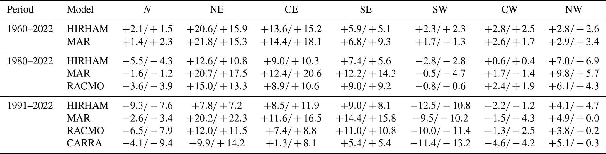
Similarly, spatial temperature sensitivity patterns (Fig. 6) are largely consistent between models. The patterns identified here share several consistent features with regional sensitivities reported in Buchardt et al. (2012). In the south-east, where they report sensitivities of +8.2 ± 0.8 % K⁻¹, we find basin-mean values ranging from +5.4 to +15.8 % K⁻¹ (Table A4). In the south-west, their reported sensitivity of −4.0 ± 0.1 % K⁻¹, corresponds to predominantly negative basin-mean sensitivities in our analysis of −13.2 % K⁻¹ to +2.3 % K⁻¹. Similarly, in the central-east, where Buchardt et al. (2012) find high sensitivity (+9.2± 1.0 % K⁻¹), adjusted values range from +8.1 % K⁻¹ to +20.6 % K⁻¹.

In the central-west, however, where Buchardt et al. (2012) report their highest sensitivity (+9.4± 0.1 % K⁻¹), we find moderate values, which are further reduced or become negative following adjustment, ranging from −4.2 % K⁻¹ to +2.5 % K⁻¹. Conversely, we find our highest sensitivities in the north-east basin ranging from +7.2 % K⁻¹ to +22.3 % K⁻¹ after adjustment, while Buchardt et al. (2012) report their lowest sensitivities of +1.5± 2.8 % K⁻¹. These discrepancies may reflect a temporal shift in accumulation sensitivity in these regions, as Buchardt et al. (2012) derive their estimates from ice cores primarily drilled in the 1970s and 1980s. Meanwhile, the strong east–west contrast in the south and high sensitivities in the central-east basin are consistent features, suggesting these patterns have persisted over time.

5.4 Limitations

The results presented in this study are subject to a number of methodological and observational limitations, which influence the magnitude, spatial structure and inter-model agreement in the final bias-adjusted accumulation, trend and sensitivity estimates.

Firstly, the EOFs are statistical constructs, which represent differing patterns of variability between models (Fig. A3) and fitting periods. Differences in EOF patterns, and in how each mode is scaled by the adjustment, may contribute to inter-model differences in the bias-adjusted results. By construction, the EOF approach introduces a degree of spatial smoothing, meaning that highly localised differences in accumulation captured in the observations may not be fully represented in the adjusted fields. In this study, we retain 10 EOFs, while higher-order modes account for an additional 8 %–14 % of the variance. These modes may represent physically meaningful variability rather than noise, and distinguishing signal from noise at these scales is non-trivial. A sensitivity test retaining up to 15 EOFs shows slight changes in spatial bias patterns and mean accumulation values. Increasing the truncation from 10 to 15 EOFs reduces the 1991–2022 inter-model standard deviation in ice-sheet-wide accumulation means from 23 to 20 mm yr⁻¹, though both remain higher than the pre-adjustment value of 5 mm yr⁻¹. While small relative to the overall inter-model spread, this change indicates the adjustment is sensitive to such methodological choices.

In addition, the robust loss function, which down-weights extreme deviations while preserving overall model–data agreement, may contribute to occasional apparent over-corrections in the adjustment, further contributing to increased inter-model spread. For example, HIRHAM shifts from a point-wise mean bias of −7.4 % to a slightly positive bias of +0.3 % (Table 3), and is scaled upwards beyond uncertainty ranges of other models in accumulation zone means (Table 4), which otherwise converge within ± 2 mm yr⁻¹. Consequently, cross-validation uncertainties may be underestimated; a complementary measure could use the spread across the four bias-adjusted means, capturing inter-model differences in addition to training-sample uncertainty.

Despite uncertainties associated with the method, comparison of bias patterns (Fig. 3, row 3) with point-wise spatial biases (Fig. A6) lends confidence that the method successfully captures the dominant bias structures indicated by the observations.

Ultimately, our results are intrinsically dependent on the quality, representativeness and temporal coverage of the observational data used for bias-adjustment. Though the ∼ 2 million data points in SUMup provide substantial statistical power compared to smaller-scale studies, observational uncertainties limit the accuracy of the final products. Through detailed inspection of the SUMup database, we identified a number of erroneous measurements, thereby improving the quality of the input dataset. However, despite extensive filtering and quality control, some erroneous or unrepresentative observations may remain. Radar-derived accumulation measurements, dominate the observational constraints, accounting for 92 %–99 % of the fitted data. These measurements, as well as ice cores, rely on density assumptions, which vary between datasets and introduce further uncertainties. As a result, any systematic bias or methodological limitation inherent to radar surveys will have a pronounced influence on the adjusted fields. Experiments excluding radar data lead to substantially larger apparent model biases and RMSE, likely reflecting the drastic reduction in sample size and spatial coverage, increasing sensitivity to outliers. Continued efforts to improve the calibration of historical radar surveys and to identify outliers in point measurements will therefore benefit any future statistical analysis relying on SUMup.

Observational sparsity may also contribute to cases where the adjustment does not improve inter-model agreement, particularly in the ablation zone, where high initial inter-model spread further increases after adjustment (Table 4). Previous studies similarly report poorer agreement in the ablation area, both between models and observations (Vernon et al., 2013) and between models themselves Fettweis et al. (2020). Characterised by complex topography and strong spatial gradients, the ablation zone remains poorly sampled, especially in earlier decades with as few as three stake measurements prior to 1970 (Fig. A1).

To improve the accuracy of bias corrections, especially at sub-annual timescales, there is a pressing need for additional high-resolution ground-truth data, such as direct snow-water-equivalent observations that are independent of density assumptions, particularly in the ablation zone and southern ice-sheet where uncertainties are largest. High-temporal-resolution measurements from emerging technologies, such as cosmic ray sensing (e.g. Howat et al., 2018), offer a promising means of providing continuous, density-independent accumulation data. Further work aimed at improving observational coverage and quality would enhance the robustness and reliability of future accumulation estimates.

6 Conclusions and Outlook

We have devised a novel statistical-semi-empirical EOF-based framework to quantify and correct spatial and temporal biases in gridded model accumulation using any in situ observations. By providing spatially complete, bias-corrected accumulation fields over the Greenland Ice Sheet (GrIS), the method offers improved inputs for ice-sheet mass balance studies and modelling efforts such as the Ice Sheet Model Intercomparison Project (ISMIP).

Our method is applied here using surface mass balance (SMB) observations from the SUMup dataset to bias-adjust monthly accumulation output from four high-resolution models over the GrIS: HIRHAM5 (5.5 km, 1960–2022), MAR 3.14 (5 km, 1960–2022), RACMO2.4p1 (11 km, 1980–2022), and CARRA reanalysis (2.5 km, 1991–2022). Over the 1991–2022 comparison period, we find point-wise initial mean biases relative to observations of −7.4 % (HIRHAM), −0.5 % (MAR), 0.0 % (RACMO) and +10.1 % (CARRA), statistically significant for all models except RACMO. Following bias-correction, all models converge to near-zero mean bias (± 0.3 %), with RMSE reductions of 2 %–14 % that are significant for CARRA and MAR. The resulting bias-corrected mean annual accumulation over the GrIS are estimated at 469 ± 24 mm yr⁻¹ (HIRHAM), 412 ± 12 mm yr⁻¹ (MAR), 435 ± 10 mm yr⁻¹ (RACMO) and 408 ± 8 mm yr⁻¹ (CARRA) for 1991-2022. Inter-model agreement improves substantially in the accumulation zone, with a 68 % reduction in standard deviation of mean accumulation estimates following adjustment, indicating strong convergence where observations are dense. However, agreement deteriorates in the poorly sampled ablation zone, where high initial inter-model spread increases from 68 to 86 mm yr⁻¹ and drives much of the residual spread in ice-sheet-wide mean accumulation estimates, highlighting the continued need for additional observational constraints.

We compare original and bias-adjusted accumulation fields to analyse spatial bias patterns, identifying substantial discrepancies between models. HIRHAM tends to underestimate across the ice-sheet, while CARRA largely overestimates. RACMO shows the lowest and only non-significant ice-sheet-wide mean bias of −4 % for 1991–2022. However, this low mean masks strong spatial contrasts, with high positive bias in the south and negative bias further north, similar to the pattern in MAR. All models show substantial and statistically significant biases in either the south-east (HIRHAM, MAR), or south-west (RACMO, CARRA), consistent with previous studies, which have attributed substantial southern biases to challenges in resolving orographic precipitation over complex terrain (Langen et al., 2015; Box et al., 2013; Burgess et al., 2010).

The spatial distribution of accumulation is critical for ice-sheet dynamics, as ice flow is driven by spatial gradients in SMB. Accumulation biases can therefore indirectly affect the ice dynamical response of ice-sheet models: errors in accumulation are absorbed into model calibration of ice dynamical parameters, thereby influencing projections. Accurate representations of accumulation patterns are essential for simulating realistic ice flow, geometry, and long-term evolution. Reliable projections are thus critically dependent not only on the total SMB, but on capturing its spatial variability across the ice sheet.

Our analysis demonstrates that persistent annual biases can translate into temperature-equivalent errors large enough to obscure proximity to GrIS tipping points. These results underline the continued importance of bias-correcting model accumulation using in situ observations to improve both the spatial fidelity and physical realism of SMB fields, with implications for long-term sea-level-rise projections.

The effectiveness of such corrections, however, ultimately depends on the quality and resolution of the available observations. The scarcity of monthly-resolution data currently limits the accuracy of the bias-adjusted fields at sub-annual timescales. To improve the accuracy of bias corrections, future efforts should prioritise expanding high-resolution in situ measurements, including direct snow-water-equivalent observations that are independent of density assumptions.

As our model is configured, new datasets can be readily integrated to further improve bias-correction. Here we have confined the bias-adjustment to accumulation rather than full SMB, due to the lack of sufficient data to constrain runoff. Bias-adjusted accumulation fields may however be combined with respective model runoff output to obtain partially bias-corrected SMB. Our framework can also be adapted to bias-correct fields for other climate variables or regions, such as the Antarctic ice-sheet.

Future work could extend the EOF-based framework to explore temporal extrapolation of accumulation fields beyond the reanalysis period, through leveraging relationships between EOF modes and large-scale climatic drivers. Preliminary analysis indicates that the PCs studied here correlate with climate indices such as the North Atlantic Oscillation, Greenland Blocking Index, and sea ice cover, consistent with previous studies. Modelling PC variability through these indices, combined with proxies such as air temperature, air pressure, ice cores, lake sediments and tree rings, could enable spatially-complete reconstructions of past accumulation patterns.

Appendix A: Appendix

A1 Details of EOF Analysis

This Appendix provides supplementary details supporting the EOF analysis outlined in Sect. 3.1.

The model output, $\mathbf{X}(x,y,t)$, is first centred by removing the temporal mean, M(x,y), and the climatology, $\mathbf{C}(x,y,m)$. The centred data, ${\mathbf{X}}^{\prime }(x,y,t)$, is rearranged into matrix form X^′, where each row (i) corresponds to a time index, and each column, (j), represents a grid cell, (x_j,y_j). The EOF computation is weighted by the square root of the fractional area of each cell to ensure that the covariance-based EOFs reflect area-averaged variability.

To compute the EOFs, the covariance matrix, Ψ, of the anomalies, X^′, is calculated as:

$$\begin{array}{}\text{(A1)}& \mathbf{\Psi }={\displaystyle \frac{\mathrm{1}}{N_t-\mathrm{1}}}{{\mathbf{X}}^{\prime }}^T{\mathbf{X}}^{\prime }.\end{array}$$

The EOFs are derived by solving the eigenvalue problem, ΨE=EΛ, where the eigenvectors, E, are the EOFs and Λ are the eigenvalues arranged in a diagonal matrix. The EOFs are ordered by their corresponding eigenvalues such that the first EOF captures the greatest amount of variance in the data. The Principle Components (PCs) are obtained by projecting the centred data onto the EOFs:

$$\begin{array}{}\text{(A2)}& \mathit{P}\mathit{C}={\mathbf{E}}^T{\mathbf{X}}^{\prime },\end{array}$$

where each column of PC represents the time series of the corresponding mode, expressing how much each mode contributes to the variability through time.

The reconstructed accumulation, $\mathbf{Acc}(x,y,t)$ can thereby be expressed as:

$$\begin{array}{}\text{(A3)}& \begin{array}{rl}\mathbf{Acc}(x,y,t)& =\mathbf{M}(x,y)+\mathbf{C}(x,y,m)\\ & +\sum _{i=\mathrm{1}}^N\mathit{P}{\mathit{C}}_i\left(t\right)\cdot {\mathbf{EOF}}_i(x,y).\end{array}\end{array}$$

It is common to de-trend data prior to EOF decomposition to prevent a long-term linear or low-frequency signal from dominating the leading modes. However, as accumulation trends vary strongly by region and no clear trend was seen to dominate the PCs, there was no advantage in removing a single linear trend. By not de-trending the data, the resulting modes can reflect both the variability and long-term evolution, allowing the bias-adjustment to account for trends in a way that appropriately scales with the rest of the data.

As the common ice mask introduces some mismatch in glacierised pixels, we calculate extrapolated EOFs, EOF_ext, to fill marginal grid cells where variables defined over glacierised pixels are unavailable. The extrapolated anomaly field, ${\mathbf{X}}_{\mathrm{ext}}^{\prime }(x,y,t)$ can be expressed as:

$$\begin{array}{}\text{(A4)}& {\mathbf{X}}_{\mathrm{ext}}^{\prime }(x,y,t)={\sum }_{i=\mathrm{1}}^{N_t}{\mathbf{PC}}_i\left(t\right)\cdot {\mathbf{EOF}}_{\mathrm{ext},i}(x,y).\end{array}$$

Equation (A4) is projected onto PC_i(t) and rearranged to obtain an expression for ${\mathbf{EOF}}_{\mathrm{ext},i}(x,y)$:

$$\begin{array}{}\text{(A5)}& {\mathbf{EOF}}_{\mathrm{ext},i}(x,y)={\displaystyle \frac{\mathit{P}{\mathit{C}}_i\left(t\right)\cdot {{\mathbf{X}}^{\prime }}_{\mathrm{ext}}(x,y,t)}{{\sum }_{i=\mathrm{1}}^{N_t}\mathit{P}{\mathit{C}}_i^{\mathrm{2}}}}.\end{array}$$

A2 Significance Testing

The statistical significance of accumulation biases is assessed using a Monte Carlo test, under the null hypothesis that observed biases arise solely from internal inter-annual variability. The bias, B(t), is defined as $B\left(t\right)=X\left(t\right)-X_{\mathrm{adj}}\left(t\right)$, where X(t) and X_adj(t) are the annualised original and bias-adjusted model accumulation, respectively.

Interannual accumulation anomalies, $X^{\prime }\left(t\right)=X\left(t\right)-\stackrel{\mathrm{‾}}{X}$, are assumed to follow an AR(1) process,

$$\begin{array}{}\text{(A6)}& X_t^{\prime }=\mathit{\phi }{X}_{t-\mathrm{1}}^{\prime }+{\mathit{\epsilon }}_t,{\mathit{\epsilon }}_t\sim \mathcal{N}\left(\mathrm{0},{\mathit{\sigma }}^{\mathrm{2}}\right),\end{array}$$

with lag-1 autocorrelation, φ, and innovation variance, σ², estimated as

$$\begin{array}{}\text{(A7)}& \mathit{\phi }={\displaystyle \frac{{\sum }_{t=\mathrm{1}}^{T-\mathrm{1}}{X}_t^{\prime }{X}_{t+\mathrm{1}}^{\prime }}{{\sum }_{t=\mathrm{1}}^{T-\mathrm{1}}(X_t^{\prime }{)}^{\mathrm{2}}}},{\mathit{\sigma }}^{\mathrm{2}}={\displaystyle \frac{\mathrm{1}}{T-\mathrm{2}}}\sum _{t=\mathrm{1}}^{T-\mathrm{1}}{\left(X_{t+\mathrm{1}}^{\prime }-\mathit{\phi }{X}_t^{\prime }\right)}^{\mathrm{2}},\end{array}$$

where T is the length of the fitting period in years.

For each model and fitting period, N realisations of synthetic bias, b(t), representing inter-annual variability under the null hypothesis, are generated following Eq. (A6), with φ and σ² estimated from X^′(t). Their cumulative sums, $B_{\mathrm{sim}}^{\left(k\right)}={\sum }_{t=\mathrm{1}}^T{b}_t^{\left(k\right)}$, define the null distribution, which is compared with the cumulative observed bias, $B_{\mathrm{obs}}={\sum }_{t=\mathrm{1}}^{T}B\left(t\right)$, such that the two-sided p-value is defined as

$$\begin{array}{}\text{(A8)}& p={\displaystyle \frac{\mathrm{1}}{N}}\sum _{k=\mathrm{1}}^N\mathrm{1}\left(\left|B_{\mathrm{sim}}^{\left(k\right)}\right|\ge \left|B_{\mathrm{obs}}\right|\right).\end{array}$$

For spatial bias maps, this procedure is applied independently at each grid cell with N=10 000. Domain-wide mean biases are assessed via a single time series obtained from an area weighted spatial mean (mm yr⁻¹) or sum (Gt yr⁻¹) over each domain, testing with N=100 000. Seasonal biases are assessed by averaging monthly accumulation over each season, with AR(1) parameters estimates from the corresponding seasonal anomaly time series.

A3 Appendix Figures

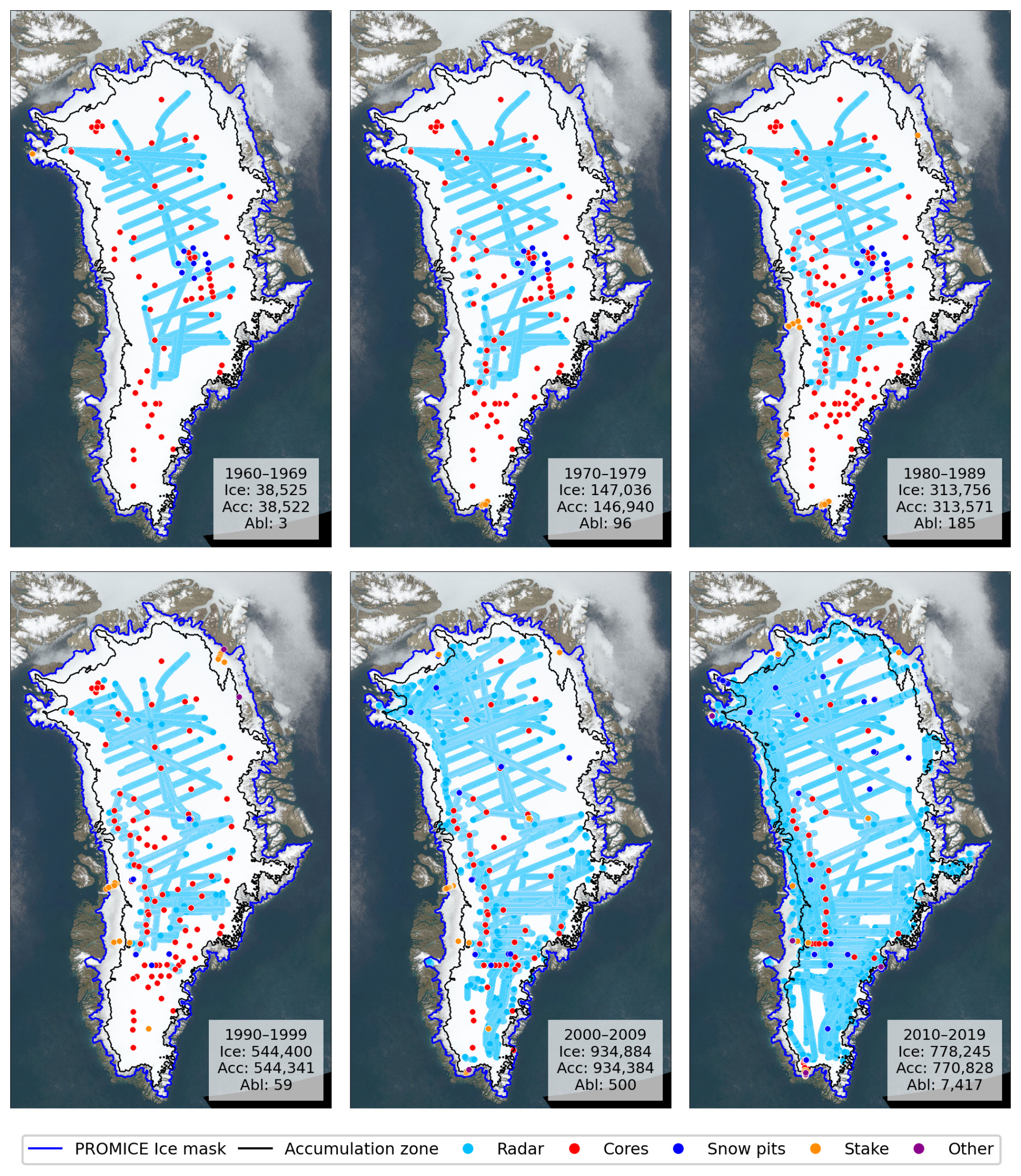
Figure A1 SUMup data distribution by decade, illustrated by measurement type. The method type “other” includes measurements from mass balance profile and SnowFox sensors. Values for “Ice”, “Acc” and “Abl” indicate the total number of data points for the ice-sheet, accumulation and ablation zones before radar grouping.

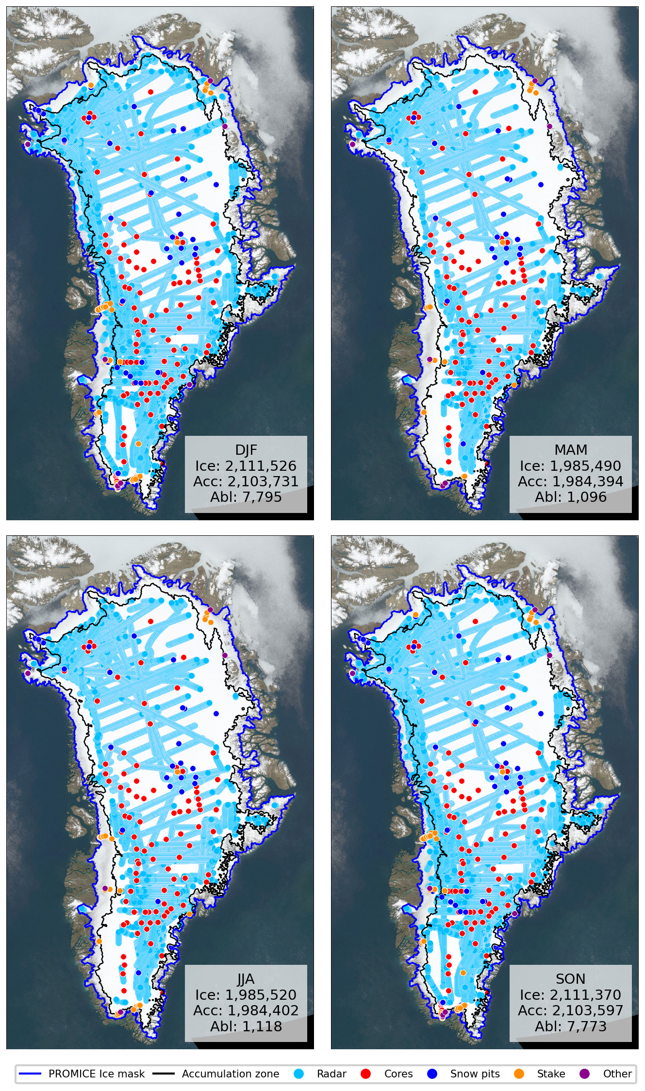
Figure A2 SUMup data distribution by season (1960–2022), illustrated by measurement type. The method type “other” includes measurements from mass balance profile and SnowFox sensors. Values for “Ice”, “Acc” and “Abl” indicate the total number of data points for the ice-sheet, accumulation and ablation zones before radar grouping.

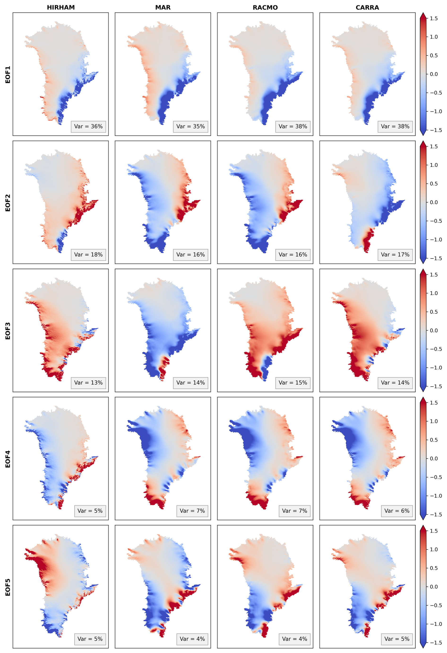
Figure A3 First five EOF patterns for HIRHAM, MAR, RACMO and CARRA over 1991–2022.

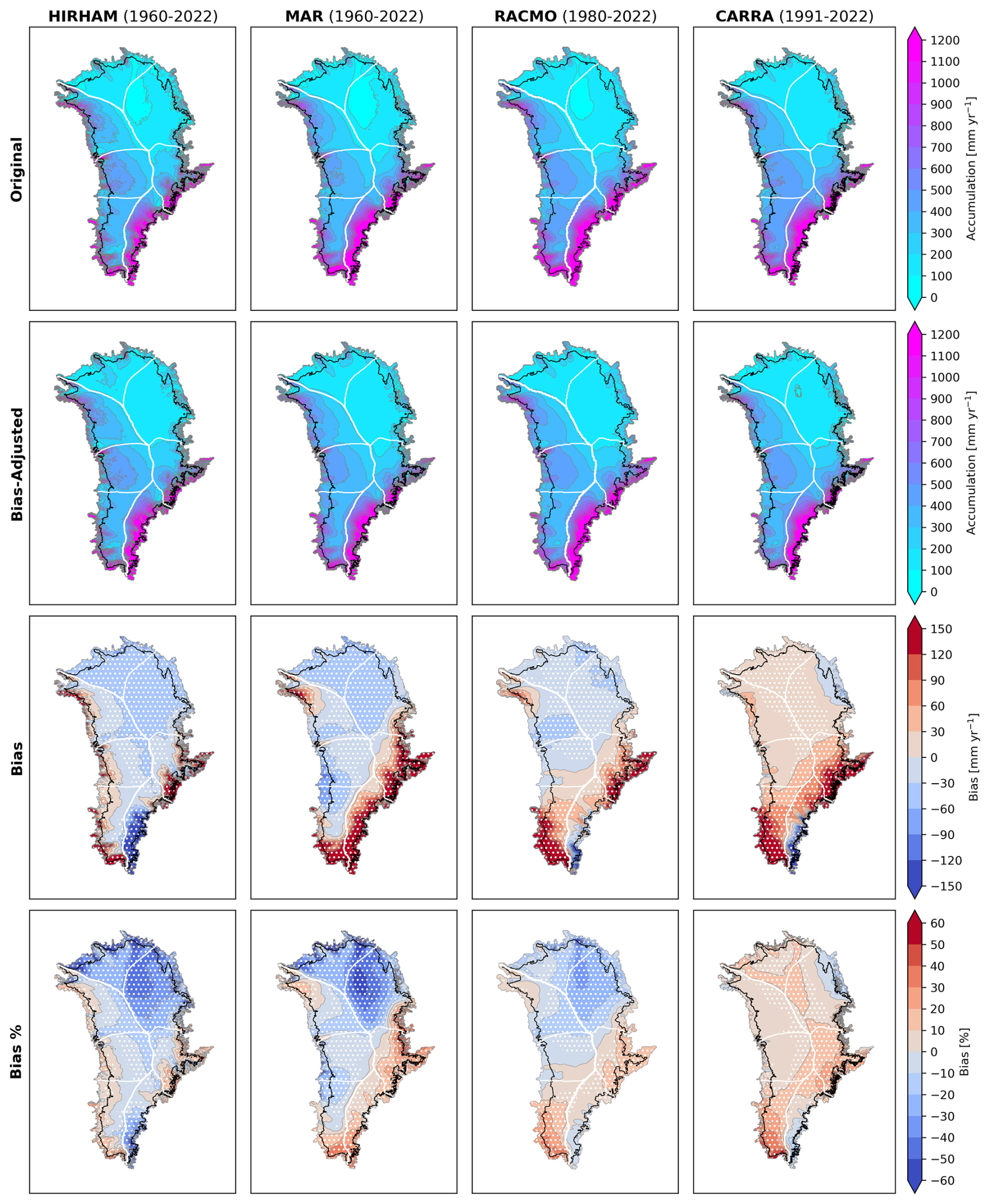
Figure A4 Mean maps of model accumulation and bias for the full model periods, HIRHAM (1960–2022), MAR (1960–2022), RACMO (1980–2022) and CARRA (1991–2022). The black line indicates the boundary of the accumulation zone. First row: original mean accumulation before adjustment. Second row: mean bias-corrected accumulation. Third row: mean bias in mm yr⁻¹. Fourth row: mean relative bias. Hatched regions indicate statistically significant biases (p<0.05). PROMICE drainage basin boundaries are indicated in white.

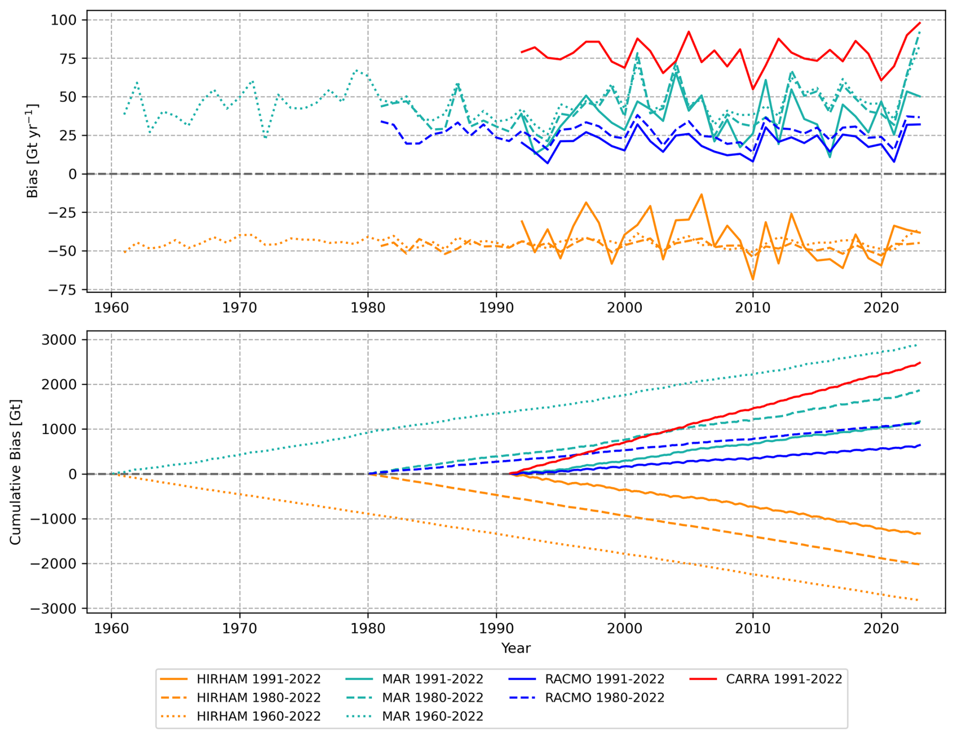
Figure A5 Spatially integrated annual bias for each model over the 1960–2022, 1980–2022 and 1991–2022 fitting periods, shown by year (upper) and as the cumulative sum (lower).

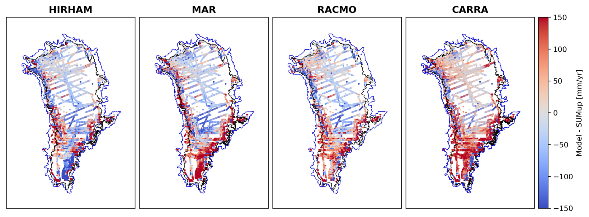
Figure A6 SUMup point-wise bias (1991–2022). The blue contour indicates the boundary of the PROMICE ice-sheet mask and the black contour shows the boundary of the accumulation zone.

A4 Appendix Tables

Table A1 Spatially integrated mean annual accumulation over the ice sheet, accumulation zone, and ablation zone expressed in Gt yr⁻¹ for original (Acc) and bias-adjusted (Acc_adj) accumulation. Net bias is defined as Acc − Acc_adj. Uncertainties for Acc_adj are obtained by Eq. (10). Statistically significant biases (p<0.05) are highlighted in bold.

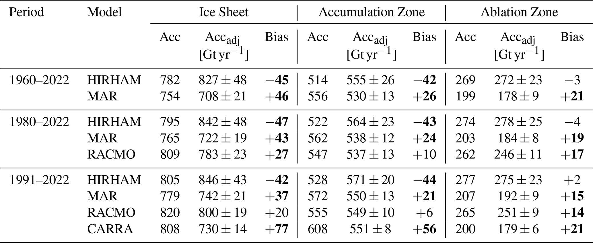
Table A2 Spatially integrated basin-wise accumulation net and relative bias expressed in Gt yr⁻¹. Bold values indicate statistically significant biases (p<0.05).

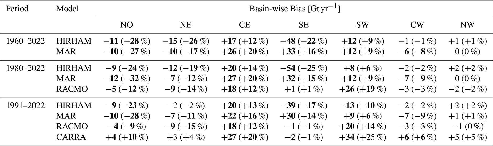
Table A3 Basin-wise accumulation trends in mm yr⁻¹ decade⁻¹, before/after bias-adjustment for each model and evaluation period. Values for each basin are shown before (left) and after (right) bias-adjustment.

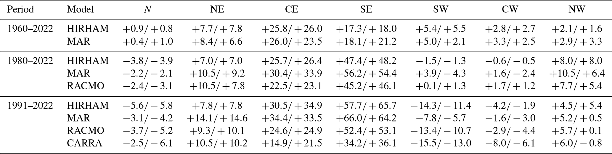
Table A4 Basin-wise spatial mean accumulation sensitivity to temperature (% K⁻¹) for each model and evaluation period. Values for each basin are shown before/after bias-adjustment.