Improving snow water equivalent modelling: a comparative study of hybrid machine learning techniques

Accurate characterization of snow water equivalent (SWE) is important for water resource management in large parts of the Northern Hemisphere, but its large spatio-temporal variability and limited observational data make it difficult to quantify. Complex physically-based models have been developed that allow long-term SWE simulation, but those still suffer from biases in their predictions, have long run times and provide challenges for integrating observational data. There have been recent attempts at using machine learning (ML) to improve SWE predictions from meteorological data with promising results, but the data scarcity issue and concerns about the ability to extrapolate in time and space remain. In this study, we evaluated two hybrid setups that integrate physically-based simulations and ML. The first setup, referred to as post-processing, follows a common approach in which the simulated outputs from a numerical snow model, Crocus, are used as predictors to the ML component in addition to the meteorological data. The second setup, named data-augmentation, involves an ML model trained not only on measured SWE but also on Crocus-simulated SWE at additional locations. These approaches were deployed using in-situ meteorological and SWE measurements available at ten stations throughout the Northern Hemisphere, and compared to Crocus and an ML setup using measured data only. The post processing setup outperformed all other approaches when predicting on left-out years in the training stations, but performed poorly when extrapolating to other locations compared to Crocus. The addition of a large set of Crocus-simulated variables besides SWE in this setup resulted in similar performance for left-out years but exacerbated the spatial extrapolation issue. On the other hand, the data-augmentation setup performed slightly worse on the left-out years, but showed much better transferability to new locations, improving the other ML-based setups greatly and reducing the RMSE in Crocus by more than 10 %. The feature importances of the ML-models were consistent with physical knowledge, despite having unusual deviations at extreme values, which showed some improvement for the data-augmentation setup. Lastly, the addition of lagged variables improved the results, but were only relevant for few variables and up to a week. These results prove the usefulness of hybrid models and particularly the data-augmentation setup for SWE prediction even in data-scarce domains, suggesting their potential to improve forecasts of SWE at large spatio-temporal scales, where they remain to be tested.

1 Introduction

The cryosphere has a large influence on landscapes and ecosystems globally, and its decline can have severe implications for human livelihood and economy (Huss et al., 2017). Snow, in particular, acts as a natural water reservoir, regulating seasonal runoff that impacts human socioeconomic activities both locally and downstream (Beniston et al., 2018; Biemans et al., 2019). Therefore, reliable estimates of snow water equivalent (SWE) are essential for accurate water resource assessment at various temporal and geographical scales. Nonetheless, important challenges remain for SWE quantification due to its spatio-temporal variability (Alonso-González et al., 2022; Deems et al., 2006; Grünewald et al., 2010). Considerable attention has been given to developing detailed land-surface and snow models for SWE and hydrological applications (e.g. Tarboton and Luce, 1996; Marks et al., 1999). Such models have also been used for avalanche forecasting, as is the case with Crocus, a complex physically-based snow model (Vionnet et al., 2012; Brun et al., 1989). When forced with reanalysis meteorological data, it has shown similar or better performance compared to other SWE products (Brun et al., 2013; Mortimer et al., 2020), but still exhibits significant discrepancies when compared to observed or field-derived snow conditions (Lafaysse et al., 2017; Menard et al., 2021).

During the last decades there has been a rapid increase in the application of machine learning (ML) models in hydrology, as they can improve the performance of traditional data-driven and physically-based modelling approaches thanks to their ability to automatically find both linear and non-linear structure in observed data and can easily adapt to multiple scales (Mosaffa et al., 2022). However, the success of such methods often depends on the availability of large, high-quality, standardized datasets, which are lacking in the case of SWE. Most previous attempts to estimate SWE with ML have relied on in situ snow depth measurements (Odry et al., 2020; Khosravi et al., 2023; Ntokas et al., 2021) or remote sensing data (Tedesco et al., 2004; Bair et al., 2018; Guo et al., 2003; Moradizadeh et al., 2023; Santi et al., 2022; Zheng et al., 2018; Song et al., 2024) as inputs. Hence, they are not suitable for prediction over long-time periods without snow data, i.e. for forecasting or for prediction at sites with null or limited observations. Nevertheless, recent studies have shown promising results when predicting daily SWE using only meteorological and static features (Duan et al., 2024; Wang et al., 2022).

A recent trend in scientific applications of ML is the combination with physically-based models (Reichstein et al., 2019). The resulting hybrid models may improve consistency with scientific knowledge, improving the accuracy and generalization of their predictions compared to purely data-driven approaches (Karpatne et al., 2017). Due to its easy implementation, one of the most common hybrid approaches is to use the outputs of a physically-based model as additional features to the ML model (Willard et al., 2022, Sect. 3.4.2). In this way, the ML algorithm is trained to minimize the error of the physically-based model relative to the observations. This “post-processing” approach has already been applied in the context of snow modelling. For instance, King et al. (2020) used a random forest to correct biases from a modelling and data assimilation SWE product in Ontario, and Steele et al. (2024) integrated outputs from a physically-based model into a hybrid LSTM framework to predict SWE and snow depth in several stations across the western US. However, no studies have comprehensively evaluated both temporal and spatial extrapolation capabilities of these type of models across diverse geographic regions for the purpose of SWE prediction. Alternatively, data-scarce problems such as SWE prediction may benefit from a hybrid approach that augments the training data using synthetic samples simulated with physically-based models. Nevertheless, while this modelling technique has obtained good results for other hydrological applications such as streamflow prediction (López-Chacón et al., 2023), its applicability in snow modelling remains unknown.

The primary objective of this study is to evaluate the suitability of hybrid models to predict point-observations of SWE from the meteorological time series at daily resolution over long time periods, i.e. several years or decades. In particular, we test the two previously introduced hybrid approaches, which will be referred to as post-processing (PPC) and data-augmentation (AUG). In situ snow and meteorological data from ten stations across the Northern Hemisphere are used together with snowpack simulations at the same locations using the Crocus snow model. The two hybrid approaches are compared to the SWE simulations run with Crocus and the outputs of a fully measurement-based ML model (MSB) on the same stations. The models are evaluated for (1) extrapolation to new years at stations for which historical SWE measurements are available, and (2) extrapolation to other sites where no SWE measurements have been used for model training. Furthermore, several aspects of model creation are explored, such as different ML algorithms and hyperparameters, as well as the incorporation of lagged or additional modelled state variables as inputs. Finally, the importance of the input features is examined to assess the physical plausibility of the ML predictions.

2 Data and methods

2.1 Measured SWE and meteorological data

The meteorological and SWE data used in this study corresponds to the ESM-SnowMIP meteorological and evaluation datasets, an international project that aimed to assess and compare snow modelling schemes (Krinner et al., 2018). The data was collected from ten stations throughout the Northern Hemisphere including seven to twenty years of in situ measurements. The availability of in situ SWE and meteorological data was prioritized over larger data sets with the aim of enabling the ML models to learn intrinsic snowpack processes rather than correcting the biases of a specific modelled meteorological input, which would limit the transferability of our findings. The choice of dataset is further discussed in Sect. 4.1.

The meteorological data was reported at hourly resolution and include the surface atmospheric pressure (Pa), the near-surface specific humidity (kg kg⁻¹), air temperature (K) and wind speed (m s⁻¹), the rainfall ($\mathrm{kg}{\mathrm{m}}^{-\mathrm{2}}{\mathrm{s}}^{-\mathrm{1}}$) and snowfall ($\mathrm{kg}{\mathrm{m}}^{-\mathrm{2}}{\mathrm{s}}^{-\mathrm{1}}$) rates, and the surface downward longwave (W m⁻²) and shortwave (W m⁻²) radiations. SWE (mm) was reported at varying time intervals depending on the station. For three of the stations automatic measurements from a snow pillow or cosmic ray sensor were provided at daily or hourly resolution, but for the remaining stations only manual observations were available at irregular intervals of one week or longer. These will be referred to as automatic and manual stations, respectively. As shown in Fig. 1, these stations cover distinct geographical areas of the Northern Hemisphere and elevations that range from sea level up to almost 4000 m. Besides that, they also encompass all snow categories described in Sturm and Liston (2021). A full description of the station characteristics can be found in Menard and Essery (2019).

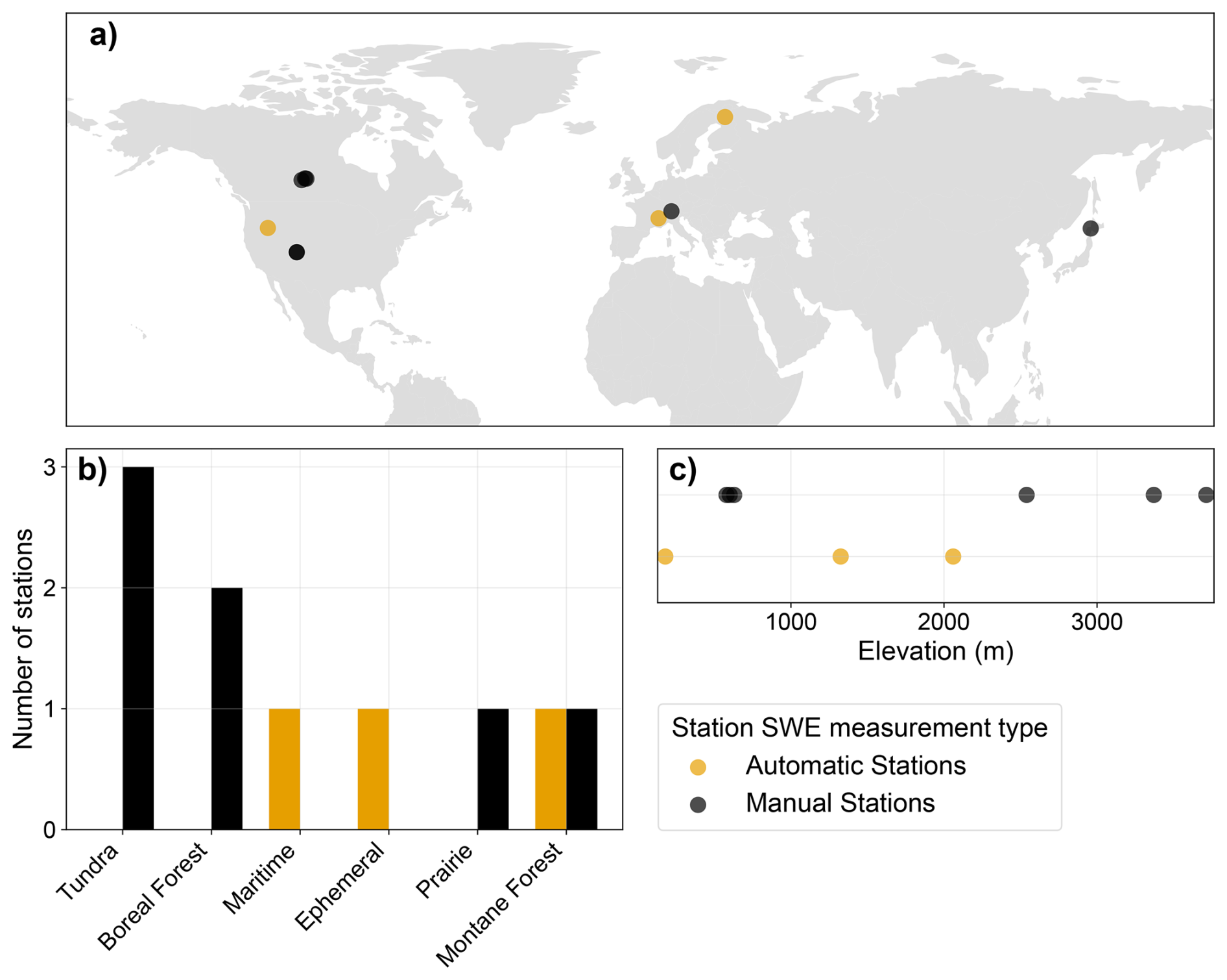
Figure 1 Characteristics of the ESM-SnowMIP stations including geographical location (a), snow category as defined by Sturm and Liston (2021) (b) and elevation (c) for stations with and without automatic daily measurements.

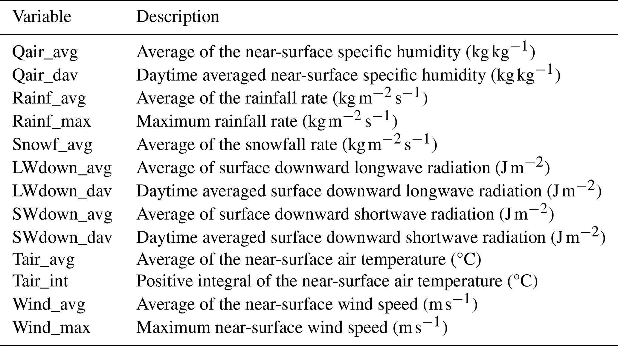
Because hourly SWE measurements were only available at a single station, all data was resampled to daily frequency, available instead at all three automatic stations. For the snow measurements, the value at 12:00 LT was selected to represent daily SWE, which corresponded to the hour at which most observations were available. For the meteorological variables, the daily value was calculated as the 24 h average (avg) in-between SWE measurements, capturing their overall central tendency throughout the day. For certain variables, aggregation methods other than the average were also applied, based on their role in snow dynamics according to expert knowledge. Specifically, the 24 h maximum (max) of the rainfall rate and wind speed, for which peak intensity plays an important role in snow melt and redistribution; the time integral (int) or sum of positive air temperatures in Celsius degrees, related to the wide-spread concept of degree-day factor (Hock, 2003) in melt modelling; and the average during daytime (dav) of the specific humidity, shortwave and longwave radiation, calculated as the mean of hourly observations between local dawn and dusk, therefore reducing their sensitivity to seasonal variations. The surface pressure was not used as a predictor since it was lacking observed data in some stations. The final daily aggregated meteorological variables fed to the ML models as input are described in Table 1.

Table 1 Description of daily-aggregated meteorological variables used as input for the machine learning models.

2.2 Crocus snowpack simulations

SWE and other snowpack variables coming from Crocus model simulations, generated for the ESM-SnowMIP project, were used in this study as part of the hybrid modelling approaches and as a benchmark for model evaluation. Crocus considers the energy and mass balance of the snowpack to model its evolution with high physical detail. It dynamically adjusts up to 50 snow layers to represent a vertically discretized snow temperature, density and liquid water content profile, and provides a comprehensive evolution of the snow microstructure, thus giving a vision of the snow stratigraphy and its temporal evolution. Crocus was forced with the aforementioned meteorological data to simulate a one-dimensional snowpack column at the ten ESM-SnowMIP stations with hourly resolution. The model was run without calibration and was coupled to the soil component of the land surface scheme ISBA (Vionnet et al., 2012), which tracks the temperature and moisture of 20 soil layers.

To conform to the daily frequency of the measured data, the Crocus-predicted SWE at 12:00 LT was selected for each date. Besides SWE, Crocus reports a range of bulk snowpack and individual snow layer variables. Specific snow layer variables were not directly used, but enabled the calculation of two additional bulk variables not reported in Crocus: the cold content, calculated as the sum of the layer-wise product of SWE, snow temperature, and specific heat of ice; and the snow bulk saturation, computed as the sum of the snow liquid content for all layers divided by the depth of the snowpack. All Crocus snowpack variables were resampled to daily frequency following the same procedure as the meteorological variables. Besides the averages, only the maximum daily surface temperature was added. However, for the snow depth and cold content, the value at the current time step (vcs) was considered more relevant than the average over 24 h, so it was used in its place. Lastly, information from the top soil layer was also retrieved and aggregated accordingly. The final aggregated Crocus variables are listed in Table 2.

Table 2 Description of daily-aggregated model state variables used as input for the machine learning models.

2.3 ML-based modelling setups

Besides Crocus, this study compared the performance of three modelling setups; an ML model purely based on measured meteorological data, and the two hybrid setups that integrate Crocus outputs into an ML framework, namely PPC and AUG. The models were designed to prognostically update the SWE state by conditioning on its value from the previous time step and the meteorological forcing, enabling their recursive application to generate long time series. A general overview of the three ML-based modelling setups is shown in Fig. 2.

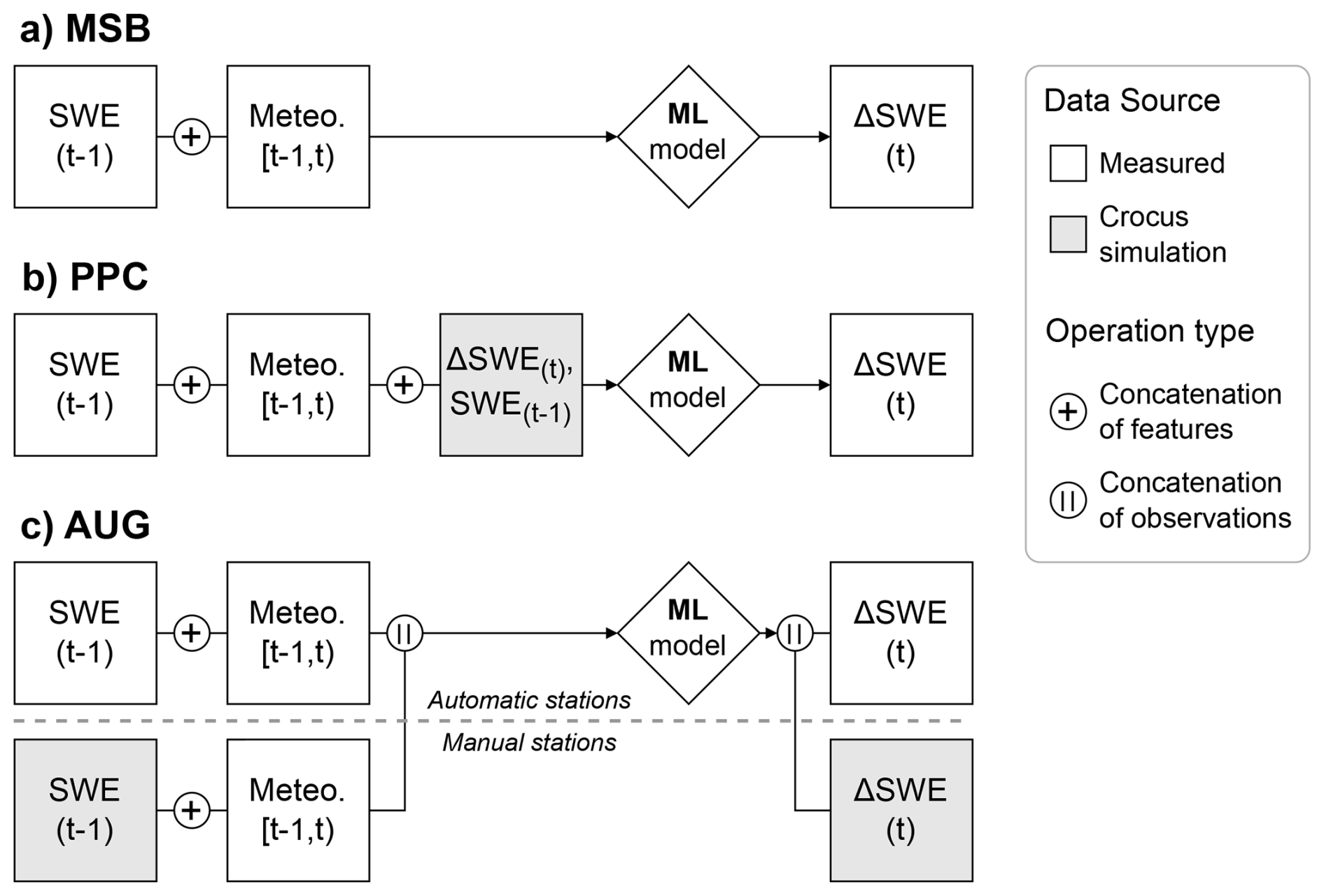
Figure 2 Diagram showcasing the training setups for the measurement-based (a), post-processing (b) and data-augmentation (c) approaches, where t represents the daily time step (at 12:00 LT), and $[t-\mathrm{1},t)$ the aggregated hourly data encompassing the 24 h period from 12:00 LT on the previous day to 12:00 LT on the current day, exclusive. All setups except AUG exclusively use data from the automatic stations for training. Concatenation of features refers to the inclusion of new predictors as input to the ML models, and concatenation of observations the integration of training points from different sources in their training.

2.3.1 Measurement-based ML model

The predictors in MSB were the SWE value at the previous time step and the daily-aggregated meteorological features, as defined in Fig. 2. To account for delayed snowpack responses to atmospheric conditions, the lagged meteorological variables for the previous 14 d were also included as predictors. In other words, the ML models were fed the meteorological data not only for the 24 h interval between the previous and current time step $[t-\mathrm{1},t)$, but also for the 14 preceding days, i.e. $[t-\mathrm{2},t-\mathrm{1})$, $[t-\mathrm{3},t-\mathrm{2})$, ⋯, $[t-\mathrm{15},t-\mathrm{14})$. The target of the ML model was the daily change in SWE, calculated as $\mathrm{\Delta }{\text{SWE}}_{\left(t\right)}={\text{SWE}}_{\left(t\right)}-{\text{SWE}}_{(t-\mathrm{1})}$. It should be noted that our approach limited model training to stations where consecutive daily SWE measurements are available, that is, the automatic stations. Furthermore, to avoid a bias towards zero in the predicted variable, measurements for which SWE_(t)=0 were removed. Ultimately, the number of available samples was 1874, corresponding to all consecutive SWE measurements excluding periods without snow or SWE changes that would result in a complete melt of the snowpack. Concerns regarding the small number of training samples are addressed in Sect. 4.1.

2.3.2 Post-processing hybrid model

In PPC, the physically-based model target is given as an input to the ML model together with the conventional predictor variables to produce a corrected or post-processed version of the target. In practice, this setup was implemented similarly to MSB, but the ML model was given two additional predictors at each time step: the daily ΔSWE retrieved from the Crocus simulations, the target to be post-processed; and the previous SWE value according to the Crocus simulations, to provide more context of the status of the Crocus-simulated snowpack to the ML model. The rationale is that the ML model can rely on the physical information of the snowpack stored in the Crocus simulations as a base for its predictions, correcting it when necessary based on the meteorological information. The addition of other Crocus state variables, namely the ones described in Table 2, was also tested but was not included in the main results due to poor performance (refer to Sect. 3.4.2).

2.3.3 Data-augmentation hybrid model

The AUG setup shares the same predictors with MSB, but the training dataset is augmented with synthetic observations. In our implementation, the Crocus simulations generated at the manual stations were used to provide synthetic SWE and ΔSWE training samples, filtered by following the same rules as for the measured data. This corresponded to an additional 18 717 observations. To balance the influence of the Crocus-generated data on ML model training, they were given a smaller weight in the loss function computed as the ratio of the number of measured to augmented training samples. There are two ways of interpreting this approach. First, as a measurement-based ML model that is implicitly regularized by adding model-generated data to guide its training. Second, as an ML surrogate of Crocus to which we incorporate SWE observations, but where the training for both observed and modelled data is performed simultaneously, simplifying the process.

2.4 ML Model selection and evaluation

Three different ML algorithms were tested: a random forest (RF), implemented with the scikit-learn library (version 1.3.0., Pedregosa et al., 2011), a feed forward neural network (NN) and a long-short term memory neural network (LSTM), implemented in the Keras library (version 2.12.0, Chollet et al., 2015). The LSTM enabled a sequential processing of the lagged daily-aggregated meteorological values rather than their inclusion as additional features, as with the other two algorithms. The hyperparameter combinations implemented in this study are described in Appendix A.

The process of ML model selection, training and evaluation followed the same general steps for the three ML-based modelling setups. First, the data was split into three sets: train, validation and test. A separate ML model was initialized for each algorithm and hyperparameter combination. Each model instance was fitted to the train set, and used for prediction in the validation set. Then, the best-performing model according to the mean squared error of ΔSWE was re-trained with both training and validation data, and used for prediction in the test set for a final evaluation. This process was independently applied to two data partitioning strategies, named temporal and station splits, which assessed model robustness when predicting at locations with and without historical SWE measurements in its training, respectively. By employing these distinct split types for each predictive goal and re-using the validation data before final evaluation, we optimized the efficient use of the limited available data.

In the temporal split, represented in Fig. 3a, a leave-one-out cross-validation strategy was used involving five contiguous folds of approximately 20 % of each station's data. Each fold began and ended roughly at the start of the hydro-year, ensuring that they contained at least one year of measured data. For each split in the cross-validation loop, a separate model was created that used three folds as train set, one for the validation set and one for the test set. In AUG, all models were also trained on the full time series of Crocus simulations at the seven manual stations during both model selection and evaluation. The station split, represented in Fig. 3b, again followed a leave-one-out cross-validation strategy, but in this case the train set consisted of the full time series from two of the automatic stations and the remaining station was used as validation set. The test set was comprised of all SWE data available at the seven manual stations. In AUG, an additional nested leave-one-out cross-validation loop was performed for each manual station to avoid evaluating the model on stations contained its training. So, the augmented data consisted only of six manual stations, and the remaining one constituted the test set, producing seven models corresponding to each cross-validation split.

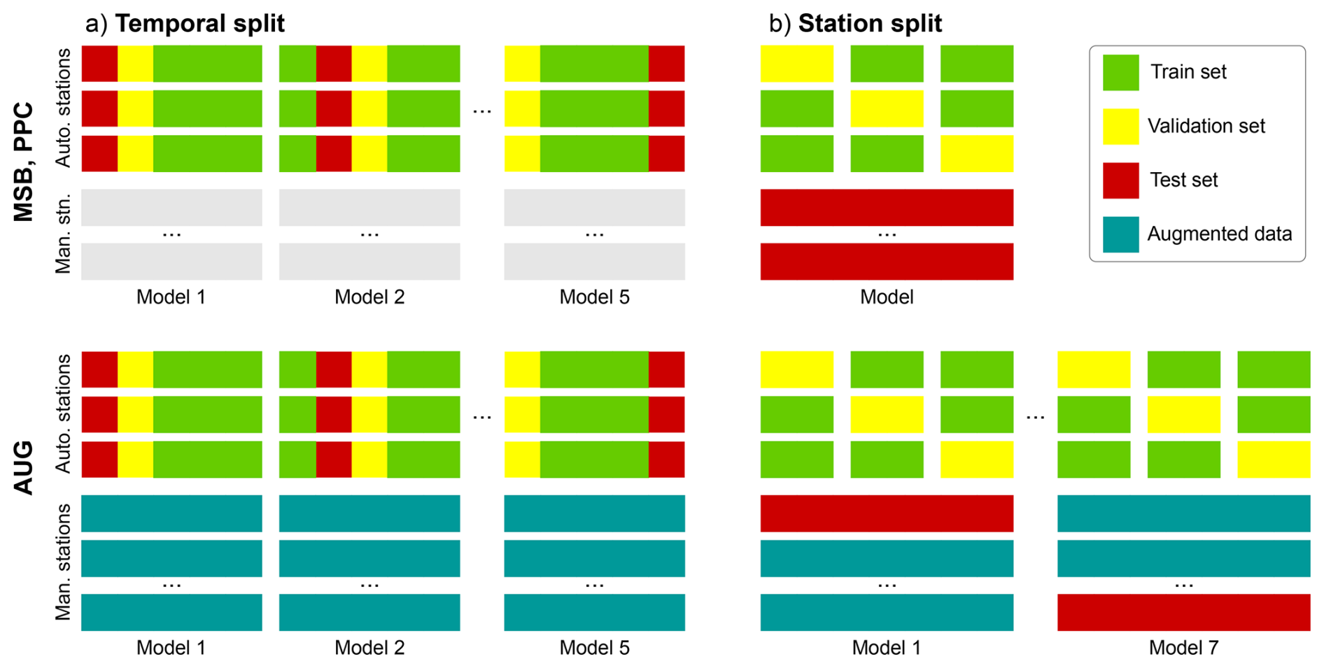
Figure 3 Diagram representing the train, validation and test sets used to select, train and evaluate the MSB, PPC and AUG models for the temporal (a) and station (b) split strategies. Each rectangle represents the full time series at a given station, the first three rows represent the automatic stations and the remaining ones the seven manual stations. The augmented data is also part of the training set, but uses the Crocus simulations instead of measured SWE data.

2.5 Analysis of SWE predictions

To evaluate the performance of the modelling setups for predicting SWE, the trained models were employed to generate a single time series of SWE for each modelling setup and station. First, an initial condition of SWE=0 was set at the starting date. Then, ΔSWE was predicted using the model whose test set encompasses that time step and station. Next, the predicted ΔSWE was added to the previous SWE, replacing any negative SWE values by zero. Lastly, the updated SWE value was stored and used as input for the subsequent date. This process was performed iteratively until input data was no longer available.

The data points for which measured SWE data was available were used to assess the model performance. The metrics computed for this study were the root mean squared error (RMSE), mean bias, and Nash–Sutcliffe efficiency (NSE), defined as one minus the ratio of the error variance of the model to the variance of the observed data. Furthermore, the feature importances were retrieved from each of the ML models for their test predictions using the SHAP library (Lundberg and Lee, 2017), which quantifies the contribution of each predictors to the deviations of the model output from its mean value for each time step.

3 Results

3.1 Optimal ML model configuration

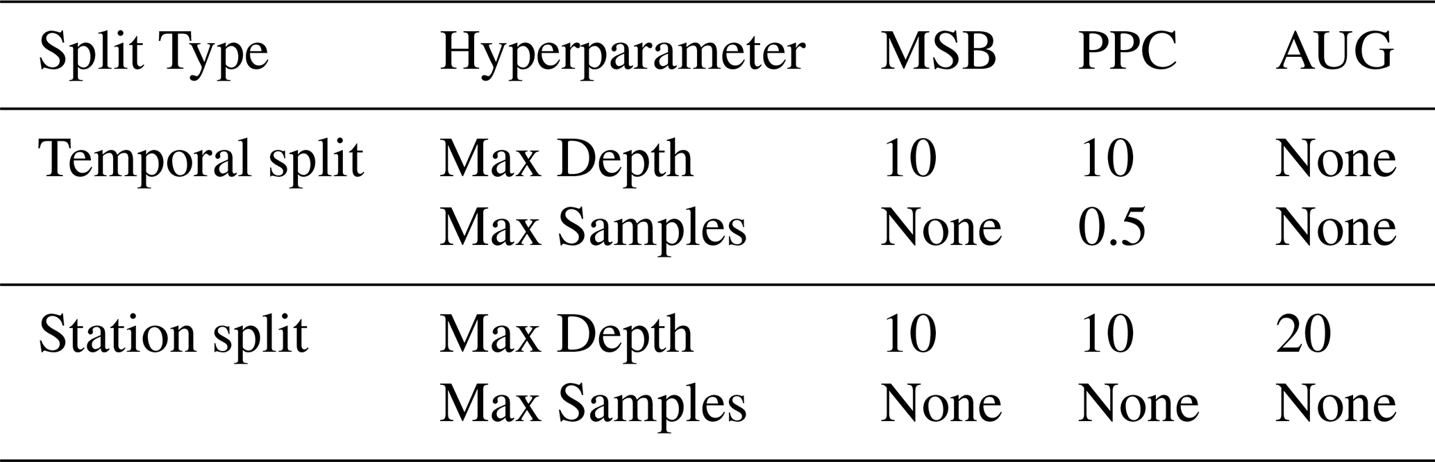
The results of model selection revealed the Random Forest algorithm to be consistently superior in all modelling setups. The NN and LSTM models attained 13 % and 23 % higher MSE values than RF on average, for all setups and splits. The differences in performance for different RF hyperparameters were not large, with differences below 5 % in MSE at the most. No clear positive or negative trend was found for any hyperparameter, besides generally getting slightly better results for larger values of the number of features. The hyperparameter configurations used for each modelling setup and split type are reported in Table 3. The other hyperparameters were left at their default value. For the remainder of this section, only the results from the best performing ML algorithm and hyperparameter combination for each setup are presented. Training was performed in under a minute for the RF models, using a single CPU core. Inference time for a single time step was on the order of magnitude of 50 ms. The results shown in the following sections used lagged meteorological variables, but without additional Crocus variables for PPC, which yielded the best performance. The impact of these two modelling choices is further elaborated in Sect. 3.4.

Table 3 Optimal Random Forest hyperparameter configurations for the different ML-based setups and split types.

3.2 Predicted SWE comparison

The test set NSE on the corresponding stations for each data split is displayed in Fig. 4 for all modelling setups. The most noticeable difference is the large gap in performance in all models between prediction on left-out years at the automatic stations and extrapolation to the manual stations. These correspond to the models trained and evaluated using the temporal and station data splits, respectively. In the temporal split, all models achieved similarly good performances, roughly between 0.85–0.95 test NSE. All ML-based setups outperformed Crocus, PPC achieving the highest score. AUG, however, failed to surpass the performance of MSB. Despite the success of the ML-based setups, they consistently underperformed Crocus at the two stations with smaller sample size. In the station split, all model performances decreased considerably, especially for MSB and PPC. These setups obtained a test NSE slightly below 0.70, but most stations remained below 0.3 and some even reached negative NSE values, indicating that the variation of the error was equal or larger than the variation in the observed data. In contrast, AUG attained the best performance with a test NSE of 0.85, even higher than the 0.80 of Crocus. Moreover, AUG exhibited the least performance variability across stations, none of them reaching below 0.46 NSE. In particular, AUG improves the NSE at 6 of the 7 test stations by an average of 0.27 compared to Crocus.

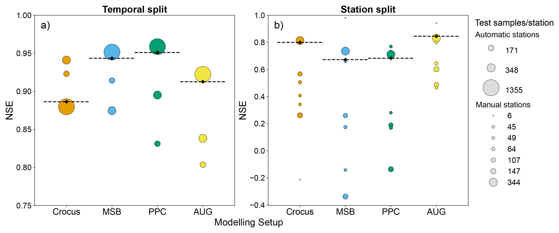
Figure 4 Bubble plots showing the NSE achieved by each modelling setup for predicting SWE for the temporal (a) and station (b) splits. The circles show the station-specific NSE, where the size corresponds to the number of test samples, and the dashed line indicates the NSE for the entire test set. Note the change in y axis scale between the two panels.

3.2.1 Time series of automatic stations

Figure 5 shows an example five-year subset of the SWE time series at one of the automatic stations. All four modelling approaches displayed good agreement with the observed snowpack dynamics; that is, the seasonal snow pattern was generally well reproduced. Moreover, they succeeded in capturing the variability in yearly peak SWE values reasonably well, with deviations of 10 %–15 % on average compared to the measured values. However, AUG and Crocus tended to underestimate the amount of snow. This argument is also supported by the mean bias at the test stations (Appendix B), which was more than two times smaller for MSB and PPC than for the other setups. Because of this, the peak SWE values were also underestimated, especially by Crocus. Another noticeable pattern was the increase in absolute error of the predicted SWE as the snow cover period advances. Importantly, a large spike in the residuals was observed at the last part of the snow ablation period due to the inability of the models to accurately reproduce its exact timing. Once more, this effect was most pronounced in Crocus, which predicted the full melt almost 6 d earlier than measured, on average. Conversely, the ML-based counterparts exhibited only a slightly positive shift in the snowpack melt-out date, most pronounced in the PPC mode, which resulted in smaller error overall.

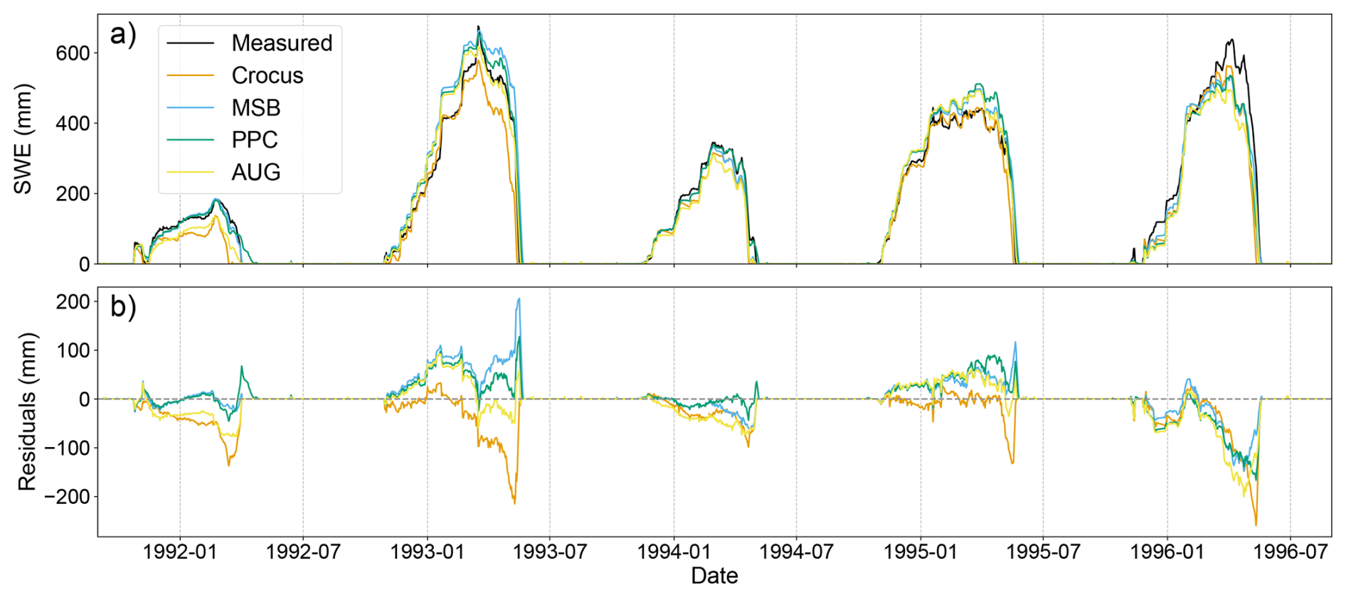
Figure 5 Time series for an example five-year range in the Reynold Mountain East station, the automatic station with most available samples, showing the SWE time series (a) and the corresponding residuals (b) from the measured data, Crocus SWE simulations, and predicted by the ML-based setups trained with the temporal split.

3.2.2 Time series of manual stations

To compare the predicted SWE time series of the models trained with the station split, Fig. 6 shows a five-year fragment from the manual station with most available samples. It is important to note that the models had much larger variability in performance between stations and years, making it difficult to find a subset that represents the whole test set well. The first noticeable characteristic is a much poorer fit, relative to the predictions in automatic stations. In particular, the residuals grow significantly after the main snow accumulation phase due to a large underestimation of SWE. This bias had a considerable effect on the peak SWE values, which have a more than 100 mm deficit on average for MSB and PPC and around 80 mm for AUG. While Crocus still had large absolute errors in peak SWE prediction, it could predict it with much fewer bias, around 25 mm. This trend was also reflected in a large increase of the test mean bias for the ML-based setups compared to the automatic station predictions (Appendix B), which obtained much larger values than Crocus, especially MSB and PPC. However, AUG had less absolute mean bias for the majority of the stations, and improved by more than 10 % its test RMSE. Notably, AUG managed to predict the snow ablation much better than any other setup, achieving lower residuals in the last few snow measurements for each snow year in almost all instances displayed in Fig. 6, and more generally across all stations and years with sufficient available measurements.

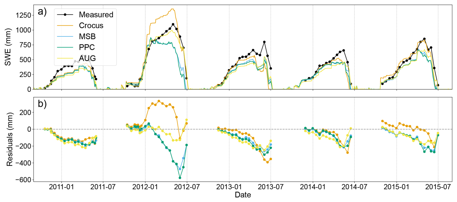
Figure 6 Time series of a five-year range in the Weissfluhjoch station, the manual station with most available samples, showing the SWE time series (a) and the corresponding residuals (b) from the measured data, Crocus SWE simulations, and predicted by the ML-based setups trained with the station split. Because of the large portion of missing data, the measured SWE and derived errors are displayed with dots connected by line segments for better visibility.

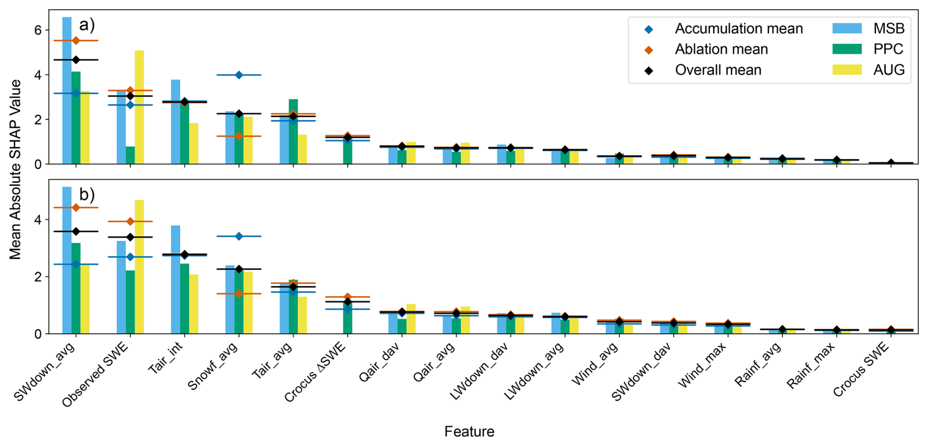
Figure 7 Feature importances of the input variables (defined in Table 1) of the ML-based models, defined as their mean SHAP absolute value, for the temporal (a) and station (b) splits. The bars represent the importances from each specific modelling setup, and the line and diamond combinations, their average. The latter are also shown for the accumulation and ablation periods, defined according to the sign of the predicted ΔSWE.

3.3 Feature importance of the ML-based models

According to the results of the SHAP analysis for both data split types (Fig. 7), the most important variable for most setups, and particularly for MSB, was the averaged downward shortwave radiation. This variable is not only indicative of snow melt, but also strongly related to seasonality, which may explain its high importance throughout the whole snow period. The observed SWE obtained the second largest mean value across the ML models, which is reasonable since this is the only variable which contains direct information on the state of the snowpack. Interestingly, PPC gave very little importance to this variable in the temporal split, despite obtaining the best performance. Both variables derived from air temperature, but especially the sum of positive values, were amongst the three most important features, indicating that the energy balance highly influences the predictions of the models. The snowfall also featured in the top five variables as the strongest positively correlated variable with ΔSWE. For more information about the correlations between each variable and the target refer to Appendix C. Beyond this, PPC gave a marked importance to the change in SWE simulated by Crocus, which ranked 5th and 6th in terms of feature importance in the temporal and station splits, respectively. This shows that the modelled target is indeed a valuable variable for predicting SWE, although far from the most important. Other variables that were considered moderately important include those derived from air humidity and downward longwave radiation. Finally, the variables related to rainfall and the Crocus-simulated SWE were the least impactful in the model predictions.

The SHAP analysis for the temporal (Fig. 7a) and station (Fig. 7b) splits share many similarities. Indeed, the top five most important variables were exactly the same. However, there were some interesting changes. The most noticeable was a substantial increase in the importance of the observed SWE in PPC for the station split, and less importance given to the short-wave radiation compared to the other variables. The differences between the accumulation and ablation periods, defined as the time steps for which the predicted ΔSWE is positive or negative, were also analysed. As expected, in the accumulation period the snowfall rate became the most important variable, with a substantial increase compared to the overall results. Moreover, the shortwave radiation and temperature variables became less important. An opposite trend could be observed for the ablation period, where the snowfall rate became less important in favour of the shortwave radiation and air temperature, but not enough to substantially change the order of the feature importances. Lastly, the Crocus-simulated ΔSWE was more important in the ablation period than in the accumulation period, especially in the spatial split.

The ML models were able to capture some expected physical relationships, such as negative correlation with the air temperature and shortwave radiation and a positive one with snowfall. Moreover, when predicting on the training stations with the temporal split (Fig. 8a–c) the snowfall rate was found to have the expected linear relationship with the predicted output. There was only some bias for higher snowfall values, which was corrected in AUG. Nevertheless, for the ML-based models tested using the station split (Fig. 8d–f), this bias was even more evident. So, while there was still a clear linear relationship between SHAP and observed snowfall for low to mid values, above a threshold of approximately 0.7 $\mathrm{g}{\mathrm{m}}^{-\mathrm{2}}{\mathrm{s}}^{-\mathrm{1}}$, any additional snowfall did not result in a further increment of SWE. This indicates that the ML models could not extrapolate to stations with higher snowfall events, and underpredicted these extreme cases.

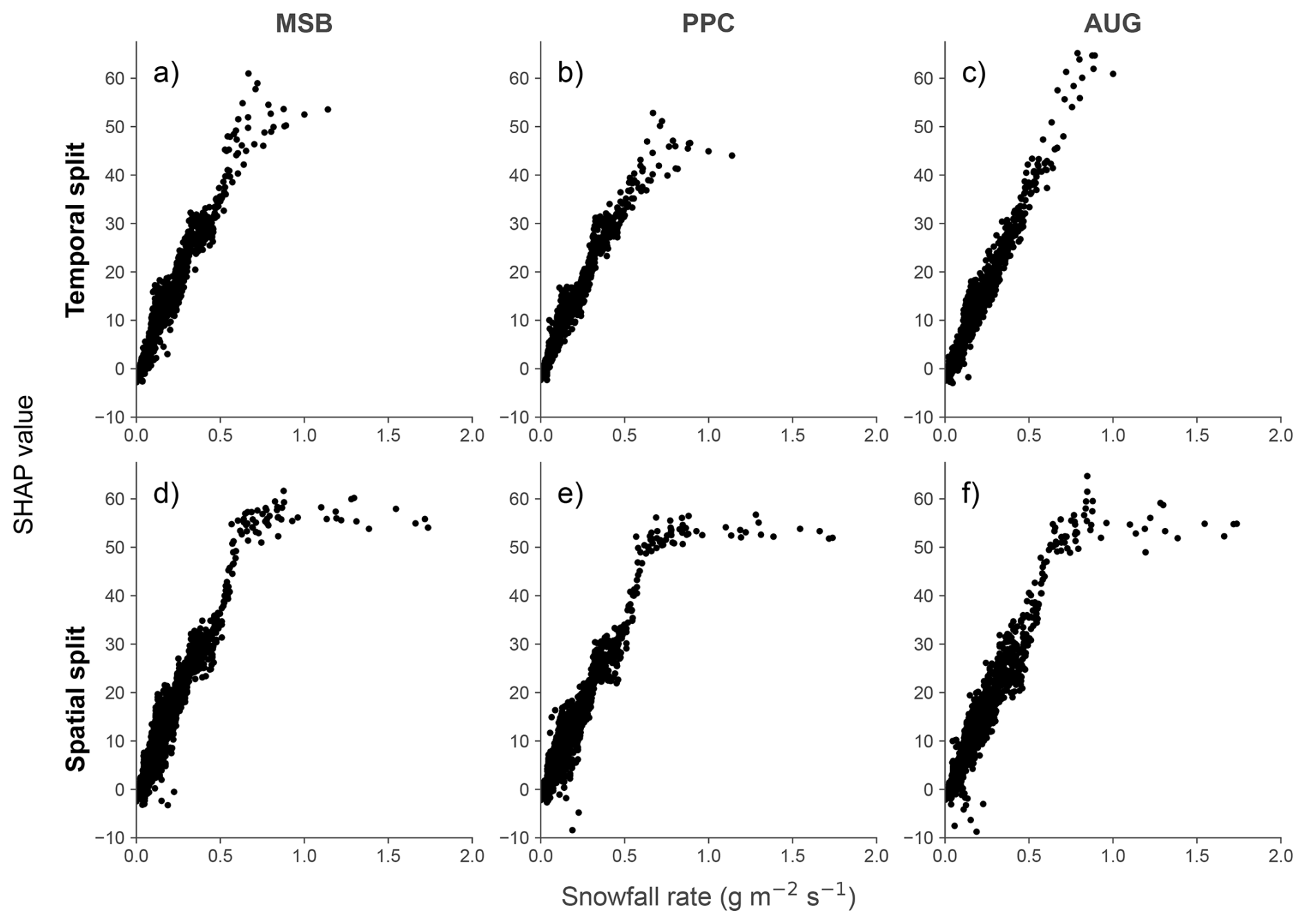
Figure 8 Scatter plot of the SHAP values against measured values of the daily averaged snowfall rate. The SHAP values quantify the deviation in the predicted ΔSWE from its average value over the test samples, as caused by the specific value of the snowfall rate in each of them. The three ML-based setups are compared for both temporal (a–c) and spatial (d–f) data splits.

3.4 Impact of modelling choices

3.4.1 Addition of lagged features

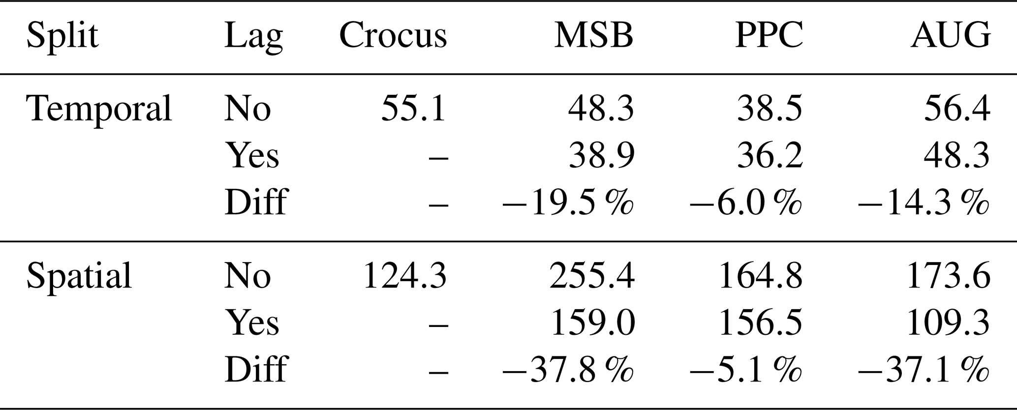
The impact of adding lagged meteorological information in the ML-based model inputs was tested by comparing the results in which the ML models were given the previous 14 d of meteorological information as additional inputs against the same models without any lagged variables. The reported RMSE of both and the improvement from one to the other is shown in Table 4. The RMSE obtained with Crocus is shown as well for reference. In the temporal split, the lagged version reduced the error of MSB and AUG considerably, while PPC achieved similar results. For the station split, a similar pattern is observed. This time the decrease in RMSE for MSB and AUG was even larger, roughly 37 %, while for PPC it remained around 5 %. Hence, having Crocus-simulated variables as input made the model much less dependent on past information to obtain good performance, which becomes especially relevant when predicting on new stations. The reason may be that the Crocus predictors already implicitly included the memory of the past days.

Table 4 Comparison of RMSE values for each setup and split with and without adding lagged variables, and the percentage difference (Diff) between them.

Moreover, the importance of the added lagged features was explored through an analysis of their SHAP values. Figure 9 shows the mean absolute SHAP value of the 14 lagged values for the three most influential meteorological variables, determined in Sect. 3.3. In general, feature importance decayed very quickly for larger lag values, but there was some distinction between features. The shortwave radiation had the slowest decrease in importance, with some of the lagged inputs within the preceding week having a noticeable effect. For AUG in particular, the relevant lagged window was further reduced to 3 d. For the air temperature, only the value at the day before had a relevant impact, which was mostly null for larger lagged values. Lastly, the snowfall rate of any of the previous days had little to no impact on the model predictions. In conclusion, the addition of lagged meteorological variables was not relevant for more than a week before, and in some cases markedly less.

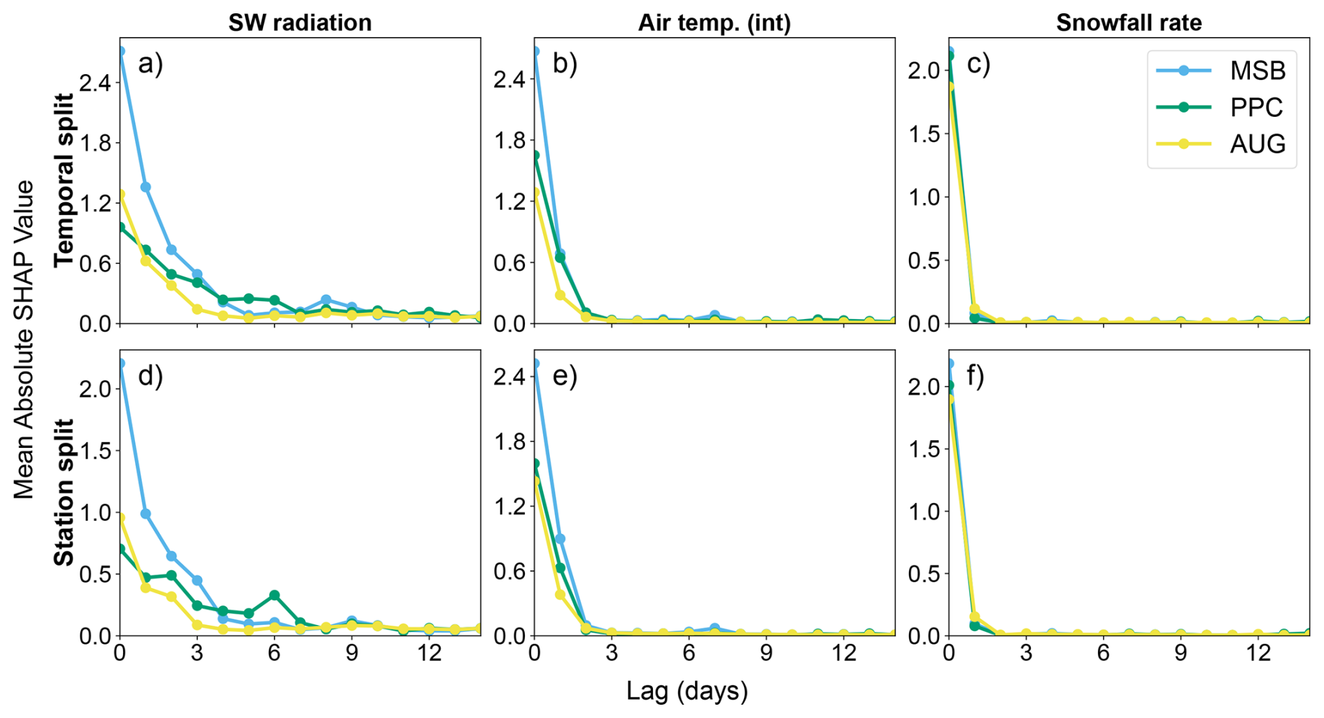
Figure 9 Feature importance of the 14 historical values of the three most influential meteorological variables for the temporal (a–c) and station (d–f) splits.

3.4.2 Addition of Crocus state variables

Another goal was to determine the usefulness of incorporating additional Crocus state variables besides SWE and ΔSWE in PPC. To do so, another model named PPC-enriched was trained similarly to PPC but also including the variables defined in Table 2 as inputs. The hypothesis was that by providing additional context on the state of the modelled snowpack, the ML component may improve its ability to correct Crocus predictions. When trained with the temporal split, PPC-enriched achieved an NSE of 0.95, the same as the regular PPC. Hence, despite the good performance, the simpler model was favoured for the general analysis. Furthermore, for the station split, the NSE dropped to 0.20, substantially lower than any of the other setups. In four out of seven test stations it yielded negative NSE values of up to −3.00. When investigating the feature importances of PPC-enriched, the main difference amongst the most influential variables was a replacement of the downward shortwave radiation by the Crocus-reported average net radiation, which might not generalize as well to other stations. In conclusion, the overall effect of adding additional Crocus state variables was neutral or negative, discouraging the use of PPC-enriched.

4 Discussion

The results of the study show that hybrid models can outperform both state-of-the-art numerical snow models and classic ML approaches for SWE simulation at point locations, based on meteorological data. However, the optimal type of hybrid setup highly depends on the intended use of the model.

When predicting at locations for which historical SWE measurements are available for model training, all ML-based models outperformed Crocus. These results are in line with recent literature in ML for hydrology, which has been found to outperform traditional numerical models in a variety of tasks (Mosaffa et al., 2022). The differences in performance concentrated towards the end of the snow period, where the ML-based models showed an improved timing of the snow melt. This disparity points towards an opportunity to further refine the characterization of melt dynamics within Crocus. The setup that achieved the best performance in all metrics computed for this study was PPC. The improvement of this type of hybrid setup over traditional ML approaches for SWE prediction coincides with the findings of Steele et al. (2024), who demonstrated that a similar strategy outperformed a purely ML counterpart, as well as other statistical and physically-based models, for predicting SWE and snow density using similar predictors. On the other hand, the low performance of AUG compared to the other ML-based setups indicates limited transferability of the snow dynamics between the manual stations (simulated with Crocus) and the automatic ones, favouring models specialized in the latter such as MSB and PPC. Finally, all ML models did capture expected correlations between ΔSWE and its predictors. For instance, downward short-wave radiation and air temperature were amongst the most influential variables dominating snow melt, and there was a clear positive linear correlation between snowfall and increase in SWE. This indicates that such models are able to correctly identify physical patterns in the data when the training data is sufficiently representative of the application domain. However, some variables such as downward shortwave radiation may show higher importances than expected, likely due to their role as indicators of seasonality.

When predicting on new locations not present in model training, the performances of all setups were lower and had larger variability than in the temporal split. This higher difficulty to predict in different sites is likely related to the small number of stations used in this study and the lack of predictors for spatial variation, such as the topography at the sites. For Crocus, which does not rely on any training or calibration, this decrease in performance could be caused by biases in the choices made during model creation. Col de Porte, one of the automatic stations, has historically been used for its development (Brun et al., 1989, 1992), so it is expected that it would have better performance in this or other stations featuring similar dominant snow processes. MSB achieved the worst performance, mostly due to a strong negative bias. These results are consistent with a well known limitation of ML models, namely their need for large, representative datasets (Xu and Liang, 2021). PPC obtained similarly poor results, indicating that the corrections learnt by this type of hybrid setups do not generalize well to other sites. Conversely, AUG achieved the best results, even improving Crocus RMSE by more than 10 % and reaching higher NSE at all but one station, although it did exhibit a larger bias. Its large improvement over the other ML-based approaches could be attributed to Crocus being able to make better prognostic predictions out of sample due to its grounding in well-established physical equations, so the ML model in AUG is able to transfer its knowledge when predicting in stations with similar meteorological conditions. Nonetheless, the ML-based models evaluated on the station split exhibited anomalies in how certain input variables influenced their predictions. For instance, the predicted increase of SWE preserved the linear behaviour with snowfall for mid to low values, but saturated after a certain snowfall value was surpassed. However, AUG could extrapolate slightly further than the other setups, which indicates that targetting more extreme meteorological conditions in the augmented data could reduce this type of anomalies.

An analysis on the importance of lagged variables showed that their addition substantially improved the results for most methods except for PPC, which displayed only minor improvements. This could be expected given that Crocus already digests the information from the previous meteorological conditions affecting the snowpack, hence its output already contains lagged information implicitly that the ML model can exploit. Nevertheless, the importance of the lagged variables rapidly decayed with the number of lagged days and was essentially null after a week, which suggests that longer lag times may not be needed. Incorporating lag was most impactful for the downward shortwave radiation, likely in link with snowpack warming and ripening prior to melt and for capturing the seasonal pattern. Future studies that cover even longer lag windows or evaluate the sensitivity of site conditions to the importance of lagged variables would be highly beneficial. An additional experiment was performed to investigate the effect of introducing Crocus state variables as additional predictors to the PPC setup, which resulted in little improvement in the temporal split and a large performance loss for the station split. The latter seems to be caused by an over-fitting of Crocus variables such as its reported net radiation, which might not be as generalizable to other stations as the measured radiation variables. These results emphasize the need for a larger training dataset representative of all snow climates if further modelled snow variables are to be exploited with a view of a large generalization capability. Moreover, for applications at regional scale, variable selection should be based on an understanding of snow climates and other sources of spatial heterogeneity of the region of interest. Further research in the selection and refinement of predictor variables and their aggregation methods for this type of models remains a promising area for study.

4.1 Limitations and recommendations

The main limitation of this study was the small number of measured locations. The choice of this data set was motivated by the high quality of the data, consisting of in-situ SWE and a significant number of meteorological variables measured for 7 to 20 years, and the diversity in site characteristics. However, it means only ten stations were available, of which only three had daily SWE measurements. This highlights the need for standardized SWE datasets relying on direct measurements, which are currently few in number and small in scope. The small number of training stations was especially limiting for prediction in the station split, which might have magnified the success of AUG, and restricts our results to the climates and site characteristics covered by this dataset. Additional research on larger datasets that cover different snow climates would be recommended to provide a complete assessment of the methods described in this paper. Another important point is the known errors of the SWE and meteorological datasets, acknowledged in Ménard et al. (2019). Given the data limitations, deviations in the data could become especially relevant and this study did not quantify the uncertainties of the SWE predictions.

A crucial improvement of the AUG setup over Crocus and other similar physically-based models is its shorter inference time. As such, it is particularly relevant for large or global scale SWE prediction. Moreover, Crocus requires a detailed set of meteorological variables that may not be available at larger scales or for future scenarios, whereas the ML-based nature of this approach enables adjusting to any available predictors. On the other hand, PPC is expected to improve its performance compared to AUG when trained on larger datasets, since it would broaden the interpolation range of the model. Furthermore, this setup reduces training time, but requires running the physically-based model on both training and inference station-years. Therefore, testing simpler and faster physically-based models to be used for this setup would be highly relevant in future studies. Hybrid setups similar to PPC show promise not only as competitors to physically-based models but could also be aimed at improving them, for example by finding which type of variables are better at explaining biases in the models, and for which conditions those are largest.

Larger training sizes could also affect the optimal choice of ML algorithm, instead of the current RF. For example, other studies have shown that LSTMs can result in enhanced SWE simulations when using larger datasets (Steele et al., 2024; Duan et al., 2024; Cui et al., 2023; Song et al., 2024). Such models usually require more extensive hyperparameter tuning, which was given a limited computational budget in this study. Furthermore, an implementation of LSTM that could extend beyond the 14 d window, or similar ML algorithms such as Gated Recurrent Units (Cho et al., 2014), could prove very valuable for snow modelling. Finally, further testing of these hybrid setups using modelled meteorological data, required for forecasting applications, is necessary to provide an estimate of their expected accuracy in an operational environment, where performance is likely to degrade.

5 Conclusions

This study tested two hybrid ML approaches compared to a baseline ML and physically-based approaches for long-term prediction of daily SWE based only on meteorological data both in left-out years from the training stations and in independent test stations. The more commonly used PPC setup outperformed both Crocus and the other ML-based approaches for predicting in left-out years, suggesting that ML models can benefit from additional model-simulated information. However, when tested on the independent stations, this setup performed markedly worse than Crocus, indicating that the knowledge gained in the training stations could not be generalized to other locations. Adding more Crocus-based features besides the target did not improve the model and impaired its generalization capabilities, warning against indiscriminately adding model-generated variables as predictors for applications with limited data. The addition of lagged variables, on the other hand, proved beneficial for model performance. The AUG approach, a novel hybrid setup in the context of SWE prediction, failed to improve the other ML models for predicting in left-out years at the training stations but excelled at prediction in new, untrained locations. There, it not only substantially improved the results from other ML-based approaches, but also reduced the RMSE from Crocus by more than 10 %. These results demonstrate that hybrid models, AUG in particular, have the potential to produce detailed long-term SWE predictions that generalize well to unseen conditions by using physically-based model simulations to complement the information provided by observed data. Nevertheless, further validation using modelled meteorological datasets is required to enable their use for prediction at large geographical extents.

Appendix A: ML hyperparameter choices

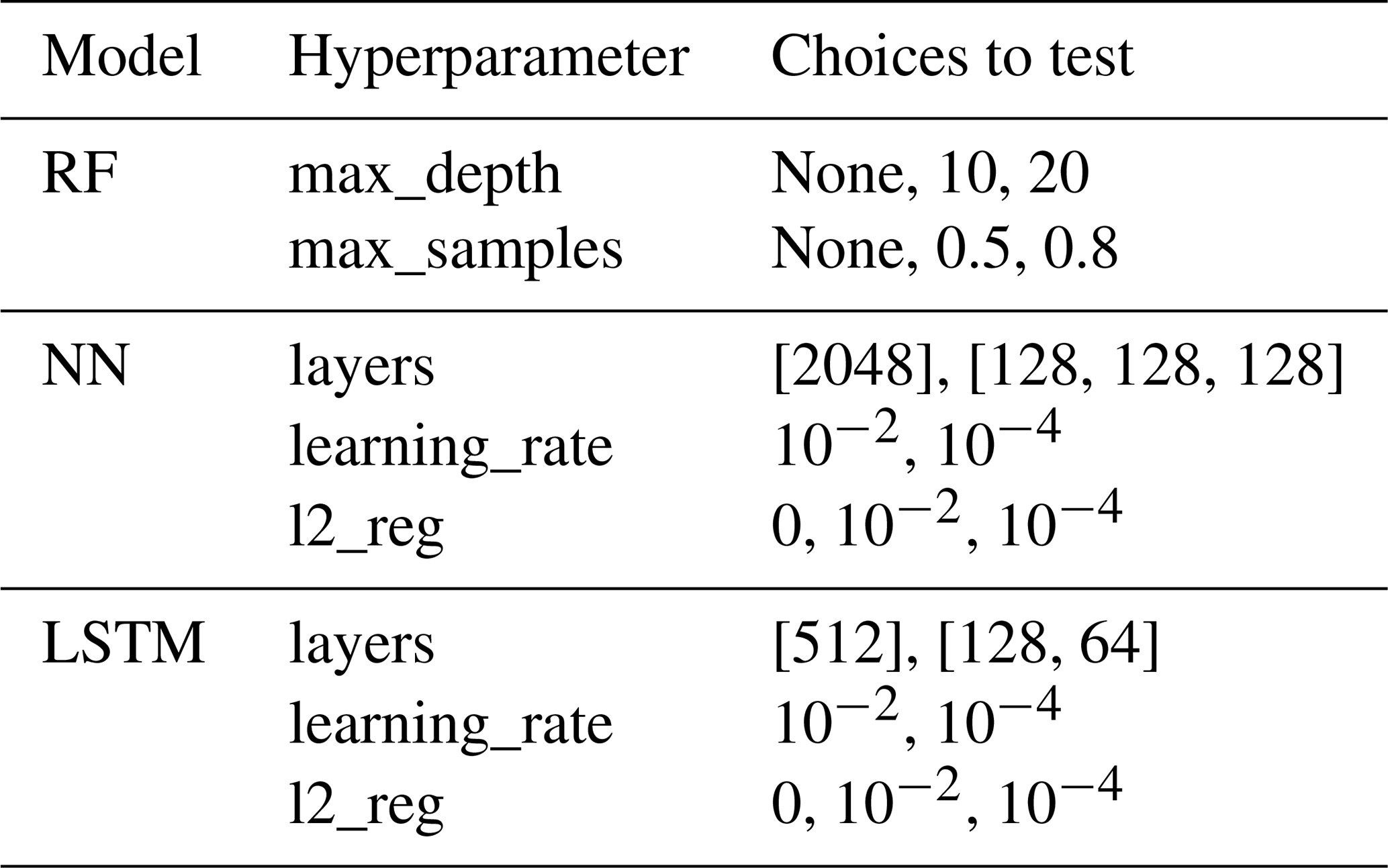
Three model types are explored in this study: random forest (RF), fully connected neural networks (NN) and long-short term memory (LSTM). The different hyperparameters tested for each of them can be found in Table A1. For RF, two parameters are tuned: the maximum depth of the trees that conform the RF algorithm (max_depth), which allows to find the right balance between bias and variance; and the subsample size for each tree (max_samples), which allows to find the right balance between stability and diversity of the trees. For both NN and LSTM models, three parameters were tuned: the number of layers and their units (layers), covering a a simpler and a more complex architecture; the learning rate (learning_rate), which determines the step size during weight optimization, crucial for converging to a global minimum; and the strength of the L2 regularization (l2_reg), aimed at preventing overfitting and improving the generalization of the models.

Table A1 Model types and hyperparameter choices that are compared for each setup.

Appendix B: Results of additional metrics

The performance of the models according to their NSE, RMSE and mean bias for both temporal and station splits is reported in Table B1.

Table B1 Model performance metrics across different stations and the full test set for temporal and station splits.

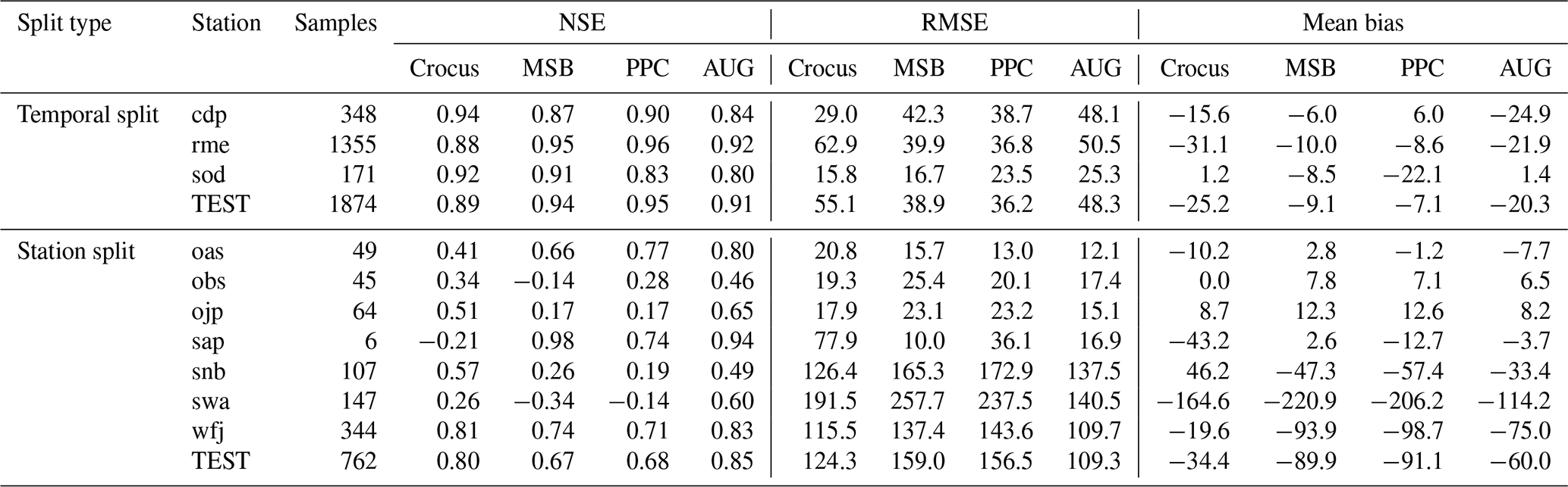
NSE: Nash–Sutcliffe efficiency, RMSE: root mean square error in $\mathrm{mm}\mathrm{w}.\mathrm{e}.$

Appendix C: Detailed SHAP analysis

Figure C1 provides information on the distribution of SHAP values over all test time steps for the five most important variables for each split type and model setup. For example, while on average the snowfall is not necessarily the most important variable, for specific time steps with high snowfall rates it has the strongest influence on the model output by almost an order of magnitude. Similarly, the ΔSWE predicted by Crocus barely features amongst the most important variables for PPC on average, but for some steps it very strongly influences the decrease in SWE. The influence of other variables, such as air temperature or shortwave radiation, is less extreme for a single time step. They have a positive impact distributed over many time time steps when their values are low, but also show a stronger negative influence but in a smaller subset of time steps when their values are high. Finally the observed SWE shows a bimodal distribution that indicates that it has a strong influence in both the increase and decrease of SWE, for low and high values respectively. Very low SWE values had a positive effect on the predicted ΔSWE, but otherwise its net effect was negative. The impact of this variable fluctuated greatly, though, showing the strongest interaction effect with the air temperature.

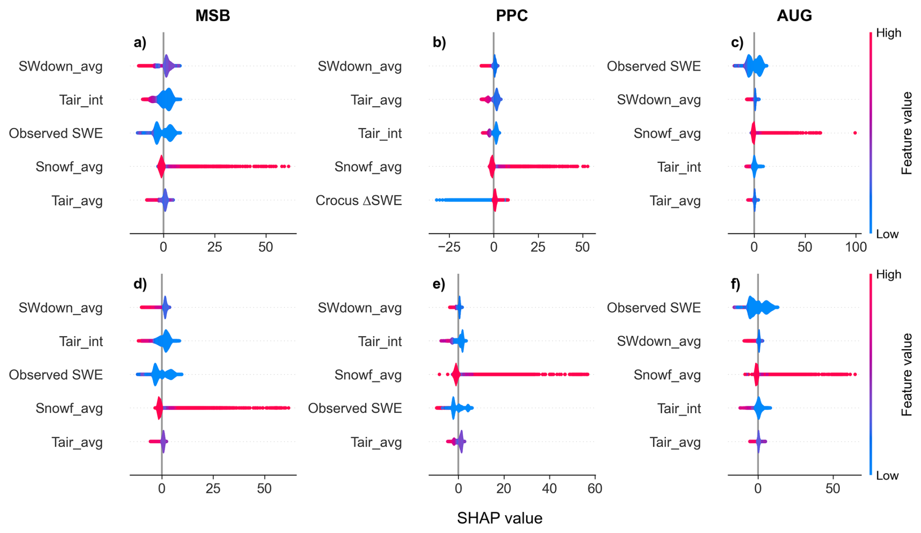
Figure C1 Violin plot of the SHAP values for the five most important variables (defined in Table 1) for the temporal (a–c) and station (d–f) splits and for each modelling setup. The colour indicates the normalized value of the feature.

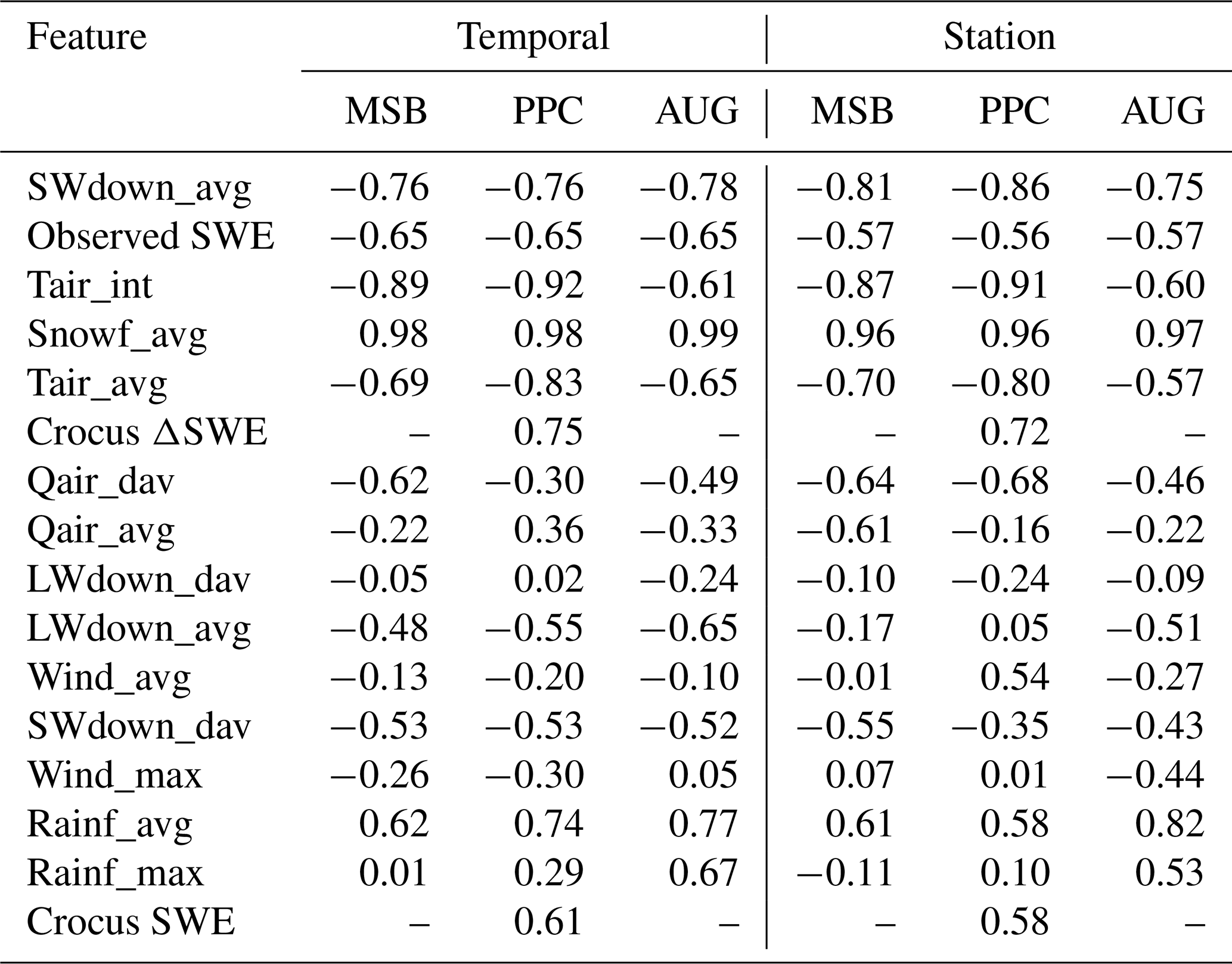
Another interesting aspect of feature importance is whether the features have generally a positive or negative influence in the predicted change in SWE. To assess that, the correlation between the variable and associated SHAP values is shown in Table C1. As expected, features related with air temperature and shortwave radiation have a strong negative correlation with the model-predicted ΔSWE, while the contrary is true for snowfall or the Crocus-simulated target.

Table C1 Correlation coefficient computed between each specific variable values and their associated SHAP value, for each data split and modelling setup.